Reflectance Properties of Hemiboreal Mixed Forest Canopies with Focus on Red Edge and Near Infrared Spectral Regions

Abstract

This study present the results of airborne top-of-canopy measurements of reflectance spectra in the spectral domain of 350–1050 nm over the hemiboreal mixed forest. We investigated spectral transformations that were originally designed for utilization at very different spectral resolutions. We found that the estimates of red edge inflection point by two methods—the linear four-point interpolation approach (S2REP) and searching the maximum of the first derivative spectrum ($D_{max}$) according to the mathematical definition of red edge inflection point—were well related to each other but S2REP produced a continuously shifting location of red edge inflection point while $D_{max}$ resulted in a discrete variable with peak jumps between fixed locations around 717 nm and 727 nm for forest canopy (the third maximum at 700 nm appeared only in clearcut areas). We found that, with medium high spectral resolution (bandwidth 10 nm, spectral step 3.3 nm), the in-filling of the O${}_2$-A Fraunhofer line ($F_{area}$) was very strongly related to single band reflectance factor in NIR spectral region ($\rho$ = 0.91, p < 0.001) and not related to Photochemical Reflectance Index (PRI). Stemwood volume, basal area and tree height of dominant layer were negatively correlated with reflectance factors at both visible and NIR spectral region due to the increase in roughness of canopy surface and the amount of shade. Forest age was best related to single band reflectance at NIR region ($\rho$ = −0.48, p < 0.001) and the best predictor for allometric LAI was the single band reflectance at red spectral region ($\rho$ = −0.52, p < 0.001) outperforming all studied vegetation indices. It suggests that Sentinel-2 MSI bands with higher spatial resolution (10 m pixel size) could be more beneficial than increased spectral resolution for monitoring forest LAI and age. The new index R${}_{751}$/R${}_{736}$ originally developed for leaf chlorophyll content estimation, also performed well at the canopy level and was mainly influenced by the location of red edge inflection point ($\rho$ = 0.99, p < 0.001) providing similar info in a simpler mathematical form and using a narrow spectral region very close to the O${}_2$-A Fraunhofer line.

1. Introduction

A strong interest is currently growing towards more extensive use of the red-edge and near infrared (NIR) spectral regions in vegetation remote sensing. New spaceborne sensors such as MultiSpectral Instrument (MSI) on board Sentinel-2 with special red-edge bands and Orbiting Carbon Observatory (OCO-2) for solar-induced chlorophyll fluorescence (SIF) retrievals based on in-filling of Fraunhofer lines in NIR spectral region have recently started to provide data with unprecedented quantity and quality [1]. Substantial research has been conducted during last decade to enable SIF retrievals from reflectance at global scale [2,3], and the future ESA FLEX mission (planned for launch by 2023) will improve the spatial resolution of space borne SIF estimates to about 300 × 300 m${}^2$.

The majority of ecophysiological research uses Pulse Amplitude Modulated (PAM) chlorophyll a fluorimetry to assess plant physiological state via chlorophyll fluorescence. Among PAM chlorophyll a fluorescence parameters the steady-state fluorescence yield at ambient light intensity has the best resemblance to SIF. Previous research has shown that at single leaf level up to 90% of variability for steady-state fluorescence yield can be explained by leaf growth irradiance, nitrogen content and plant species [4]. Absorbed light energy can be: (1) used for photosynthesis by photochemical energy conversion; (2) dissipated as heat; or (3) re-emitted as chlorophyll fluorescence. The first two processes are called photochemical and non-photochemical quenching, respectively, as both mechanisms reduce the chlorophyll fluorescence emission. If non-photochemical quenching (NPQ) is known or not changing, then chlorophyll fluorescence can be used to estimate photosynthesis. Active PAM chlorophyll a fluorimetry allows calculating parameters such as NPQ but not passive fluorescence measurement systems [5]. Xanthophyll cycle is the protective mechanism that regulates NPQ to dissipate excess energy safely as heat and it also causes a subtle change at leaf level absorption spectra [6]. Photochemical reflectance index (PRI) was originally constructed to assess the state of xanthophyll cycle via those spectral changes [7]. However, further research has revealed that PRI is also affected by numerous other factors such as pools of carotenoids and chlorophylls [8]. It has been shown that PRI at stand-level is not responding to the same physiological processes as at leaf level due to the effect of soil optical properties and canopy structure [9]. Factors such as blue sky radiation caused by scattering in the atmosphere and forest structure via within-canopy illumination variations and non-physiological shadowing effects affect PRI at canopy level in boreal forests [10,11]. In addition, variations in direct and diffuse surface irradiance have strong influence on the relationship between SIF and PRI [12]. To facilitate the future use of satellite derived SIF as an estimate of vegetation physiological state, leaf level studies on the relationships between PRI and different chlorophyll fluorescence parameters have been conducted [13,14].

Total chlorophyll fluorescence emission spectrum has two peaks at 685 nm (F685) and 740 nm (F740). It has been associated with the double-peak feature appearing in the red-edge spectral region of first derivative of vegetation reflectance and the ratio of the amplitude of the peaks by double-Gaussian fit has been used as an additional indicator of the photochemical activity of the plants [15].

Many different vegetation indices have been developed since the beginning of spaceborne vegetation remote sensing in the 1960s and 1970s. The main principle of traditional vegetation indices is to compare the reflectance in the visible spectral region where strong absorption by pigments is prevailing with reflectance in near infrared (NIR) plateau where wavelength-independent scattering dominates. Different wavelengths from visible (400–700 nm) to far-red/red-edge spectral region (700–730 nm) have been used to track pigment absorption features [16]. A review of different indices shows that in general vegetation indices that use only far-red spectral regions of longer wavelengths beyond 700 nm perform the best in predicting foliar chlorophyll content [17]. Pigment absorption declines sharply after 700 nm where the absorption maximum of the reaction center of photosystem I (P700) is located and this spectral region of fast change is called “red-edge”. This sharp increase in reflectance (decline in absorption) is the most characteristic feature of vegetation spectra and special methods including different spectral fitting [18] and linear extrapolation techniques for hyperspectral [19] and multispectral [20,21] data have been developed to track and determine the precise location of the fastest change. The signal in Sentinel-2 MSI bands 5 and 6 of 15 nm spectral resolution compared to each other and to the neighbor bands allows estimating the position and steepness of the red edge. The spatial resolution of these two narrow spectral bands is less than other visible and NIR bands (bands 2, 3, 4 and 8 of 10 m pixels) in order to guarantee the required signal-to-noise ratio.

Many remote sensing studies deal with crops and sparse vegetation where the change in the amount of biomass simultaneously changes the relative contribution of reflectance signal originating from soil. Soil background optical properties have crucial influence on reflectance signal measured above the vegetation in such sparse canopies and therefore soil adjustment would be needed to extract the information about vegetation characteristics [22]. The soil line concept has been used in formulation of many vegetation indices (e.g., Soil Adjusted Vegetation Index (SAVI) [23], Modified Chlorophyll Absorption Ratio Index Improved (MCARI2) [24], and Weighted (near-infrared-red) Difference Vegetation Index (WDVI) [25]). However, this approach would not be appropriate in the case of multi-layered closed forest canopies in our current study, where background signal would originate from lower layers of trees, herbaceous understory or moss-layer.

Remote sensing measurements can be made at various scales ranging from single leaf level observations in laboratory to top-of-atmosphere (TOA) satellite observations [26]. Airborne hyperspectral imagers CASI [27] and APEX [28] provide high quality spectral at-sensor radiance data. Such data or even non-calibrated digital numbers by new lightweight hyperspectral imagers [29] can provide vegetation indices or perform classification of targets. For top-of-canopy spectral reflectance, simultaneous measurements of irradiance spectra are needed and, in the case of high-flying airborne measurements [30], atmospheric correction is needed. Our study focused on the intermediate scale of so-called bottom-of-atmosphere (BOA)/top-of-canopy (TOC) measurements above mixed forest canopy. Low-level airborne spectral data are supported by simultaneous recording of irradiance spectra to convert airborne data to TOC spectral directional reflectance, and by forestry data provided by the National forestry database. The aim of the current study was to explore the inter-relationships between different spectral features of apparent top-of-canopy reflectance of hemiboreal mixed forest using measurements with medium or high spectral resolution, most commonly available for airborne spectral measurements and forest inventory variables.

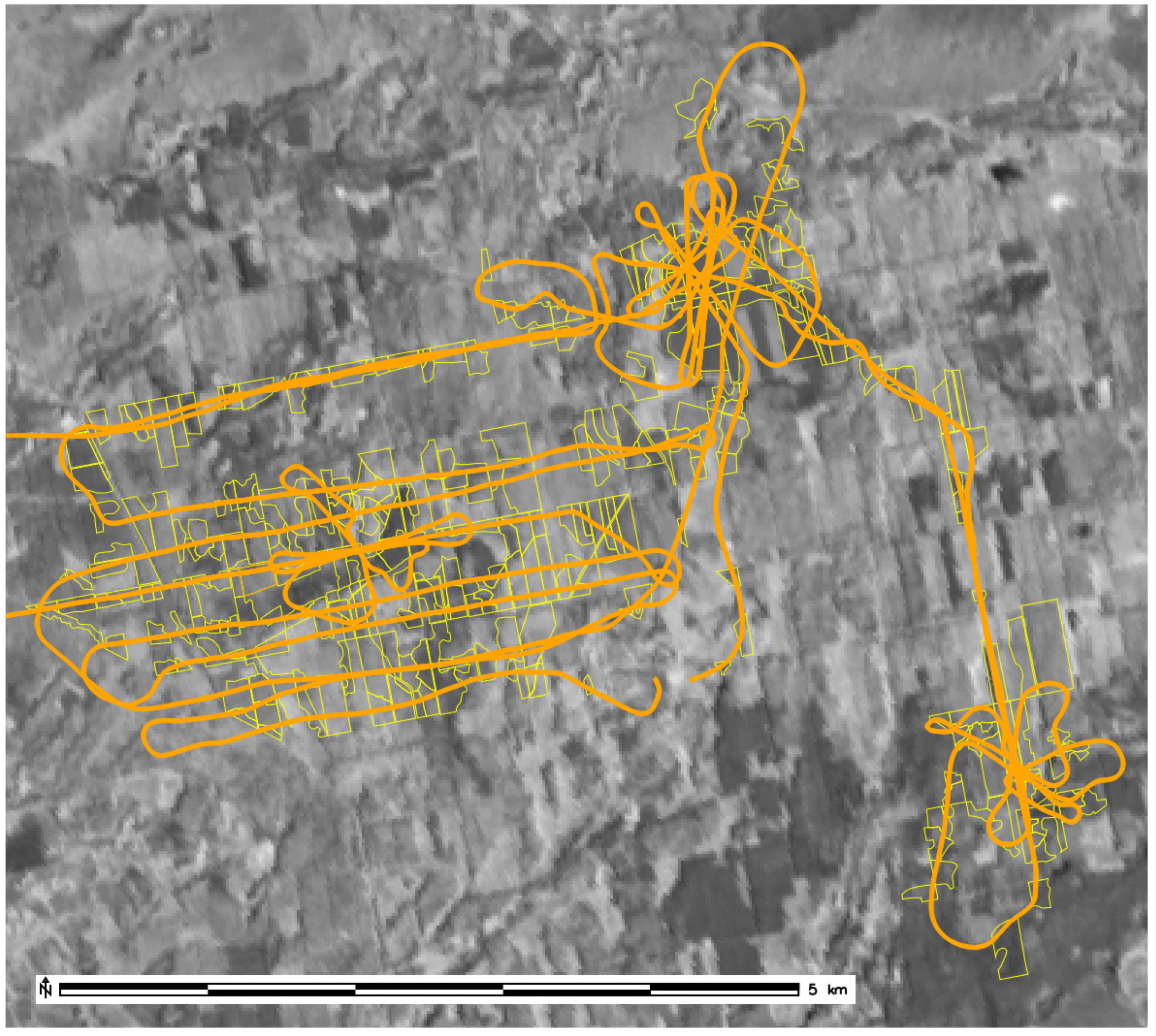
2. Material and Methods

Airborne measurements of VisNIR directional reflectance were carried out over hemiboreal forests at the Järvselja test site in southeastern Estonia in summer 2010. The coordinates of the test site are 58.3°N, 27.3°E. The landscape at the test site is plain, and the ground height is 30–40 m asl. There are mixed forests which belong to the hemiboreal zone with moderately cool and moist climate and can be characterized as remote and rural with low anthropogenic disturbances. Stands are pure or mixed and composed mainly of silver birch (Betula pendula), Scots pine (Pinus sylvestris), Norway spruce (Picea abies), common alder (Alnus glutinosa), aspen (Populus tremula), grey alder (Alnus incana), and small-leaved lime (Tilia cordata). A forest stand is a patch of homogeneous forest considering its species composition, age, tree height, tree density, and site type. A forest management inventory database including 1:10,000 map of stands is available for Järvselja Training and Experimental Forest district. The database is updated regularly. Several forest parameters such as species composition, age, breast-height diameter (cm), tree height H (m), basal area for the dominant and secondary layers G1 and G2 (m${}^2$/ha), stem volume for the dominant and secondary layer M1 and M2 (m${}^3$/ha), stem volume increment Z${}_v$ (m${}^3$/ha/year), site type, etc. have been recorded for every stand. The minimal area of a stand is 0.1 ha according to the requirements by national forest inventory. Growth conditions at the study site range from poor where the site index H${}_{100}$ (stand height at the stand age of 100 years) is less than 10 m to very good where H${}_{100}$ can be over 35 m. About 75% of the site area is forests, natural grasslands, and pastures. A more detailed description of the test site was provided by Kuusk et al. [31]. Clear-cut areas and stands younger than 15 years were removed from the current analyses. The final dataset reported here consists of 300 forest stands aged between 15 and 230 years. The stand areas are between 0.2 and 14.9 ha. The average stand age is 60 and median 54 years. Allometric estimate of tree layer leaf area index (LAI) ranged from 1 to 9 (mean and median 4.5).

Helicopter measurements of reflectance spectra in the spectral domain 350–1050 nm over the study area were carried out using UAVSpec3 spectrometer on 5 July 2010 (Figure 1). The spectrometer UAVSpec3 is a fully autonomous lightweight spectrometer based on the 256-band near-infrared (NIR) enhanced version of the miniature spectrometer module Monolithic Miniature Spectrometer 1 (MMS-1) manufactured by Carl Zeiss Jena GmbH [32]. The spectral resolution of the spectrometer is 10 nm and the spectral sampling interval is 3.3 nm. The spectrometer was mounted on the chassis of a Robinson R22 helicopter so that it was looking in the nadir direction during straight flight at constant speed. Average flight altitude was about 80–100 m above ground level and the flight speed was 60 km/h. The footprint of the field-of-view (FOV) of the spectrometer on the ground was about 2.5–3 m, and spectra were recorded at the frequency eight spectra per second. Measurements were carried out in direct sunlight at solar zenith angle (SZA) of approximately 40°. For the measurements of incident spectral radiation, the HR-1024 spectrometer by Spectra Vista Corporation equipped with a cosine receptor RCR/A124505 by Analytical Spectral Devices, Inc. was used. The SVC HR-1024 spectrometer has a spectral range of 350–2500 nm, 1024 spectral bands, and a bandwidth of about 1.5 nm in the wavelength range 350–1000 nm. Incoming spectral flux was measured at a nearby clearing.

Raw data from the airborne spectral sensor were corrected for dark signal temperature dependence and spectral stray light. The method suggested by Kuusk [33] was used for dark signal correction. Stray light was corrected with the deconvolution method proposed by Kostkowski [34] for spectral instruments. Instrument function of the spectral sensor was characterized using a double monochromator, as described by Kuusk et al. [35]. The recorded digital numbers were converted to directional reflectance factor using simultaneous measurements of incoming spectral flux, calibration coefficients of every sensor element determined by measuring the calibrated grey reference panel SRT-20-120 by Labsphere Inc. [36], and correcting recorded signals for dark current and stray light in the spectral sensor (Figure 2),

$$R_{\lambda }\left(t\right)=\frac{q_{\lambda }\left(t_0\right)}{n_{\lambda }\left(t_0\right)}\frac{n_{\lambda }\left(t\right)}{q_{\lambda }\left(t\right)}{r}_{\lambda }.$$

(1)

Here, $R_{\lambda }\left(t\right)$ is the spectral directional reflectance of the target at nadir (${\theta }_v=0$°) at wavelength $\lambda$ measured at time moment t; $q_{\lambda }\left(t\right)$ and $q_{\lambda }\left(t_0\right)$ are the signals of incoming flux during the target measurements and calibration, respectively; $n_{\lambda }\left(t\right)$ and $n_{\lambda }\left(t_0\right)$ are the signals of the UAVSpec sensor element which corresponds to the wavelength $\lambda$; and $r_{\lambda }$ is the spectral reflectance factor of the reference panel. All the signals in Equation (1) were corrected for dark current and the sensor signals $n_{\lambda }\left(t\right)$ were corrected for stray light. The spectral resolution of the MMS-1 is less than that of the HR-1024; therefore, the recorded spectra of HR-1024 were filtered to the spectral resolution of UAVSpec3 using respective band-pass filter, and resampled to the wavelengths of UAVSpec3 before applying Equation (1). As the distance between the top of forest stands and sensor was only 50–80 m, no atmospheric correction was applied. Measurements were carried out in stable illumination conditions. The calibration errors of spectrometers were reduced by using ratio of spectrometer signal in Equation (1). The uncertainty of the reference $r_{\lambda }$ by Labsphere Inc. is less than 0.005 for the spectral range 300–2200 nm. In the following analysis included the stands over which at least 10 spectra were recorded. Spectra were sampled with the spatial step of 2.1 m on the flight transect. The footprint of the field-of-view of the UAVSpec at the flight height of 80 m is a circle of the diameter of 3 m. The range of the number of recorded spectra over a stand varied in general from 10 to 130, except for three mature stands over which several passes were done and the number of recorded spectra reaches 1300. Recorded spectra in the buffer zone of 8 m at the stand borders were not considered.

Average spectrum of the directional reflectance factor for every stand was calculated (Figure 3A). The term Vegetation Index (VI) refers to a spectral transformation of two or more discrete spectral bands to enhance their sensitivity to vegetation properties. The most commonly used formulation of VI is the Normalized Difference Vegetation Index (NDVI).

$$NDVI[{\lambda }_1;{\lambda }_2]=\frac{(R_{\lambda 2}-R_{\lambda 1})}{(R_{\lambda 2}+R_{\lambda 1})}.$$

(2)

It can be calculated for any spectral bands. The simplest form of VI is:

$$\frac{R_{\lambda 2}}{R_{\lambda 1}},$$

(3)

called Simple Ratio (SR).

Using spectral bands at 736 nm and 751 nm wavelengths suggested by Hallik et al. [17], we found that SR (Equation (4)) and NDVI (Equation (5)) forms were almost linearly related to each other (Figure 4C) and therefore we used only a single formulation of Equation (4) in this study.

$$R_{751}/R_{736}=\frac{R_{751}}{R_{736}},$$

(4)

$$NDVI[751;736]=\frac{(R_{751}-R_{736})}{(R_{751}+R_{736})}.$$

(5)

The other four vegetation indices used in this study ($PRI$ [7], $NDV{I}_{665}$ [37], $NDV{I}_{705}$ [38], and $S2REP$ [20,21]) were calculated as:

$$PRI=\frac{(R_{531}-R_{570})}{(R_{531}+R_{570})},$$

(6)

$$NDV{I}_{665}=\frac{(R_{783}-R_{665})}{(R_{783}+R_{665})},$$

(7)

$$NDV{I}_{705}=\frac{(R_{783}-R_{705})}{(R_{783}+R_{705})},$$

(8)

$$S2REP=705+35\left(\frac{{\displaystyle \left(\frac{R_{783}+R_{665}}{2}\right)-R_{705}}}{R_{740}-R_{705}}\right).$$

(9)

S2REP is the equation for the linear four-point interpolation approach based on the work of Guyot and Baret [20] and Clevers et al. [21] to calculate the red-edge inflection point using Sentinel-2 MSI spectral bands. The first derivative of reflectance spectra was calculated to find the true location of maximal change for each stand (Figure 3B).

For the estimation of the sun-induced fluorescence, the spectral signatures of stands in the wavelength interval 752–765 nm were analyzed (Figure 3C). At 761 nm, the incident sun radiation is strongly absorbed by oxygen absorption band O${}_2$-A in the atmosphere. In the recorded UAVSpec3 signal, the weak signal of reflected radiation is overlapped by the emitted radiation of sun-induced fluorescence [39], therefore Equation (1) returns the biased result

$$R\left(\lambda \right)=\frac{(b_r\left(\lambda \right)+b_f\left(\lambda \right))}{b_e\left(\lambda \right)},$$

(10)

where $b_r\left(\lambda \right)$ is the reflected radiance, $b_f\left(\lambda \right)$ is the radiance of fluorescence, and $b_e\left(\lambda \right)$ is the radiance of a non-absorbing Lambertian surface of no fluorescence at similar illumination conditions.

Contact laboratory measurements of reflectance spectra of landscape components—green leaves, tree stems and branches, and soil—using light source of no absorption lines show that all these spectra are smooth in the wavelength range 722–791 nm [40]. Thus, in the case of no fluorescence, the apparent reflectance of forests were smooth too. This smooth spectrum is found by smoothing the recorded spectra in the wavelength range 722–791 nm by spline-approximation, omitting recorded values at 752–765 nm. This smoothed spectrum is called “continuum”. The difference of the recorded apparent reflectance and continuum near the absorption line at 761 nm is caused by the sun-induced fluorescence. The spectral resolution of UAVSpec3 is too low for recording the exact profile of the forest signal near 761 nm. The peak of apparent reflectance factor is spread by instrumental averaging over the spectral band 752–765 nm determined by the spectral sensitivity profile of the MMS-1. Therefore, the quantitative measure of the fluorescence contribution in the apparent reflectance is the area (not height) of the peak above the continuum near the absorption line at 761 nm,

$$F_{area}={\int }_{\Delta \lambda }(R\left(\lambda \right)-R_c\left(\lambda \right))d\lambda ,$$

(11)

where $\Delta \lambda$ is the wavelength interval 751.7–768.2 nm and $R_c\left(\lambda \right)$ is the smoothed spectrum (continuum) (see Figure 3C).

All statistical tests were performed with R version 3.4.4 (2018-03-15) [41]. Spearman rank order correlation was used to assess the strength and direction of association between variables because some pairwise relationships were nonlinear. The significance level of 0.05 was used.

3. Results

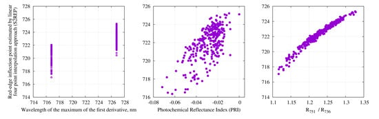
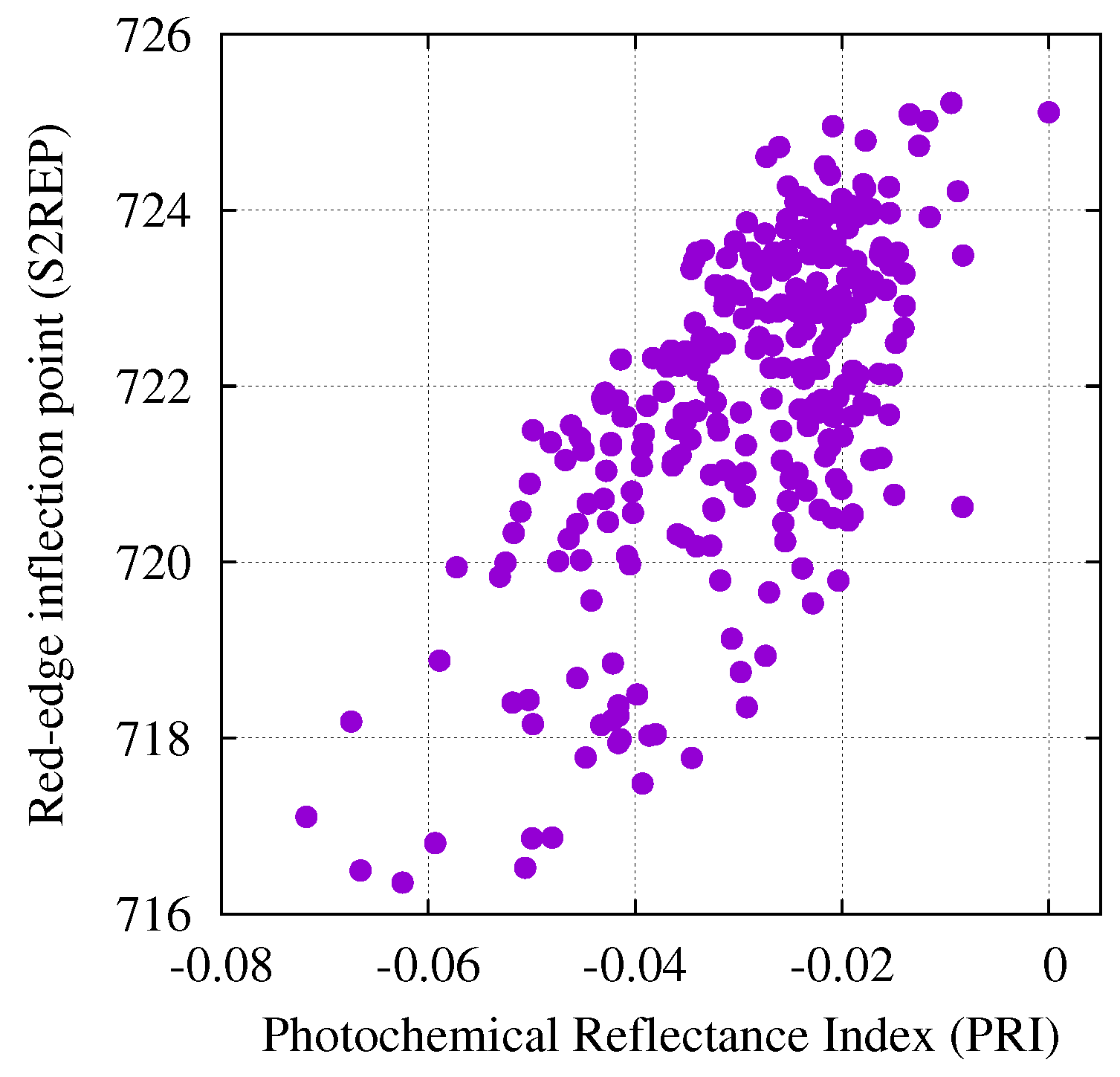
3.1. Comparison of Different Methods to Calculate Red-Edge Inflection Point

Sentinel-2 MSI has special spectral bands located in red-edge spectral region to calculate the red-edge inflection point using the linear four-point interpolation approach. We used the same method to calculate the parameter we call Red-Edge inflection Point Vegetation Index (S2REP) from top-of-canopy high resolution reflectance spectra measured from helicopter. To estimate the true red-edge inflection point, we calculated the first derivative of reflectance spectrum and searched the location of the maximum of the first derivative in red-edge spectral region. We found that the derivative spectrum had two local maximums at constant wavelengths and the shift of the location of red-edge inflection point was determined solely by which one of the two local maximums was higher (Figure 3B and Figure 5). Initially, we found three distinct possible locations at 700 nm, 717 nm and 727 nm (Figure 3B) for the maximum of the first derivative but the first location of maximum at 700 nm disappeared when we removed clearcut patches from further analysis (data not shown). Only two discrete wavelengths at 717 nm and 727 nm came out as the true locations of the maximum of the first derivative across all forest spectra in our dataset. Among 300 forest stands, the maximum of the first derivative was found to be either at 717 nm or 727 nm and no other wavelengths came out as the location of red-edge inflection point. There was still a very strong relationship between the red-edge inflection point estimates with both methods (Figure 5). For the sake of mathematical simplicity we used the S2REP index in Equation (9) as the estimate of red-edge inflection point in further statistical tests since it turned out to be a continuous parameter while the true location of the maximum of the first derivative in red-edge spectral region appeared to be a discrete parameter (Figure 5).

3.2. Correlation Between Single Band Reflectance Factors and Spectral Transformations

There was a very strong positive correlation between the in-filling of the O${}_2$-A Fraunhofer line ($F_{area}$) and single band reflectance factors at NIR plateau (the coefficient of Spearman’s rank-order correlation $\rho$ = 0.91, p < 0.001). The relationship was absent in spectral regions close to absorption maxima (blue and red) and increased with increasing reflectance (

Table 1. Spearman’s rank-order correlation coefficients between single band reflectance factors in blue (490 nm), green (531 nm and 570 nm), red (665 nm), red-edge (705 nm) and near infrared (736 nm, 740 nm, 751 nm and 783 nm) spectral regions and spectral transformations: in-filling of the O${}_2$-A Fraunhofer line around 760 nm ($F_{area}$), Photochemical Reflectance Index (PRI), red NDVI (NDVI${}_{665}$), red-edge NDVI (NDVI${}_{705}$), new simple ratio at 736 nm and 751 nm (R${}_{751}$/R${}_{736}$), and red-edge inflection point estimated by linear four-point interpolation approach (S2REP). Asterisks denote statistical significance.

	${\mathit{F}}_{\mathit{a}\mathit{r}\mathit{e}\mathit{a}}$	PRI	NDVI${}_{665}$	NDVI${}_{705}$	R${}_{751}$/R${}_{736}$	S2REP
R${}_{490}$	0.10 ns	−0.48 ***	−0.34 ***	−0.43 ***	−0.49 ***	−0.47 ***
R${}_{531}$	0.35 ***	−0.47 ***	−0.08 ns	−0.27 ***	−0.35 ***	−0.37 ***
R${}_{570}$	0.32 ***	−0.56 ***	−0.12 *	−0.31 ***	−0.41 ***	−0.42 ***
R${}_{665}$	−0.06 ns	−0.62 ***	−0.53 ***	−0.60 ***	−0.65 ***	−0.63 ***
R${}_{705}$	0.51 ***	−0.59 ***	0.10 ns	−0.10 ns	−0.25 ***	−0.25 ***
R${}_{736}$	0.88 ***	−0.14 *	0.69 ***	0.55 ***	0.39 ***	0.40 ***
R${}_{740}$	0.89 ***	−0.09 ns	0.73 ***	0.59 ***	0.44 ***	0.45 ***
R${}_{751}$	0.91 ***	−0.03 ns	0.77 ***	0.65 ***	0.51 ***	0.52 ***
R${}_{783}$	0.91 ***	−0.01 ns	0.79 ***	0.67 ***	0.53 ***	0.54 ***

*** p < 0.001; * p < 0.05; ns p > 0.05. Bold font indicates the spectral bands for calculating given vegetation index.

). The correlations between $F_{area}$ and single band reflectance factors were moderately strong in green spectral region and the strongest at NIR plateau. The relationship between PRI and single band reflectance factors was stronger in visible and red-edge spectral region while it disappeared at NIR plateau (Table 1).

The normalized difference vegetation index NDVI was calculated using two different “sensitive” wavelengths: one in the red spectral region close to the chlorophyll absorption maximum at 665 nm (NDVI${}_{665}$) and the other in the red-edge at 705 nm (NDVI${}_{705}$). The same “reference” wavelength was used in both cases at 783 nm. In general, both indices had negative correlation with single band reflectance factors at visible spectral domain and positive with reflectance at NIR plateau. It is noteworthy that NDVI${}_{665}$ had almost no relationship with reflectance at red-edge spectral region and weaker correlation with green reflectance, which are generally considered more informative spectral regions. NDVI${}_{705}$ had generally stronger correlations than NDVI${}_{665}$ with reflectance factors at visible spectral region. Opposite to what could be expected, NDVI${}_{705}$ had the weakest correlation with the reflectance factor at 705 nm despite of the fact that it was actually used to calculate NDVI${}_{705}$. At the same time, the single band reflectance factor at 665 nm was also slightly more correlated to NDVI${}_{705}$ than to NDVI${}_{665}$. The general tendency that vegetation indices (except NDVI${}_{665}$) had stronger correlation with single band reflectance factors at some other wavelengths and not at those bands which were used for calculating the index itself, was particularly clear in our new vegetation index R${}_{751}$/R${}_{736}$ (Table 1), indicating that such spectral transformations give some additional information about vegetation not provided by simple reflectance factors. S2REP and R${}_{751}$/R${}_{736}$ both had very similar relationships with single band reflectance factors. All four vegetation indices that should be sensitive to the amount of green biomass (NDVI${}_{665}$, NDVI${}_{705}$, R${}_{751}$/R${}_{736}$ and S2REP) had stronger correlation with single band reflectance factor at red spectral region close to chlorophyll absorption maximum than at green or red-edge regions.

3.3. Relationships Between Spectral Transformations

Table 2. Relationships between spectral transformations: in-filling of the O${}_2$-A Fraunhofer line around 760 nm ($F_{area}$), Photochemical Reflectance Index (PRI), red NDVI (NDVI${}_{665}$), red-edge NDVI (NDVI${}_{705}$), new simple ratio at 736 nm and 751 nm (R${}_{751}$/R${}_{736}$), and red-edge inflection point estimated by linear four-point interpolation approach (S2REP). Asterisks denote statistical significance of Spearman’s rank-order correlation coefficients.

	${\mathit{F}}_{\mathit{a}\mathit{r}\mathit{e}\mathit{a}}$	PRI	NDVI${}_{665}$	NDVI${}_{705}$	R${}_{751}$/R${}_{736}$	S2REP
$F_{area}$	1
PRI	−0.05 ns	1
NDVI${}_{665}$	0.76 ***	0.36 ***	1
NDVI${}_{705}$	0.66 ***	0.50 ***	0.94 ***	1
R${}_{751}$/R${}_{736}$	0.53 ***	0.64 ***	0.85 ***	0.95 ***	1
S2REP	0.54 ***	0.60 ***	0.85 ***	0.97 ***	0.99 ***	1

*** p < 0.001; ns p > 0.05.

summarizes the correlations between the main spectral transformation parameters under focus of the current study. These inter-correlations must be considered when interpreting the relationships between forest parameters and spectral characteristics.

In a leaf level study [17], we found that the simple ratio of reflectances at 751 nm and 736 nm was the best predictor of leaf chlorophyll content. To assess how such long wavelengths would operate at canopy level, we calculated the same index in our current study. We compared it with other indices, as illustrated in Figure 4. The simple ratio of reflectances at 751 nm and 736 nm responds at canopy level similarly to more conventional red edge indices, as shown in Figure 4A,B, suggesting that vegetation index R${}_{751}$/R${}_{736}$ can be used both at leaf level and at canopy level. Usually, vegetation indices that utilize the same reflectance bands but formulated as normalized difference (NDVI) and simple ratio (SR) are nonlinearly related to each other [17]. Figure 4C shows that, if the vegetation index is constructed using reflectance at 751 nm and 736 nm, then in our dataset NDVI and SR forms are almost linearly related to each other. Hence, we use only the simpler form (SR) of this vegetation index.

There was a remarkably strong correlation between red-edge inflection point (S2REP) and other vegetation indices, particularly R${}_{751}$/R${}_{736}$ ($\rho$ = 0.99, Figure 4A) and NDVI${}_{705}$ ($\rho$ = 0.97) but also NDVI${}_{665}$ ($\rho$ = 0.85) and PRI ($\rho$ = 0.60; Figure 6).

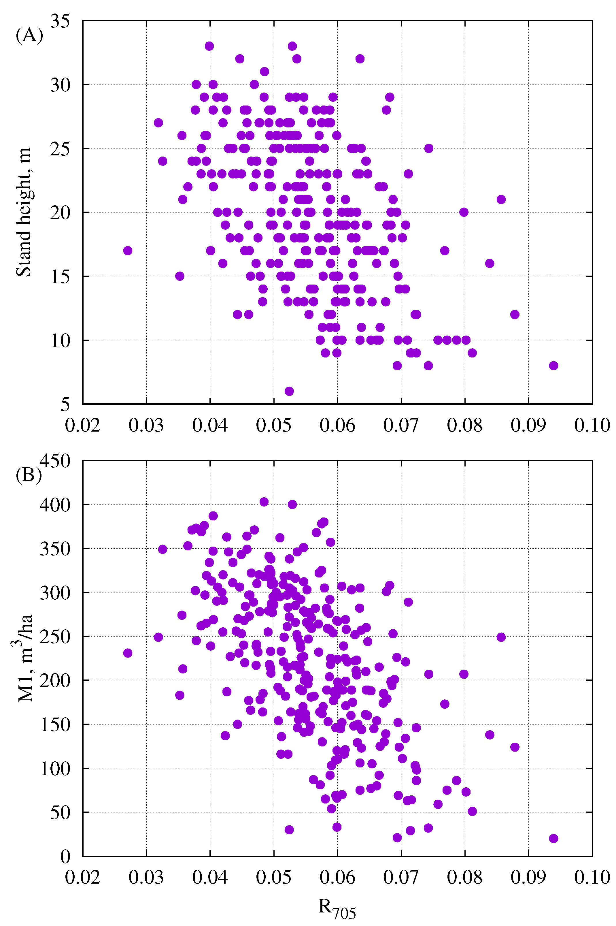
3.4. Relationships Between Reflectance and Some Parameters from Forest Inventory Data

We selected seven variables from forest inventory data (

Table 3. Spearman’s rank-order correlation coefficients among forest inventory variables (site index (H${}_{100}$), stem volume increment (Z${}_v$), basal area for dominant layer (G1), stemwood volume for dominant layer (M1), height of the tree with average basal area also known as Lorey’s height (H), allometric estimate of leaf area index (LAI) and stand age), single band reflectance factors in visible and near infrared spectral regions and spectral transformations (in-filling of the O${}_2$-A Fraunhofer line around 760 nm ($F_{area}$), Photochemical Reflectance Index (PRI), Normalized Difference Vegetation Indices (NDVIs), new simple ratio at 736 nm and 751 nm (R${}_{751}$/R${}_{736}$), and red-edge inflection point estimated by linear four-point interpolation approach (S2REP)). Asterisks denote statistical significance.

	H${}_{100}$ (m)	Z${}_{\mathit{v}}$ (m${}^3$/ha/year)	G1 (m${}^2$/ha)	M1 (m${}^3$/ha)	H (m)	LAI	Age (yr)
R${}_{490}$	−0.37 ***	−0.31 ***	−0.16 **	−0.23 ***	−0.20 ***	−0.50 ***	0.11 ns
R${}_{531}$	−0.35 ***	−0.14 *	−0.38 ***	−0.48 ***	−0.45 ***	−0.39 ***	−0.17 **
R${}_{570}$	−0.40 ***	−0.17 **	−0.40 ***	−0.50 ***	−0.46 ***	−0.41 ***	−0.15 **
R${}_{665}$	−0.41 ***	−0.33 ***	−0.14 *	−0.19 ***	−0.17 **	−0.52 ***	0.17 **
R${}_{705}$	−0.36 ***	−0.14 *	−0.50 ***	−0.57 ***	−0.47 ***	−0.33 ***	−0.25 ***
R${}_{736}$	0.02 ns	0.12 *	−0.45 ***	−0.44 ***	−0.30 ***	−0.005 ns	−0.47 ***
R${}_{740}$	0.05 ns	0.13 *	−0.43 ***	−0.42 ***	−0.28 ***	0.02 ns	−0.47 ***
R${}_{751}$	0.10 ns	0.16 **	−0.40 ***	−0.39 ***	−0.25 ***	0.05 ns	−0.48 ***
R${}_{783}$	0.11 ns	0.17 **	−0.39 ***	−0.38 ***	−0.24 ***	0.06 ns	−0.48 ***
$F_{area}$	0.18 **	0.24 ***	−0.29 ***	−0.30 ***	−0.20 ***	0.15 **	−0.46 ***
PRI	0.56 ***	0.33 ***	0.34 ***	0.37 ***	0.30 ***	0.30 ***	−0.05 ns
NDVI${}_{665}$	0.31 ***	0.30 ***	−0.19 ***	−0.18 **	−0.09 ns	0.32 ***	−0.46 ***
NDVI${}_{705}$	0.43 ***	0.30 ***	−0.06 ns	0.01 ns	0.10 ns	0.38 ***	−0.35 ***
R${}_{751}$/R${}_{736}$	0.52 ***	0.37 ***	0.01 ns	0.07 ns	0.12 *	0.42 ***	−0.34 ***
S2REP	0.49 ***	0.33 ***	0.02 ns	0.09 ns	0.15 **	0.39 ***	−0.31 ***

* p < 0.05; ** p < 0.01; *** p < 0.001; ns p > 0.05.

). In most of our studied forestry parameters, negative relationships with reflectance in both NIR and visible spectral regions were generally prevailing and the best predictors tended to be single band reflectance factors not vegetation indices. The two exceptions were stem volume increment (Z${}_v$), which had the strongest correlation with our new vegetation index R${}_{751}$/R${}_{736}$, and H${}_{100}$ (expected stand height at the stand age of 100 years), which had the strongest relationship with PRI (Table 3). Three parameters related to tree trunk size—G1, M1 and Lorey’s height (H)—had the strongest correlation with single band reflectance factor at red-edge spectral region R${}_{705}$ (Figure 7) and LAI with red spectral regions. The best predictor for forest age was reflectance at NIR plateau (Table 3).

LAI was slightly better correlated with R${}_{751}$/R${}_{736}$ than with NDVI${}_{665}$ or NDVI${}_{705}$ but the best predictor for LAI was single band reflectance in red spectral region ($\rho$ = −0.52, p < 0.001). PRI had positive correlations with H${}_{100}$, Z${}_v$, G1, M1, H and LAI (Table 3).

4. Discussion

4.1. Comparison of Different Methods to Calculate Red-Edge Inflection Point

The abrupt increase of reflectance from red to NIR spectral region is the most notable and characteristic feature of vegetation spectra. This region of rapid change is called “red edge”. To provide quantitative measure for this spectral feature, the location of the fastest change has been defined as “red edge inflection point”. By the mathematical definition red edge inflection point is the location of the maximum of the first derivative of reflectance within the red edge spectral region. High resolution reflectance spectrum is required to calculate the first derivative spectrum. Such information is available from leaf level, ground level and TOC airborne spectral measurements. Current spaceborne sensors do not measure high resolution full spectra and therefore require different methodology. For multi-spectral data with limited number of distinct spectral bands, the linear four-point interpolation approach has been proposed. This method is essentially a vegetation index using four spectral bands to estimate red edge inflection point. For example, Sentinel-2 MSI has a number of spectral bands located in the red-edge spectral region to calculate the red-edge inflection point using the linear four-point interpolation approach based on the work of Guyot and Baret [20] and Clevers et al. [21]. As we used the formula suggested for Sentinel-2 bands, we also used the name S2REP for this vegetation index. Shifts in red edge inflection point location have been traditionally associated with leaf chlorophyll content and green biomass (e.g., [42]). When we calculated the actual red edge inflection point location from the first derivatives spectrum, we did not observe any gradual shifts but only two discrete locations appeared around 717 nm and 727 nm. UAVSpec3 has 3.3 nm sampling interval, thus there are two spectral measurements/bands between 717 nm and 727 nm and the two-modal result cannot be explained only by the low spectral sampling interval of the spectrometer. A somewhat similar effect of peak jump has also been demonstrated at leaf level [18]. At canopy level, the number of distinct peaks locations appeared to depend on growth form as the third location of first derivatives maximum occurred at 700 nm and disappeared after the removal of clearcut plots. The double-peak feature associated previously with photochemical activity of the plants by Alonso et al. [15] would correspond to the peak at 700 nm and can ot explain the jumps between two other peaks at 717 nm and 727 nm. For example, Kochubey and Kazantsev [43] found at leaf level measurements of agricultural crop also three peaks at similar wavelength as we observed at canopy level over forests. Contradicting opinions exist about the possible mechanism of peak jumps, as it has been explained either simply as the effect of the amount of chlorophyll [44] or as the result of photochemical activity and chlorophyll flourescence [15]. We can show that the phenomenon exists but laboratory analysis of fine-scale absorption features of different pigment–protein complexes would be needed to provide explanation.

Comparison of two methods reveals that, when we estimated red edge inflection point location by searching the maximum of the first derivative in red edge region, it resulted in a clearly discrete parameter but the result of linear four-point interpolation approach (S2REP) was a continuous parameter displaying a gradual shift in the estimated location of red edge inflection point. This will clearly require further studies to clarify the mechanism behind the “peak-jump” observed in red edge inflection point estimated from high resolution spectra. Nevertheless, both methods were in good agreement and both estimates were strongly related to each other (Figure 5), thus we used only S2REP index in statistical tests to represent the single location of red edge inflection point (Table 1, Table 2 and Table 3). Alternative linear extrapolation techniques exist [19].

4.2. The In-Filling of the O${}_2$-A Fraunhofer Line

To estimate accurately sun-induced chlorophyll fluorescence (SIF) from the in-filling of the O${}_2$-A Fraunhofer line around 760 nm, a sub-nanometer spectral resolution would be advised [45,46], nonetheless there have been previous studies using much lower spectral resolution for airborne hyperspectral measurements while interpreting the measured in-filling of the O${}_2$-A Fraunhofer line as estimate of chlorophyll fluorescence emission (e.g., [47,48]). We cannot record the exact profile of the forest signal near 760 nm due to the low spectral resolution of the used spectrometer [32]. The apparent reflectance factor corresponds to the instrumental averaging over the spectral band determined by the spectral sensitivity profile of MMS-1 and traditional Fraunhofer line discrimination methods [39] would give biased results. Therefore, we used the area of the peak as shown in Equation (11) instead of the height for the quantitative measure of the in-filling of the O${}_2$-A Fraunhofer line $F_{area}$ in our data. To avoid speculations, we call the variable which we measured strictly as the in-filling of the O${}_2$-A Fraunhofer line and not chlorophyll fluorescence, although the measured signal must also contain significant contribution of SIF [49,50].

When the in-filling of the O${}_2$-A Fraunhofer line ($F_{area}$) was measured as the area of apparent peak in our current studies with medium spectral resolution above mixed forest canopy, the value of $F_{area}$ mainly corresponded to forest brightness in NIR spectral region (Table 1) and $F_{area}$ was related to vegetation indices and forestry parameters, which had strong correlation with single band reflectance factors at NIR plateau.

Among the studied vegetation indices, PRI should be mechanistically the most closely related to chlorophyll fluorescence via response to non-photochemical quenching of fluorescence [7]. Nevertheless, PRI was the only vegetation index not correlated to $F_{area}$ at all in our study since PRI was also the only vegetation index not correlated with reflectance at NIR spectral region (Table 1). PRI is not responding to the same physiological processes at stand level as at leaf level because of PRI at stand level is affected by a range of non-physiological factors such as background optical properties and canopy structure [9]. It has been shown in boreal forests that factors such as forest structure via within-canopy illumination variations and non-physiological shadowing effects affect PRI at canopy level as well as blue sky radiation caused by scattering in the atmosphere [10,11]. Therefore, we cannot distinguish whether the decoupling between PRI and $F_{area}$ is due to the structural or physiological control mechanisms. However, we can confirm the existence of this phenomenon (decoupling of PRI) at forest canopy bottom-of atmosphere (BOA) reflectance data and it can be relevant ground information for future satellite missions such as FLEX, which will measure top-of-atmosphere (TOA) PRI and SIF.

NDVI${}_{665}$, which was the most strongly correlated with NIR reflectance, also had the strongest correlation with $F_{area}$ (Table 2). The relationship between $F_{area}$ and S2REP used as a proxy of red-edge inflection point was moderately strong ($\rho$ = 0.54, p < 0.001) and in similar magnitude as correlation between S2REP and single band reflectance factors at NIR region (Table 1). All empirical correlations with $F_{area}$ appeared to be dominated by the effect of forest brightness at NIR plateau in our study. SIF is driven by solar irradiance and mechanistically related to the total absorbed PAR as well as vegetation stress [46]. The strong association between $F_{area}$ and NIR reflectance could be interpreted from the view point of canopy shadow fraction as the effect of sunlit fraction of foliage should be manifested more clearly in NIR reflectance.

4.3. The Relationships Between Vegetation Indices, Single Band Reflectance Factors and Forestry Parameters

In agricultural crops or sparse vegetation, the reflectance in NIR region increases as the amount of biomass increases above soil. The forest ecosystem is an environment of shade. In hemiboreal forests, the canopy brightness in NIR starts to decrease due to the increase in the roughness of the forest canopy as a surface as forest grows higher and biomass increases [51]. The amount of shade will increase with stand age. At the early age before canopy closure, the proportion of sunlit ground vegetation decreases as trees grow bigger. After the maximum canopy closure is attained, LAI will not change much but stemwood volume and tree height can continue growing [51,52].

Our current study showed that the best predictor for forest age was reflectance in NIR region. Younger forest stands appeared to be brighter in NIR spectral region. A similar effect was shown by Rautiainen et al. [53] when comparing spectral properties of mature and immature forest stands and by Nilson and Peterson [51] studying successional reflectance trajectories of birch, pine and spruce dominated stands. Changes in canopy closure, LAI, species composition and background reflectance have been shown to control the relationship between stand age and reflectance [51].

We calculated two NDVIs with different wavelengths. NDVI${}_{665}$ using red spectral region where the reflectance signal should saturate more quickly with increased green biomass and NDVI${}_{705}$ calculated from wavelengths with less absorption to avoid saturation. When we compared the NDVI values with single band reflectance factors at different wavelengths, it appears that NDVI${}_{705}$ had stronger correlation with visible spectral region and NDVI${}_{665}$ had stronger correlation with reflectance at NIR plateau. Both NDVIs had stronger correlation with reflectance in blue and red region than with reflectance in green or red-edge (Table 1). The original concept of vegetation indices was based on expectation that vegetation cover enhances the reflectance in NIR and reduces the reflectance in visible domain. Some parameters from forest inventory data, for example basal area, stem volume and Lorey’s height of dominant layer, which should be related to the amount of biomass [52], were showing clear negative relationship with reflectance in NIR plateau (Table 3). It is opposite to the presumption of increasing vegetation biomass rising reflectance in NIR, which is the cornerstone of classical vegetation indices [37]. The same forestry parameters also showed weaker correlation with reflectance near pigment absorption maximums (blue and red) and were more strongly related to reflectance in green and red-edge spectral regions. The most likely mechanistic explanation for negative relationships with single band reflectance factors in both NIR and visible spectral regions would be the effect of shadow fraction (

Table 4. Comparison with findings and explanations by other researchers.

Publication	Observation	Explanation
Rautiainen et al. (2018) [53]	Systematically higher reflectance of the immature spruce forest stand compared to the mature one at all spatial scales	For closed forest canopies, the canopy structure dominates, and crown-level multiple scattering, in contrast to leaf biochemistry, shows no distinctive spectral absorption features, but systematically decreases canopy reflectance.
Nilson & Peterson (1994) [51]	Similar decrease of reflectance in all spectral bands with increasing forest age (birch, pine and spruce dominated stands)	The amount of shade increases with stand age as increasing stand height increases the roughness of the forest canopy as a surface, changing the proportion of sunlit and shaded crowns.
Lukeš et al. (2014, 2016) [54,55]	Summer albedo was only weakly correlated with the traditional forest inventory variables. The broadband and spectral albedos in the near-infrared region were weakly negatively correlated with forest biomass, basal area and canopy cover. Stronger negative correlation in visible spectral region.	Low sensitivity after canopy closure.

). As a result, both NDVIs were unable to predict dominant layer basal area, stem volume and height, and performed not so well for predicting LAI. The best predictor for all mentioned forestry parameters (basal area and stem volume of dominant layer, Lorey’s height and allometric LAI) was single band reflectance in green or red-edge spectral region (Table 3).

Our observation that biomass related variables from forest inventory data were negatively related to single band reflectance factors in both NIR and visible spectral regions is in agreement with Lukeš et al. [55], who found weak negative correlation of the spectral albedos in the NIR region with forest biomass, basal area and canopy cover in Finnish forests. In an earlier study, they demonstrated that traditional forest inventory variables were better related to albedo in winter than in summer [54]. Our measurements are from summertime.

Majasalmi and Rautiainen [56] showed in a simulation study that biophysical variables which can be estimated from remote sensing data with the best accuracy are fPAR and effective LAI in a boreal forest. Neither of those variables is available in our forest inventory database. LAI in our database is allometric estimate of total tree layer LAI, which can partly explain the weaker relationships.

In our data, those spectral transformations which were strongly correlated with NIR reflectance were also correlated with forest age (Table 1 and Table 3). The negative relationship between forest age and $F_{area}$ can be explained by higher NIR reflectance of younger stands although some contribution of age related differences in chlorophyll fluorescence cannot be completely ruled out either. Foliage photosynthetic capacities decline with tree age [57] but due to the intricate correlation network between foliage structural arrangements (e.g., leaf angle distribution) which can affect shadow fraction and chlorophyll fluorescence parameters it is not easy to predict whether it should result in increased or reduced chlorophyll fluorescence at canopy level [58]. Damm et al. [12] showed that illumination effects regarding direct and diffuse surface irradiance have profound influence on relationships between SIF and vegetation indices utilizing different spectral regions which is in good agreement with our results.

R${}_{751}$/R${}_{736}$ vegetation index, which was originally developed at leaf level in the frames of a review of the performance of ca. 150 existing vegetation indices to predict leaf pigments content [17], showed at canopy level similar behavior as traditional vegetation indices. R${}_{751}$/R${}_{736}$ differs from other common indices by close proximity of both wavelengths to each other covering a narrow spectral range very close to the O${}_2$-A Fraunhofer line used for SIF estimation. R${}_{751}$/R${}_{736}$ showed very good correspondence to S2REP index ($\rho$ = 0.99, p < 0.001) providing similar info in more simple mathematical form and using narrower spectral range. Both S2REP and R${}_{751}$/R${}_{736}$ were most strongly associated with reflectance at red spectral region near chlorophyll absorption maximums (Table 1) suggesting that R${}_{751}$/R${}_{736}$ is mainly influenced by the location of red edge inflection point. Sensors with very high spectral resolution and narrow range are needed for SIF estimation. We would propose that such vegetation indices as R${}_{751}$/R${}_{736}$ could be useful for acquiring preliminary information about red edge inflection point from the same sensor used for SIF estimation.

PRI has been originally developed to estimate vegetation stress responses [7]. It was the only vegetation index in our current study which was completely unrelated to forest brightness in NIR. Consequently, PRI was also not related to forest age. However, we observed uniform positive correlation between PRI and all other forest inventory variables under investigation (Table 3). There was a common negative correlation between PRI and forest brightness across whole visible spectral region with very little variability between wavelengths. Only single band reflectance at 531 nm had slightly weaker correlation with PRI value than other visible bands (Table 1) although this band was used for calculating PRI. All forest inventory variables which were correlated to PRI had still stronger relationship with single band reflectance at some visible wavelength (Table 3). Based on the physiological explanation, the higher PRI values indicating lower stress could be related to higher site index and wood increment, higher stem volume, basal area and tree height, and higher LAI as our results showed. However, it should be kept in mind that we were dealing with apparent PRI values which were not corrected, for example, for the effects of illumination-induced non-physiological variation related to canopy shadow fraction [11,59]. Empirical correlations with apparent PRI values at canopy level should not be interpreted as proof of physiological causal mechanism without caution.

4.4. Broad vs. Narrow Bandwidths

To maintain acceptable signal-to-noise ratio Sentinel-2 MSI has bands with different pixel sizes because of maximizing both spectral and spatial resolutions would reduce signal. Four optical bands have higher spatial resolution (10 m pixels) and broader bandwidths. These bands (2, 3, 4, and 8) have been located in spectral regions where higher spectral resolution would give less benefit since the vegetation reflectance is not changing fast. Broader bandwidths can be used to characterize blue and red minimum, green maximum and reference level of NIR plateau of the reflectance spectra. Four other optical bands of Sentinel-2 MSI have narrower bandwidths (bands 5, 6, 7 and 8A) to characterize the spectral regions where remote sensing signal (target reflectance and incident radiation) is changing fast and these bands have lower spatial resolution (20 m pixels).

Among the vegetation indices in our study PRI, NDVI${}_{705}$, S2REP and R${}_{736}$/R${}_{751}$ would benefit from moderately higher spectral resolution (3–10 (15) nm) as those indices target different slopes in vegetation reflectance spectra. For several forestry parameters, we found that the best predictors were utilizing such spectral regions where moderately higher spectral resolutions can be useful. For example, H${}_{100}$ (expected stand height at the age of 100 years) was best related to PRI and to indices from the red edge spectral region (NDVI${}_{705}$, S2REP and R${}_{736}$/R${}_{751}$). The best predictor for stem volume increment was R${}_{736}$/R${}_{751}$. Forestry parameters describing the size of the stems (stemwood volume, basal area and tree height) were best related to reflectance factor at red edge (R${}_{705}$). Therefore the direction to narrower bandwidths in new satellite missions could have some benefit for boreal forests remote sensing. However, it should be remembered that these are empirical relationships which may differ in other forest types. Stemwood volume increment is functionally dependent on carbon assimilated by foliage and therefore related to LAI and fAPAR modified by stand fertility, age and tree species. The value of these empirical relationships is coming from the size of the dataset. These kinds of patterns of general trait-coordinations appear across 300 forest stands with regular management practices. We did not find evidence that narrower bandwidth could improve the spectral estimation of such forestry parameters as LAI and stand age. Apparently, the allometric LAI captured the most robust green vegetation spectral features better than parameters related to stem wood biomass in our dataset. The best predictors for LAI were blue and red reflectance in our dataset while broadband NIR reflectance (such as Sentinel-2 MSI band 8) would seem appropriate for stand age. For monitoring those variables, the direction of maximizing the spatial resolution could give bigger benefit. In general, the purpose of increasing the spectral resolution should be to target those variables which were not assessable from lower spectral resolution.

For assessing the multiple peaks and the precise shape of red edge spectral region, even higher spectral resolutions would be needed. Very high (sub-nanometer) spectral resolution would allow studying fine-scale spectral features that are not visible in coarser spectral resolution (e.g., Fraunhofer lines). It would give access to qualitatively new information.

5. Conclusions

The red edge inflection point estimated in our study according to its mathematical definition as the location of the maximum of the first derivative of reflectance resulted in two discrete values around 717 nm and 727 nm when measured above mixed forest canopy. In clearcut areas, which were removed at the first stage of analysis as non-forest patches, a third possible location of maximum also appeared at 700 nm. No gradual shift was observed between peak locations estimated with this method. An alternative method of linear four-point interpolation for estimating red edge inflection point resulted in a continuous variable (called S2REP). The estimates of red edge inflection point with both methods were strongly related to each other but one method produced discrete and the other method continuous variables.

The in-filling of the O${}_2$-A Fraunhofer line traditionally used for SIF estimation ($F_{area}$) was very strongly related to forest brightness in NIR spectral region ($\rho$ = 0.91, p < 0.001) in our study. As a result, all variables which had correlations with single band reflectance factors at NIR plateau were also related to $F_{area}$. NIR reflectance can be interpreted as a proxy for the proportion of sunlit foliage. The best predictor for forest age was single band reflectance at NIR region. The negative association between forest age and brightness in NIR region can be explained by the decrease in the proportion of sunlit foliage as forest grows. Biomass related forestry variables in our study (stem volume, basal area and tree height of dominant layer) were negatively correlated with single band reflectance factors at both visible and NIR spectral region, which is in accordance with the increased roughness of the forest canopy surface. The best predictor for allometric LAI was single band reflectance at red spectral region ($\rho$ = 0.52, p < 0.001), outperforming all studied vegetation indices.

The new index R${}_{751}$/R${}_{736}$, which was found to be at leaf level the best predictor of chlorophyll content [17], proved to work also at canopy level in the current study and was very strongly associated with red edge inflection point estimate S2REP ($\rho$ = 0.99, p < 0.001). The relationship between R${}_{751}$/R${}_{736}$ and NDVI${}_{705}$ was also strong ($\rho$ = 0.95, p < 0.001) suggesting that R${}_{751}$/R${}_{736}$ could be useful alternative in those occasions where mathematical simplicity or narrow spectral range matters. No other vegetation index uses wavelengths so close to the O${}_2$-A Fraunhofer line.

We would recommend further exploration of the precise shape of the red-edge region with higher spectral resolution. The precise shape of the red-edge region from higher resolution spectral data could give much more information than simply discrete location of the red-edge inflection point and deserves to be studied much more. The current trend is towards the increase of the availability of very-high-resolution spectral data collected for SIF. Such information will soon be available even from the satellite level from ESA FLEX mission (scheduled launch in 2023). The number of peaks and the mechanism of peak jumps in red-edge derivative spectrum (particularly the interaction between canopy structure and physiological processes) should be elucidated considering the possible space-borne application in the future.

References

1. Sun, Y.; Frankenberg, C.; Jung, M.; Joiner, J.; Guanter, L.; Köhler, P.; Magney, T. Overview of Solar-Induced chlorophyll Fluorescence (SIF) from the Orbiting Carbon Observatory-2: Retrieval, cross-mission comparison, and global monitoring for GPP. Remote Sens. Environ. 2018, 209, 808–823. [Google Scholar] [CrossRef]
2. Frankenberg, C.; Butz, A.; Toon, G. Disentangling chlorophyll fluorescence from atmospheric scattering effects in O2 A-band spectra of reflected sun-light. Geophys. Res. Lett. 2011, 38, L03801. [Google Scholar] [CrossRef]
3. Guanter, L.; Frankenberg, C.; Dudhia, A.; Lewis, P.; Gómez-Dans, J.; Kuze, A.; Suto, H.; Grainger, R. Retrieval and global assessment of terrestrial chlorophyll fluorescence from GOSAT space measurements. Remote Sens. Environ. 2012, 121, 236–251. [Google Scholar] [CrossRef]
4. Hallik, L.; Niinemets, Ü.; Kull, O. Photosynthetic acclimation to light in woody and herbaceous species: A comparison of leaf structure, pigment content and chlorophyll fluorescence characteristics measured in the field. Plant Biol. 2012, 14, 88–99. [Google Scholar] [CrossRef]
5. Porcar-Castell, A.; Tyystjarvi, E.; Atherton, J.; van der Tol, C.; Flexas, J.; Pfundel, E.; Moreno, J.; Frankenberg, C.; Berry, J. Linking chlorophyll a fluorescence to photosynthesis for remote sensing applications: Mechanisms and challenges. J. Exp. Bot. 2014, 65, 4065–4095. [Google Scholar] [CrossRef]
6. Bilger, W.; Bjorkman, O.; Thayer, S. Light-induced spectral absorbance changes in relation to photosynthesis and the epoxidation state of xanthophyll cycle components in cotton leaves. Plant Physiol. 1989, 91, 542–551. [Google Scholar] [CrossRef]
7. Gamon, J.; Peñuelas, J.; Field, C. A narrow-waveband spectral index that tracks diurnal changes in photosynthetic efficiency. Remote Sens. Environ. 1992, 41, 35–44. [Google Scholar] [CrossRef]
8. Filella, I.; Porcar-Castell, A.; Munné-Bosch, S.; Bäck, J.; Garbulsky, M.; Peñuelas, J. PRI assessment of long-term changes in carotenoids/chlorophyll ratio and short-term changes in de-epoxidation state of the xanthophyll cycle. Int. J. Remote Sens. 2009, 30, 4443–4455. [Google Scholar] [CrossRef]
9. Gitelson, A.; Gamon, J.; Solovchenko, A. Multiple drivers of seasonal change in PRI: Implications for photosynthesis 2. Stand level. Remote Sens. Environ. 2017, 190, 198–206. [Google Scholar] [CrossRef] [Green Version]
10. Mõttus, M.; Takala, T.; Stenberg, P.; Knyazikhin, Y.; Yang, B.; Nilson, T. Diffuse sky radiation influences the relationship between canopy PRI and shadow fraction. ISPRS J. Photogramm. Remote Sens. 2015, 105, 54–60. [Google Scholar] [CrossRef] [Green Version]
11. Takala, T.; Mõttus, M. Spatial variation of canopy PRI with shadow fraction caused by leaf-level irradiation conditions. Remote Sens. 2016, 182, 99–112. [Google Scholar] [CrossRef]
12. Damm, A.; Guanter, L.; Verhoef, W.; Schlapfer, D.; Garbari, S.; Schaepman, M. Impact of varying irradiance on vegetation indices and chlorophyll fluorescence derived from spectroscopy data. Remote Sens. Environ. 2015, 156, 202–215. [Google Scholar] [CrossRef]
13. Atherton, J.; Nichol, C.; Porcar-Castell, A. Using spectral chlorophyll fluorescence and the photochemical reflectance index to predict physiological dynamics. Remote Sens. Environ. 2016, 176, 17–30. [Google Scholar] [CrossRef]
14. Porcar-Castell, A.; Garcia-Plazaola, J.; Nichol, C.; Kolari, P.; Olascoaga, B.; Kuusinen, N.; Fernández-Marín, B.; Pulkkinen, M.; Juurola, E.; Nikinmaa, E. Physiology of the seasonal relationship between the photochemical reflectance index and photosynthetic light use efficiency. Oecologia 2012, 170, 313–323. [Google Scholar] [CrossRef]
15. Alonso, L.; Moreno, J.; Moya, I.; Miller, J. A comparison of different techniques for passive measurement of vegetation photosynthetic activity: Solar-induced fluorescence, red-edge reflectance structure and photochemical reflectance indices. In Proceedings of the IGARSS 2003. 2003 IEEE International Geoscience and Remote Sensing Symposium. Proceedings (IEEE Cat. No.03CH37477), Toulouse, France, 21–25 July 2003; pp. 604–606. [Google Scholar] [CrossRef]
16. Imanishi, J.; Nakayama, A.; Suzuki, Y.; Imanishi, A.; Ueda, N.; Morimoto, Y.; Yoneda, M. Nondestructive determination of leaf chlorophyll content in two flowering cherries using reflectance and absorptance spectra. Landsc. Ecol. Eng. 2010, 6, 219–234. [Google Scholar] [CrossRef] [Green Version]
17. Hallik, L.; Kazantsev, T.; Kuusk, A.; Galmés, J.; Tomás, M.; Niinemets, Ü. Generality of relationships between leaf pigment contents and spectral vegetation indices in Mallorca (Spain). Reg. Environ. Chang. 2017, 17, 2097–2109. [Google Scholar] [CrossRef]
18. Mõttus, M.; Sulev, M.; Hallik, L. Seasonal course of the spectral properties of alder and birch leaves. IEEE J. Sel. Top. Appl. Earth Obs. Remote Sens. 2014, 7, 2496–2505. [Google Scholar] [CrossRef]
19. Cho, M.; Skidmore, A. A new technique for extracting the red edge position from hyperspectral data: The linear extrapolation method. Remote Sens. Environ. 2006, 101, 181–193. [Google Scholar] [CrossRef]
20. Guyot, G.; Baret, F. Utilisation de la haute resolution spectrale pour suivre l’etat des couverts vegetaux. In Proceedings of the Spectral Signatures of Objects in Remote Sensing, ESA SP-287, Aussois, France, 18–22 January 1988; Guyenne, T., Hunt, J., Eds.; European Space Agency: Paris, France, 1988; pp. 279–286. [Google Scholar]
21. Clevers, J.; de Jong, S.; Epema, G.; van der Meer, F.; Bakker, W.; Skidmore, A.; Addink, E. MERIS and the red-edge position. Int. J. Appl. Earth Obs. Geoinf. 2001, 3, 313–320. [Google Scholar] [CrossRef]
22. Baret, F.; Jacquemoud, S.; Hanocq, J. About the soil line concept in remote sensing. Adv. Space Res. 1993, 13, 281–284. [Google Scholar] [CrossRef]
23. Huete, A. A soil-adjusted vegetation index (SAVI). Remote Sens. Environ. 2004, 25, 259–309. [Google Scholar] [CrossRef]
24. Haboudane, D.; Miller, J.; Tremblay, N.; Zarco-Tejada, P.; Dextraze, L. Hyperspectral vegetation indices and novel algorithms for predicting green LAI of crop canopies: Modeling and validation in the context of precision agriculture. Remote Sens. Environ. 2004, 90, 337–352. [Google Scholar] [CrossRef]
25. Clevers, J. Application of the WDVI in estimating LAI at the generative stage of barley. ISPRS J. Photogramm. Remote Sens. 1991, 46, 37–47. [Google Scholar] [CrossRef]
26. Liang, S. Quantitative Remote Sensing of Land Surfaces; Wiley-Interscience: Hoboken, NJ, USA, 2004; p. 534. [Google Scholar]
27. Chen, J.; Leblanc, S.; Miller, J.; Freemantle, J.; Loechel, S.; Walthall, C.; Innanen, K.; White, H. Compact Airborne Spectrographic Imager (CASI) used for mapping biophysical parameters of boreal forests. J. Geophys. Res. D Atmos. 1999, 104, 27945–27958. [Google Scholar] [CrossRef]
28. Schaepman, M.; Jehle, M.; Hueni, A.; D’Odorico, P.; Damm, A.; Weyermann, J.; Schnei der, F.; Laurent, V.; Popp, C.; Seidel, F.; et al. Advanced radiometry measurements and Earth science applications with the Airborne Prism Experiment (APEX). Remote Sens. Environ. 2015, 158, 207–219. [Google Scholar] [CrossRef] [Green Version]
29. Resonon Inc. High-Precision Hyperspectral Imaging Systems for Research and Industrial Applications. Available online: https://resonon.com/airborne-remote-system (accessed on 17 June 2019).
30. Raczko, E.; Zagajewski, B. Comparison of support vector machine, random forest and neural network classifiers for tree species classification on airborne hyperspectral APEX images. Eur. J. Remote Sens. 2017, 50, 144–154. [Google Scholar] [CrossRef] [Green Version]
31. Kuusk, A.; Lang, M.; Nilson, T. Forest test site at Järvselja, Estonia. In Proceedings of the Third Workshop CHRIS/Proba, Frascati, Italy, 21–23 March 2005; Number SP-593. ESA Publication: Auckland, NZ, USA, 2005; pp. 1–7. [Google Scholar]
32. Kuusk, J. Measurement of Forest Reflectance. Top-of-Canopy Spectral Reflectance of Forests for Developing Vegetation Radiative Transfer Models; Lambert Academic Publishing: Saarbrücken, Germany, 2011; p. 120. [Google Scholar]
33. Kuusk, J. Dark signal temperature dependence correction method for miniature spectrometer modules. J. Sens. 2011, 2011, 608157. [Google Scholar] [CrossRef]
34. Kostkowski, H.J. Reliable Spectroradiometry; Spectroradiometry Consulting: La Plata, MD, USA, 1997; p. 609. [Google Scholar]
35. Kuusk, J.; Ansko, I.; Bialek, A.; Vendt, R.; Fox, N. Implication of illumination beam geometry on stray light and bandpass characteristics of diode array spectrometer. IEEE J. Sel. Top. Appl. Earth Obs. Remote Sens. 2018, 11, 2925–2932. [Google Scholar] [CrossRef]
36. Labsphere Inc. Available online: https://www.labsphere.com (accessed on 27 June 2019).
37. Rouse, J.; Haas, R.; Scheel, J.; Deering, D. Monitoring vegetation systems in the Great Plains with ERTS. In Proceedings of the 3rd Earth Resource Technology Satellite (ERTS) Symposium, Washington, DC, USA, 10–14 December 1973; Volume 1, pp. 48–62. [Google Scholar]
38. Sims, D.; Gamon, J. Relationships between leaf pigment content and spectral reflectance across a wide range of species, leaf structures and developmental stages. Remote Sens. Environ. 2002, 81, 337–354. [Google Scholar] [CrossRef]
39. Meroni, M.; Rossini, M.; Guanter, L.; Alonso, L.; Rascher, U.; Colombo, R.; Moreno, J. Remote sensing of solar-induced chlorophyll fluorescence: Review of methods and applications. Remote Sens. Environ. 2009, 113, 2037–2051. [Google Scholar] [CrossRef]
40. Kuusk, A.; Lang, M.; Kuusk, J. Database of optical and structural data for the validation of forest radiative transfer models. In Light Scattering Reviews; Kokhanovsky, A., Ed.; Springer: Berlin/Heidelberg, Germany, 2013; Volume 7, pp. 109–148. [Google Scholar]
41. R Core Team. R: A Language and Environment for Statistical Computing; R Foundation for Statistical Computing: Vienna, Austria, 2018. [Google Scholar]
42. Vogelmann, J.; Rock, B.; Moss, D. Red edge spectral measurements from sugar maple leaves. Int. J. Remote Sens. 1992, 14, 1563–1575. [Google Scholar] [CrossRef]
43. Kochubey, S.; Kazantsev, T. Changes in the first derivatives of leaf reflectance spectra of various plants induced by variations of chlorophyll content. J. Plant Physiol. 2007, 164, 1648–1655. [Google Scholar] [CrossRef]
44. Le Maire, G.; François, C.; Dufrêne, E. Towards universal broad leaf chlorophyll indices using PROSPECT simulated database and hyperspectral reflectance measurements. Remote Sens. Environ. 2004, 89, 1–28. [Google Scholar] [CrossRef]
45. Guanter, L.; Rossini, M.; Colombo, R.; Meroni, M.; Frankenberg, C.; Lee, J.; Joiner, J. Using field spectroscopy to assess the potential of statistical approaches for the retrieval of sun-induced chlorophyll fluorescence from ground and space. Remote Sens. Environ. 2013, 133, 52–61. [Google Scholar] [CrossRef]
46. Rascher, U.; Alonso, L.; Burkart, A.; Cilia, C.; Cogliati, S.; Colombo, R.; Damm, A.; Drusch, M.; Guanter, L.; Hanus, J.; et al. Sun-induced fluorescence—A new probe of photosynthesis: First maps from the imaging spectrometer HyPlant. Glob. Chang. Biol. 2015, 21, 4673–4684. [Google Scholar] [CrossRef]
47. Zarco-Tejada, P.; Catalina, A.; Gonzalez, M.; Martin, P. Relationships between net photosynthesis and steady-state chlorophyll fluorescence retrieved from airborne hyperspectral imagery. Remote Sens. Environ. 2013, 136, 247–258. [Google Scholar] [CrossRef] [Green Version]
48. Damm, A.; Guanter, L.; Laurent, V.; Schaepman, M.; Schickling, A.; Rascher, U. FLD-based retrieval of sun-induced chlorophyll fluorescence from medium spectral resolution airborne spectroscopy data. Remote Sens. Environ. 2014, 147, 256–266. [Google Scholar] [CrossRef]
49. Aasen, H.; Van Wittenberghe, S.; Sabater Medina, N.; Damm, A.; Goulas, Y.; Wieneke, S.; Hueni, A.; Malenovský, Z.; Alonso, L.; Pacheco-Labrador, J.; et al. Sun-induced chlorophyll fluorescence II: Review of passive measurement setups, protocols, and their application at the leaf to canopy level. Remote Sens. 2019, 11, 927. [Google Scholar] [CrossRef]
50. Pacheco-Labrador, J.; Hueni, A.; Mihai, L.; Sakowska, K.; Julitta, T.; Kuusk, J.; Sporea, D.; Alonso, L.; Burkart, A.; Cendrero-Mateo, M.; et al. Sun-induced chlorophyll fluorescence I: Instrumental considerations for proximal spectroradiometers. Remote Sens. 2019, 11, 960. [Google Scholar] [CrossRef]
51. Nilson, T.; Peterson, U. Age dependence of forest reflectance—Analysis of main driving factors. Remote Sens. Environ. 1994, 48, 319–331. [Google Scholar] [CrossRef]
52. Lang, M.; Lilleleht, A.; Neumann, M.; Bronisz, K.; Rolim, S.; Seedre, M.; Uri, V.; Kiviste, A. Estimation of above-ground biomass in forest stands from regression on their basal area and height. For. Stud. 2016, 64, 70–92. [Google Scholar] [CrossRef] [Green Version]
53. Rautiainen, M.; Lukeš, P.; Homolová, L.; Hovi, A.; Pisek, J.; Mõttus, M. Spectral properties of coniferous forests: A review of in situ and laboratory measurements. Remote Sens. 2018, 10, 207. [Google Scholar] [CrossRef]
54. Lukeš, P.; Rautiainen, M.; Manninen, T.; Stenberg, P.; Mõttus, M. Geographical gradients in boreal forest albedo and structure in Finland. Remote Sens. Environ. 2014, 152, 526–535. [Google Scholar] [CrossRef] [Green Version]
55. Lukeš, P.; Stenberg, P.; Mõttus, M.; Manninen, T.; Rautiainen, M. Multidecadal analysis of forest growth and albedo in boreal Finland. Int. J. Appl. Earth Obs. Geoinf. 2016, 52, 296–305. [Google Scholar] [CrossRef]
56. Majasalmi, T.; Rautiainen, M. The potential of Sentinel-2 data for estimating biophysical variables in a boreal forest: Asimulation study. Remote Sens. Lett. 2016, 7, 427–436. [Google Scholar] [CrossRef]
57. Räim, O.; Kaurilind, E.; Hallik, L.; Merilo, E. Why does needle photosynthesis decline with tree height in Norway spruce. Plant Biol. 2012, 14, 306–314. [Google Scholar] [CrossRef]
58. Mänd, P.; Hallik, L.; Peñuelas, J.; Kull, O. Electron transport efficiency at opposite leaf sides: Effect of vertical distribution of leaf angle, structure, chlorophyll content and species in a forest canopy. Tree Physiol. 2013, 33, 202–210. [Google Scholar] [CrossRef]
59. Markiet, V.; Hernández-Clemente, R.; Mõttus, M. Spectral similarity and PRI variations for a boreal forest stand using multi-angular airborne imagery. Remote Sens. 2017, 9, 1005. [Google Scholar] [CrossRef]
Figure 1. Flight route of helicopter measurements and forest stand borders. The background is the CHRIS scene DD40 band 12 image of 27 July 2011.
Remotesensing 11 01717 g001
Figure 2. Data processing steps for calculating reflectance factors [32].
Remotesensing 11 01717 g002
Figure 3. (A) Some examples of reflectance spectra from two birch dominated stands (50 and 90 years old) and a pine dominated stand. The spectral resolution (FWHM) is 10 nm and the spectral sampling interval 3.3 nm. Vertical lines denote spectral bands selected for further analysis in current study as single band reflectance factors and for calculating vegetation indices. (B) The first derivative of reflectance spectrum. Vertical lines denote the locations of peaks for red edge inflection points around 700, 717 and 727 nm. (C) An example of fitting continuum for the estimation of in-filling of the O 2 -A Fraunhofer line around 760 nm.
Remotesensing 11 01717 g003
Figure 4. New simple ratio vegetation index R 751 /R 736 in relation to: (A) red edge inflection point estimate S2REP ( ρ = 0.99, p < 0.001); and (B) NDVI 705 ( ρ = 0.95, p < 0.001). (C) Relationship between the same vegetation index in SR and NDVI forms (using spectral bands at 736 nm and 751 nm) ρ = 1, p < 0.001.
Remotesensing 11 01717 g004
Figure 5. Comparison of two methods for estimating the red-edge inflection point. The location of red-edge inflection point estimated according to its mathematical definition as the location of the maximum of the first derivative is shown on the x-axis and the result of linear four-point interpolation approach (S2REP) is displayed on the y-axis.
Remotesensing 11 01717 g005
Figure 6. The relationship between Photochemical Reflectance Index (PRI) and red-edge inflection point calculated by linear four-point interpolation approach (S2REP) ( ρ = 0.60, p < 0.001).
Remotesensing 11 01717 g006
Figure 7. Single band reflectance factor at red-edge spectral region R 705 in relation to: (A) stand height H ( ρ = −0.47, p < 0.001); and (B) stemwood volume of dominant layer M1 ( ρ = −0.57, p < 0.001).
Remotesensing 11 01717 g007