Remote Sensing of Lake Ice Phenology across a Range of Lakes Sizes, ME, USA


Department of Geological Sciences, University of North Carolina at Chapel Hill, 104 South Rd, Chapel Hill, NC 27599, USA
*
Author to whom correspondence should be addressed.
Remote Sens. 2019, 11(14), 1718; https://0-doi-org.brum.beds.ac.uk/10.3390/rs11141718
Submission received: 3 June 2019
/
Revised: 12 July 2019
/
Accepted: 18 July 2019
/
Published: 20 July 2019
(This article belongs to the Section Remote Sensing in Geology, Geomorphology and Hydrology)
Abstract
:Remote sensing of ice phenology for small lakes is hindered by a lack of satellite observations with both high temporal and spatial resolutions. By merging multi-source satellite data over individual lakes, we present a new algorithm that successfully estimates ice freeze and thaw timing for lakes with surface areas as small as 0.13 km2 and obtains consistent results across a range of lake sizes. We have developed an approach for classifying ice pixels based on the red reflectance band of Moderate Resolution Imaging Spectroradiometer (MODIS) imagery, with a threshold calibrated against ice fraction from Landsat Fmask over each lake. Using a filter derived from the Modern-Era Retrospective Analysis for Research and Applications, version 2 (MERRA-2) surface air temperature product, we removed outliers in the time series of lake ice fraction. The time series of lake ice fraction was then applied to identify lake ice breakup and freezeup dates. Validation results from over 296 lakes in Maine indicate that the satellite-based lake ice timing detection algorithm perform well, with mean absolute error (MAE) of 5.54 days for breakup dates and 7.31 days for freezeup dates. This algorithm can be applied to lakes worldwide, including the nearly two million lakes with surface area between 0.1 and 1 km2.
1. Introduction
The timing of lake ice freeze and thaw is an indicator of climate change because it responds directly and rapidly to variations in air temperature [1,2,3,4,5]. It can also affect its surrounding environmental and climate systems [3,6]. For example, earlier lake ice breakup increases photoreactions in water column. This may accelerate the processing of dissolved organic carbon, resulting in more carbon dioxide emissions from arctic fresh waters, which could consequently affect both the boreal ecosystems and amplifying global climate change [7]. However, in many regions of the world, especially at high latitudes, lake ice records are not consistently documented, which critically limits the understanding for the interactions between lake ice and climate. In the last few decades, satellite remote sensing has provided us an approach for directly observing lake ice phenology from space. Due to the coarse spatial resolutions (2–10 km), passive microwave sensors have been limited to monitoring the ice status of large water bodies [8,9]. Active sensors such as Synthetic Aperture Radar (SAR) have been employed for measuring the ice depth over lakes [10,11,12,13], and the visible or near infrared (VIS/NIR) imagery such as MODIS and AVHRR have been used for detecting ice phenology over large lakes [14]. However, the smallest lakes observed in these studies range from 100 km2 [1] to 1 km2 [15].
Although observations of lake ice phenology from remote sensing have helped fill gaps in the sparse in situ network, their use for monitoring ice over lakes smaller than 1 km2 remains unexplored. This limitation primarily stems from the challenge of obtaining remote sensing data at high temporal and spatial resolutions simultaneously. As breakup and freezeup events on small lakes usually happen within a short time period, satellites with high spatial resolution but long revisit time (such as Landsat) rarely capture lake ice breakup or freezeup events with precision. This problem is exacerbated by cloud contamination, which further lowers the data density. Meanwhile, images from sensors with high temporal resolution, such as MODIS, have only been applied to lakes larger than 1 km2. As such, prior approaches are only workable for a small fraction of lakes (in terms of lake number). According to [16], 98.7% lakes in Alaska are smaller than 1 km2. Considering the fact that small lakes heat rapidly in the midsummer and cool quickly in the fall [17,18], ice phenology of small lakes might be more sensitive to climate change. The variations of lake ice would alter light availability in the water column at high latitudes, which has important consequences in the carbon balance and ecosystem behavior [7,19]. Therefore, there is a strong need to observe the lake ice phenology over lakes with small surface area.
The objective of this paper is to develop a new algorithm for monitoring timing of ice phenology over lakes across a large range of lake sizes. This can be achieved by using reflectance data from MODIS combined with Landsat Fmask via a data fusion approach. The reliability of Fmask has been verified in multiple studies [20,21], but, because of its coarse temporal resolution, it has never been employed for inferring lake ice phenology over individual lakes. In order to benefit from Landsat’s finer spatial resolution, we use it as a training dataset to improve the capability of MODIS data for monitoring over small lakes. The novelty of the algorithm is that it combines the high spatial resolution of Landsat and high temporal resolution of MODIS to estimate lake ice breakup and freezeup dates over small lakes. We demonstrated the algorithm over 296 lakes in Maine, USA, where in situ observations are available for validation. As the algorithm is exclusively based on satellite data, it is potentially applicable at a global scale.
2. Data and Methods
2.1. Selected Lakes
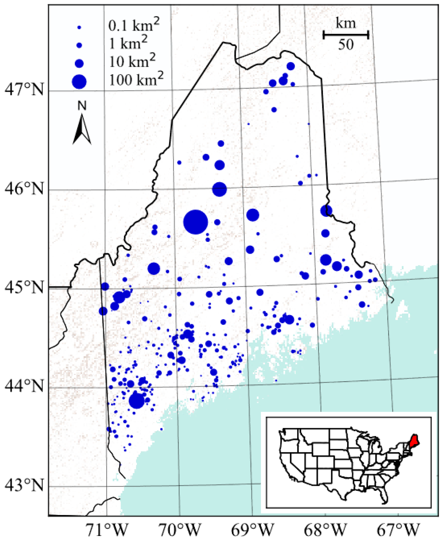
The lakes in this study were selected from HydroLAKES [22], a database providing polygonal boundaries for all global lakes with a surface area of at least 0.1 km2. Additional attributes for each lake include estimates of the shoreline length, average depth, water volume and residence time. Considering the time period of MODIS imagery (from 2000 to current), only lakes with valid in situ lake ice data during the MODIS period were selected. In total, 296 lakes were chosen (shown in Figure 1). The areas of selected lakes range from 0.13 to 305 km2, with the median area of 1.86 km2.
2.2. In Situ and Remote Sensing Data
For validating the remote sensing results, in situ observations which were provided by the Mission of Lake Stewards of Maine (LSM) program were used for comparison (https://www.lakestewardsofmaine.org/). For each lake, the in situ data consists of the name of the lake, nearest town, lake ice breakup and freezeup dates (initial and final). As the observations of initial freezeup dates are too few (22 observations for 18 lakes), only final freezeup dates from remote sensing were validated by comparison with in situ data. There are 292 lakes with in situ breakup data (1890 observations in total) and 112 lakes with freezeup data (427 observations). Individual definitions of lake ice freezeup and breakup timing may vary by observer, which may mean that this is a caveat when interpreting the results of this study [23].
The MOD09GA data product, at a spatial resolution of 1 km, provides a standard cloud mask, including cloud shadows, aerosol quantity, and cirrus detection. The cloud flags were applied to filter out cloudy pixels from reflectance images with heavy cloud cover (see Section 2.3.1). Red reflectance data (841–876 nm, band 1) from the 250 m MODIS/Terra Surface Reflectance Daily product (MOD09GQ, collection 6) [24] from 2000 to 2018 were used to detect ice cover on lake surfaces. Using the red band better constrains the influence from vegetation when mixed pixels are dominant. More details about the reasons for selecting red band instead of the near infrared band, which has been used in past lake and rive ice detection studies [1,15,25] is given in Section 2.3.2.
The Landsat Fmask product was used to calibrate the threshold of MODIS reflectance when classifying ice pixels. The Fmask algorithm was originally developed for masking cloud, cloud shadow, and snow for Landsat TM and ETM+. It classifies pixels into different groups for each individual image using Landsat top of atmosphere reflectance and brightness temperature as inputs based on an object-based cloud and cloud shadow matching algorithm [26]. Using Fmask, we can identify the quality status of the corresponding Landsat pixel (clear, snow, cloud, or cloud shadow) and calculate the ice/snow fraction of a region.
We used temperature data from the Modern-Era Retrospective Analysis for Research and Applications, version 2 (MERRA-2) to identify and remove unreasonably high or low lake ice fraction values during periods of very low or high air temperature, respectively. MERRA-2 is the latest atmospheric reanalysis produced by NASA’s Global Modeling and Assimilation Office [27]. A new glaciated land representation and seasonally varying sea ice albedo have been implemented, leading to improved air temperatures and reduced biases in the net energy flux over these surfaces [28].
2.3. Methods
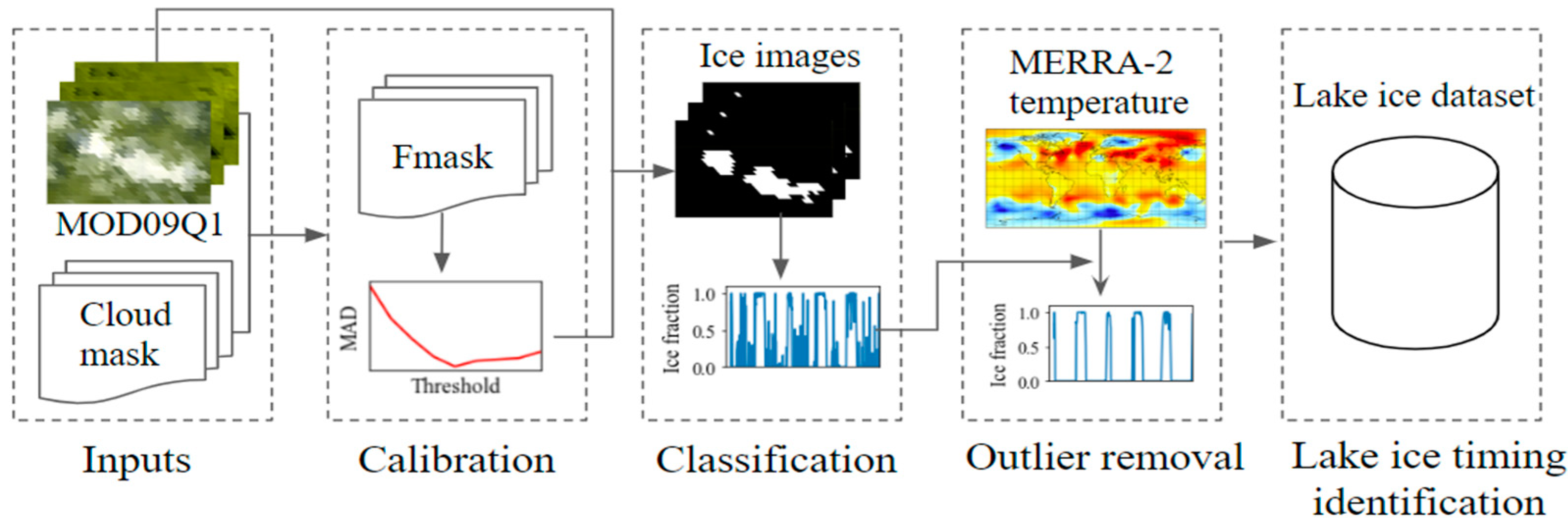
The algorithm for automatically calculating lake ice fraction and detecting lake ice timing contains five major steps is summarized in Figure 2. Firstly, cloud masks were used to remove cloudy pixels from each MODIS reflectance image (Section 2.3.1). Secondly, MODIS images were paired with same-day Landsat Fmask images to find the best reflectance threshold for differentiating ice from water. Thirdly, by counting the number of ice pixels on the ice classification image, the ice fraction over lake surface can be easily estimated and the time series of lake ice fraction is obtained (Section 2.3.2). Fourthly, a quality control operation was taken by using the air temperature data to filter out outliers in the time series of lake ice fraction (Section 2.3.3). Finally, lake breakup and freezeup dates for each lake over the 19-year study period were identified using the time series of lake ice fraction (Section 2.3.4).
2.3.1. Cloud Filtering
The use of optical sensors for ice cover detection is largely limited by clouds. We removed cloud-covered images though using the cloud mask in the state variable band (‘state_1km_1’) of MOD09GA, which is stored in an efficient bit-encoded manner with 16 bits. Each bit represents a different meaning of image quality related status, such as aerosol, clouds, cirrus or cloud shadows. The cloud mask was first resampled to a pixel size of 250 m to make the spatial resolution consistent with MOD09GQ reflectance images. We assigned the same value of each 1000 m pixel to all subpixels (spatial resolution of 250 m). In this study, we only used the most basic digit relevant to clouds, discarding shadows and cirrus. This approach reduced the influence of cloud obstruction while keeping as much information as possible. Images that have more than 70% cloudy pixels were deleted.
2.3.2. Lake Ice Classification and Ice Fraction Calculation
A threshold-based technique was applied to classify satellite reflectance images and to assess the extent of ice coverage. Pixels with red band reflectance values higher than the dynamic threshold (see Section 2.3.3) were classified as ice covered.
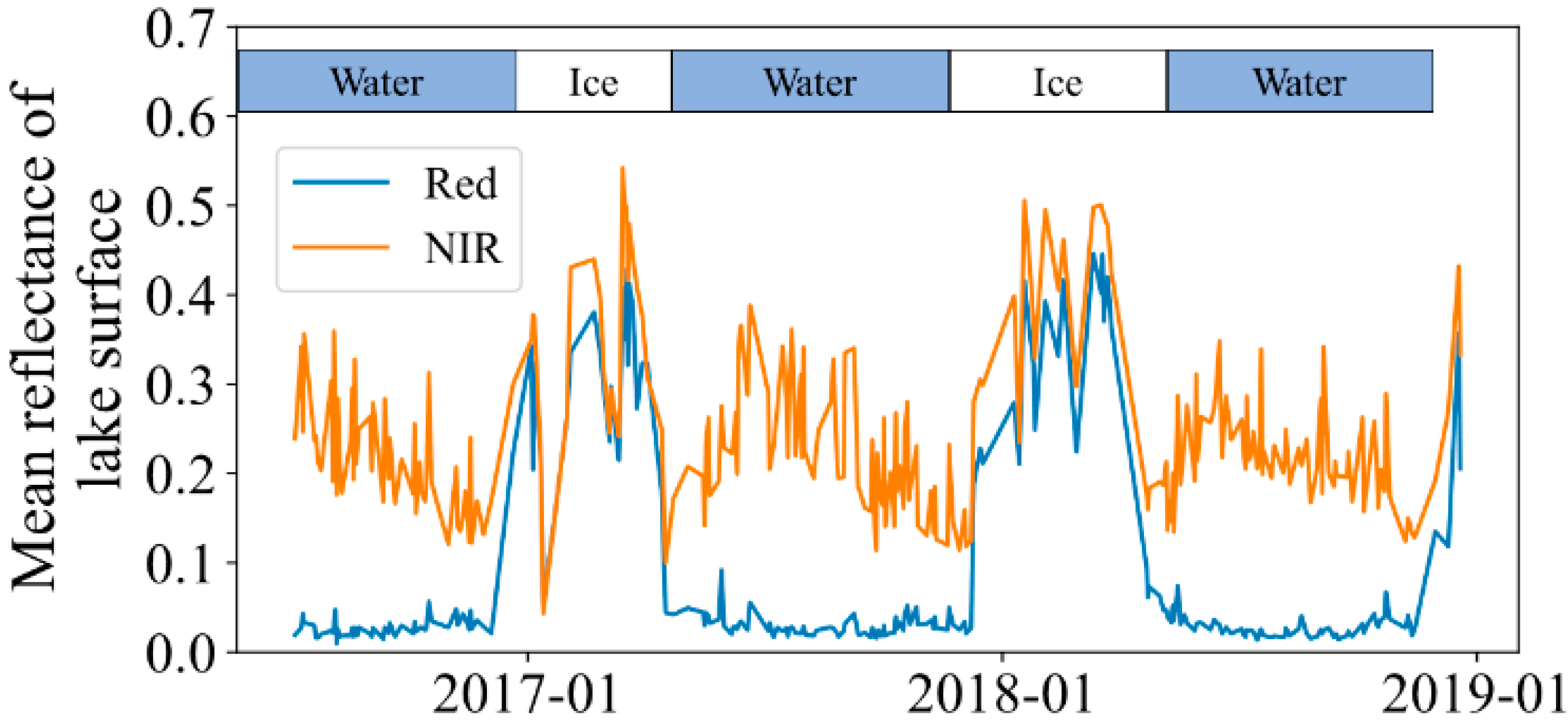
In this study, only the red band was chosen for classification, which is different from the previous studies that used a near-infrared (NIR) band [1,15,25] or the combination of both visible and NIR bands [29,30]. At the scale of MODIS imagery, small lakes are likely to be dominated by mixed pixels that have more than one land cover type. As vegetation has a lower reflectivity in the red band than the NIR band, using the red band to detect lake ice status can better remove the impact of changing vegetation. For example, Figure 3 clearly shows that the signal variation caused by the switch between water and ice in the red band is much clearer than in the NIR band. Due to the greater influence from mixed pixels, NIR reflectance during open water periods is highly relative to red reflectance, which is less vegetation-dependent. As such, it is more difficult to separate ice pixels from water using the NIR band alone. The threshold for classifying ice vs. water was selected by calibrating the lake ice fraction against Landsat Fmask (more details are given in Section 2.3.3).
2.3.3. Calibration Configurations
The classification for each lake was executed multiple times by applying a set of thresholds to MODIS red band imagery. By checking the quality of several classification images visually, we found the best thresholds were roughly around 0.1~0.15. For capturing all optimal thresholds for each individual lake, we set a larger range of thresholds, increasing from 0.06 to 0.18 at an interval of 0.01. The ice fractions were obtained for each threshold. Since we assumed that Landsat Fmask more accurately (see Section 2.2) classifies lake ice cover due to its finer the spatial resolution, the optimal threshold values were calculated by minimizing the mean absolute difference (MAD) between MODIS lake ice fraction and the Landsat Fmask from 2000 to 2018. For each lake, we used this method to estimate a reflectance threshold for ice cover.
2.3.4. Outlier Removal
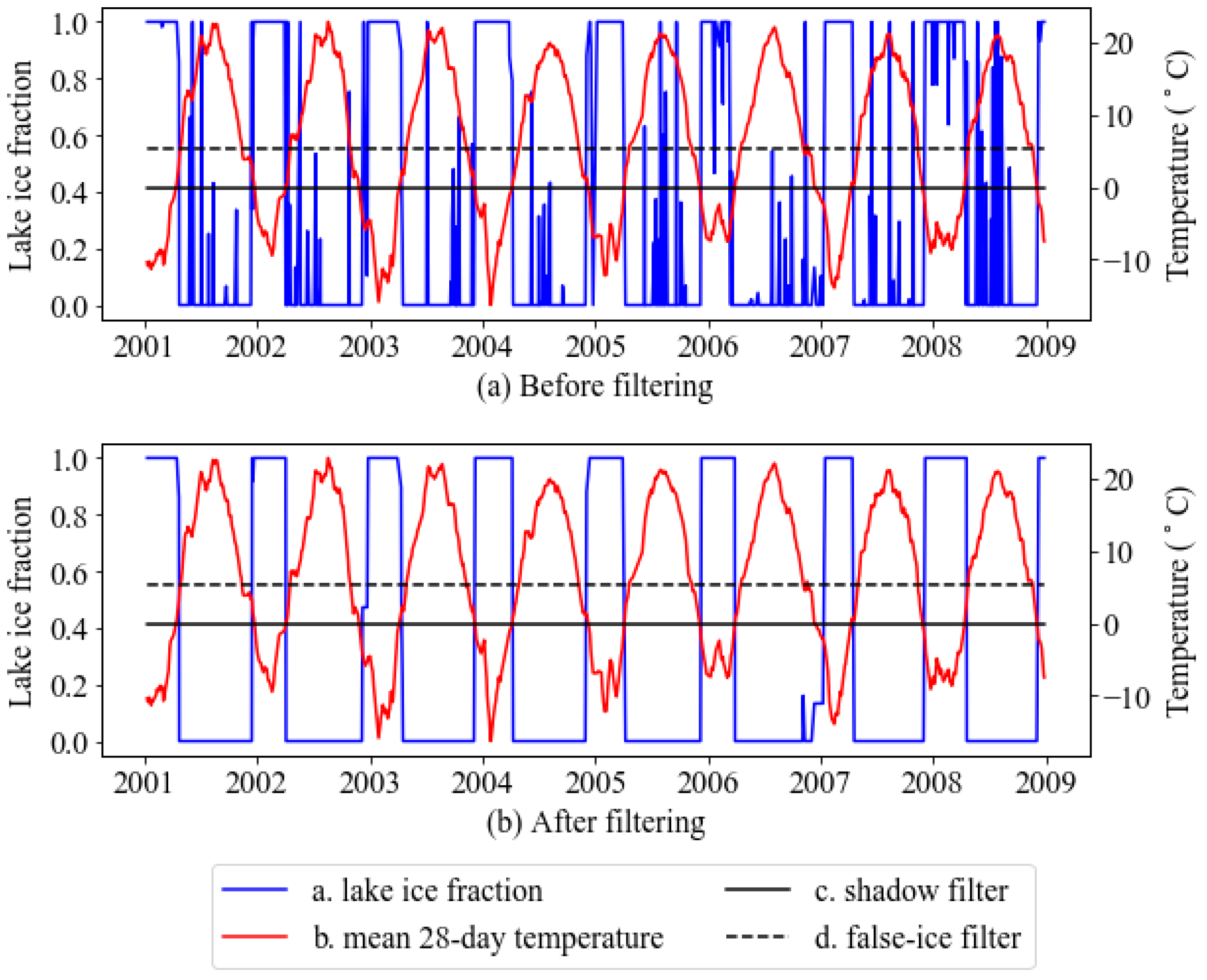
Some factors may result in outliers in the time series of lake ice fraction. One is the presence of topographic shadow, which leads to low reflectance and results in a misclassification of ice as water. Another problem arises from clouds that are not detected by cloud filter. Due to their high reflectance, these clouds are likely to be misclassified as ice. As the variability of lake ice is primarily driven by temperature [14], a relationship between lake ice fraction and the mean daily temperature in the previous N weeks was established through regression. N was set to be 4 weeks (28 days) because the 4-week average temperature has the highest correlation with lake ice fraction in this study (the correlation coefficient between lake ice fraction and average temperatures over 1–6 weeks windows are 0.53, 0.51, 0.56, 0.57, 0.56, 0.55, respectively). A critical value (Tc) of 28-day average temperature for ice formation was selected, corresponding to when lake ice fraction reached 20%. This critical value is called the shadow filter, and it was used for adjusting the underestimation of ice fraction caused by shadows. The assumption is that when temperature is below Tc, no ice should melt and therefore lake ice fraction should not decrease when the temperature is equal or lower than this critical value. Based on this assumption, the underestimation of ice fraction on the ith day caused by shadow can be corrected according to Equation (1), where F is the ice fraction, T is the mean temperature, and i − 1 is the previous day of the ith day.
The other filter based on temperature data is called false-ice filter. It reduced the false detection of ice cover caused by clouds by Equation (2).
The principle of false-ice filter is that when 28-day mean temperature was greater than the threshold identified by the false-ice filter, we assumed that lake ice fraction should not increase, and we set to ice cover on the previous day (Figure 4). The false-ice filter equals Tc plus one standard deviation of the mean temperature when the lake was partially frozen (ice fraction is within 20% to 80%).
2.3.5. Identification of Breakup and Freezeup Dates
We identified the timing of freezeup and breakup based on thresholds in lake ice fraction. For consistency with in situ data, the breakup date was defined as the start of thawing and the freezeup date is defined as the end of freezing. The thresholds of 20% and 80% were used to identify breakup and freezeup timing, respectively. When the lake ice fraction first dropped below 20% each spring, we identified the breakup date. Similarly, the freezeup date was defined as the first day each fall when the lake ice fraction exceeded 80%. The 20% and 80% thresholds allow for some error caused by misclassification of cloud as ice.
2.3.6. Spatial Variability and Correlation of Lake Ice Timing
We examined the spatial correlation of lake ice timing by using semivariogram analysis [31] (Figure 8) for both results from the proposed algorithm and in situ data. Since the extent of in situ data is not consistent for each year, we selected 2017 to test the spatial auto-correlation of lake ice timing based on the fact that 2017 had the most observations during the study period. In total, there were 54 observations of freezeup and 141 breakups in situ observations. The equation for calculating semi-variance is shown in Equation (3).
where N(h) is the number of pairs for distance h, z(u) is the lake ice phenology timing at position u.
3. Results
3.1. Calibration Results
We calibrated the thresholds for the classification algorithm as described in Section 2.3.3 by comparing MODIS-based lake ice fraction estimates with comparable values from Fmask. The minimal MAD values for all lakes are shown in Figure 5a. We subdivided our sample of 296 lakes into three groups depending on the lake surface areas. Lakes with surface areas smaller than 0.5 km2 were labeled as the small group. Lakes in medium group were from 0.5 to 1 km2. Lakes larger than 1 km2 were in the large group. The mean MAD values for small, medium and large lakes were 2.05%, 1.95% and 2.13%, respectively. The similarity of these values suggests that the classification algorithm may perform well for lakes of all sizes as appropriate thresholds are selected.
The thresholds are controlled by multiple factors such as water turbidity, fraction of non-water pixels and types of non-water pixels. For example, the reflectance of a mixed pixel containing vegetation could be quite different from pixels containing high-reflectance land-type such as urban area. The optimal thresholds selected for lakes ranges from 0.07 to 0.17 (Figure 5b). The most common thresholds were 0.11, 0.12 and 0.13. They were identified for 54, 54, and 55 lakes, respectively. Lakes with thresholds from 0.11 to 0.13 accounted for 55% of the total lakes. To test their temporal stability, we also calibrated the thresholds during three subsets (2000–2005, 2006–2011, 2012–2018) of the study period. Slight variations of the thresholds were detected. The mean absolute difference between the thresholds calibrated during the whole period and the thresholds which were calibrated during the three sub-periods were 0.011, 0.013 and 0.013, respectively, which suggests the thresholds were relatively stable during the study period.
3.2. Validation of Remotely Sensed Lake Ice Timing
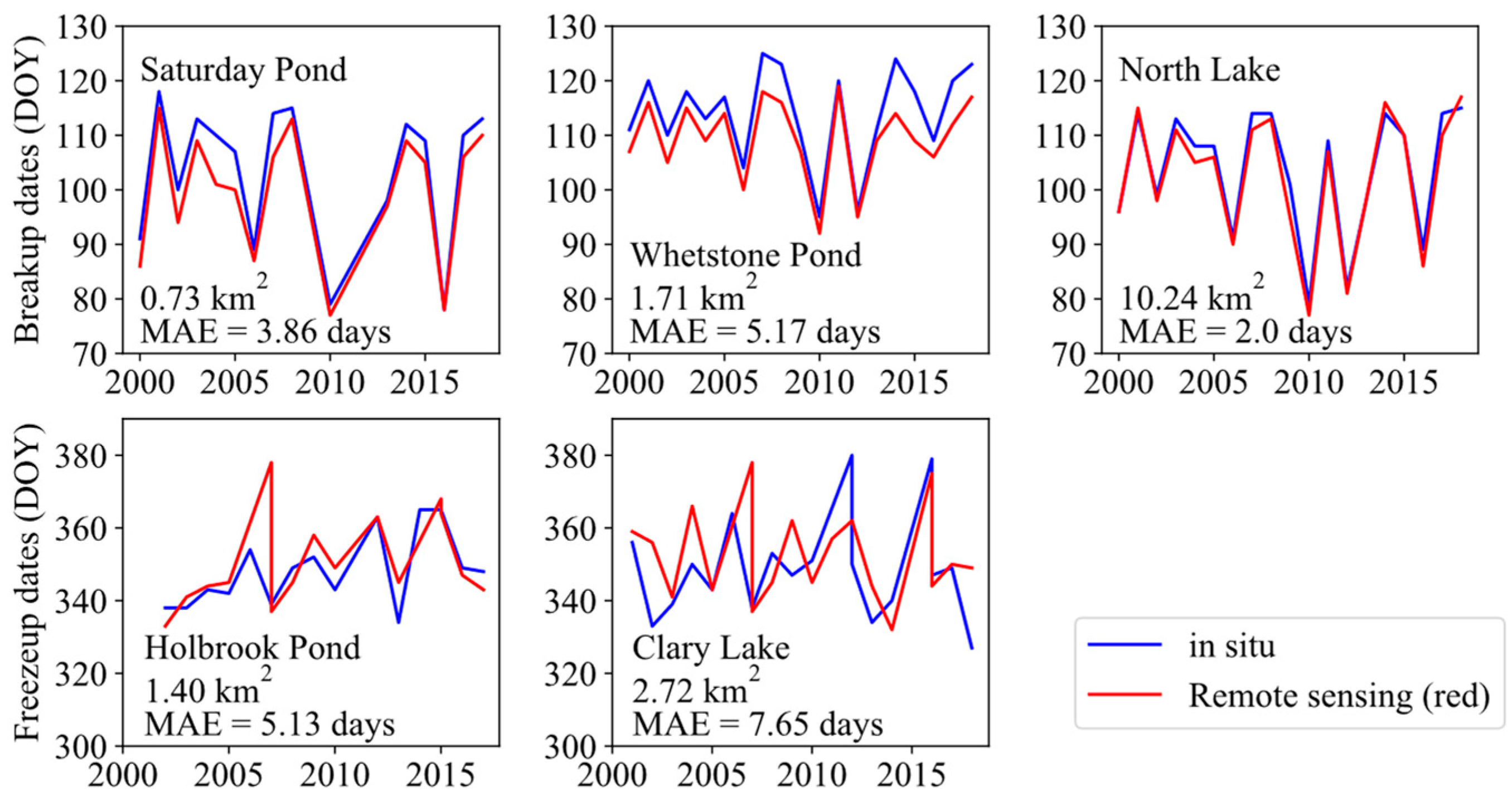
The time series of breakup and freezeup over lakes with full records of in situ data show strong similarities when measured using in situ and remotely sensed approaches (Figure 6). Due to incomplete in situ data, only three lakes have complete breakup records and two lakes have full freezeup records (no missing data from 2000 to 2018). As shown in Figure 6, the variability of lake ice timing was generally captured well by the remote sensing approach. There was a good agreement between remotely sensed breakup dates with in situ observation. However, larger bias existed in the time series of freezeup, especially for Clary Lake, where a 20-day difference was found in 2012.
3.2.1. Validation of Breakup Dates
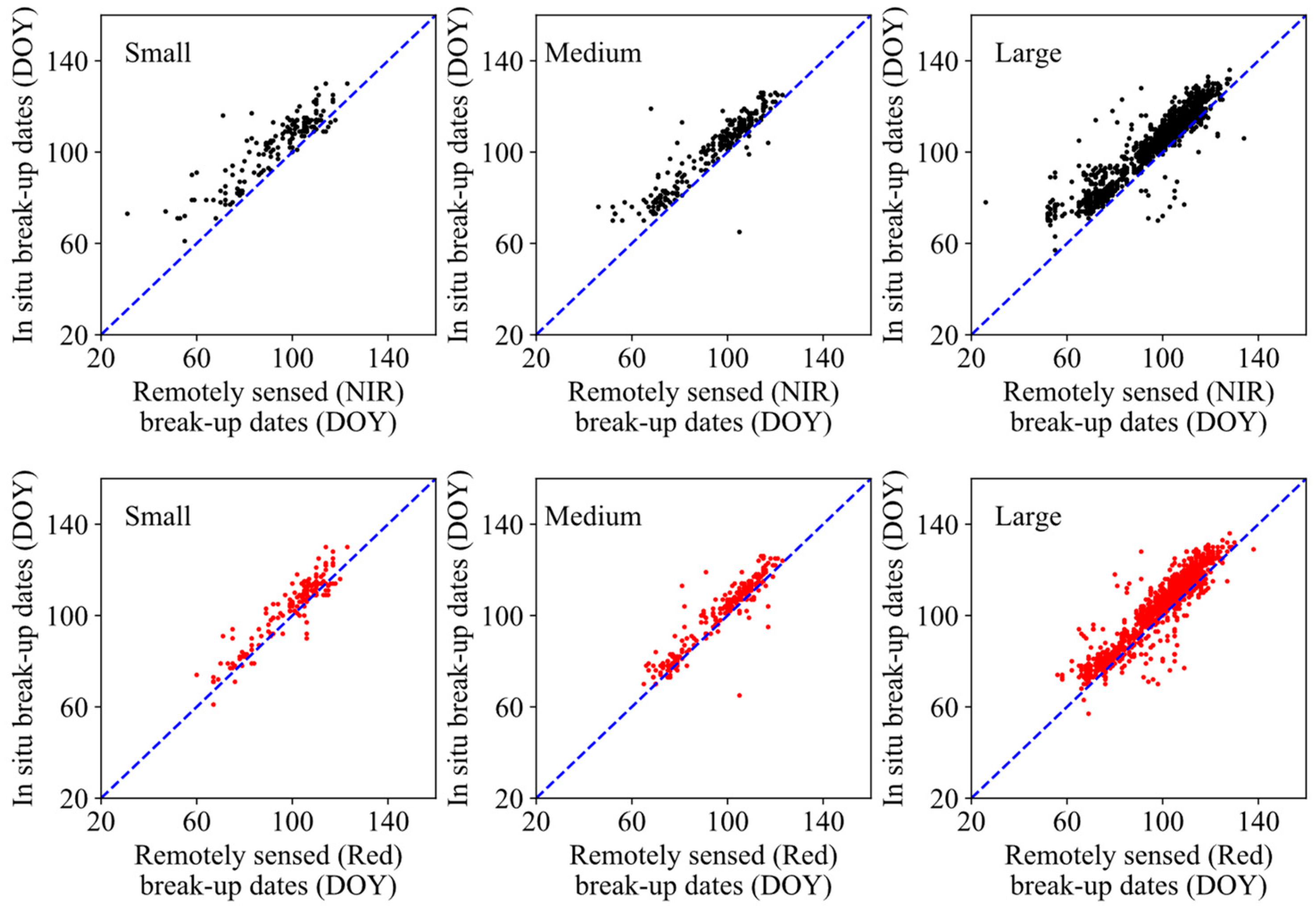
To better understand the characteristics of the proposed algorithm, we comprehensively validated it by comparing the results with in situ data and the method proposed by [25] which is based on the NIR band (referred as “remote sensing NIR”).
The comparison of breakup dates with in-situ data (Figure 7) for each group shows that the breakup dates were detected with relatively high accuracy for lakes of all sizes. The overall mean absolute error (MAE), correlation coefficient (r) and bias were 5.54 days, 0.92 and −4.4 days, respectively for the proposed algorithm. The mean bias of the proposed algorithm was −3.79 days for small lakes, −3.41 days for medium lakes and −4.31 days for large lakes. The negative biases found in all groups indicate that the breakup dates detected by remote sensing methods were earlier than the in situ observations. We suggest two possible reasons: firstly, the definition of breakup dates of MODIS-based approach (<20% lake ice fraction) may differ from that of ground-based observers. The difference might be even larger for large lakes since what remote sensing observed is the overview of lake ice status while humans can only infer the lake ice phenology of whatever fraction of a lake can be observed from shore. This difference may partially explain why the largest bias was obtained for larger lakes. Secondly, thin ice or ice with low albedo due to melt season processes might be detected as water by MODIS during the breakup period. The mean MAE values for three groups were 5.06 days, 5.00 days and 5.70 days. The mean normalized root mean square errors (NRMSE) were 5.51 days, 5.70 days and 6.41 days. Results for all three groups of lakes were quite similar. The error statistics suggest that the MODIS-based approach captured the lake ice breakup dates accurately for lakes of all sizes tested here.
The red band method outperformed the NIR-based algorithm [25] in all cases (Table 1, Figure 7). Taking the MAE of breakup dates as an example, the red band algorithm led to an improvement over the NIR-based algorithms of 3.39, 3.78 and 2.86 days for the small, medium and large groups, respectively. This result suggests that the red band algorithm performed well for lakes of all sizes, and small and medium lakes improved even more so. As explained in Section 2, two of the key differences of these two algorithms are the red band used and the self-adjust threshold of classification over each individual lake. This result leads more pixels to be classified accurately, resulting in breakup dates detected with higher accuracy. Another difference is the use of temperature filters, which could remove the outliers of erroneously detected freezeup or breakup events caused by clouds and clouds/topographic shadows.
3.2.2. Validation of Freezeup Dates
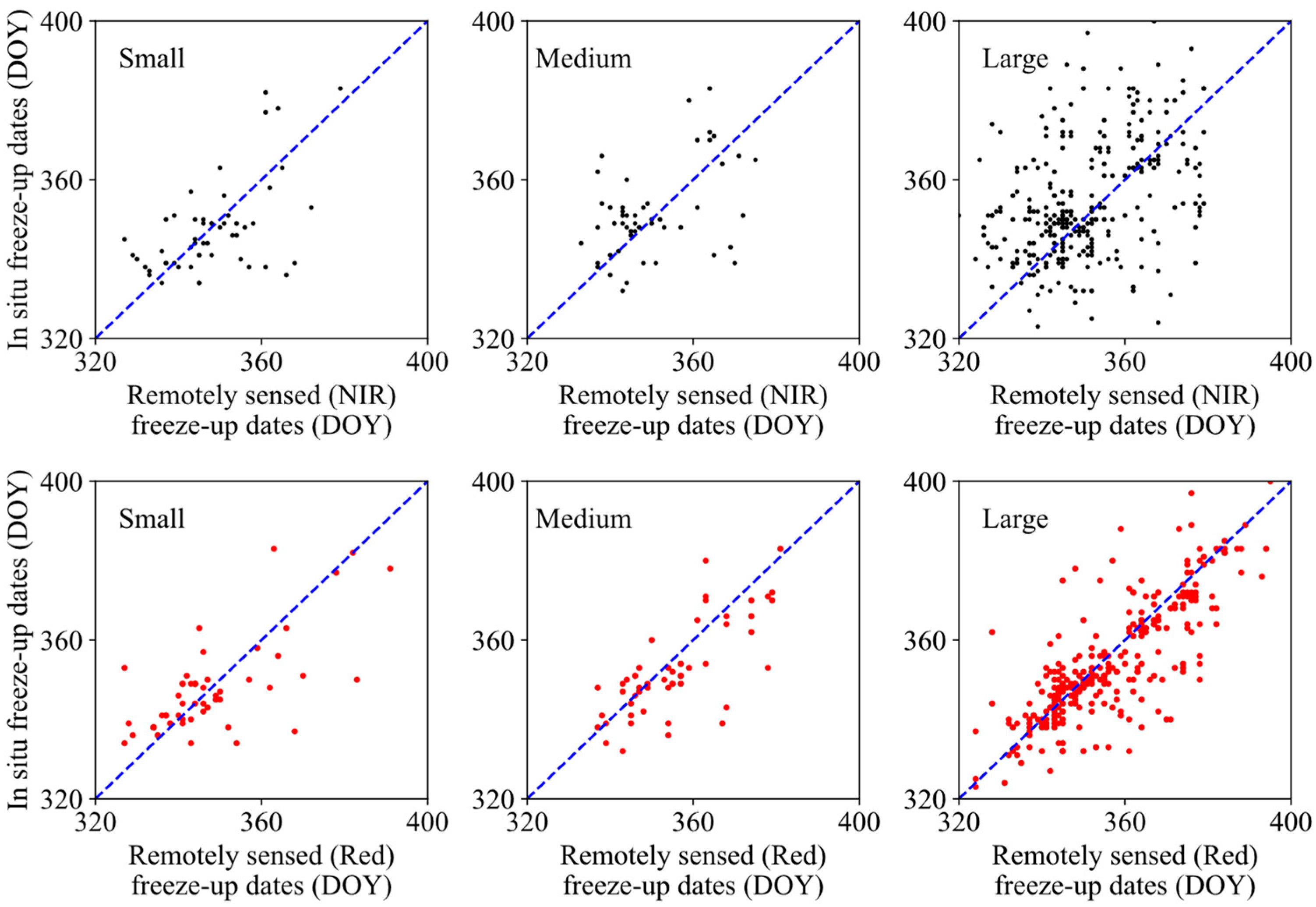
When detecting freezeup, the overall MAE, r and bias of the proposed algorithm were 7.31 days, 0.77 and 3.33 days, respectively, across all groups (Figure 8). The biases of the proposed algorithm for small, medium and large lakes were −1.06 days, 3.58 days and 2.48 days, respectively. Unlike breakup dates, freezeup dates detected from MODIS showed negative bias for small lakes but positive bias for medium and large lakes. As with breakup, inconsistency between remote sensing results and in situ observations might be caused by either differences in the definition of lake ice freezeup or the presence of clear ice that is not easy to observe accurately using optical sensors. The mean MAE values for small, medium, and large lakes are 7.40 days, 8.27 days and 5.99 days, respectively. The NRMSEs are 8.74 days, 9.20 days and 7.08 days.
Compared with the NIR-based algorithm, the proposed algorithm outperformed in all cases except bias in small and medium groups. Although a higher bias in the case of the red band method suggests lower accuracy, a low MAE and NRMSE mean the absolute value of freezeup dates detected by the proposed algorithm were closer to in situ observations.
3.3. Spatial Variability and Correlation of Lake Ice Timing
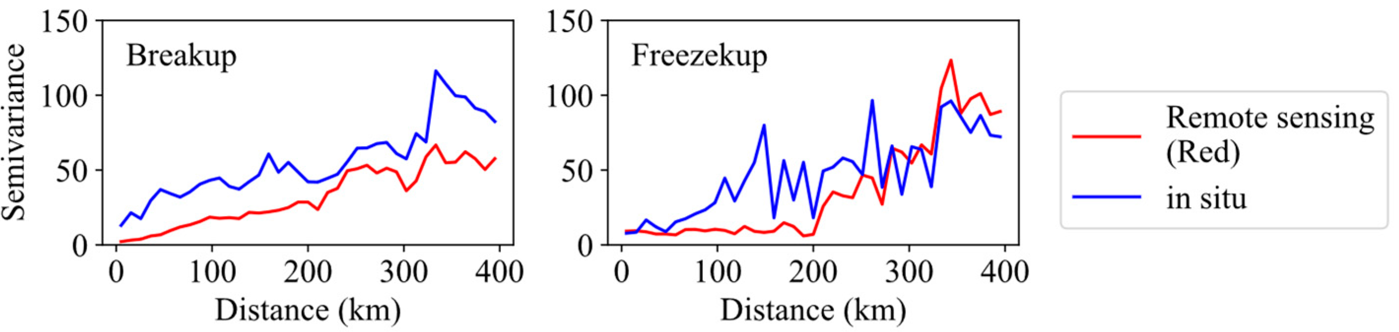
The semivariance increased as the distance between measured locations became longer for both breakup and freezeup dates (Figure 9). This indicate a general pattern in which closer lakes have more similar ice breakup and freezeup dates. Though the semivariance of both remote sensing and in situ lake ice timing show a positive trend when distances increase, there is an obvious difference between them. In general, the semivairance of in situ is greater than remote sensing-based results by 46.97 and 21.0 for breakup and freezeup, respectively. The larger variance of in situ lake ice timing may be explained by two possible reasons. Firstly, the remotely sensed lake ice observation method is more consistent, removing the influence of human interpretation. Secondly, spatial differences in lake ice timing may be difficult to capture using remote sensing in some cases due to dark and thin surface ice or snow coverage around small lakes, making the remotely sensed semivaiance smaller than in situ.
Semivariograms generated from in situ and remote sensing data do not show clear sills, suggesting that characteristic length scales at which lake ice phenology covaries are larger than those tested here. The increases in semivariance with spatial scale are similar for in situ and remotely sensed observations, however, which suggests that they are capturing the same general patterns of spatial covariability.
4. Discussion
This algorithm can produce lake ice products to support the research of interactions between lakes and biogeochemical, limnological and ecological regimes over large spatial scales. For instance, According to [7], the processing of dissolved organic carbon in arctic fresh water is controlled by photoreactions. Earlier breakup dates could increase the absorption of solar radiation and therefore accelerate the releasing of carbon from water to atmosphere. A comprehensive ice phenology dataset covering lakes in all sizes would be beneficial to better understand the fate of carbon in the Arctic. In addition, changes in ice duration may impact lake evaporation in high-latitude regions [32]. Ice coverage information from the proposed algorithm can lead to a more accurate evaporation calculation over the majority of boreal lakes. This algorithm could also be used for identifying ice covered lakes in other satellite datasets. For example, the Surface Water Ocean Topography (SWOT) mission aims at measuring variations in area and water surface elevation of for the majority of water bodies all over the world [33]. Lakes as small as 0.0625 km2 globally will be estimated by SWOT mission. As it is uncertain whether SWOT’s Ka-band radar can detect ice automatically, and current lake ice datasets at large spatial scale only focus lakes large than 1 km2, the development of a global ice cover dataset using the approach proposed in this study would help ensure the consistency of SWOT datasets.
Nonetheless, this algorithm still has some limitations. Firstly, because it solely depends on optical satellite images, lake ice estimations from satellite are unavailable when severe cloud contamination exists. For regions with heavy clouds, remotely sensed lake ice phenology dates have high uncertainties and may be biased due to missing data. Secondly, the 19-year length of the data record is relatively short for analyzing trends. We calculated the trends for lake breakup and freezeup using Sen’s slope [34] and Mann-Kendall test [35,36]. There were only 3% of lakes with significant breakup trends and 2.10% of lakes with significant freezeup trend (p < 0.05). The short length of data may be one of the reasons that only a few lakes have significant trends. Also, as the algorithm is based on moderate spatial resolution imagery, the results may be biased in some specific cases. For example, if a small lake has not started freezing while the surrounding area is already covered by snow, the lake might be mistaken as frozen/partial frozen since the MODIS red reflectance value would be high in mixed pixels. The snow cover in mixed pixels might explain why negative bias in freezeup date was detected for small lakes while positive freezeup bias was observed for medium and large lakes. While we do not observe systematic problems of this nature in our test dataset, it may account for errors in some individual lakes. In addition, the gridded MODIS product that we used was mapped from MODIS swath pixels. When multiple pixels of MODIS swath data were overlapped in a MODIS grid, only the “most relevant pixel” was selected according to [37], which might be another source of bias caused by this gridding operation.
5. Conclusions
In this study, a new method was developed to estimate lake ice timing over a range of lake sizes by combing MODIS, Landsat Fmask, and an air temperature filter from MERRA-2 to remove outliers. Differing from the previous studies that used a near-infrared (NIR) band [1,15,25] or the combination of both visible and NIR [29,30,38], only the red band was used to remove the impact of changing vegetation. Validation results against in situ observations over lakes of different sizes suggest that the approach performs well for all lakes. The MAE of breakup dates were 5.06 days, 5.0 days and 5.70 days for small, medium and large lakes. For freezeup dates, the MAE were 7.4 days, 8.27 days and 5.99 days for lakes in small, medium and large groups. Results indicate that there were no substantial differences among lakes with different surface areas.
This method makes new contributions to lake ice remote sensing in several ways. Firstly, it is the first time that red reflectance band of MODIS and Landsat Fmask have been used in combination for identifying lake ice timing. The combined use of Landsat Fmask and MODIS red reflectance has alleviated the limitation of the mixed pixel issue related to low spatial resolution relative to lake size. Secondly, the filtering operation based on air temperature data was used for filtering the outliers of lake ice fraction time series which alleviated the influence from topographic shadow and clouds which are not detected by cloud masks. Thirdly, the capability to measure ice phenology for lakes as small as ~0.1 km2 substantially increases the number of lakes that can be observed. By applying the lake ice monitoring algorithm presented here to global lakes, a lake ice dataset with much greater spatial representativeness could be established.
Author Contributions
Funding acquisition, T.P.; Methodology, S.Z.; Supervision, T.P.; Writing–original draft, S.Z.; Writing–review & editing, T.P.
Funding
This work was funded by a subcontract from the SWOT Project at the NASA/Caltech Jet Propulsion Lab.
Acknowledgments
We would like to thank the Mission of Lake Stewards of Maine (LSM) program for providing the in situ lake ice observations.
Conflicts of Interest
The authors declare no conflict of interest.
References
- Latifovic, R.; Pouliot, D. Analysis of climate change impacts on lake ice phenology in Canada using the historical satellite data record. Remote Sens. Environ. 2007, 106, 492–507. [Google Scholar] [CrossRef]
- Magnuson, J.J.; Robertson, D.M.; Benson, B.J.; Wynne, R.H.; Livingstone, D.M.; Arai, T.; Assel, R.A.; Barry, R.G.; Card, V.; Kuusisto, E. Historical trends in lake and river ice cover in the Northern Hemisphere. Science 2000, 289, 1743–1746. [Google Scholar] [CrossRef] [PubMed]
- Adrian, R.; O’Reilly, C.M.; Zagarese, H.; Baines, S.B.; Hessen, D.O.; Keller, W.; Livingstone, D.M.; Sommaruga, R.; Straile, D.; Van Donk, E. Lakes as sentinels of climate change. Limnol. Oceanogr. 2009, 54, 2283–2297. [Google Scholar] [CrossRef] [PubMed]
- Duguay, C.R.; Flato, G.M.; Jeffries, M.O.; Ménard, P.; Morris, K.; Rouse, W.R. Ice-cover variability on shallow lakes at high latitudes: Model simulations and observations. Hydrol. Process. 2003, 17, 3465–3483. [Google Scholar] [CrossRef]
- Duguay, C.R.; Prowse, T.D.; Bonsal, B.R.; Brown, R.D.; Lacroix, M.P.; Ménard, P. Recent trends in Canadian lake ice cover. Hydrol. Process. Int. J. 2006, 20, 781–801. [Google Scholar] [CrossRef]
- Wang, W.; Lee, X.; Xiao, W.; Liu, S.; Schultz, N.; Wang, Y.; Zhang, M.; Zhao, L. Global lake evaporation accelerated by changes in surface energy allocation in a warmer climate. Nat. Geosci. 2018, 11, 410–414. [Google Scholar] [CrossRef]
- Cory, R.M.; Ward, C.P.; Crump, B.C.; Kling, G.W. Sunlight controls water column processing of carbon in arctic fresh waters. Science 2014, 345, 925–928. [Google Scholar] [CrossRef]
- Che, T.; Li, X.; Jin, R. Monitoring the frozen duration of Qinghai Lake using satellite passive microwave remote sensing low frequency data. Chin. Sci. Bull. 2009, 54, 2294–2299. [Google Scholar] [CrossRef]
- Brakenridge, G.R.; Nghiem, S.V.; Anderson, E.; Mic, R. Orbital microwave measurement of river discharge and ice status. Water Resour. Res. 2007, 43. [Google Scholar] [CrossRef]
- Duguay, C.; Lafleur, P. Determining depth and ice thickness of shallow sub-Arctic lakes using space-borne optical and SAR data. Int. J. Remote Sens. 2003, 24, 475–489. [Google Scholar] [CrossRef]
- Jeffries, M.; Morris, K.; Liston, G. A method to determine lake depth and water availability on the North Slope of Alaska with spaceborne imaging radar and numerical ice growth modelling. Arctic 1996, 49, 367–374. [Google Scholar] [CrossRef]
- Wakabayashi, H.; Weeks, W.; Jeffries, M.O. A C-band backscatter model for lake ice in Alaska. In Proceedings of the IGARSS′93-IEEE International Geoscience and Remote Sensing Symposium, Tokyo, Japan, 18–21 August 1993; pp. 1264–1266. [Google Scholar]
- Nolan, M.; Liston, G.; Prokein, P.; Brigham-Grette, J.; Sharpton, V.L.; Huntzinger, R. Analysis of lake ice dynamics and morphology on Lake El’gygytgyn, NE Siberia, using synthetic aperture radar (SAR) and Landsat. J. Geophys. Res. Atmos. 2002, 107, ALT 3-1–ALT 3-12. [Google Scholar] [CrossRef]
- Arp, C.D.; Jones, B.M.; Grosse, G. Recent lake ice-out phenology within and among lake districts of Alaska, USA. Limnol. Oceanogr. 2013, 58, 2013–2028. [Google Scholar] [CrossRef]
- Šmejkalová, T.; Edwards, M.E.; Dash, J. Arctic lakes show strong decadal trend in earlier spring ice-out. Sci. Rep. 2016, 6, 38449. [Google Scholar] [CrossRef] [PubMed]
- Wang, J. Alaskan Lake Database Mapped from Landsat Images. Version 1.0. UCAR/NCAR-Earth Observing. 2011. Available online: https://0-doi-org.brum.beds.ac.uk/10.5065/D6MC8X5R (accessed on 12 December 2018).
- Rouse, W.R.; Blanken, P.D.; Duguay, C.R.; Oswald, C.J.; Schertzer, W.M. Climate-lake interactions. In Cold Region Atmospheric and Hydrologic Studies. The Mackenzie GEWEX Experience; Woo, M., Ed.; Springer: Berlin, Germany, 2008; pp. 139–160. [Google Scholar]
- Brown, L.C.; Duguay, C.R. The response and role of ice cover in lake-climate interactions. Prog. Phys. Geogr. 2010, 34, 671–704. [Google Scholar] [CrossRef]
- Adrian, R.; Walz, N.; Hintze, T.; Hoeg, S.; Rusche, R. Effects of ice duration on plankton succession during spring in a shallow polymictic lake. Freshw. Biol. 1999, 41, 621–634. [Google Scholar] [CrossRef]
- Foga, S.; Scaramuzza, P.L.; Guo, S.; Zhu, Z.; Dilley, R.D.; Beckmann, T.; Schmidt, G.L.; Dwyer, J.L.; Hughes, M.J.; Laue, B. Cloud detection algorithm comparison and validation for operational Landsat data products. Remote Sens. Environ. 2017, 194, 379–390. [Google Scholar] [CrossRef] [Green Version]
- Shao, Z.; Hou, J.; Jiang, M.; Zhou, X. Cloud detection in Landsat imagery for Antarctic region using multispectral thresholds. In Proceedings of the Remote Sensing of the Atmosphere, Clouds, and Precipitation V, International Society for Optics and Photonics, Beijing, China, 8 November 2014; Volume 9259. [Google Scholar]
- Messager, M.L.; Lehner, B.; Grill, G.; Nedeva, I.; Schmitt, O. Estimating the volume and age of water stored in global lakes using a geo-statistical approach. Nat. Commun. 2016, 7, 13603. [Google Scholar] [CrossRef]
- Hodgkins, G.A.; James, I.C.; Huntington, T.G. Historical changes in lake ice-out dates as indicators of climate change in New England, 1850–2000. Int. J. Climatol. A J. R. Meteorol. Soc. 2002, 22, 1819–1827. [Google Scholar] [CrossRef]
- Vermote, E.; Kotchenova, S.; Ray, J. MODIS Surface Reflectance User’s Guide; The Land Surface Reflectance Science Computing Facility: Greenbelt, MD, USA, 2011; pp. 1–35. [Google Scholar]
- Cooley, S.W.; Pavelsky, T.M. Spatial and temporal patterns in Arctic river ice breakup revealed by automated ice detection from MODIS imagery. Remote Sens. Environ. 2016, 175, 310–322. [Google Scholar] [CrossRef]
- Zhu, Z.; Wang, S.; Woodcock, C.E. Improvement and expansion of the Fmask algorithm: Cloud, cloud shadow, and snow detection for Landsats 4–7, 8, and Sentinel 2 images. Remote Sens. Environ. 2015, 159, 269–277. [Google Scholar] [CrossRef]
- Gelaro, R.; McCarty, W.; Suárez, M.J.; Todling, R.; Molod, A.; Takacs, L.; Randles, C.A.; Darmenov, A.; Bosilovich, M.G.; Reichle, R. The modern-era retrospective analysis for research and applications, version 2 (MERRA-2). J. Clim. 2017, 30, 5419–5454. [Google Scholar] [CrossRef]
- Cullather, R.I.; Nowicki, S.M.; Zhao, B.; Suarez, M.J. Evaluation of the surface representation of the Greenland Ice Sheet in a general circulation model. J. Clim. 2014, 27, 4835–4856. [Google Scholar] [CrossRef]
- Pavelsky, T.M.; Smith, L.C. Spatial and temporal patterns in Arctic river ice breakup observed with MODIS and AVHRR time series. Remote Sens. Environ. 2004, 93, 328–338. [Google Scholar] [CrossRef]
- Beaton, A.; Whaley, R.; Corston, K.; Kenny, F. Identifying historic river ice breakup timing using MODIS and Google Earth Engine in support of operational flood monitoring in Northern Ontario. Remote Sens. Environ. 2019, 224, 352–364. [Google Scholar] [CrossRef]
- Karl, J.W.; Maurer, B.A. Spatial dependence of predictions from image segmentation: A variogram-based method to determine appropriate scales for producing land-management information. Ecol. Inform. 2010, 5, 194–202. [Google Scholar] [CrossRef]
- Zhao, G.; Gao, H. Estimating reservoir evaporation losses for the United States: Fusing remote sensing and modeling approaches. Remote Sens. Environ. 2019, 226, 109–124. [Google Scholar] [CrossRef] [Green Version]
- Biancamaria, S.; Lettenmaier, D.P.; Pavelsky, T.M. The SWOT mission and its capabilities for land hydrology. Surv Geophys. 2016, 37, 117–147. [Google Scholar] [CrossRef]
- Sen, P.K. Estimates of the regression coefficient based on Kendall’s tau. J. Am. Stat. Assoc. 1968, 63, 1379–1389. [Google Scholar] [CrossRef]
- Mann, H.B. Non-parametric tests against trend. Econometrica 1945, 13, 163–171. [Google Scholar] [CrossRef]
- Kendall, M.G. Rank Correlation Methods; Griffin: Oxford, UK, 1948. [Google Scholar]
- Wolfe, R.E.; Roy, D.P.; Vermote, E. MODIS land data storage, gridding, and compositing methodology: Level 2 grid. IEEE Trans. Geosci. Remote Sens. 1998, 36, 1324–1338. [Google Scholar] [CrossRef] [Green Version]
- Yang, K.; Smith, L.C. Supraglacial streams on the Greenland Ice Sheet delineated from combined spectral–shape information in high-resolution satellite imagery. IEEE Geosci. Remote Sens. Lett. 2012, 10, 801–805. [Google Scholar] [CrossRef]
Figure 1.
Locations of study lakes in Maine.

Figure 2.
Flow chart of the algorithm.

Figure 3.
Mean reflectance of near infrared (NIR) and red band over surface of Silver Lake (Figure 8, Pond) lake in Maine. Two periods of water and ice are labelled.
Figure 3.
Mean reflectance of near infrared (NIR) and red band over surface of Silver Lake (Figure 8, Pond) lake in Maine. Two periods of water and ice are labelled.

Figure 4.
Time series of lake ice fraction and temperature over Silver Lake (a) before and (b) after filtering.
Figure 4.
Time series of lake ice fraction and temperature over Silver Lake (a) before and (b) after filtering.

Figure 5.
Calibration of MODIS thresholds against lake fraction of Landsat Fmask. (a) is the mean absolute distance (MAD) between MODIS and Fmask lake ice fraction calculated using the optimal thresholds. Lakes are divided into three groups by size. (b) is the distribution of optimal thresholds selected by all lakes.

Figure 6.
Time series of lake ice breakup and freezeup dates.

Figure 7.
Validation results for breakup dates.

Figure 8.
Validation results of freezeup dates. Freezeup dates later than day 365 (or 366 days in a leap year) means freezeup was detected in the following year.
Figure 8.
Validation results of freezeup dates. Freezeup dates later than day 365 (or 366 days in a leap year) means freezeup was detected in the following year.

Figure 9.
Semivariogram of breakup and freezeup dates in 2017.


Table 1.
Statistical validation results for the remotely sensed lake ice breakup and freezeup dates.
Table 1.
Statistical validation results for the remotely sensed lake ice breakup and freezeup dates.
| Breakup | Freezeup | |||
|---|---|---|---|---|
| NIR | Red | NIR | Red | |
| Small | ||||
| Bias | −8.23 | −3.79 | −0.96 | −1.0 |
| MAE | 8.45 | 5.06 | 8.47 | 7.40 |
| NRMSE | 9.36 | 5.51 | 10.49 | 8.74 |
| Medium | ||||
| Bias | −8.24 | −3.41 | −2.97 | 3.5 |
| MAE | 8.78 | 5.0 | 11.96 | 8.27 |
| NRMSE | 9.68 | 5.70 | 12.86 | 9.20 |
| Large | ||||
| Bias | −6.68 | −4.31 | −3.38 | 2.4 |
| MAE | 7.37 | 5.70 | 11.76 | 5.99 |
| NRMSE | 8.37 | 6.41 | 13.02 | 7.08 |
© 2019 by the authors. Licensee MDPI, Basel, Switzerland. This article is an open access article distributed under the terms and conditions of the Creative Commons Attribution (CC BY) license (http://creativecommons.org/licenses/by/4.0/).
Share and Cite
MDPI and ACS Style
Zhang, S.; Pavelsky, T.M. Remote Sensing of Lake Ice Phenology across a Range of Lakes Sizes, ME, USA. Remote Sens. 2019, 11, 1718. https://0-doi-org.brum.beds.ac.uk/10.3390/rs11141718
AMA Style
Zhang S, Pavelsky TM. Remote Sensing of Lake Ice Phenology across a Range of Lakes Sizes, ME, USA. Remote Sensing. 2019; 11(14):1718. https://0-doi-org.brum.beds.ac.uk/10.3390/rs11141718
Chicago/Turabian StyleZhang, Shuai, and Tamlin M. Pavelsky. 2019. "Remote Sensing of Lake Ice Phenology across a Range of Lakes Sizes, ME, USA" Remote Sensing 11, no. 14: 1718. https://0-doi-org.brum.beds.ac.uk/10.3390/rs11141718
Note that from the first issue of 2016, this journal uses article numbers instead of page numbers. See further details here.