Advantages of Geostationary Satellites for Ionospheric Anomaly Studies: Ionospheric Plasma Depletion Following a Rocket Launch

Abstract

In this study, we analyzed signals transmitted by the U.S. Wide Area Augmentation System (WAAS) geostationary (GEO) satellites using the Variometric Approach for Real-Time Ionosphere Observation (VARION) algorithm in a simulated real-time scenario, to characterize the ionospheric response to the 24 August 2017 Falcon 9 rocket launch from Vandenberg Air Force Base in California. VARION is a real-time Global Navigation Satellites Systems (GNSS)-based algorithm that can be used to detect various ionospheric disturbances associated with natural hazards, such as tsunamis and earthquakes. A noise reduction algorithm was applied to the VARION-GEO solutions to remove the satellite-dependent noise term. Our analysis showed that the interactions of the exhaust plume with the ionospheric plasma depleted the total electron content (TEC) to a level comparable with nighttime TEC values. During this event, the geometry of the satellite-receiver link is such that GEO satellites measured the depleted plasma hole before any GPS satellites. We estimated that the ionosphere relaxed back to a pre-perturbed state after about 3 h, and the hole propagated with a mean speed of about 600 m/s over a region of 700 km in radius. We conclude that the VARION-GEO approach can provide important ionospheric TEC real-time measurements, which are not affected by the motion of the ionospheric pierce points (IPPs). Furthermore, the VARION-GEO measurements experience a steady noise level throughout the entire observation period, making this technique particularly useful to augment and enhance the capabilities of well-established GNSS-based ionosphere remote sensing techniques and future ionospheric-based early warning systems.

1. Introduction

Several studies have been conducted to analyze the ionospheric responses to rocket launches. The first detection of a localized reduction of ionization due to the interaction between the ionosphere and the exhaust plume of the Vanguard II rocket was reported by Booker [1]. More than a decade after that observation, a sudden decrease in total electron content (TEC) was observed after the 1973 NASA’s Skylab launch [2] by measuring the Faraday rotation of radio signals from a geostationary satellite. This study [2] reports a dramatic bite-out of more than 50% of the TEC magnitude having a duration of nearly 4 h and spatial extent of about 1000 km radius. The chemical processes responsible for the ionospheric hole have been described as the interactions between water ($H_{2}O$) and hydrogen ($H_2$) molecules in the exhaust plume, and electrons in the ionosphere, through dissociative recombination. At the level of concentration at which the reactants ($H_{2}O$ and $H_2$) were added to the ionosphere by the rocket’s engines, the loss process became 100 times more efficient than the normal loss mechanism in the ionosphere (e.g., $N_2$). Localized plasma density depletions during rocket launches were also detected using other measurement techniques, such as ground-based incoherent scatter radar and digisonde [3,4,5] and continuous Global Positioning System (GPS) receivers [6,7,8,9].

In addition to the localized plasma density depletions produced through dissociative recombination, traveling ionospheric disturbances (TIDs) generated by atmospheric acoustic-gravity waves (AGWs) excited by the rocket blast plume as the rocket moves through the ionosphere were observed several hundred kilometers away from the rocket trajectory [10,11]. Short-period TEC disturbances with V-shapes appearing 5–8 min after the launch caused possibly by acoustic/infrasonic waves excited by the rocket were also reported [12,13].

Multiple algorithms have been developed to estimate useful ionospheric parameters from GNSS signals, such as absolute TEC measurements [14,15], relative TEC [16,17], and TEC variations [18]. Most of these algorithms are based on the assumption that the estimated TEC, which is an integrated quantity, is mainly contributed by the F2 region of the ionosphere, justifying that the ionosphere can be modeled by a notional single-shell ionospheric layer located at the F2 peak height [14]. This assumption allows us to attribute the estimated TEC to an ionospheric pierce point (IPP) (defined as the point where the GNSS signals intersect the ionospheric layer). The VARION algorithm has been shown to be able to estimate slant TEC variations in real-time, hence being potentially applicable for ionospheric-based tsunami early warning systems [18,19]. VARION has been implemented in the JPL’s GDGPS (Global Differential GPS System) real-time interface that may be accessed at https://iono2la.gdgps.net/.

In a recent publication, Chou et al. [20] analyzed the ionospheric response to the 24 August 2017 Falcon 9 rocket launch from the Vandenberg Air Force Base in California. The fact that the second-stage engine continued burning throughout the 84–721 km altitude range allowed for a unique opportunity to study the interaction between the ionosphere and the rocket plume. Using a dense network of ground-based GPS receivers, they reported that the Falcon 9 rocket generated a gigantic circular shock acoustic wave (SAW) in the ionosphere covering an area four times greater than the physical area of California. That paper [20] generated a large interest in the community since there has been no prior report of circular SAWs in the ionosphere triggered by rocket launches. They [20] also showed a secondary TEC depletion 14 min after the rocket launch. However, during that specific rocket launch, due to the absence of sufficient GPS IPPs in the proximity of the Falcon 9 rocket trajectory, a complete characterization of the ionospheric response in the early stages of the launch was not possible.

For these reasons, the first objective of this study was to exploit the availability of continuous ionospheric data from WAAS-GEO satellites to describe how the ionosphere was perturbed during the early stages of the Falcon 9 rocket launch, complementing and clarifying the results of previous investigations [20]. In particular, we provide new information about the duration and expansion speed of the ionospheric depletion following the rocket launch by augmenting GNSS observations with GEO satellite observations. To the best of our knowledge, the paper by Mendillo et al. [2] is the only one to report the use of geostationary satellites to study the ionospheric hole induced by a rocket launch, albeit applying a different approach. We would like to point out that the role of GEO satellites as a tool for ionospheric remote sensing research is gaining momentum. For example, recent studies have shown the advantages of using BeiDou geostationary (GEO) satellites to study ionospheric longitudinal gradients [21] and for precise monitoring of the ionosphere [22,23] without contaminating the solution with the effect of the satellite motions. A recent technique that allows daily relative TEC time series to be derived using single-frequency signal transmitted from a geostationary satellite is presented in [24]. In addition, Kunitsyn et al. [25] investigated the application of Wide Area Augmentation System (WAAS)-GEO L1/L5 signals for ionospheric remote sensing and showed a good agreement between the continuous GEO TEC observations and ionosonde measurements.

The second objective was to describe the analytical and physical implications of applying the VARION algorithm to dual-frequency GEO satellites (hereafter, VARION-GEO), which lead to the formal definition of a new ionospheric remote sensing observable. The VARION-GEO slant TEC variation ($\mathsf{\Delta }sTEC$) solutions are not affected by the motion of the IPPs, thus provide a direct estimation and accurate representation of the ionosphere time variability over a fixed IPP location.

The third objective of this study was to apply, for the first time, the VARION algorithm to WAAS-GEO satellite measurements in a simulated real-time scenario to characterize the ionospheric response to a rocket launch. Use of simulated real-time approach with VARION opens a possibility of combined use of GNSS standard moving satellites (also called MEO satellites) and GEO measurements for real-time natural hazard detection.

The fourth objective was to implement a real-time noise reduction algorithm to remove the satellite specific noise pattern from the VARION-GEO ($\mathsf{\Delta }sTEC$) solutions. These improved ($\mathsf{\Delta }sTEC$) solutions were compared with ionosonde data and we found a good agreement between the two independent observations. The issue of satellite specific noise pattern was also discussed by Kunitsyn et al. [25], who showed TEC RMS values derived from WAAS-GEO measurements are several times greater than those for GPS/GLONASS observations.

In Section 2, a detailed description of the dataset and the main algorithms used in this study is provided. In Section 3, the main results of this study are presented. Section 4 presents summary and conclusions.

2. Materials and Methods

In this section, we describe in detail the data and the methods used in this work. Section 2.1 describes the GNSS network and the ionosonde data used in this analysis. Section 2.2 describes the simulated real-time scenario. Section 2.3 details the physics-based implications of applying the VARION algorithm to GEO measurements. Section 2.4 provides a description of the noise reduction algorithm used to remove the satellite dependent noise from the VARION-GEO solutions. Section 2.5 describes the diffusion model used in this work to validate the ionospheric plasma hole speed estimated with GEO satellites.

2.1. Dataset

To estimate the slant TEC variations associated with the rocket launch, we applied the VARION algorithm to the WAAS-GEO observations collected at 62 Plate Boundary Observatory (PBO) sites located in California (https://www.unavco.org/instrumentation/networks/status/pbo). In this study, we used satellite S35 (PRN 135) located at 133 degrees west and satellite S38 (PRN 138) located at 107.3 degrees west. Figure 1 (left) shows the IPPs location for satellites S35 (blue dots) and S38 (yellow dots), and the location of the ionosonde site PA836 (red dot). We used the standard single-shell ionospheric layer approximation at the height of 300 km to calculate the IPP locations. Figure 1 (right) shows two maps representing Earth as seen from these two GEO satellites. The raw GEO observations are available in RINEX format with a sampling rate of 15-s.

The ionosonde observations from site PA836 (located less then 5 km from the Vandenberg Airforce Base) were used for an independent comparison with the VARION-GEO solutions. The electron density profiles derived from the sweeping ionosonde observations extend from the lower E region to the F region peak with 15 min of cadence. In the Supplementary Materials (Figure S1), we display the GNSS permanent stations distribution (red dots) and the ionosonde site location (green dot).

2.2. Simulated Real-Time Scenario

Here, we explain the simulated real-time scenario that was used as a framework for this analysis. To apply the VARION algorithm in a real-time scenario, we relied on GNSS/GEO orbit parameters that are routinely broadcasted in real time. From the broadcast orbit parameters, we computed the location of the GNSS/GEO satellites, which were subsequently used to determine the location of the IPPs for a single-layer ionosphere at 300 km [26].

The main difference between our simulated real-time scenario and the actual real-time processing is the format of the input data. In the simulated real-time scenario, we read and parsed the raw GNSS/GEO observations from RINEX files, while, in the real-time system, we used a centralized real-time stream of data. This simulated real-time exercise allowed us to test the real-time algorithms using past-events of significance, thereby improving our real-time algorithms.

2.3. VARION-GEO Methodology

In this section, we provide analytical and physical interpretations of the VARION algorithm [18,26] applied to dual-frequency geostationary (GEO) satellites (VARION-GEO). VARION provides real-time sTEC variations ($\delta sTEC$) on the basis of single time differences of geometry-free combinations of GNSS carrier-phase measurements:

$$\delta sTEC(t+\delta t,t)=\frac{f_1^2{f}_2^2}{A(f_1^2-f_2^2)}[L_{4R}^S(t+\delta t)-L_{4R}^S(t)],$$

(1)

where the subscript $L_4$ refers to the geometry-free combination, $f_1$ and $f_2$ are the two frequencies in L-band transmitted by any GNSS satellites, and $A=40.3\times {10}^{16}$ [m] [Hz]${}^2$ [TECU]${}^{-1}$ is the standard conversion factor linking TEC [TECU] to ionospheric delay in metric unit [m]. Then, we computed the discrete derivative of sTEC over time by dividing $\delta sTEC$ with the interval $\delta t$ between the two consecutive epochs. sTEC is an integrated quantity representing the total number of electrons included in a column with a cross-sectional area of 1 m${}^2$, counted along the line-of-sight between a satellite S and a receiver R. The sTEC observations were modeled by collapsing them to the ionospheric pierce point (IPP), intersection between the satellite-receiver line-of-sight and the single-shell layer located above the height of F2 peak, where the electron density was assumed to be maximum. The IPP position could be computed in real time using standard GNSS broadcast orbits parameters [26], after having chosen the height of the F2 peak.

In this work, as mentioned, we used the single-shell ionospheric layer at 300 km, to locate the $\delta sTEC$ values provided by VARION, and to explicitly show the effect of the IPP motion in the VARION observation equation. This single-shell ionospheric approximation means that the ionospheric sTEC was assigned to an IPP point, which rendered a 2D picture without vertical dependence of any parameter. In this 2D representation of the ionosphere, the variation $\delta sTEC$ in the interval $\delta t$ is equivalent to a total derivative over time where the observational point (IPP) moves independently of the motion of the medium (ionospheric plasma). The total derivative encompasses both the variation in time in a certain fixed position (sTEC partial time derivative) and the variation in time due to the sTEC horizontal spatial variation as well as the horizontal motion of the IPP relative to the horizontal plasma flow (the relative IPP velocity times the sTEC 2D space gradient on the ionospheric layer), therefore the VARION-MEO (hereafter called VARION-GPS, since only GPS MEO satellites were used):

$$\frac{dsTEC(t,s)}{dt}=\frac{\partial sTEC(t,s)}{\partial t}+({\overrightarrow{V}}_{pla}-{\overrightarrow{V}}_{ipp})·\nabla sTEC(t,s),$$

(2)

where ${\overrightarrow{V}}_{pla}$ and ${\overrightarrow{V}}_{ipp}$ are the horizontal plasma and IPP vector velocity field in an Earth Centered Earth Fixed (ECEF) reference frame (WGS84, in our case, since we used broadcast orbits), respectively, and $\nabla sTEC(t,s)$ is the horizontal spatial gradient of sTEC. It is clear that the convective derivative term accounts for IPP motion and plasma motion (${\overrightarrow{V}}_{pla}-{\overrightarrow{V}}_{ipp}$). It is important to underline that in a full 3D representation of the ionosphere, ${\overrightarrow{V}}_{pla}$, ${\overrightarrow{V}}_{ipp}$ and $\nabla sTEC(t,s)$ are altitude-dependent terms; in our 2D single-shell ionospheric layer approximation, these terms were referred to a 300 km height. However, for the purpose of this study, Equation (2) already shows that the ionospheric remote sensing based on GNSS observations acquired from MEO satellites depends on the time-dependent position of the IPPs. It is crucial to underline that the ${\overrightarrow{V}}_{ipp}$ magnitude is not constant during the period of observation, but it increases for lower elevation angles [26]. Figure S2 shows the ${\overrightarrow{V}}_{ipp}$ magnitude for five GPS satellites viewed from the GNSS permanent stations used for this event. These values range 40–120 m/s for elevation angles 30–90 degrees, meaning that these IPPs have a velocity of the same order of magnitude of most of the ionospheric perturbations induced by natural hazards (e.g., tsunamis induced TIDs). In addition, the background noise and long period trends of $\delta sTEC$ in Equation (1) increase for lower elevation angles. This explains the current limitation of GNSS ionospheric-based early warning algorithms for low elevation angles. In particular, it is a common practice to apply a cut-off elevation angle for GNSS ionospheric remote sensing studies which is much higher (20 degrees or higher) than the one normally used for GNSS positioning applications (five degrees or lower).

A GEO satellite experiences libration only (i.e., drifting back and forth between two stable points), so that it can be considered motionless relative to an ECEF reference frame, and as a result the IPP’s velocity vector ${\overrightarrow{V}}_{ipp}$ is negligible. For this reason, Equation (2) becomes:

$$\frac{dsTEC(t,s)}{dt}=\frac{\partial sTEC(t,s)}{\partial t}+{\overrightarrow{V}}_{pla}·\nabla sTEC(t,s),$$

(3)

which can be considered the new VARION-GEO observable. Equation (3) formally reveals the fundamental property of GEO satellites: independence of the estimated $\delta sTEC$ value on the motion of the IPP. Since GEO observations have a constant elevation angle, we can assume a constant level of observational noise throughout the entire period of observation. Furthermore, GEO observations are less prone to trends induced at low elevation angles, when the length of the signal path inside the ionosphere is longer, leading to larger $\delta sTEC$ values. The other important advantage of GEO satellites is the fact that they provide long-term continuous time series over a fixed location.

After identifying and removing cycle slips from $\delta sTEC$ time series, we integrates Equation (1) over time to reconstruct the final $\mathsf{\Delta }sTEC$ perturbation term. All figures presented in this paper display the $\mathsf{\Delta }sTEC$ perturbation term from a starting epoch. For this reason, the $\mathsf{\Delta }sTEC$ time series start from a value of 0 TECU. The VARION approach overcomes the problem of estimating the phase initial ambiguity and the satellite inter-frequency biases IFBs, which can be assumed constant for a given period [18], thus being ideal for real-time applications.

2.4. Noise Reduction Algorithm

In Section 2.3, we describe how VARION-GEO is expected to provide sTEC continuous observations with a constant level of noise and less affected by trends. Figure 2 shows the unfiltered VARION-GEO $\mathsf{\Delta }sTEC$ time series for the day before (left column) and the day of the event (right column) for the GEO satellite S35 in view from 62 GNSS stations. We grouped the VARION-GEO $\mathsf{\Delta }sTEC$ time series into two subsets by utilizing their distance from the ionospheric hole source point, considered as the point where we start detecting the TEC depletion. In Figure 2a,b, the blue curves represent the time series having a distance greater than 700 km; Figure 2c,d displays the time series having a distance smaller than 700 km (red curves). Figure 2d clearly shows a dramatic ionospheric bite-out in the $\mathsf{\Delta }sTEC$ time series starting at ∼5 min from the launch time and peaking at ∼10 min, which have depleted the TEC to a level comparable with nighttime values.

Despite the unambiguous sTEC depletion observed in Figure 2d, the unfiltered VARION-GEO $\mathsf{\Delta }sTEC$ solutions show a larger high-frequency noise compared to the GPS solutions in Figure 3; this figure also shows that the unfiltered VARION-GPS $\mathsf{\Delta }sTEC$ solutions (red curves) for satellites G12, G25, G02, and G05 do not fully capture the recovery of the ionosphere due to the motion of the GPS satellite [7]. Furthermore, VARION-GPS solutions show an ionospheric depletion up to about 4 TECU. The difference in the magnitude of the ionospheric hole is mainly due to the different elevation and azimuth angles of the GPS and GEO satellites. In Figure 3, the blue curves show the elevation angle variations for each GPS satellite-receiver link. As mentioned, it is clear that, for lower elevation angle, the unfiltered VARION-GPS $\mathsf{\Delta }sTEC$ solutions (red curves) experience larger trends. On the other hand, the GEO observations have a constant elevation angle during the entire period of observation.

Kunitsyn et al. [25] showed that the relative large noise for WAAS GEO L1/L5 TEC solutions is satellite-dependent, meaning that it has a similar behavior for different receivers tracking the same satellite. This noise could be explained with the time offset between WAAS L1 and L5 signals [27]. We designed a noise reduction algorithm assuming that at each epoch the time offset is the same for different stations tracking the same satellite.

First, we grouped the $\mathsf{\Delta }sTEC$ time series into two subsets by considering their distance from the ionospheric hole (Figure 2). Then, we computed the spatial median just from the far away $\mathsf{\Delta }sTEC$ solutions (blue curves). The median is shown as a black curve in Figure 2a,b. The median operator, much more robust to outliers compared to the mean, also guarantees that, in the case of localized ionospheric perturbation, generally impacting different stations in different ways and times, only the common effect is captured [28]. The reason for computing the median using only the stations furthest from the launch site (>700 km) is determined by two main considerations. The first one is that any potential acoustic-gravity waves, even assuming a horizontal velocity of 600 m/s [20], will reach these stations around 20 min after the launch. For this reason, any acoustic wave generated near the launch site will be not accidentally captured by the median. The second consideration is that the amplitude of the ionospheric hole was negligible for stations located more than 700 km from the launch site, as shown in Figure 2b,d. We applied a low-pass filter to the median in order to extract the long period component of the time series (period greater than 25 min) and then computed the residuals between the filtered and the unfiltered curves to extract the high-frequency components (frequencies greater than 0.66 mHz). Figure S3 shows the residuals (noise term) extracted from the median computed for satellites S35 and S38. In a real-time system, the low-pass filter can be easily implemented as a rolling mean having a moving window of 24 observations. Figure S4 shows a comparison between the low-pass filter and the rolling mean technique. This technique is expected to introduce a delay to the real-time VARION-GEO solutions of less than 3 min. A better agreement between the low-pass filter and the rolling mean could have been achieved by increasing the number of observations of the moving window, but this would have increased the latency of the real-time solutions.

With this procedure, we defined the satellite-dependent noise term (residuals curve) for each GEO satellite. We subtracted this noise term from all the other individual VARION-GEO $\mathsf{\Delta }sTEC$ time series obtained from the same satellite. In this way, we removed the satellite dependent noise without the risk to modify the shape and the amplitude of the ionospheric signature. This is very important to capture non-periodic ionospheric responses, such as a sudden bite-out in the TEC induced by the interactions of the rocket’s exhaust plume with the ionospheric plasma [1,20]. Below, we introduce estimates of expansion velocity for the TEC depletion.

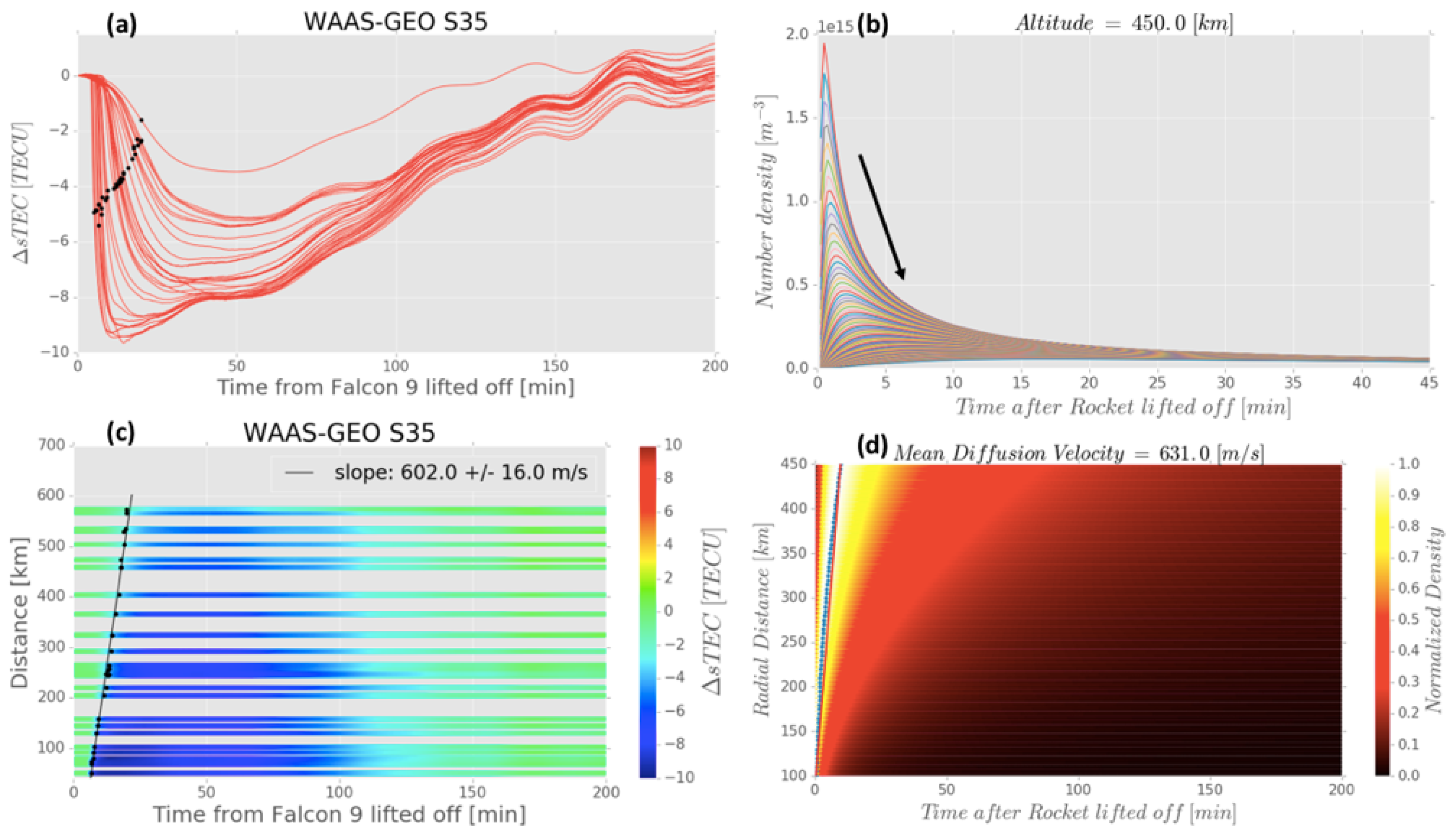
2.5. Diffusion Velocity Simulation

In this section, we briefly describe a diffusion model adapted from [8,29] to quantify how quickly the neutral constituents ($H_2$ and $H_{2}O$) diffuse from the exhaust plume into the weakly ionized plasma medium. The diffusion speed of the neutral molecules strongly controls the development and shape of the hole in spatial and temporal domain. The main elements of the model are:

• The neutral gasses from the plume can be considered to have entered the ionosphere at zero speed.
• The dispersion is considered to be highly governed by diffusion rather than advection.
• The diffusion is considered isotropic at every effusion point.

Due to the trajectory of this rocket (see Figure S7), this model is considered to describe well the diffusion of the neutral gasses contained in the exhaust plume into the ionosphere. Under the previous hypotheses, the total concentration of the depositions at a certain time t and radial distance r from the effusion point can be given by:

$$n(r,t)=\frac{E_0^{H_{2}O}}{{(4\pi D^{H_{2}O}t)}^{3/2}}exp(-\frac{r^2}{4D^{H_{2}O}t})+\frac{E_0^{H_2}}{{(4\pi D^{H_2}t)}^{3/2}}exp(-\frac{r^2}{4D^{H_2}t}),$$

(4)

where $E_0$ is the total number of molecules. We considered the diffusion coefficient (D) at 450 km altitude [2,7] in order to account for the rocket trajectory. Since the $H_2$ diffuses more rapidly than $H_{2}O$, the onset of the TEC depletion is determined by the arrival of the $H_2$ front, while its duration is due mainly to the persistency of $H_{2}O$. Since the time lag between the rocket passage and the hole formation is very small (see simulation results in [7,8]), we ran a simulation to quantify the velocity of expansion of the hole by interpolating the time evolution of the maxima of the total concentration $n(r,t)$ at different locations. These results are presented in the next section.

3. Results

In this study, we processed WAAS-GEO observations from 62 PBO GNSS stations to estimate $\mathsf{\Delta }sTEC$ perturbations caused by the Falcon 9 rocket launch using the VARION algorithm in a simulated real-time scenario. Figure 3 shows the unfiltered VARION-GPS solutions (red curves) for four satellites tracked by the 62 GNSS stations. These unfiltered VARION-GPS $\mathsf{\Delta }sTEC$ solutions show an ionospheric plasma depletion up to about 4 TECU, which is 40% less than the value estimated from the VARION-GEO solutions. This quantitative discrepancy could be partly due to the fact that the GEO and GPS observations were obtained at different elevation and azimuth angles, therefore they are representative of different volumes of the ionosphere. In addition, due to the motion of the IPP (Section 2.3), the unfiltered VARION-GPS solutions experience higher trends at low elevation angles (below 20 degrees), and we cannot easily estimate the ionospheric recovery time [7].

An additional insight concerning the filtering technique is presented in the Supplementary Materials, where we clearly show that it is not possible to apply a Butterworth band-pass filter when there is a sharp discontinuity in the data (e.g., ionospheric hole) without generating a non-physical TEC perturbation. We would like to note, however, that this filtering technique can be used in many cases to study waves in the ionosphere, and was successfully applied for instance by the authors of [30,31,32,33,34]. However, Figure S8 shows the effect of a Butterworth filter to non-periodic signal, such as the ionospheric hole detected in the VARION-GEO $\mathsf{\Delta }sTEC$ solutions. Figure S9 shows the effect on the actual VARION-GPS solutions. Taking all these factors into account, we designed a noise reduction algorithm (Section 2.4) to remove the satellite dependent noise from the VARION-GEO solutions. Figure 4 shows the filtered VARION-GEO solutions for satellite S35, for the day before (left column) and the day of the event (right column). Figure 4c,d represents a zoom in for 10 min before to 60 min after the launch. Figure 4d clearly shows the ionospheric plasma density depletion starting 5 min after the rocket launch (red curves). The comparison with the day before highlights the difference with the undisturbed state (no rocket launch). Figure 4 also shows that we were able to successfully remove the noise from the VARION-GEO $\mathsf{\Delta }sTEC$ solutions without modifying the shape and amplitude of the ionospheric perturbation, therefore without removing/adding any geophysical information from the time series.

The reader can find in the Supplementary Materials two figures equivalent to Figure 2 and Figure 4 obtained for another WAAS-GEO satellite S38 (Figures S5 and S6). These results are consistent with the ones obtained with satellite S35, therefore we decided to include just one satellite in the text.

To compare our filtered VARION-GEO $\mathsf{\Delta }sTEC$ solutions with an independent data source, we analyzed ionosonde data from station PA836 located 5 km from the Vandenberg Airforce Base in California. This ionosonde derived electron density profile are available every 15 min (Section 2.1). We analyzed the time variability of the peak electron density (NmF2) and we performed a correlation analysis with the VARION-GEO $\mathsf{\Delta }sTEC$ solutions.

Figure 5a shows the closest VARION-GEO $\mathsf{\Delta }sTEC$ time series to the ionosonde site, while Figure 5b shows the ionosonde peak electron density (NmF2) extracted for each electron density profile measured by the ionosonde and plotted as a function of time. An electron density depletion in the F2 layer is clearly visible from both datasets. To quantify the agreement between the two curves, we applied a min-max normalization to the two curves to bring all values into the range [0, 1]. This procedure allowed us to study the correlation between the two curves: Figure 5c displays the normalized $\mathsf{\Delta }sTEC$ (red) and NmF2 (blue) curves. We then down-sampled the normalized VARION-GEO solutions in order to have the same sampling rate as the ionosonde data (15 min). Finally, we computed the correlation coefficient between the two curves and we found a value of 0.97. Despite the fact the ionosonde electron density profiles extend up to the F2 peak, and that two measurements are not exactly co-located, the agreement between the two datasets is very good.

Figure S10a shows electron density profiles inferred from ionosonde observations, and the corresponding Figure S10b NmF2 time variability, for 40 h before and 5 h after the launch. The ionospheric hole signature is clearly visible in comparison to the previous day measurements.

This comparison between the VARION-GEO and the ionosonde time series shows that VARION-GEO solutions fully capture the ionospheric depletion induced by the interaction of the rocket’s exhaust plume and the ionospheric plasma. Figure 5a shows the estimation of valuable geophysical information from the VARION-GEO $\mathsf{\Delta }sTEC$ solutions such as the recovery time of the ionospheric hole (176.25 min) and the ionospheric bite-out magnitude (7.75 TECU of $\mathsf{\Delta }sTEC$).

To describe the time and space evolution of the ionospheric plasma hole, we also estimated the propagation speed of the ionospheric plasma depletion. Figure 6a displays the VARION-GEO $\mathsf{\Delta }sTEC$ solutions from satellite S35. We considered 50% of the minimum value in order to estimate the reaction starting time at different locations (black dots). Figure 6b shows the results of the diffusion model simulation at 450 km altitude (Section 2.5). Following the black arrow, the curves are obtained from Model (4) for an increasing distance from the effusion point (from 100 to 600 km, every 5 km). Figure 6c shows the $\mathsf{\Delta }sTEC$ variations for 200 min after the launch at the IPPs vs. distance from the effusion point, for satellite S35 observed from the 36 GNSS permanent stations closest to the effusion point. We assumed that the exhaust plume diffusion is homogeneously isotropic and we included all stations regardless of their azimuthal direction with respect to the effusion point. The slope of the straight line was fitted considering a linear least squares regression for corresponding reaction starting time to represent the mean ionospheric hole expansion speed. We estimated from the VARION-GEO $\mathsf{\Delta }sTEC$ solutions a mean speed of about 602 m/s, considering an isotropic diffusion. This velocity estimated with VARION-GEO solutions is also in agreement with the numerical estimation in [2], which reports an apparent velocity of about 600 m/s. The diffusion speed of the neutral molecules ($H_{2}O$, $H_2$) highly controls the development and shape of the hole in spatial and temporal domain. For this reason, we validated the estimated expansion velocity with the mean diffusion velocity of these neutral gasses in the ionosphere. In Figure 6d, we quantify the mean velocity of expansion of the hole, by interpolating the time evolution of the maxima (blue dots) of the total concentration $n(r,t)$. We obtained a value of 630 m/s, which is consistent with the estimated velocity. The difference between the two values can be attributed to the complex interaction between the gas emitted along the trajectory of the rocket and the ionosphere, and the fact that the diffusion speed is mainly controlled by $H_{2}O$ and $H_2$ diffusion coefficients, which increase by more than one order of magnitude from 250 to 450 km altitude [29]. For this reason, different rocket events can generate ionospheric holes expanding with significantly different velocities. A recent analysis of observations of rocket-induced ionospheric depletion in [35] gave a velocity estimate of around 100 m/s. This value is significantly lower than in our case where the second-stage engine continued burning throughout the 84 to 721 km altitude range (see Figure S7).

After estimating the ionospheric plasma expansion speed, we provided a first demonstration of the potentiality of combining GPS with GEO satellites for ionospheric anomaly detection. The two sets of observations have complementary characteristics. While GEO satellites provides continuous and more stable (both with respect to noise and trend) $\mathsf{\Delta }sTEC$ measurements over a fixed location, GPS satellites provide a better spatial coverage of the ionosphere.

Figure 7 displays a sequence of six maps (every 5 min) in the region around Vandenberg Air Force Base in California. These maps show the VARION-GEO $\mathsf{\Delta }sTEC$ solutions at GEO-IPP locations for satellites S35 and S38 (squared markers), and the VARION-GPS solutions for satellites G02, G05, G06, G12, G25, and G29 (circles markers). The colors represent variations in the $\mathsf{\Delta }sTEC$. The ionospheric hole (blue color) is clearly detected from both GEO satellites 5 min after the rocket launch. The GPS satellites start detecting the ionospheric hole as they move inside the depleted ionospheric region. This figure well illustrates the difference between GEO and GPS solutions. VARION-GEO solutions provide a direct estimation of the time evolution of the ionosphere over a fixed location, while VARION-GPS solutions are also affected by the ionospheric spatial gradients as they move along the IPP trajectory (Section 2.3). The figure shows the potential benefits of GEO satellites as a complementary technique for well-established GPS satellites.

In our analysis, we were clearly able to detect and track the abrupt decrease of the TEC since its very beginning thanks to the observed GEO satellites; however, in contrast to Chou [20], we were not able to highlight any circular SAW. We offer a plausible explanation of our different result in the Supplementary Materials, where we provide an insight about the application of the bandpass Butterworth filter to the actual measurements impacted by the ionospheric plasma depletion. This filter was successfully applied in other cases to study waves in the ionosphere [30,31,32,33,34], but it does not seem appropriate here due to the abrupt decrease of the TEC.

4. Conclusions

In this study, we applied for the first time the VARION algorithm to WAAS-GEO satellites in a simulated real-time scenario, in order to describe the ionospheric response associated with the Falcon 9 rocket launch of 24 August 2017 from Vandenberg Air Force Base in California. We demonstrated that the use of GEO satellites as a complementary technique to GPS provides valuable geophysical information, which allows a better description of the time and space evolution of the ionosphere. We designed a noise reduction algorithm, to reduce the satellite dependent noise of the WAAS GEO L1/L5 TEC solutions to a level comparable with GPS L1/L2 TEC solutions. The current implementation of this technique introduces a 3-min delay into the real-time VARION-GEO solutions. We found observational evidence in the VARION-GEO $\mathsf{\Delta }sTEC$ measurements of an ionospheric plasma hole, which depleted the TEC to a level comparable with nighttime values. The ionospheric plasma hole was induced by the interaction of the rocket’s exhaust plume with the ionospheric plasma through dissociative recombination. The VARION solutions clearly show an ionospheric hole appearing 5 min after the rocket lifted-off. This result is in agreement with the rocket’s trajectory, which reached an altitude of around 390 km after 5 min. In the process, it took almost 3 h for the ionospheric plasma density to relax back to a pre-perturbed state. We compared our results with an independent data source and a high correlation coefficient (0.97) was found between the VARION-GEO results and the ionosonde NmF2 data. We estimated the expansion velocity of the ionospheric hole and we found a speed of about 600 m/s. We validated our estimation by simulating the diffusion of exhaust neutral constituents ($H_2$ and $H_{2}O$) into the ionosphere at 450 km.

Our observations showed that the primary effect in the ionosphere following this Falcon 9 rocket launch was due to an ionospheric hole, which started depleting the ionosphere after about 5 min from the launch, unlike the 14 min reported in [20]. Their study also reported a circular shock acoustic wave near the launch site. Since the rocket arrived in the ionosphere first and because of the duration, magnitude, and expansion speed of the induced ionospheric hole, we conclude that any circular shock acoustic wave near the launch site might not be detected using TEC data.

The application of a real-time algorithm (VARION) to GEO satellites opens a prospect of combined use of GNSS and GEO measurements for real-time natural hazard detection. Furthermore, due to the proximity of the GEO-IPPs to the rocket’s effusion point, the VARION-GEO solutions were able to detect the ionospheric hole 5 min prior to any GPS satellites. Even if this may not always be the case since the observational geometry of GNSS satellites changes according to the time of day, we believe that the VARION-GEO technique provides valuable real-time geophysical information which could be particularly useful to augment and enhance capabilities of well-established GNSS-based ionosphere remote sensing techniques and future GNSS ionospheric-based early warning systems. In particular, the fixed GEO-IPPs increase the reliability of a detection scheme using ionospheric remote sensing observations. Up until this publication, the only essential limitation of VARION-GEO is technological, and it is related to the number of ground stations capable of tracking GEO satellites.

As a future prospect of this research, a time- and space-dependent ionospheric layer height will be implemented in the VARION algorithm.

References

1. Booker, H.G. A local reduction of F-region ionization due to missile transit. J. Geophys. Res. 1961, 66, 1073–1079. [Google Scholar] [CrossRef]
2. Mendillo, M.; Hawkins, G.S.; Klobuchar, J.A. A sudden vanishing of the ionospheric F region due to the launch of Skylab. J. Geophys. Res. 1975, 80, 2217–2225. [Google Scholar] [CrossRef]
3. Bernhardt, P.A.; Huba, J.D.; Kudeki, E.; Woodman, R.F.; Condori, L.; Villanueva, F. Lifetime of a depression in the plasma density over Jicamarca produced by space shuttle exhaust in the ionosphere. Radio Sci. 2001, 36, 1209–1220. [Google Scholar] [CrossRef]
4. Bernhardt, P.A.; Erickson, P.J.; Lind, F.D.; Foster, J.C.; Reinisch, B.W. Artificial disturbances of the ionosphere over the Millstone Hill Incoherent Scatter Radar from dedicated burns of the space shuttle orbital maneuver subsystem engines. J. Geophys. Res. 2005, 110, A05311. [Google Scholar] [CrossRef]
5. Bernhardt, P.A.; Ballenthin, J.O.; Baumgardner, J.L.; Bhatt, A.; Boyd, I.D.; Burt, J.M.; Caton, R.G.; Coster, A.; Erickson, P.J.; Huba, J.D.; et al. Ground and space-based measurement of rocket engine burns in the ionosphere. IEEE Trans. Plasma Sci. 2012, 40, 1267–1286. [Google Scholar] [CrossRef]
6. Mendillo, M.; Smith, S.; Coster, A.; Erickson, P.; Baumgardner, J.; Martinis, C. Man-made space weather. Space Weather 2008, 6, S09001. [Google Scholar] [CrossRef]
7. Furuya, T.; Heki, K. Ionospheric hole behind an ascending rocket observed with a dense GPS array. Earth Planets Space 2008, 60, 235–239. [Google Scholar] [CrossRef] [Green Version]
8. Ozeki, M.; Heki, K. Ionospheric holes made by ballistic missiles from North Korea detected with a Japanese dense GPS array. J. Geophys. Res. 2010, 115, A09314. [Google Scholar] [CrossRef]
9. Nakashima, Y.; Heki, K. Ionospheric hole made by the 2012 North Korean rocket observed with a dense GNSS array in Japan. Radio Sci. 2014, 49, 497–505. [Google Scholar] [CrossRef] [Green Version]
10. Arendt, P.R. Ionospheric undulations following Apollo 14 launching. Nature 1971, 231, 438. [Google Scholar] [CrossRef]
11. Noble, S.T. A large-amplitude traveling ionospheric disturbance excited by the Space Shuttle during launch. J. Geophys. Res. 1990, 95, 19037–19044. [Google Scholar] [CrossRef]
12. Kakinami, Y.; Yamamoto, M.; Chen, C.-H.; Watanabe, S.; Lin, C.; Liu, J.-Y.; Habu, H. Ionospheric disturbances induced by a missile launched from North Korea on 12 December 2012. J. Geophys. Res. Space Phys. 2013, 118, 5184–5189. [Google Scholar] [CrossRef]
13. Ding, F.; Wan, W.; Mao, T.; Wang, M.; Ning, B.; Zhao, B.; Xiong, B. Ionospheric response to the shock and acoustic waves excited by the launch of the Shenzhou 10 spacecraft. Geophys. Res. Lett. 2014, 41, 3351–3358. [Google Scholar] [CrossRef]
14. Mannucci, A.J.; Wilson, B.D.; Yuan, D.N.; Ho, C.H.; Lindqwister, U.J.; Runge, T.F. A global mapping technique for GPS derived ionospheric total electron content measurements. Radio Sci. 1998, 33, 565–582. [Google Scholar] [CrossRef]
15. Komjathy, A.; Sparks, L.; Wilson, B.D.; Mannucci, A.J. Automated daily processing of more than 1000 ground-based GPS receivers for studying intense ionospheric storms. Radio Sci. 2005, 40, RS6006. [Google Scholar] [CrossRef]
16. Sardon, E.; Rius, A.; Zarraoa, N. Estimation of the transmitter and receiver differential biases and the ionospheric total electron content from Global Positioning System observations. Radio Sci. 1994, 29, 577–586. [Google Scholar] [CrossRef]
17. Hajj, G.A.; Lee, L.C.; Pi, X.; Romans, L.J.; Schreiner, W.S.; Straus, P.R.; Wang, C. COSMIC GPS ionospheric sensing and space weather. Terr. Atmos. Ocean. Sci. 2000, 11, 235–272. [Google Scholar] [CrossRef]
18. Savastano, G.; Komjathy, A.; Verkhoglyadova, O.; Mazzoni, A.; Crespi, M.; Wei, Y.; Mannucci, A.J. Real-Time Detection of Tsunami Ionospheric Disturbances with a Stand-Alone GNSS Receiver: A Preliminary Feasibility Demonstration. Sci. Rep. 2017, 7, 46607. [Google Scholar] [CrossRef]
19. Fratarcangeli, F.; Ravanelli, M.; Mazzoni, A.; Colosimo, G.; Benedetti, E.; Branzanti, M.; Savastano, G.; Verkhoglyadova, O.; Komjathy, A.; Crespi, M. The variometric approach to real-time high-frequency geodesy. Rend. Fis. Acc. Lincei 2018, 29, 95. [Google Scholar] [CrossRef]
20. Chou, M.-Y.; Shen, M.-H.; Lin, C.C.H.; Yue, J.; Chen, C.-H.; Liu, J.-Y.; Lin, J.-T. Gigantic circular shock acoustic waves in the ionosphere triggered by the launch of FORMOSAT-5 satellite. Space Weather 2018, 16, 172–184. [Google Scholar] [CrossRef]
21. Huang, F.; Lei, J.; Dou, X. Daytime ionospheric longitudinal gradients seen in the observations from a regional BeiDou GEO receiver network. J. Geophys. Res. Space Phys. 2017, 122, 6552–6561. [Google Scholar] [CrossRef]
22. Yang, H.; Yang, X.; Zhang, Z.; Zhao, K. High-Precision Ionosphere Monitoring Using Continuous Measurements from BDS GEO Satellites. Sensors 2018, 18, 714. [Google Scholar] [CrossRef] [PubMed]
23. Padokhin, A.M.; Tereshin, N.A.; Yasyukevich, Y.V.; Andreeva, E.S.; Nazarenko, M.O.; Yasyukevich, A.S.; Kozlovtseva, E.A.; Kurbatov, G.A. Application of BDS-GEO for studying TEC variability in equatorial ionosphere on different time scales. Adv. Space Res. 2018, 63, 257–269. [Google Scholar] [CrossRef]
24. Cooper, C.; Mitchell, C.N.; Wright, C.J.; Jackson, D.R.; Witvliet, B.A. Measurement of ionospheric total electron content using single-frequency geostationary satellite observations. Radio Sci. 2019, 54, 10–19. [Google Scholar] [CrossRef]
25. Kunitsyn, V.E.; Padokhin, A.M.; Kurbatov, G.A.; Yasyukevich, Y.V.; Morozov, Y.V. Ionospheric TEC estimation with the signals of various geostationary navigational satellites. GPS Solut. 2016, 20, 877. [Google Scholar] [CrossRef]
26. Savastano, G. New Applications and Challenges of GNSS Variometric Approach. Ph.D. Thesis, Department DICEA, Università La Sapienza, Rome, Italy, 2018. Available online: http://hdl.handle.net/11573/1077041 (accessed on 7 May 2019).
27. Chen, Y.-H.; Juang, J.-C.; De Lorenzo, D.S.; Seo, J.; Lo, S.; Enge, P.; Akos, D.M. Real-Time Dual-Frequency (L1/L5) GPS/WAAS Software Receiver. In Proceedings of the 24th International Technical Meeting of The Satellite Division of the Institute of Navigation (ION GNSS 2011), Portland, OR, USA, 19–23 September 2011; pp. 767–774. [Google Scholar]
28. Fratarcangeli, F.; Savastano, G.; D’Achille, M.C.; Mazzoni, A.; Crespi, M.; Riguzzi, F.; Devoti, R.; Pietrantonio, G. VADASE Reliability and Accuracy of Real-Time Displacement Estimation: Application to the Central Italy 2016 Earthquakes. Remote Sens. 2018, 10, 1201. [Google Scholar] [CrossRef]
29. Ssessanga, N.; Kim, Y.H.; Choi, B.; Chung, J.-K. The 4D-var estimation of North Korean rocket exhaust emissions into the ionosphere. J. Geophys. Res. Space Phys. 2018, 123, 2315–2326. [Google Scholar] [CrossRef]
30. Calais, E.; Minster, J.B. GPS detection of ionospheric perturbations following the January 17, 1994, Northridge earthquake. Geophys. Res. Lett. 1995, 22, 1045–1048. [Google Scholar] [CrossRef]
31. Calais, E.; Minster, J.B. GPS detection of ionospheric perturbations following a space shuttle ascent. Geophys. Res. Lett. 1996, 23, 1897–1900. [Google Scholar] [CrossRef]
32. Chen, C.H.; Saito, A.; Lin, C.H.; Liu, J.Y.; Tsai, H.F.; Tsugawa, T.; Otsuka, Y.; Nishioka, M.; Matsumura, M. Long-distance propagation of ionospheric disturbance generated by the 2011 off the Pacific coast of Tohoku Earthquake. Earth Planets Space 2011, 63, 67. [Google Scholar] [CrossRef]
33. Bowling, T.; Calais, E.; Haase, J.S. Detection and modelling of the ionospheric perturbation caused by a space shuttle launch using a network of ground-based Global Positioning System stations. Geophys. J. Int. 2013, 192, 1324–1331. [Google Scholar] [CrossRef]
34. Lin, C.C.; Shen, M.H.; Chou, M.Y.; Chen, C.H.; Yue, J.; Chen, P.C.; Matsumura, M. Concentric traveling ionospheric disturbances triggered by the launch of a SpaceX Falcon 9 rocket. Geophys. Res. Lett. 2017, 44, 7578–7586. [Google Scholar] [CrossRef]
35. Liu, H.; Ding, F.; Yue, X.; Zhao, B.; Song, Q.; Wan, W.; Ning, B.; Zhang, K. Depletion and traveling ionospheric disturbances generated by two launches of China’s Long March 4B rocket. J. Geophys. Res. Space Phys. 2018, 123, 10319–10330. [Google Scholar] [CrossRef]
Figure 1. (left) Map showing the IPPs location for satellites S35 (blue dots) and S38 (yellow dots) seen from the 62 GNSS stations. The IPPs for GEO satellites can be considered to be fixed over time. The red dot represents the location of the ionosonde site PA836. (right) Two maps representing the Earth as seen from WAAS-GEO satellites S35 and S38.
Remotesensing 11 01734 g001
Figure 2. VARION-GEO δ s T E C results for satellite S35. Day before (left column) and day of the event (right column). The first row (a,b) represents the unfiltered VARION-GEO δ s T E C solutions far from the ionospheric hole (distance greater than 700 km). Time zero represents the time of the Falcon 9 launch (11:51 PDT). The second row (c,d) represents the unfiltered VARION-GEO δ s T E C solutions close to the ionospheric hole (distance smaller than 700 km).
Remotesensing 11 01734 g002
Figure 3. Unfiltered VARION-GPS δ s T E C solutions (red curves) for satellites G12, G25, G02, and G05. The blue curves show the elevation angle for each satellite-receiver link. The δ s T E C solutions show a lower high-frequency noise compared to the VARION-GEO solutions (Figure 2). However, the higher long period trends in the unfiltered VARION-GPS solutions do not allow fully capturing the ionospheric response to the rocket launch.
Remotesensing 11 01734 g003
Figure 4. Filtered VARION-GEO Δ s T E C results for satellite S35. Day before (left column) and day of the event (right column). The first row (a,b) represents the solutions far from the ionospheric hole (blue curves) and close to the ionospheric hole (red curves). Time zero represents the time of the Falcon 9 launch (11:51 PDT). The second row (c,d) is a zoom in 10 min before to 60 min after the launch. The ionospheric depletion is clearly captured by the filtered VARION-GEO solutions near the ionospheric hole for the day. No depletion is showed either the day before or far from the hole.
Remotesensing 11 01734 g004
Figure 5. (a) The VARION-GEO Δ s T E C solutions obtained from station p215, satellite S38; (b) the NmF2 time variability obtained from ionosonde PA836; and (c) the down-sampled and normalized Δ s T E C solutions (red curve) and the normalized NmF2 time series (blue curve) plotted using a common scale [0, 1]. This figure shows a high correlation between the VARION-GEO Δ s T E C solutions and ionosonde data. The correlation coefficient between the two curves is 0.97.
Remotesensing 11 01734 g005
Figure 6. (a,c) The filtered VARION-GEO Δ s T E C solutions for satellite S35. The black dots represent 50% of the minimum of Δ s T E C . (c) The Δ s T E C solutions plotted on a time vs. distance plot. We interpolated the black dots to estimate a mean expansion velocity of the ionospheric hole. (b,d) The results of the diffusion simulation at 450 km of altitude. (b) The density time series at a fixed distance from the diffusion point. Following the black arrow, we computed the curves from 100 to 600 km, every 5 km. (d) The time vs. distance plot for the simulation. We computed the mean diffusion velocity of the number density maxima.
Remotesensing 11 01734 g006
Figure 7. Space-time Δ s T E C variations for 30 min after the launch (one frame every 5 min) at the SIPs (same positions of the corresponding IPPs on the map) for the 2 GEO satellites (square symbols) and six GPS satellites (denoted by circles) seen from the 62 GNSS permanent stations. The ionospheric hole is detected from both GEO satellites 5 min after the rocket launch. The coordinates are expressed in geodetic latitude (in degrees North) and longitude (in degrees west).
Remotesensing 11 01734 g007