The Summertime Diurnal Cycle of Precipitation Derived from IMERG


1
Earth Observation Science Group, Department of Physics and Astronomy, University of Leicester, Leicester LE1 7RH, UK
2
National Centre for Earth Observation, University of Leicester, Leicester LE1 7RH, UK
*
Author to whom correspondence should be addressed.
Remote Sens. 2019, 11(15), 1781; https://0-doi-org.brum.beds.ac.uk/10.3390/rs11151781
Submission received: 20 June 2019
/
Revised: 21 July 2019
/
Accepted: 26 July 2019
/
Published: 30 July 2019
(This article belongs to the Special Issue Precipitation and Water Cycle Measurements Using Remote Sensing)
Abstract
:The Integrated Multi-satellitE Retrievals for GPM (IMERG) precipitation product derived from the Global Precipitation Measurement (GPM) constellation offers a unique opportunity of observing the diurnal cycle of precipitation in the latitudinal band N–S at unprecedented and half-hour resolution. The diurnal cycles of occurrence, intensity and accumulation are determined using four years of data at resolution; this study focusses on summertime months when the diurnal cycle shows stronger features. Harmonics are fitted to the diurnal cycle using a non-linear least squares method weighted by random errors. Results suggest that mean-to-peak amplitudes for the diurnal cycles of occurrence and accumulation are greater over land (generally larger than 25% of the diurnal mean), where the diurnal harmonic dominates and peaks at ~16–24 LST, than over ocean (generally smaller than 25%), where the diurnal and semi-diurnal harmonics contribute comparably. Over ocean, the diurnal harmonic peaks at ~0–10 LST (~8–15 LST) over open waters (coastal waters). For intensity, amplitudes of the diurnal and semi-diurnal harmonics are generally comparable everywhere (~15–35%) with the diurnal harmonic peaking at ~20–4 LST (~3–12 LST) over land (ocean), and the semi-diurnal harmonic maximises at ~5–8 LST and 17–20 LST. The diurnal cycle of accumulation is dictated by occurrence as opposed to intensity.
1. Introduction
Characterising precipitation is a key challenge for the research community and is generally important for many aspects related to society (e.g., flooding, agriculture, water availability, etc.). Characteristics such as occurrence, intensity and duration of precipitation are expected to be more strongly influenced by climate change than accumulation, and models are expected to represent such characteristics accurately for better simulations and forecasts [1]. A test of model-representation of precipitation characteristics is how well they capture the diurnal cycle of precipitation, with observations paramount in outlining model deficiencies [1]. In fact, model simulations have been found to precede the observed peak in precipitation by several hours [1,2], and have difficulty in representing the diurnal cycle [1].
Obtaining the necessary spatio-temporal resolution and coverage to accurately observe the diurnal cycle globally is challenging without the use of multiple satellites. Previous observational studies using weather stations [3,4,5] have been restricted by spatial coverage, whilst those using single sun-asynchronous orbit satellites (i.e., the Tropical Rainfall Measuring Mission, TRMM) have been susceptible to sampling issues [6,7,8]. Constellations of satellites offer the obvious advantage of closely repeated observations and coverage over remote regions but require proper cross-calibration between the different sensors. Radars indisputably provide the best precipitation estimates as they directly observe the vertical structure of precipitating systems. However, spaceborne precipitation radars provide limited spatial coverage as typically only one has been in space since 1997 [9,10]. Consequently, satellite constellations must include passive microwave (PMW) and infrared (IR) sensors, of which there are many in space (see a subset in Table 1 of [11]), though they provide measurements (e.g., cloud top temperatures) that are less directly related to precipitation.
The TRMM contellation was the first precipitation-oriented satellite constellation, from which the TRMM Multi-satellite Precipitation Analysis product (TMPA) was generated. TRMM TMPA, a merged PMW-IR product with ground-based land gauge adjustment, provides 50N–S coverage at 0.25 0.25 and 3-hour resolution [12] and is commonly used for assessing the diurnal cycle of precipitation [2,13,14]. The product was calibrated by precipitation products from the TRMM satellite’s precipitation radar and microwave radiometer [12] until October 2014, when the precipitation radar measurements became unsuitable as a consequence of the de-orbiting of the TRMM satellite [9]. The TRMM TMPA product, without radar-radiometer calibration from the TRMM satellite, is expected to be produced until mid-2019 [9]. The TRMM follow-up, the NASA-JAXA Global Precipitation Measurement (GPM) Mission Core Observatory (CO), was launched in February 2014 with the first space-borne dual-frequency precipitation radar (DPR) and the GPM microwave imager (GMI) onboard [10,15,16]. The GPM-CO instruments act as calibrators for the Integrated Multi-satellitE Retrievals for GPM (IMERG) product, another multi-satellite merged PMW-IR precipitation product with gauge input, with unprecedented spatial (0.1 0.1) and temporal (half-hour) resolution for 60N–S coverage [11]. Also, IMERG replaced TMPA as the only radar-radiometer calibrated gridded precipitation product in December 2014 [9]. The GPM-CO offers several improvements over TRMM as a calibrator for the multi-satellite product including: Ka-band (35.5 GHz) measurements accompanying Ku-band (13.6 GHz) measurements, which better constrains the precipitation retrieval; additional microwave imager channels at 165.5 GHz and 183.3 GHz, which aid in detecting light and solid precipitation; and an inclination that is no longer constrained to the tropics (GPM: 65; TRMM: 35) [11].
Previous studies demonstrated that IMERG is a suitable product for monitoring the diurnal cycle of precipitation: IMERG precipitation estimates agree with ground-based radar measurements over the contiguous US for temporal resolutions less than 24 h, though there are regional differences [17], and IMERG captures the diurnal cycle of precipitation better than TRMM TMPA over Africa (a region where in situ observations are sparse) [18]. There are several key diurnal cycle features determined by past analyses: (1) diurnal variations in precipitation tend to be better represented by a 24 h harmonic than a 12 h harmonic [3,14]; (2) occurrence is the dominant contributor over intensity to the diurnal cycle of accumulation [14]; (3) the diurnal cycle over land is much stronger than that over ocean, with summertime mean-to-peak amplitudes over land (ocean) at 30–100% (10–30%) of the daily mean accumulation and peaking from afternoon to evening (midnight to early morning) [2,4,7,14]; (4) the diurnal cycle tends to be stronger in summer than in winter over land and comparable between the seasons over the ocean [4,19].
This study aims to use four years of the version-5 (V05) level-3 IMERG product to improve understanding of the summertime diurnal cycles of precipitation accumulation, intensity and occurrence. Focussing on the summertime diurnal cycle is motivated by the stronger diurnal signals during this season over land [4,19]. IMERG offers a novel opportunity to determine the diurnal cycle of precipitation on the global scale thanks to the finest spatio-temporal resolution precipitation estimates for a global product currently available. So far, no global analysis of the diurnal cycle has been conducted with IMERG, and no assessment of the impact of the precipitation product uncertainties onto the diurnal cycle characterisation has been performed. Ultimately, this study provides quantitative analysis of the diurnal cycle across the globe that will be useful for evaluating and constraining model representation of precipitation and its characteristics.
Section 2 outlines the IMERG data product used for analysis and the methodology for deducing the diurnal cycle of precipitation. Section 3 presents case studies of the summertime diurnal cycle for land and ocean regions, and details the results of the analysis including the amplitude and phase of the global summertime diurnal cycle and their uncertainties at 2 2 resolution using 24 h and 12 h harmonics. Furthermore, Section 3 provides an analysis of the variation in the diurnal cycle across the meteorological seasons. Section 4 discusses the results, and finally Section 5 covers the conclusions of the study.
2. Materials and Methods
2.1. Data
Precipitation estimates from a constellation of space-borne passive microwave radiometers and infrared sensors as well as ground-based rain gauges are incorporated into the IMERG product [11]. The IMERG algorithm is described in detail by [11] and summarised by [15,20,21]; the GPM-CO instruments calibrate all microwave precipitation estimates contributing to IMERG, and these estimates then act as calibrators for the infrared estimates. Sampling limitations for passive microwave sensors onboard low-Earth-orbit satellites are addressed by linearly interpolating microwave precipitation estimates using displacement vectors for the motion of features found in infrared estimates, which come from geostationary satellites; this process is known as morphing [22]. Furthermore, precipitation estimates determined from the infrared estimates [23] are incorporated into microwave-sparse regions via a Kalman filter technique to provide near-global gridded precipitation. This study uses the ‘final run’ product (3B-HHR), which is calibrated to monthly Global Precipitation Climatology Centre (GPCC) gauge estimates.
The level-3 IMERG product is processed by the NASA Precipitation Processing System, and the data files are freely available from [24]. The version-5 (V05) product, released in November 2017, is used in this work. The level-3 data provide gridded precipitation estimates at and half-hourly spatial-temporal resolution [15]. Furthermore, the product includes additional parameters such as the weighting of infrared input to the final precipitation estimate, the probability of liquid precipitation, a quality index and others [25]. For this research, the final precipitation estimate after gauge calibration (precipitationCal) and the corresponding random error (randomError) are used. Random errors are determined using an approach similar to [26]; more information can be found in [11,27].
2.2. Methodology
Four years of IMERG data from June 2014 to May 2018 are used to determine the diurnal cycle of precipitation. At each grid box, histograms of precipitation for each half hour of the day are computed by binning seasonal rain rates from across the four–year period into 101 logarithmically spaced classes. For this analysis, summertime is considered to occur in June-July-August in the Northern Hemisphere and December-January-February in the Southern Hemisphere (although it should be noted that summertime is not well defined in the tropics).
Rainfall occurrence, intensity, and accumulation are computed directly from each rain rate histogram. Occurrence is the ratio of rainfall counts to total (zero and positive rain rate) measurements:
where and are the latitude and longitude of the grid box centre, respectively, t is the time of day, and and are the count and average rain rate for the ith rain rate class, respectively. Note that the IMERG threshold for rainfall is 0.1 mm/h. Accumulation is the mean of all rain rates (including zeros):
Intensity is the mean of all positive rain rates, i.e., it is the accumulation conditioned to positive rain rates (same as Equation (2) but with replacing ). If more than 20% of the rainfall estimates in the histogram for a specific grid box and half hour are classed as “missing” then occurrence, intensity and accumulation are not calculated.
Random errors are calculated for accumulation and intensity (see the term in brackets in Equation (2)). The random error () for each rainfall class () at each grid box and for each half hour is computed as:
where is the random error on the jth rainfall estimate that falls within the ith rain rate class. No random error is calculated for occurrence as there is assumed to be zero error in the count per rain rate class ().
The diurnal cycles of occurrence, intensity and accumulation are determined at each grid box by conducting a harmonic analysis [4,14,17,28]. As the diurnal cycle of precipitation can be affected by sub-daily processes, it may not be fully represented by a 24 h harmonic, and may be influenced by higher–order (h) harmonics. Only the first two harmonics are considered as they explain the majority of the diurnal variation in precipitation [4]. Harmonics are fitted to the half hour estimates of occurrence, intensity and accumulation (see Figure 1 and Figure 2) via a non-linear least squares method weighted by the random errors using the harmonic function defined by:
where t is the time of day, is the mean, and are the diurnal (first/24 h harmonic) and semi-diurnal (second/12 h harmonic) mean-to-peak amplitudes, respectively, and and are the phases of the diurnal and semi-diurnal peaks, respectively. The goodness of fit of the harmonic function to the IMERG estimates is assessed using the correlation coefficient (R) between the values assumed by the fitting function in Equation (4) and the estimates, and the ratio of the variance of the function values to the variance of the estimates (). Errors are determined for each of the fit parameters (, , , , ) from the fitting procedure. All times are converted from UTC to local solar time (LST) using the equation:
where longitude is in unit degrees, and UTC and LST are in unit hours. Times are referred to in LST only henceforth.
The harmonic analysis is not conducted on grid boxes where: (1) latitudes are greater than N/S due to the complexity of estimates over snow- and ice-covered surfaces [11], or (2) a rainfall quantity has not been calculated for more than 20% of the daily half hours (note that criterion 2 is only met for seasons other than summertime). These quality controls ensure that incomplete observations do not affect the results. Such regions are represented by blank pixels in the following global plots. In regions that are too arid or where the harmonic fitting provides a limited representation of the diurnal cycle, no statistically significant conclusions can be drawn for the diurnal cycle. Such regions are identified by the following criteria: (1) the diurnal mean accumulation is <0.275 mm; (2) ; (3) the error on an amplitude or phase parameter of the harmonic function (, , , ) surpasses 50% or 3 h. These regions are highlighted by black dots in Figures 4–6 and 8, and are not commented upon henceforth.
3. Results
The summertime diurnal cycles of precipitation occurrence, intensity and accumulation according to IMERG are analysed globally at resolution across a four-year period. Case studies of the diurnal cycles are investigated first, then results are presented for the diurnal mean and the amplitude and phase of the 24 h and 12 h harmonics. Fitting errors on the summertime amplitudes and phases are then analysed, prior to an investigation into the variations in the diurnal cycle of accumulation across the seasons.
A spatial resolution has been selected in all following results. This is a compromise between coarsening the spatial resolution, which reduces the sampling errors, and keeping the finest resolution in order to capture the regional details of the diurnal cycle. In particular, it has been previously shown that there is improvement in the detection of precipitation occurrences and the random errors of IMERG precipitation estimates when passing from to at half-hour resolution [21] (i.e., the probability of detection increases from 0.63 to 0.69, the false alarm ratio reduces from 0.28 to 0.24, the Heidke skill score increases from 0.61 to 0.63, the normalised mean absolute error reduces from 0.68 to 0.6, and the normalised root mean square error reduces from 1.23 to 1.1). The spatial resolution was also selected by [14] for analysis of the diurnal cycle using the TRMM TMPA, CMORPH (Climate Prediction Center morphing) and PERSIANN (Precipitation Estimation from Remotely Sensed Information using Artificial Neural Networks) products. Due to an expected spatial correlation between precipitation estimates and random errors at within a grid box, random error estimates of accumulation and intensity for a specific half hour and grid box (bracketed term in Equation (2)) are increased by a factor of 5 to account for an estimated correlation length of . This estimated correlation length is compatible with passive microwave sensor footprints.
Note that references to morning, afternoon and evening refer to 0–12 LST, 12–18 LST, and 18–24 LST, respectively.
3.1. Case Studies of the Diurnal Cycle of Precipitation
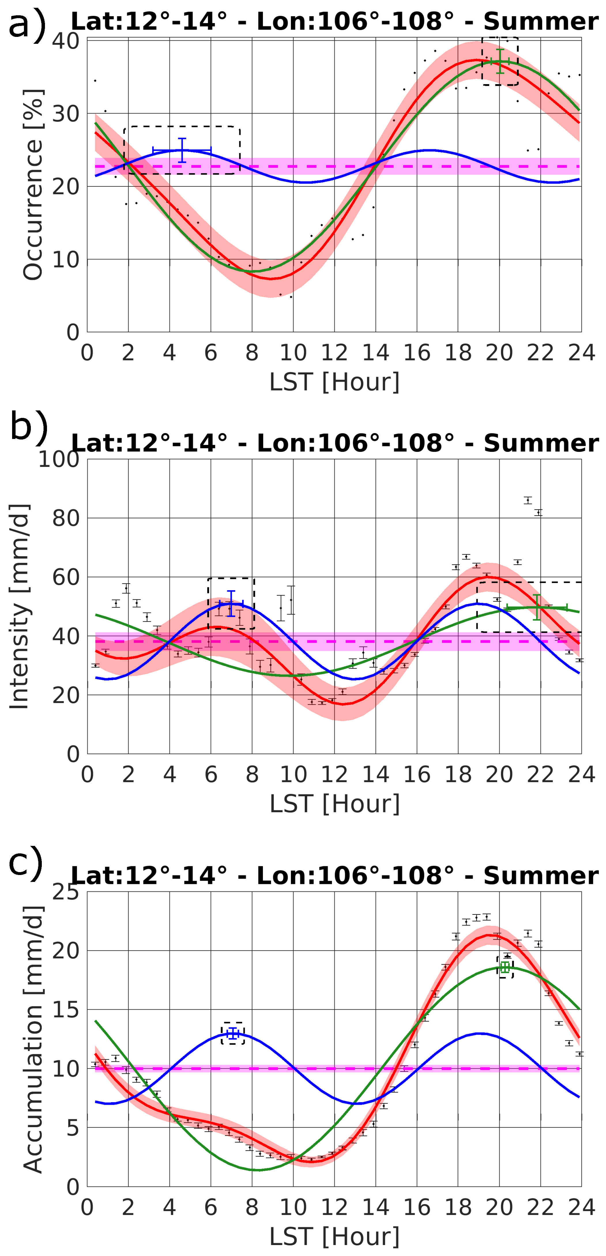
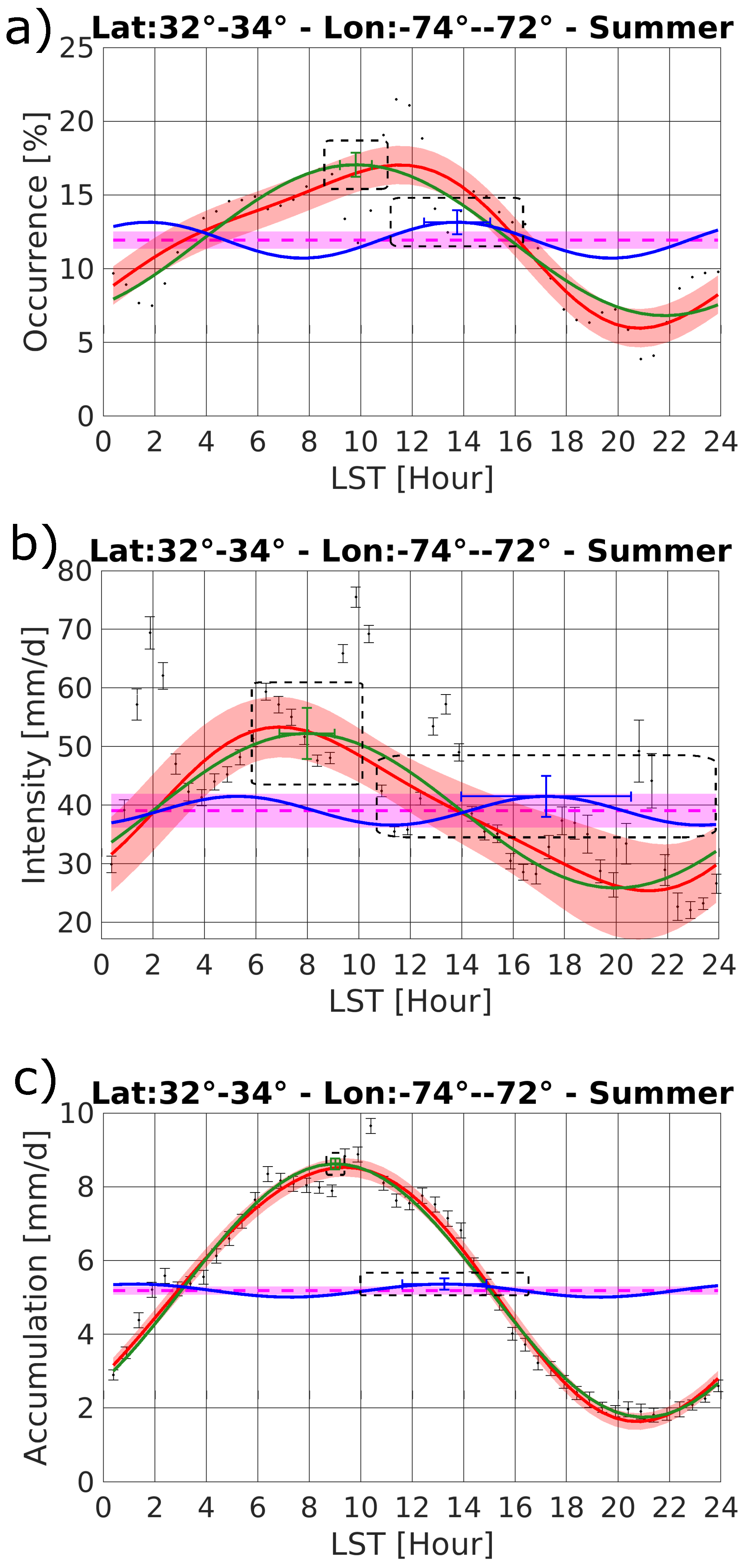
Two case studies are presented to show how the harmonic function is fitted to the IMERG-derived precipitation occurrence, intensity and accumulation. A land-based region over Cambodia and Vietnam, and an oceanic region adjacent to the eastern coast of the US (specifically the states of North and South Carolina) are selected due to their tendency to experience rainfall with a noticeable diurnal variation.
Figure 1 depicts the summertime diurnal cycle of precipitation occurrence, intensity and accumulation for Cambodia and Vietnam. Occurrence and accumulation are clearly dominated by the 24h harmonic (green line), which has a larger amplitude ( 63.4% ± 7.2% and 85.9% ± 4.4%, respectively) in comparison with the 12 h harmonic (blue line, 9.8% ± 7.2% and 29.9% ± 4.5%, respectively). Both occurrence and accumulation peak in the evening, with 20.0 LST ± 0.4 LST and 20.3 LST ± 0.2 LST, respectively. Intensity appears to be evenly contributed to by the 24 h and 12 h harmonics ( 30.4% ± 11.1%, 33.6% ± 11.2%), with the 24 h trough and first 12 h peak superimposing to produce an initial muted diurnal peak at ~6 LST, whilst the 24 h peak and second 12 h peak superimpose to produce a larger second diurnal peak at ~19 LST. The harmonic function appears to better represent precipitation accumulation (, 89.9%) compared to occurrence and intensity ( 0.88 and 0.73, 88.3% and 64.1%, respectively), as evidenced by the smaller deviations in data (black circles) from the harmonic function (red line) and the smaller 95% confidence intervals on the function (red shading). This trend is true for most of the globe, with the harmonic function better fitting to accumulation than to occurrence and intensity (i.e., highest ) for 81.4% of land and ocean quality-controlled grid boxes.
Figure 2 depicts the summertime diurnal cycle of precipitation occurrence, intensity and accumulation for the Atlantic Ocean near the coast of North and South Carolina, US. Occurrence, intensity and accumulation are all dominated by the 24 h harmonic ( 42.8% ± 6.9%, 33.7% ± 11.2% and 66.3% ± 2.9%, respectively) as opposed to the 12h harmonic ( 10.2% ± 6.9%, 6.3% ± 9.0% and 3.4% ± 2.9%, respectively), with the diurnal cycle peaking in the morning at ~12 LST, 7 LST and 10 LST, respectively. As for the land-based case study, the harmonic function best represents accumulation, followed by occurrence and worst represents intensity ( 0.98, 0.79 and 0.52, 97.3%, 79.5% and 52.0%, respectively). Notably for both land and ocean case studies, the amplitude and phase of the 24 h and 12 h harmonics representing the diurnal cycle of intensity should be treated with caution due to the poor fitting of the harmonic function. Clearly the use of only 24 h and 12 h harmonics is not sufficient for capturing the diurnal cycle.
3.2. IMERG Summertime Climatology
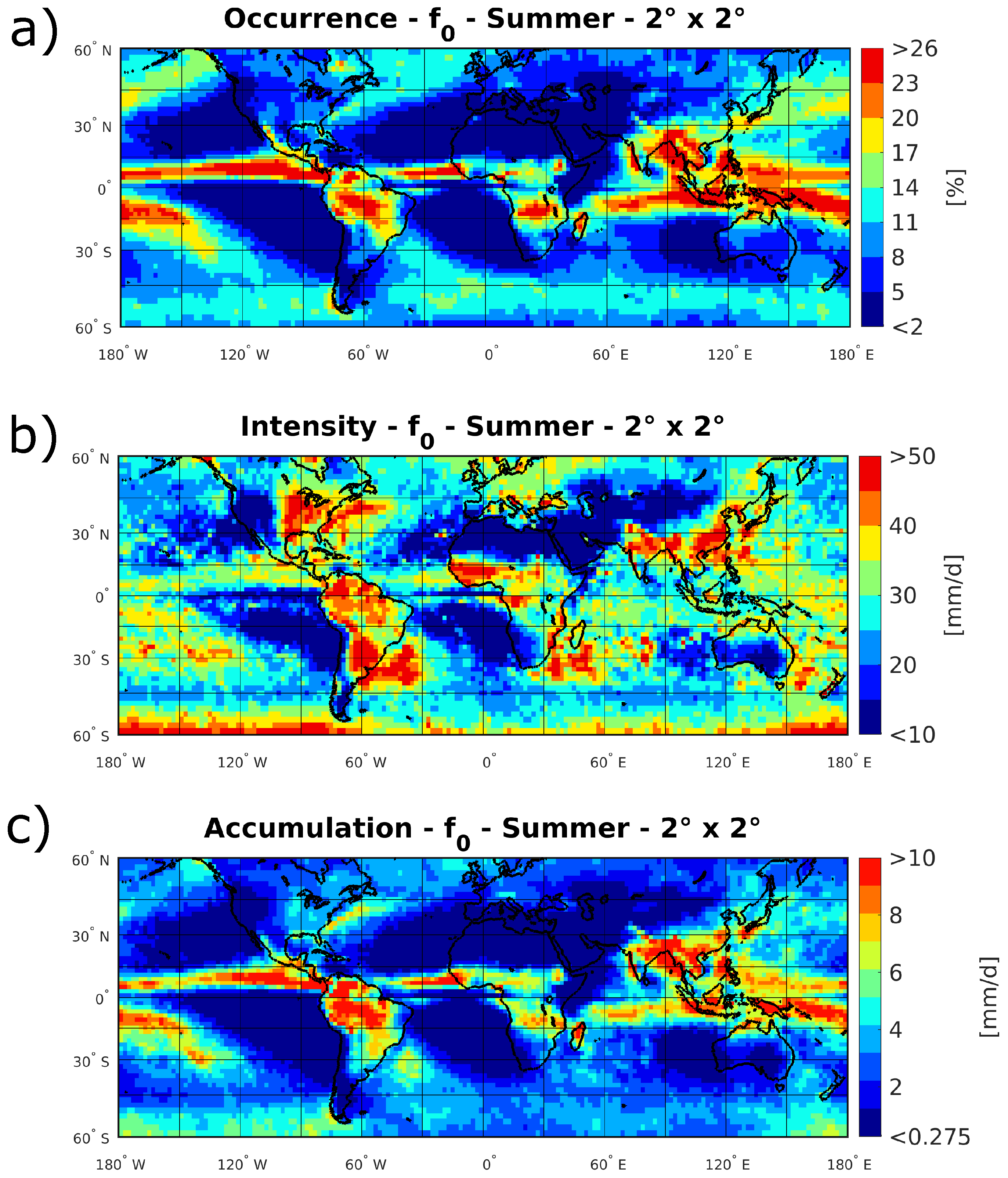
Figure 3 exhibits the summertime diurnal mean precipitation (term in Equation (4)). As previously noticed, the diurnal mean of occurrence, intensity and accumulation is generally highest in the tropics in correspondence with the Intertropical Convergence Zone (ITCZ), especially over land. Either side of the ITCZ, arid regions (where diurnal mean accumulation is less than 0.275 mm) are ever-present in the Sahara and oceans adjacent to the west coasts of Southern Africa and South America. Outside of the tropics, occurrences over the ocean exceed those over land with a sharp increase at higher latitudes (45–60N/S). Conversely, the most intense rainfall is mostly found over land with solar heating and the consequent land-based convection being the dominant driver of precipitation intensity. The most intense regions outside of the tropics tend to be found in Eastern US, South Asia, South America, South-East Africa, and their eastward adjacent coastal oceans. Unexpected precipitation trends are found in the southern oceans in the –S region with diurnal mean occurrence, intensity and accumulation significantly higher for the Pacific Ocean than for the Indian and Atlantic Oceans. The global pattern of diurnal mean accumulation is clearly correlated strongly with occurrence (correlation = 0.94), which highlights that occurrence (and not intensity) is the dominant contributor to accumulation.
3.3. The Amplitude and Phase of the Summertime Diurnal Cycle
The amplitude and phase of the 24 h and 12 h harmonics are shown in Figure 4, Figure 5 and Figure 6. It is considered henceforth that a 30% harmonic amplitude represents a pronounced diurnal cycle [14].
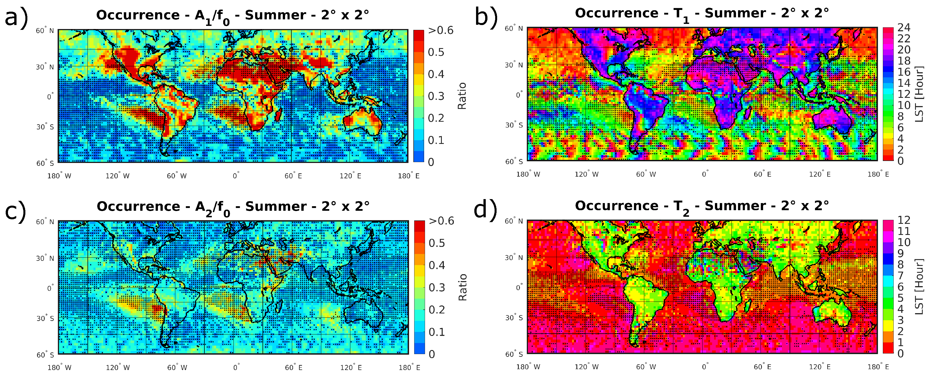
The diurnal cycle of occurrence is mostly dominated by the 24 h harmonic over land, especially in the N–S region with most amplitudes exceeding 25%. Within this region, a pronounced 24 h amplitude is found in areas such as the US and South America, Southern/Eastern Africa, South-East and East Asia, and Northern Australia with 24 h amplitudes exceeding 60%. The 24 h harmonic tends to maximise over land across the evening (~16–24 LST). A pronounced 24 h amplitude is also found over the ocean adjacent to the west of the US and Western Europe. The 12 h amplitude is only comparable with the 24 h amplitude for some oceanic regions where results are reliable (i.e., adjacent to the west coasts of the US, South America, Southern Africa, and Australia), with the harmonic amplitudes unreliable over most of the ocean (see the distribution of black dots). The 24 h maximum occurs in the morning (~3–9 LST) in the oceanic regions where the 24 h and 12 h harmonics are comparable, whilst the maximum occurs earlier in the morning (~0–4 LST) north of 30N. The 12 h maxima occur at 23–2 LST and 11–14 LST over the ocean.
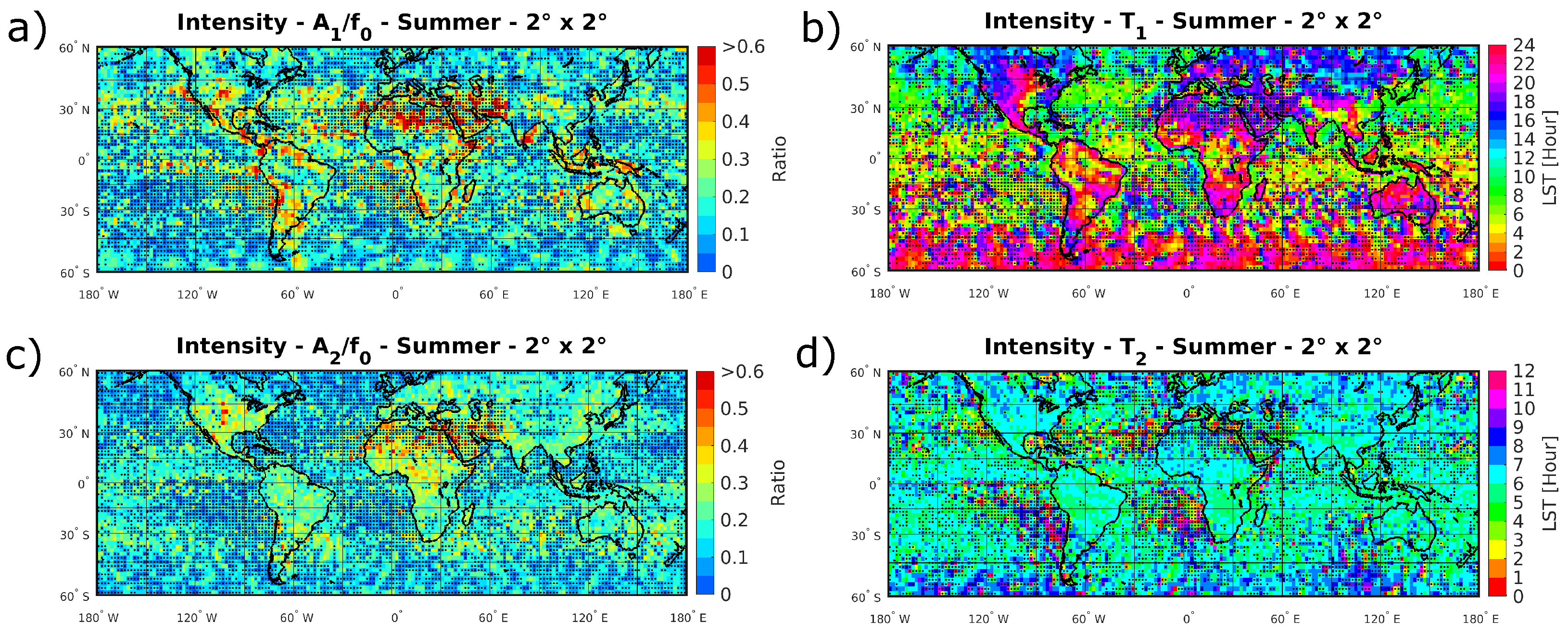
For intensity, the amplitudes of the 24 h and 12 h harmonics are comparable (~15–35%) over land and ocean, with the 12 h harmonic generally slightly stronger over land except for specific regions with quite pronounced 24 h amplitude enhancement (e.g., central US, South American coasts, African coasts, Australia, East and South-East Asia). The 24 h harmonic typically reaches its maximum between evening and early morning over land (~20–4 LST), apart from above 45N where it maximises in the afternoon (~14–18 LST) and in Eastern Asia where it peaks later in the morning (~4–9 LST). Over ocean, the 24 h harmonic tends to maximise in the early to late morning (~3–12 LST), apart from in the 45–60S region where the peak is between late evening and early morning (~20–2 LST). The 12 h harmonic reaches its peak everywhere in the mid morning and the early evening (~5–8 LST and 17–20 LST).
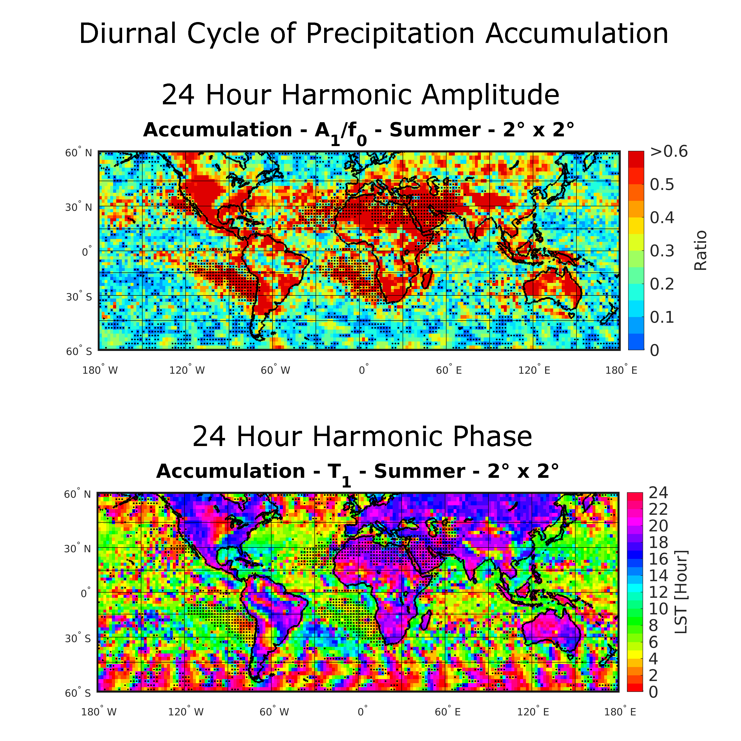
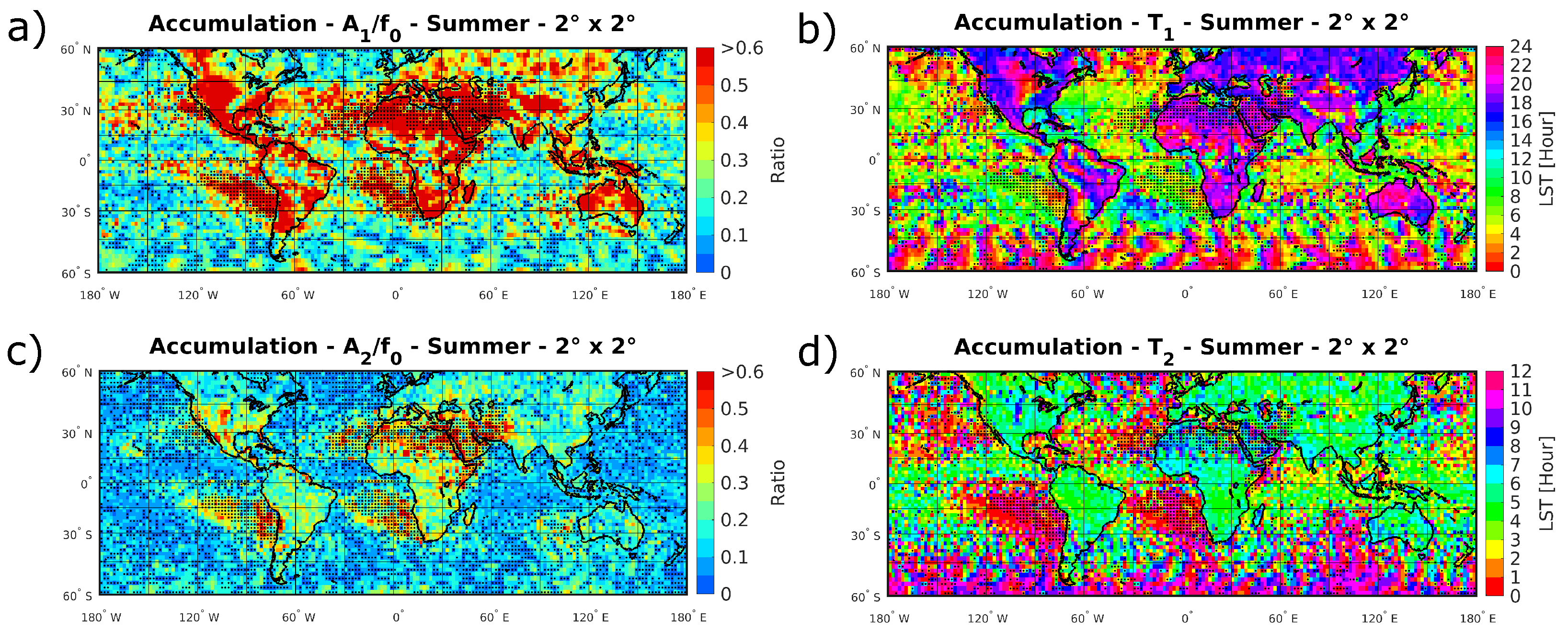
The diurnal cycle of accumulation is dominated by the 24 h harmonic over land with prominent amplitudes in most regions (mostly > 25% and > 60% in many regions), whilst the 24 h harmonic still tends to dominate over ocean but with lesser amplitudes (mostly < 25%). Large diurnal means in the north of South America and in South-East Asia (Figure 3c) combined with large 24 h harmonic amplitudes suggest that there are significant swings in daily accumulation there. 24 h amplitudes over land tend to peak across late afternoon and evening (~16–24 LST), whilst amplitudes over the ocean tend to reach their maximum in the morning (~4–10 LST) with phases typically into the early afternoon (late evening and early morning) in the coastal regions (45–60N/S). The 12 h harmonic typically peaks in mid morning and between late afternoon and early evening (~4–8 LST and 16–20 LST) over land and the oceanic convergence zones (ITCZ, South Pacific Convergence Zone/SPCZ), whilst it reaches its maximum around late evening and late morning (~21–1 LST and 9–13 LST) in the rest of the ocean.
Notably, intensity exhibits more black-dotted regions than accumulation, which suggests that the harmonic function better represents the diurnal cycle of accumulation over most regions.
3.4. Fitting Errors on the Amplitude and Phase of the Summertime Diurnal Cycle
Fitting errors on the diurnal cycle of accumulation are shown in Figure 7. For this analysis, harmonic amplitudes or phases with errors that exceed 50% or 3 h are considered unreliable. Errors are found to be small over land; typically they are less than 15% (25%) for the amplitude and less than 0.75 h (0.75 h) for the 24 h (12 h) harmonic. Over ocean, errors in the amplitude and phase of the harmonics are typically higher, especially in the coastal and 45–60N/S regions. In fact, 24 h amplitudes are mostly found to be unreliable in the 45–60N/S oceanic regions, whilst 12 h amplitudes are found to be mostly unreliable over the ocean. Overall, harmonic parameters for land are mostly reliable, whilst phases are mostly reliable over ocean in the 45N–45S region and amplitudes are generally unreliable over the ocean.
With regards to the fitting errors for precipitation occurrence and intensity (not shown), the distribution of unreliable amplitudes and phases is generally worse than for accumulation. For occurrence, reliable 24 h amplitudes and phases are found over land and north of 30N over ocean, whilst 12 h amplitudes (phases) are generally unreliable (reliable) globally. For intensity, the 24 h amplitudes are unreliable almost everywhere (apart from patches of land), whilst the 24 h phases are unreliable for patches across most of the globe (though less so over land). The 12 h amplitudes are unreliable over ocean and patches of land, and the 12 h phases are reliable almost everywhere apart from some coastal regions of the ocean.
3.5. Variations in the Diurnal Cycle of Accumulation across the Seasons
The amplitude and phase of the 24 h harmonic representing the diurnal cycle of accumulation for each meteorological season are shown in Figure 8. Considering seasonal variations in the diurnal cycle is particularly important in the tropics, where summertime is not well defined.
Over land, seasonal variations in diurnal amplitude are generally larger in the mid-latitudes than the tropics. The tropics tend to have strong amplitudes across all seasons, with some seasonal trends in the north of South America and central Africa. Over the ocean, diurnal amplitudes tend to be weaker across all seasons, though strong diurnal variations are found across the North Atlantic Ocean. In general, summertime diurnal amplitudes in the mid-latitudes generally exceed those in the wintertime.
The time of maximum diurnal accumulation tends to show little seasonal variation. Accumulation generally peaks in the late afternoon and evening over land across all seasons, however some morning and early afternoon peaks can be found in the northern mid-latitudes and Australia outside of the summer season. Over the ocean, accumulation peak times are quite noisy across the seasons, however accumulation generally peaks in the early to mid morning in the tropics. Times of maximum accumulation in the mid-latitude oceans are generally noisiest in wintertime.
4. Discussion
Aspects of agreement and disagreement with previous studies [2,3,4,14] are highlighted, as well as novelties of this study.
- As previously suggested [3,4,14], the diurnal cycles of occurrence and accumulation are largely captured by the 24 h harmonic over land, though the 12 h harmonic is comparable in contribution with the 24 h harmonic over the ocean (Figure 4a,c and Figure 6a,c). A novelty of this study is that the 24 h and 12 h amplitudes for intensity are found to contribute comparably over most regions, with the superposition of the two harmonics leading to enhanced and muted peaks in the diurnal cycle (e.g., Figure 1b,c).
- As previously found [14], occurrence is clearly the main driver of the diurnal cycle of accumulation, as opposed to intensity. This is supported in this study by a strong correlation between occurrence and accumulation (Figure 3a,c), as well as coincidence of the regions where the 24 h amplitudes are pronounced (Figure 4a and Figure 6a) and similar phases of the 24 h harmonic peaks (Figure 4c and Figure 6c) corroborate this strong relationship.
- The 24 h harmonic is the main contributor to the diurnal cycle of accumulation with large amplitudes (mostly > 25%) over land, peaking in the late afternoon and evening (Figure 6). Furthermore, 24 h amplitudes over ocean are again shown to be smaller (mostly < 25%) with mostly morning peaks as previously found [2,14], though some early afternoon peaks in the coastal regions should be noted.
- Large disagreements between the peak time of the 12 h harmonic for accumulation north of 30 have been identified between IMERG and a selection of other satellite precipitation products (TRMM TMPA, CMORPH, PERSIANN). Whilst TRMM TMPA and PERSIANN tend to maximise at ~3–7 LST and 15–19 LST and CMORPH tends to maximise at ~5–8 LST and 17–20 LST (see Figure 6 of [14]), IMERG tends to maximise at ~21–1 LST and 9–13 LST (Figure 6d). Errors on the IMERG phases exceeding 1 h can be found in such regions and may explain some of the discrepancies.
- When comparing the diurnal harmonic of accumulation between IMERG and TRMM TMPA, it is clear that the IMERG amplitude is much larger (~30–60%, Figure 6a) than the corresponding TRMM amplitude (~20–40%, see Figure 5j of [14]) over the North Atlantic and Pacific Oceans. Small errors in the IMERG amplitudes in these regions do not appear to explain such differences.
The results determined from the 4-year period are unaffected by sampling issues or the strong El Nino event of 2015–2016. Comparison of the results with those deduced using the same methodology but with a 2-year period (excluding 2015–2016, not shown) are found to be nearly indiscernible, which highlights that El Nino events do not strongly impact the diurnal cycle of precipitation though there are perceptible differences in accumulations. Furthermore, it suggests that a 4-year period is sufficient for analysing the diurnal cycle. Future studies could investigate the impact of El Nino onto the regional diurnal cycle.
This study only accounts for random errors of IMERG precipitation estimates when deducing the diurnal cycle of precipitation (accumulation and intensity only). Whilst systematic errors in the IMERG precipitation estimates could be taken into consideration, IMERG only slightly underestimates precipitation at resolution (the version-3 IMERG product has a normalised mean error of ~−0.06 [21]). A future IMERG validation study could assess the systematic bias in the IMERG product as a function of rainfall accumulation and intensity, however it is expected that such systematic errors are unlikely to drastically affect the amplitude and phase of the diurnal cycle estimated in this study.
Future research should aim to better account for the correlation length of precipitation estimates when averaging spatially. In particular, deduction of correlation lengths for different precipitation types, latitudes and land types are recommended. Other future work could address the physical reasoning for why the harmonic function (Equation (4)) better fits to the diurnal cycle of accumulation as opposed to the diurnal cycles of occurrence and intensity.
Finally, a note of caution is raised for the interpretation of the results in the 45–60S region where high mean precipitation accumulations, intensities and occurrences are found in the Pacific Ocean compared to the Indian and Atlantic Oceans. These features are not found in other multi-satellite products [14] with mean accumulations up to ∼80% larger in IMERG than for other precipitation products such as DPR, CORRA (DPR & GMI combined), GPROF (multi-satellite PMW product), etc. [15]. The cause of these artifacts is currently under investigation.
5. Conclusions
This study has analysed the summertime diurnal cycles of precipitation occurrence, intensity and accumulation globally at resolution using four years of IMERG final run version-5 data for the period June 2014 to May 2018. A harmonic analysis was conducted on the data and their uncertainties to extract the diurnal (24 h) and semi-diurnal (12 h) harmonics from the diurnal cycle, and to quantify their amplitudes, phases and respective errors. The results of the analysis can be summarised as follows:
- The diurnal cycles of occurrence and accumulation over land are mainly contributed to by the 24 h harmonic, which tends to peak across late afternoon and evening (~16–24 LST), compared to the 12 h harmonic, which tends to peak in the early to mid morning and early afternoon to early evening (~2–8 LST and 14–20 LST) (Figure 4 and Figure 6). However over ocean, the contributions are comparable for the 12 h harmonic, which tends to peak between late evening to early morning and late morning to early afternoon outside of the convergence zones (~21–2 LST and 9–14 LST), and the 24 h harmonic, which peaks in the morning in open regions (~0–10 LST) and between late morning and afternoon in the coastal regions (~8–15 LST). The diurnal cycle of intensity is similarly contributed to by the 24 h harmonic, which typically peaks between mid evening and early morning (~20–4 LST) over land ( N–S) and early to late morning (~3–12 LST) over ocean, and the 12 h harmonic, which peaks in the mid morning and the early evening (~5–8 LST and 17–20 LST) everywhere (Figure 5).
- The diurnal cycle of occurrence dictates the diurnal cycle of accumulation as opposed to intensity. This is supported by strong correlations in diurnal means between occurrence and accumulation (Figure 3a,c), in increased amplitudes in the 24 h harmonic regions (Figure 4a and Figure 6a), and in the time at which the 24 h harmonic peaks (Figure 4c and Figure 6c).
- Fitting errors on the 24 h and 12 h harmonics representing the diurnal cycle suggest that results over land are generally more reliable than over ocean, phases are generally more reliable than amplitudes, and that results for accumulation are generally more reliable than for occurrence and intensity (Figure 7). In particular, amplitudes and phases for occurrence and intensity should be treated with caution (except for the 24 h harmonic for occurrence over land). Furthermore, amplitudes and phases for accumulation in the 45–60N/S region should be treated with caution.
- The use of 24 h and 12 h harmonics is not sufficient to capture the diurnal cycle of intensity (see the distribution of black dots in Figure 5). Low correlations between the harmonic function and the diurnal cycle derived from IMERG data and/or high error estimates for most of the globe suggest that higher-order harmonics are required to better capture the diurnal cycle of intensity.
- IMERG precipitation estimates in the –S region present some anomalies, and results from these regions should be treated cautiously. This is specifically marked by pronounced precipitation occurrences, intensities and accumulations in this zonal region of the Pacific Ocean compared to the Indian and Atlantic Oceans (Figure 3). These artifacts are under investigation.
- Variations in the diurnal cycle of accumulation across the seasons are minimal in the tropics, where diurnal amplitudes are stronger (mostly exceeding 60% over land) throughout the seasons, and more evident in the mid-latitudes (Figure 8). Summertime mid-latitude diurnal amplitudes tend to exceed those in winter. The diurnal cycle of accumulation tends to maximise at similar times across all seasons over land, whilst more variations are found over the mid-latitude oceans.
- The summertime diurnal cycle of precipitation was unaffected by the strong El Nino event of 2015/2016. This suggests that four years of IMERG data are sufficient for analysing the diurnal cycle of precipitation at resolution.
Improvements in the random errors for the IMERG precipitation estimates are necessary, and are under investigation by the IMERG community [11].
The current constellation of passive microwave radiometers provides unprecedented revisit time (see Figure 4 in [10]); it is paramount to maintain (if not to improve) such microwave constellation in order to curb (reduce) uncertainties in the precipitation-feature morphing procedure between different sampling times.
A future study could focus on identifying the optimum spatial resolution at which the diurnal cycle should be analysed, by statistically assessing the relative importance of the improvements in IMERG precipitation representation and errors with coarser spatio-temporal resolutions [21] against the capture of the localised features of the diurnal cycle at finer spatial resolutions.
The results within this article could provide a variety of opportunities for improving understanding of the diurnal cycle of precipitation. One such opportunity is to use the results for validating models which simulate precipitation and its characteristics; note that the grid box size should be kept consistent for a comparison as the errors in the diurnal cycle may be sensitive to such parameter. Another opportunity is to use these results to identify regions for conducting further analyses of the diurnal cycle. Use of three-dimensional measurements from the GPM dual-frequency precipitation radar in localised studies can aid in better characterising the differences between the diurnal cycles of accumulation, occurrence and intensity. Finally, these results offer the opportunity to optimise the orbit selection for satellites with instruments that are detrimentally affected by precipitation [28].
Author Contributions
Conceptualization, A.B.; methodology, A.B. & D.W.; software, D.W.; validation, D.W. & A.B.; formal analysis, D.W.; investigation, D.W.; resources, D.W. & A.B.; data curation, D.W.; writing—original draft preparation, D.W.; writing—review and editing, A.B. & D.W.; visualization, D.W. & A.B.; supervision, A.B.; project administration, A.B. & D.W.; funding acquisition, D.W. & A.B.
Funding
Daniel Watters was funded by a Natural Environment Research Council studentship awarded through the Central England NERC Training Alliance (CENTA; grant reference NE/L002493/1) and by the University of Leicester. The work by A. Battaglia was funded by ESA in the frame of the RAINCAST project (ESA Contract No. 4000125959/18/NL/NA).
Acknowledgments
The version-5 level-3 IMERG data were provided by the NASA/Goddard Space Flight Center and PPS, which develop and compute the V05 level–3 IMERG data as a contribution to GPM, and archived at the NASA GES DISC. This research used the SPECTRE High Performance Computing Facility at the University of Leicester. The authors thank three anonymous reviewers for their helpful comments and recommendations which greatly helped to improve the manuscript. The authors thank Ranvir Dhillon for providing comments on the manuscript prior to submission.
Conflicts of Interest
The authors declare no conflict of interest. The funders had no role in the design of the study; in the collection, analyses, or interpretation of data; in the writing of the manuscript, or in the decision to publish the results.
Abbreviations
The following abbreviations are used in this manuscript:
| CMORPH | Climate Prediction Center morphing |
| CORRA | Combined Radar-Radiometer |
| DPR | Dual-frequency Precipitation Radar |
| GMI | GPM Microwave Imager |
| GPM-CO | Global Precipitation Measurement Mission Core Observatory |
| GPROF | Goddard Profiling Algorithm |
| IMERG | Integrated Multi-satellitE Retrievals for GPM |
| ITCZ | Intertropical Convergence Zone |
| JAXA | Japan Aerospace Exploration Agency |
| LST | Local Solar Time |
| NASA | National Aeronautics and Space Administration |
| PERSIANN | Precipitation Estimation from Remotely Sensed Information using Artificial Neural Networks |
| PMW | Passive Microwave |
| SPCZ | South Pacific Convergence Zone |
| TMPA | Tropical Rainfall Measuring Mission Multi-satellite Precipitation Analysis |
| TRMM | Tropical Rainfall Measuring Mission |
| US | United States |
| UTC | Coordinated Universal Time |
References
- Trenberth, K.E.; Dai, A.; Rasmussen, R.M.; Parsons, D.B. The changing character of precipitation. Bull. Am. Meteorol. Soc. 2003, 84, 1205–1218. [Google Scholar] [CrossRef]
- Covey, C.; Gleckler, P.J.; Doutriaux, C.; Williams, D.N.; Dai, A.; Fasullo, J.; Trenberth, K.; Berg, A. Metrics for the diurnal cycle of precipitation: Toward routine benchmarks for climate models. J. Clim. 2016, 29, 4461–4471. [Google Scholar] [CrossRef]
- Wallace, J.M. Diurnal variations in precipitation and thunderstorm frequency over the conterminous United States. Mon. Weather Rev. 1975, 103, 406–419. [Google Scholar] [CrossRef]
- Dai, A. Global precipitation and thunderstorm frequencies. Part II: Diurnal variations. J. Clim. 2001, 14, 1112–1128. [Google Scholar] [CrossRef]
- Xiao, C.; Yuan, W.; Yu, R. Diurnal cycle of rainfall in amount, frequency, intensity, duration, and the seasonality over the UK. Int. J. Climatol. 2018, 38, 4967–4978. [Google Scholar] [CrossRef]
- Negri, A.J.; Bell, T.L.; Xu, L. Sampling of the diurnal cycle of precipitation using TRMM. J. Atmos. Ocean. Technol. 2002, 19, 1333–1344. [Google Scholar] [CrossRef]
- Nesbitt, S.W.; Zipser, E.J. The diurnal cycle of rainfall and convective intensity according to three years of TRMM measurements. J. Clim. 2003, 16, 1456–1475. [Google Scholar] [CrossRef]
- Liu, C.; Zipser, E.J. Diurnal cycles of precipitation, clouds, and lightning in the tropics from 9 years of TRMM observations. Geophys. Res. Lett. 2008, 35, L04819. [Google Scholar] [CrossRef]
- Huffman, G.J. The Transition in Multi-Satellite Products from TRMM to GPM (TMPA to IMERG). Technical Report. NASA. 2018. Available online: https://pmm.nasa.gov/sites/default/files/document_files/TMPA-to-IMERG_transition_180827.pdf (accessed on 3 June 2019).
- Hou, A.Y.; Kakar, R.K.; Neeck, S.; Azarbarzin, A.A.; Kummerow, C.D.; Kojima, M.; Oki, R.; Nakamura, K.; Iguchi, T. The Global Precipitation Measurement Mission. Bull. Am. Meteorol. Soc. 2014, 95, 701–722. [Google Scholar] [CrossRef]
- Huffman, G.J.; Bolvin, D.T.; Braithwaite, D.; Hsu, K.; Joyce, R.; Kidd, C.; Nelkin, E.J.; Sorooshian, S.; Tan, J.; Xie, P. NASA Global Precipitation Measurement (GPM) Integrated Multi-SatellitE Retrievals for GPM (IMERG). Algorithm Theoretical Basis Document, Version 5.2; 2018; p. 35. Available online: https://pmm.nasa.gov/sites/default/files/document_files/IMERG_ATBD_V5.2_0.pdf (accessed on 18 June 2019).
- Huffman, G.J.; Bolvin, D.T.; Nelkin, E.J.; Wolff, D.B.; Adler, R.F.; Gu, G.; Hong, Y.; Bowman, K.P.; Stocker, E.F. The TRMM Multisatellite Precipitation Analysis (TMPA): Quasi-Global, Multiyear, Combined-Sensor Precipitation Estimates at Fine Scales. J. Hydrometeorol. 2007, 8, 38–55. [Google Scholar] [CrossRef]
- Bowman, K.P.; Fowler, M.D. The diurnal cycle of precipitation in tropical cyclones. J. Clim. 2015, 28, 5325–5334. [Google Scholar] [CrossRef]
- Dai, A.; Lin, X.; Hsu, K.L. The frequency, intensity, and diurnal cycle of precipitation in surface and satellite observations over low-and mid-latitudes. Clim. Dyn. 2007, 29, 727–744. [Google Scholar] [CrossRef]
- Skofronick-Jackson, G.; Petersen, W.A.; Berg, W.; Kidd, C.; Stocker, E.F.; Kirschbaum, D.B.; Kakar, R.; Braun, S.A.; Huffman, G.J.; Iguchi, T.; et al. The Global Precipitation Measurement (GPM) Mission for Science and Society. Bull. Am. Meteorol. Soc. 2017, 98, 1679–1695. [Google Scholar] [CrossRef]
- Skofronick-Jackson, G.; Kirschbaum, D.; Petersen, W.; Huffman, G.; Kidd, C.; Stocker, E.; Kakar, R. The Global Precipitation Measurement (GPM) mission’s scientific achievements and societal contributions: Reviewing four years of advanced rain and snow observations. Q. J. R. Meteorol. Soc. 2018, 144, 27–48. [Google Scholar] [CrossRef] [PubMed]
- Sungmin, O.; Kirstetter, P. Evaluation of diurnal variation of GPM IMERG-derived summer precipitation over the contiguous US using MRMS data. Q. J. R. Meteorol. Soc. 2018, 144, 270–281. [Google Scholar] [CrossRef]
- Dezfuli, A.K.; Ichoku, C.M.; Huffman, G.J.; Mohr, K.I.; Selker, J.S.; Van De Giesen, N.; Hochreutener, R.; Annor, F.O. Validation of IMERG precipitation in Africa. J. Hydrometeorol. 2017, 18, 2817–2825. [Google Scholar] [CrossRef]
- Dai, A.; Giorgi, F.; Trenberth, K.E. Observed and model-simulated diurnal cycles of precipitation over the contiguous United States. J. Geophys. Res. Atmos. 1999, 104, 6377–6402. [Google Scholar] [CrossRef]
- Tan, J.; Petersen, W.A.; Tokay, A. A novel approach to identify sources of errors in IMERG for GPM ground validation. J. Hydrometeorol. 2016, 17, 2477–2491. [Google Scholar] [CrossRef]
- Tan, J.; Petersen, W.A.; Kirstetter, P.E.; Tian, Y. Performance of IMERG as a function of spatiotemporal scale. J. Hydrometeorol. 2017, 18, 307–319. [Google Scholar] [CrossRef]
- Joyce, R.J.; Xie, P. Kalman filter–based CMORPH. J. Hydrometeorol. 2011, 12, 1547–1563. [Google Scholar] [CrossRef]
- Hong, Y.; Hsu, K.L.; Sorooshian, S.; Gao, X. Precipitation estimation from remotely sensed imagery using an artificial neural network cloud classification system. J. Appl. Meteorol. 2004, 43, 1834–1853. [Google Scholar] [CrossRef]
- NASA. IMERG 3B-HHR, Version 5 (V05). NASA’s Precipitation Processing System. Subset Used: June 2014–May 2018. 2018. Available online: ftp://arthurhou.pps.eosdis.nasa.gov (accessed on 23 September 2018).
- NASA. Global Precipitation Measurement Precipitation Processing System. File Specification. 3IMERGHH. Preliminary Version. 2017. Available online: https://storm.pps.eosdis.nasa.gov/storm/data/docs/filespec.GPM.V1.3IMERGHH.pdf (accessed on 11 March 2019).
- Huffman, G.J. Estimates of root-mean-square random error for finite samples of estimated precipitation. J. Appl. Meteorol. 1997, 36, 1191–1201. [Google Scholar] [CrossRef]
- Huffman, G.J.; Bolvin, D.T.; Nelkin, E.J. Integrated Multi-satellitE Retrievals for GPM (IMERG) Technical Documentation. Technical Report. NASA. 2017. Available online: https://pmm.nasa.gov/sites/default/files/document_files/IMERG_doc.pdf (accessed on 10 July 2019).
- Battaglia, A.; Mroz, K.; Watters, D.; Ardhuin, F. GPM-derived climatology of attenuation due to clouds and precipitation at Ka-band. IEEE Trans. Geosci. Remote Sens. Conditionally accepted.
Figure 1.
The summertime diurnal cycle of precipitation (a) occurrence, (b) intensity, and (c) accumulation for Cambodia and Vietnam (Latitude: –N; Longitude: –E). The black circles and corresponding error bars represent the IMERG-derived precipitation and random error for a specific daily half hour across the four-year period. Note that there are no error bars on the occurrence data as there is assumed to be zero error in the count of rainfall events. The red line represents the harmonic function (Equation (4)) fitted to the IMERG data, and the red shading represents the extents of the 95% confidence intervals on the fitted harmonic function. The green and blue lines represent the 24 h and 12 h harmonics from the fitted function, respectively, whilst the error bars on one of their peaks represent the error on the amplitude (vertical) and on the phase (horizontal). The locations of these amplitude and phase error bars are outlined by black dashed boxes. The magenta line represents the mean of the diurnal cycle , whilst the magenta shading represents the extents of the error on the mean.

Figure 2.
Same as for Figure 1 except for the North Atlantic Ocean near the coast of North and South Carolina, US (Latitude: –N; Longitude: –W).
Figure 2.
Same as for Figure 1 except for the North Atlantic Ocean near the coast of North and South Carolina, US (Latitude: –N; Longitude: –W).

Figure 3.
Summertime diurnal mean precipitation () for (a) occurrence, (b) intensity, and (c) accumulation at resolution derived from four years of IMERG data.
Figure 3.
Summertime diurnal mean precipitation () for (a) occurrence, (b) intensity, and (c) accumulation at resolution derived from four years of IMERG data.

Figure 4.
Summertime diurnal cycle of occurrence at resolution derived from four years of IMERG data, represented by (a) the amplitude of the 24 h harmonic normalized to the diurnal mean occurrence shown in Figure 3a; (b) the phase of the 24 h harmonic; (c) the normalized amplitude of the 12 h harmonic; (d) the phase of the 12 h harmonic. Refer to Section 2.2 for explanation of the black-dotted grid boxes.

Figure 5.
Same as for Figure 4 except for intensity.
Figure 5.
Same as for Figure 4 except for intensity.

Figure 6.
Same as for Figure 4 except for accumulation.
Figure 6.
Same as for Figure 4 except for accumulation.

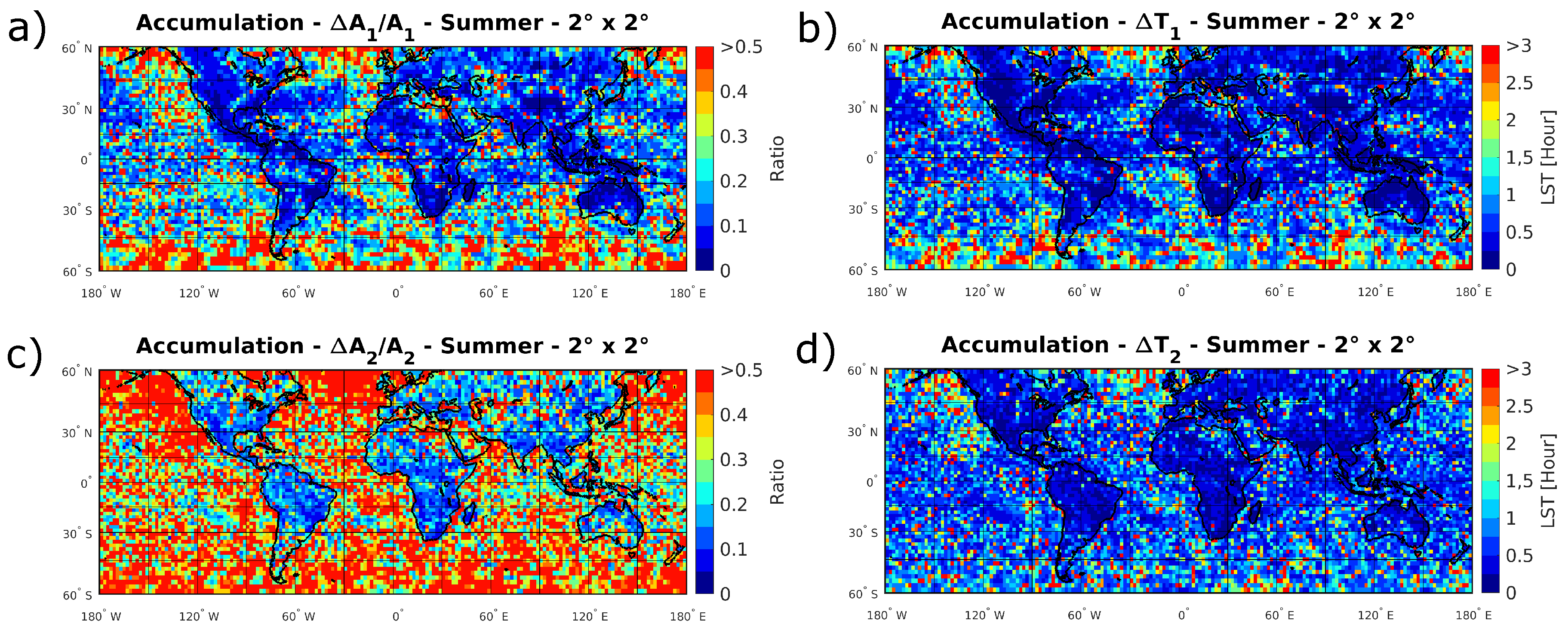
Figure 7.
Fitting errors on the harmonic parameters plotted in Figure 6. (a) The normalised fitting error on the amplitude of the 24 h harmonic; (b) the fitting error on the phase of the 24 h harmonic; (c) the normalised fitting error on the amplitude of the 12 h harmonic; (d) the fitting error on the phase of the 12 h harmonic. The caps on the colourbars represent the condition under which a parameter is considered unreliable.

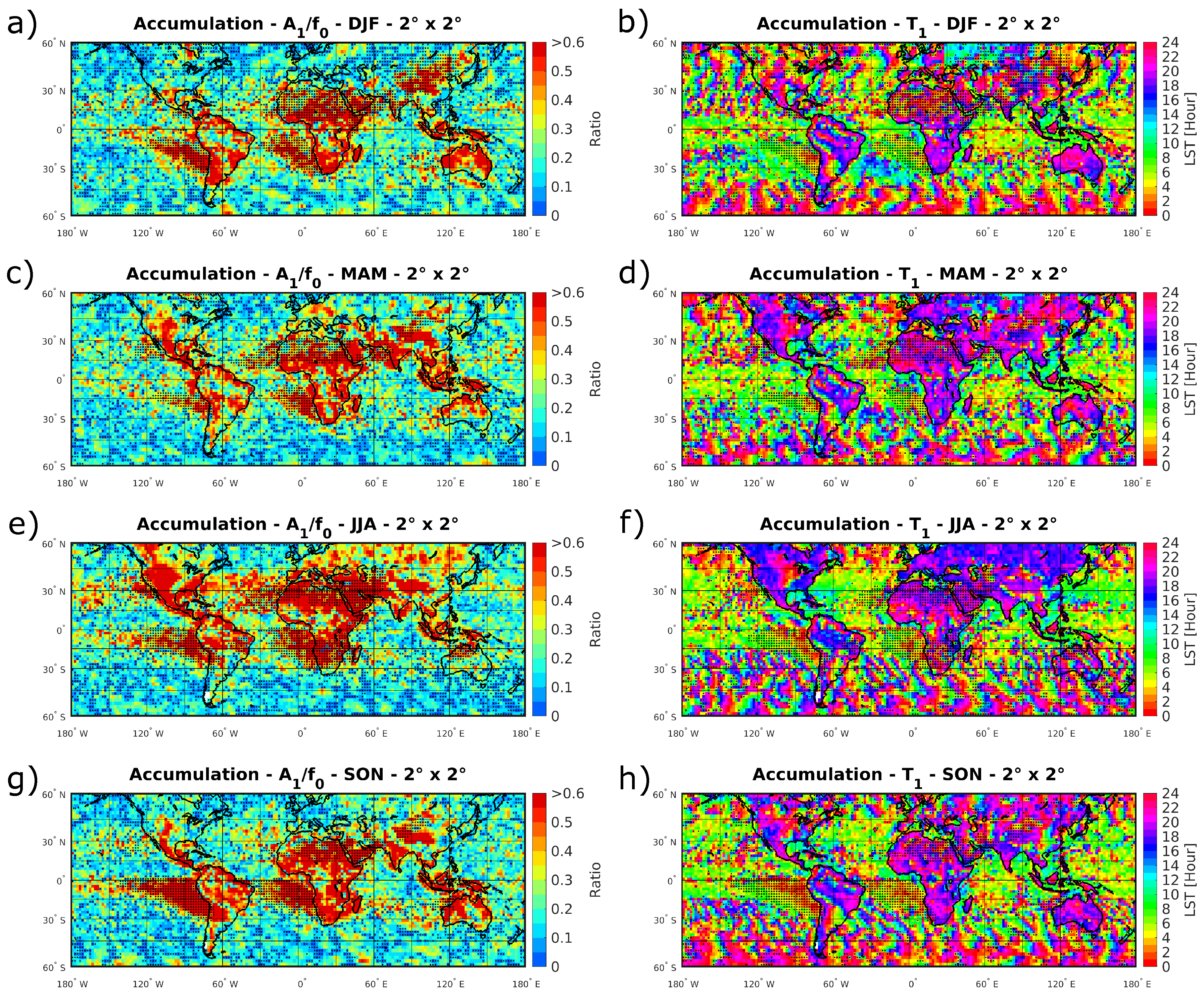
Figure 8.
Seasonal diurnal cycle of accumulation at resolution derived from four years of IMERG data, represented by (a,c,e,g) the amplitude of the 24 h harmonic normalized to the diurnal mean accumulation shown in Figure 3c; (b,d,f,h) the phase of the 24 h harmonic. Meteorological seasons are (a,b) December-January-February (DJF), (c,d) March-April-May (MAM), (e,f) June-July-August (JJA), and (g,h) September-October-November (SON). Refer to Section 2.2 for explanation of the blank and the black-dotted grid boxes.

© 2019 by the authors. Licensee MDPI, Basel, Switzerland. This article is an open access article distributed under the terms and conditions of the Creative Commons Attribution (CC BY) license (http://creativecommons.org/licenses/by/4.0/).
Share and Cite
MDPI and ACS Style
Watters, D.; Battaglia, A. The Summertime Diurnal Cycle of Precipitation Derived from IMERG. Remote Sens. 2019, 11, 1781. https://0-doi-org.brum.beds.ac.uk/10.3390/rs11151781
AMA Style
Watters D, Battaglia A. The Summertime Diurnal Cycle of Precipitation Derived from IMERG. Remote Sensing. 2019; 11(15):1781. https://0-doi-org.brum.beds.ac.uk/10.3390/rs11151781
Chicago/Turabian StyleWatters, Daniel, and Alessandro Battaglia. 2019. "The Summertime Diurnal Cycle of Precipitation Derived from IMERG" Remote Sensing 11, no. 15: 1781. https://0-doi-org.brum.beds.ac.uk/10.3390/rs11151781
Note that from the first issue of 2016, this journal uses article numbers instead of page numbers. See further details here.