New Strategies for Time Delay Estimation during System Calibration for UAV-Based GNSS/INS-Assisted Imaging Systems

Abstract

The need for accurate 3D spatial information is growing rapidly in many of today’s key industries, such as precision agriculture, emergency management, infrastructure monitoring, and defense. Unmanned aerial vehicles (UAVs) equipped with global navigation satellite systems/inertial navigation systems (GNSS/INS) and consumer-grade digital imaging sensors are capable of providing accurate 3D spatial information at a relatively low cost. However, with the use of consumer-grade sensors, system calibration is critical for accurate 3D reconstruction. In this study, ‘consumer-grade’ refers to cameras that require system calibration by the user instead of by the manufacturer or other high-end laboratory settings, as well as relatively low-cost GNSS/INS units. In addition to classical spatial system calibration, many consumer-grade sensors also need temporal calibration for accurate 3D reconstruction. This study examines the accuracy impact of time delay in the synchronization between the GNSS/INS unit and cameras on-board UAV-based mapping systems. After reviewing existing strategies, this study presents two approaches (direct and indirect) to correct for time delay between GNSS/INS recorded event markers and actual time of image exposure. Our results show that both approaches are capable of handling and correcting this time delay, with the direct approach being more rigorous. When a time delay exists and the direct or indirect approach is applied, horizontal accuracy of 1–3 times the ground sampling distance (GSD) can be achieved without either the use of any ground control points (GCPs) or adjusting the original GNSS/INS trajectory information.

1. Introduction

There is an increasing use of unmanned aerial vehicle (UAV)-based, global navigation satellite systems/inertial navigation systems (GNSS/INS)-assisted imaging systems among industries such as precision agriculture, infrastructure monitoring, emergency management, and defense. In particular, UAV imaging systems used in precision agriculture have a variety of applications, such as monitoring crops, estimating crop yield and best crop placement, and improving land cover classification. Use of UAVs in agricultural applications has expanded rapidly in recent years due to their relatively low cost and improved spatial and temporal resolution when compared to traditional satellite and manned aircraft imagery [1]. In addition, it is possible to equip UAVs with a variety of imaging sensors. These factors have increased the effectiveness of UAVs as a tool for precision agriculture and crop monitoring [2,3,4,5,6,7,8]. Additionally, RGB frame imagery can be useful for automating hyperspectral data orthorectification processes, allowing prediction of biomass and other phenotypic factors [9]. Thermal imagery has been used to estimate soil moisture, monitor evapotranspiration, and improve land cover classification [10,11,12,13,14]. Remotely sensed imagery has proven its usefulness in a wide range of agricultural environments. For many of these applications, remotely sensed imagery must be geo-referenced accurately. Proper system calibration is vital to providing accurate and actionable data for these applications.

System calibration of a UAV-based, GNSS/INS-assisted imaging system deals with both spatial and temporal aspects. Spatial system calibration aims at estimating both the internal characteristics of the camera, known as camera calibration, as well as system mounting parameters. Such parameters include principal point coordinates, principal distance, and distortion parameters for the internal camera characteristics and lever arm components, and boresight angles for the integration between GNSS/INS and multiple imaging sensors. The methodology behind camera calibration, either completed by manufactures in a laboratory setting or in a bundle adjustment with self-calibration, is well known [15,16,17,18]. In recent years, system calibration has become a focus of study. Describing the differences between the position and orientation of the GNSS/INS body frame and camera frames, lever arm components, and boresight angles, is key to system calibration. Lever arm and boresight calibration processes have also been well established by several research groups. Li et al. [19] worked on boresight calibration of both a mobile and UAV light detection and ranging (LiDAR) system using strip adjustment, while Habib et al. [20] completed rigorous boresight calibration for a UAV platform with a hyperspectral scanner equipped with GNSS/INS. Costa and Mitishita [21] focused on integrating photogrammetric and LiDAR datasets to improve sensor orientation information. However, even with accurate mounting parameters, precise time tagging between the imaging sensor and GNSS/INS unit is essential for accurate derivation of 3D spatial information. For consumer-grade systems, a time delay between image exposure and the corresponding GNSS/INS event recording might exist, and 3D spatial accuracy will be greatly reduced if this time delay is not taken into account. Throughout this manuscript, we will refer to the term “event marker,” which is used to indicate the time of exposure based on feedback signals received by the GNSS/INS unit from the camera. When time synchronization is not addressed and a time delay between the mid-exposure and GNSS/INS event marker exists, inaccuracies occur. As an example, an orthophoto generated using estimated system calibration parameters which did not include any time delay compensation, shown in Figure 1a, and the same orthophoto generated when the time delay was accounted for using the direct approach, which will be presented later in this paper, is shown in Figure 1b. In the highlighted area in Figure 1a, there are significant misalignments in the generated orthophoto. However, after time delay was compensated for within the bundle adjustment process, shown in Figure 1b, the generated orthophoto shows a smooth alignment in the same highlighted area as Figure 1a.

In addition to proper system calibration, the geo-referencing technique used in the system parameter estimation process is also important for providing accurate 3D information. There are a variety of techniques used for geo-referencing, which depend greatly on the application purpose, availability of resources, and accuracy requirements of the project. Direct and indirect geo-referencing are two main techniques used. Indirect geo-referencing uses aerial triangulation with the help of ground control points (GCPs) to accurately estimate system parameters. Indirect geo-referencing produces high accuracy, but is costly and time-consuming because of the need for GCPs in the triangulation [22,23]. On the other hand, direct geo-referencing uses a simple intersection adjustment and eliminates the need for GCPs, but can also reduce the overall accuracy of the system calibration. Several recent studies have focused on direct geo-referencing and the reduction or elimination of GCPs [24,25,26]. The accuracy of direct geo-referencing depends greatly on the onboard GNSS/INS unit and its integration within the rest of the imaging system, and without GCPs, degradation of geopositioning is a concern. The reduction or elimination of GCPs while ensuring high accuracy is a valuable prospect, considering it reduces cost, time, and equipment requirements when collecting data.

This study focused on system calibration of UAV-based, GNSS/INS-assisted imaging systems, specifically, studying calibration strategies capable of estimating time delay between GNSS/INS event markers and the image mid-exposure time. After review of existing strategies, we detail two approaches—direct and indirect—to solve for and correct this time delay. The direct approach uses a modified mathematical model to solve directly for the time delay in a bundle block adjustment. The direct approach modifies the bundle adjustment code for implementation. The indirect approach, on the other hand, exploits the correlation between the lever arm along the flying direction and the time delay—which follows from a less-than optimal flight configuration—as well the speed/time/distance relation to indirectly estimate time delay. The indirect approach exploits existing bundle adjustment code to estimate time delay. Section 2 focuses on related work, while Section 3 describes the methodology of the bundle block adjustment procedure, direct and indirect approaches, and optimal flight configuration for reliable estimation of the system calibration parameters. Section 4 focuses on description of the UAV-based imaging systems and data used in this study, in addition to experimental results and analysis. Lastly, Section 5 provides conclusions and recommendations for future research.

2. Related Work

Imaging systems used for obtaining accurate 3D spatial information need calibration both within the sensor and between the sensor and remaining system units. There has been a wide variety of calibration research over the years. Some research has focused on the sensor calibration itself and does not include the system parameters [27], whereas some system calibration research has focused not only on the internal characteristics of a sensor, but also the external and mounting parameters of the system as a whole [17,18]. Identifying features in imagery is also essential for calibration [28]. Many works have used distinct points, while others have used linear or planar features [18,29]. The type of control data used in previous calibration ranges from ground-based surveyed points, on-board GNSS/INS sensors, and superior sensor sources such as LiDAR. The accuracy associated with these types of control data used in calibration is approximately 3 mm for ground-based surveyed points, 8 mm planimetric accuracies for on-board GNSS/INS points, and 25 cm planimetric accuracy for LiDAR-derived control data [30,31,32]. Amongst this work, a variety of calibration parameters are of interest. As stated before, some are interested only in the internal characteristics of a sensor, while others are interested in full system calibration. Some of this research is strictly focused on the spatial calibration aspects of an imaging system, and neglects to address the temporal calibration.

As consumer-grade sensors integrated with GNSS/INS units on-board UAVs become more popular options for geospatial applications, the need to accurately estimate any time delay between GNSS/INS event marker and mid-exposure time during system calibration becomes increasingly important. Both hardware and software solutions have been introduced in an attempt to mitigate this problem. Elbahnasawy and Habib [33] introduced two hardware solutions to establish synchronization among different sensors, such as the recorded exposure time and the actual mid-exposure time. The authors discussed the simulated feedback approach, which uses a triggering system to send a signal to both the camera and the GNSS/INS unit simultaneously. The hypothesis of the simulated feedback approach is that the camera would capture the image at the same time the triggering signal is received. However, a camera does not capture an image instantaneously once the triggering signal is received. Therefore, the simulated feedback approach ignores the camera response time delay. Another hardware solution consists of using both a triggering signal, as described in the simulated feedback approach, and an optical clock to measure the camera response time [34]. The triggering signal is sent to the camera, GNSS/INS unit, and the optical clock. The function of the signal from the optical clock also sends a signal to the camera at an optional interval and begins counting with a graphical clock. The camera takes images of the optical clock counter and image processing, then determines the value displayed on the counter. The camera lag delay is then known. This approach assumes the time delay to be constant for future uses. Elbagnasawy and Habib’s [33] second approach, direct feedback, attempted to mitigate this camera response time delay further. The direct feedback approach utilizes the camera flash hot-shoe to generate a signal at the time the image is captured. This camera feedback signal is then sent to the GNSS/INS unit onboard, and a corresponding event time is recorded. One limitation to the direct feedback approach is that it assumes the hot-shoe flash signal corresponds exactly to the mid-exposure time. This cannot be assumed, and therefore a camera response time delay would still exist. Although hardware approaches can reduce the effects of time delay, it has proven to be difficult to record the actual mid-exposure. Furthermore, hardware modifications require both more time and monetary investment to implement. This may not be an option for all systems and applications. Therefore, others have investigated methods to measure time delay with software solutions. Recent software solutions for time delay estimation in imaging systems can be characterized into two categories. The first is one-step procedures that require a modification to bundle adjustment code. The second is two-step procedures that do not need modification to existing bundle adjustment code, but require two different independent adjustments.

Chiang et al. [30] proposed a calibration method to compensate for and estimate the magnitude of exposure time delay for a UAV-based imaging system. The authors introduced a two-step approach for estimating time delay. The interior orientation parameters (IOPs) are initially estimated through a camera calibration process. In the first step, the exterior orientation parameters (EOPs) are then estimated through indirect geo-referencing using GCPs. The differences in position and orientation between the EOPs and the interpolated trajectory from the on-board position and orientation system (POS) are derived. In the second step, the differences are then used in their calibration algorithm to solve for lever arm components, boresight angles, and time delay. Finally, the authors used the calibration parameters to perform direct geo-referencing applications without the need for GCPs. The results showed that by implementing the proposed calibration algorithm, a direct geo-positioning horizontal accuracy of 8 m at a flying height of 600 m and a 3D accuracy of 12 m can be achieved. The GSD while at 600 m flying height was 20 cm, and the camera had a pixel size of 0.0064 mm. Furthermore, the authors showed that the proposed calibration algorithm improved results by about 10% compared to traditional calibration. One limitation of the proposed algorithm is that a two-step process is needed—requiring two different independent adjustments—to produce results. EOPs are first derived through indirect geo-referencing with the help of GCPs, and the difference in position and rotation between the EOPs and the interpolated GNSS/INS solutions is calculated. Next, the calibration is completed by solving for mounting parameters and time delay. The algorithm also assumes that the rotation of the vehicle does not change during this time discrepancy. In their study, the measured time delay was between −0.107 and −0.227 s and the inertial measurement unit (IMU) rotation matrix was assumed to be constant during the delay. This assumption may not be valid, specifically when using lightweight UAV systems. Another disadvantage of this study is that it was sensitive to imaging/GCP/tie point configuration within the indirect geo-referencing step. Lastly, this study neglected the consideration of a suitable flight configuration for estimating time delay and ignored potential correlation among the EOPs and other unknowns.

Gabrlik et al. [31] proposed a similar two-step approach to that of Chiang et al. [30] for system calibration for estimating offset in lever arm, offset in GNSS/INS base station, and time delay for a UAV-based imaging system. In the first step of their approach, EOPs are estimated through indirect geo-referencing using Agisoft Photoscan Professional software [35]. The positional components of the EOPs are then considered the true positions of the images. Finally, the difference between the derived position from the GNSS receiver and the true position of an image is considered as a function of the system parameters mentioned above. Similar to Reference [30], this approach depends on the availability of GCPs to estimate ground truth for camera positions. However, compared to Reference [30], even when taking into consideration the differences in platform, sensor, and flying height, this approach did produce more accurate results, with RMSE in the XY component of 3.3 cm and 2.5 cm in the Z component. In addition, the proposed strategy did not consider any rotation variation information when estimating time delay.

Blazaquez, M. [36] introduced a new approach for one-step ‘spatio-temporal’ calibration of multi-sensor systems. This approach focuses on modifying the sensor model to include a time synchronization parameter. The approach uses the GNSS/INS-based linear and angular velocities to compute the displacement and orientation differences in estimating the time delay. Instead of solving for boresight angles, the author included a relative model that used the fact that if the sensor and IMU are rigidly attached, the relative rotation between two epochs is the same for both the sensor and the IMU. The author discussed the importance of varying linear velocity throughout the flight configuration for estimating the time delay parameter. However, because this specification was not met in their data collection, the data was manipulated to simulate strips being flown at different velocities. The absolute ‘spatio-temporal’ model produced RMS accuracy for check points in the 25–35 mm range. The approach also estimated the time synchronization parameter at the tenth of a millisecond precision level. The experiments relied on GCPs for accurate estimates of system calibration parameters, including time delay.

Rehak and Skaloud [34] worked on time synchronization of consumer cameras on micro aerial vehicles (MAVs). The author’s MAV system consisted of a Sony sensor that was initially modified to compensate for time synchronization issues between the camera and GNSS by using the direct feedback approach. The authors investigated two different methods for determining time delay within their system. The first method was an analysis of residuals between the observed camera positions and those estimated by indirect geo-referencing, which is a two-step process. The second method was a one-step approach to modify the mathematical model to include time delay as a parameter in the bundle adjustment. The second method used their absolute spatio-temporal model, with position, rotation, linear velocity, and angular velocity as observations. Both of these methods assume access to the position and velocity data from the GNSS/INS unit. A heuristic optimal flight configuration for estimating time delay was recommended. First, as part of the optimal configuration for system calibration while considering time delay, it was suggested that the lever arm be determined in a laboratory calibration, due to the correlation with the time delay. The overall optimal flight configuration then suggested that there must be a strong block configuration with both GNSS/INS in-flight data and ground control, high forward and side lap, variations in flying height and linear and angular velocities, and some obliquity in the imagery. The authors tested the validity of the methods through the evaluation of check points. During the evaluation experiment, nine check points were used in an integrated sensor orientation (ISO) with absolute aerial position observations. The results of this configuration showed an RMS of 56, 26, 54 mm in the X, Y, Z components, respectively, when the time events were corrected for a time delay of −6.2 ms. The interior orientation parameters and lever arm components were estimated in a separate calibration. The estimated time delay parameter ranged from −9.2 to −1.9 ms for the different methods.

3. Methodology

The presented approach in this study proposes two one-step algorithms: direct and indirect. The direct approach computes the linear and angular velocities directly and does not rely on raw data from the IMU. Additionally, to ensure the highest possible accuracy, the direct approach does not assume the platform rotation to be constant during the time delay period. The approaches were tested on systems with both sensors that were modified to incorporate the flash hot-shoe time synchronization—which significantly reduces the time delay—and also a sensor that only made use of the manufactured internal “frame sync” option. Furthermore, the approaches presented were tested and evaluated in an integrated sensor orientation (ISO) and direct geo-referencing adjustments, without the need for GCPs. Lastly, an optimal flight configuration was derived so that the system parameters, including the lever arm components, boresight angles, and time delay, could be estimated simultaneously. The optimal flight configuration presented maximizes the impact of biases or any possible errors in the system parameters, while also decoupling those parameters.

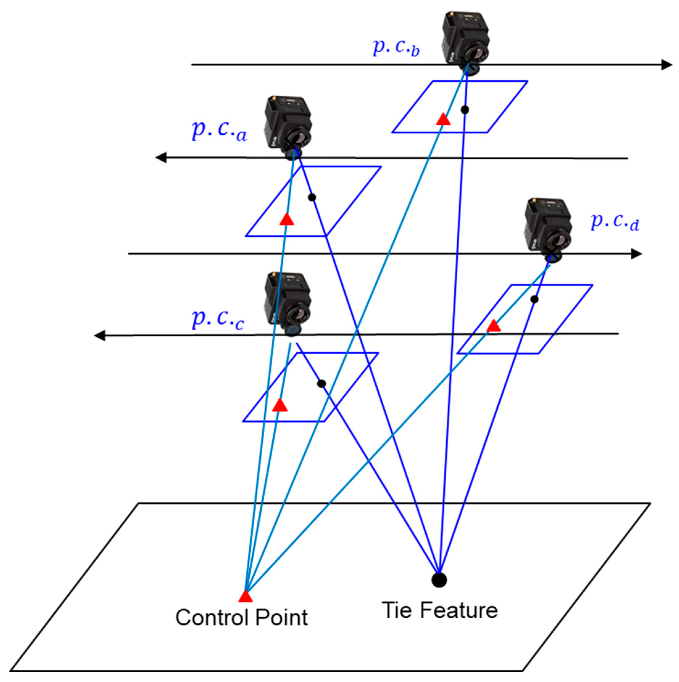
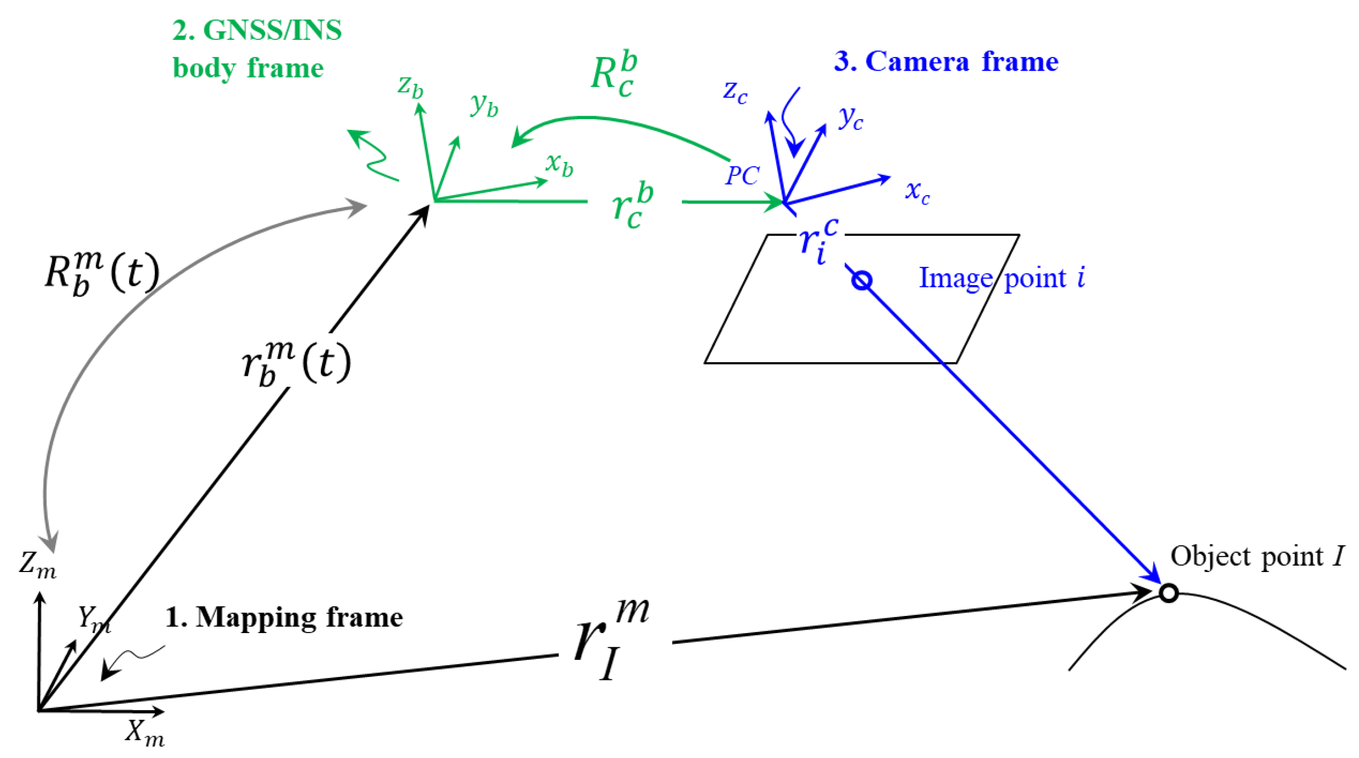
3.1. Conceptual Basis of Bundle Block Adjustment

For many photogrammetric applications, the goal is to increase accuracy while decreasing the required resources. The bundle block adjustment theory is a well-known method for increasing geospatial precision and accuracy derivation from imagery by improving geometric configuration and increasing redundancy while reducing the quantity of GCPs [15]. The bundle adjustment aims to ensure the best accuracy and precision of the reconstructed object space using minimal control. A graphical illustration of the bundle adjustment target function is presented in Figure 2. It promotes flexibility among solvable unknown parameters to suit individual user needs, and, in more recent years, it has been shown to be platform agnostic and capable of simultaneously combining a variety of sensors. Ravi et al. [37] used bundle adjustment theory to simultaneously perform system calibration of a multi-LiDAR/multi-camera mobile mapping platform. Habib et al. [18] demonstrated the use of bundle adjustment for self-calibration of line cameras using linear features detected in multiple datasets. Whether using frame or line cameras, or combining multiple sensors on a single/multiple platform(s), the mathematical model and overall least squares adjustment implementation of bundle adjustment is the same.

A UAV-based, GNSS/INS-assisted imaging system involves three coordinate systems: a mapping frame, an IMU body frame, and a camera frame. The mathematical model of the collinearity principle—which describes the collinearity of the camera perspective center, image point, and corresponding object point—is graphically illustrated and mathematically introduced in Figure 3 and Equation (1), respectively. The following notations are used throughout this study: a vector connecting point ‘b’ to point ‘a’ relative to a coordinate system associated with point ‘b’ is represented as $r_a^b$, and a rotation matrix transforming from coordinate system ‘a’ to coordinate system ‘b’ is represented as $R_a^b$.

$$r_I^m=r_{b\left(t\right)}^m+R_{b\left(t\right)}^m{r}_c^b+\lambda \left(i,c,t\right)R_{b\left(t\right)}^m{R}_c^b{r}_i^c$$

(1)

where:

• $r_I^m$: ground coordinates of the object point $I$
• $r_i^c=\left[\begin{array}{c}{x}_i-x_p-dis{t}_{x_i}\\ y_i-y_p-dis{t}_{y_i}\\ -c\end{array}\right]$: vector connecting perspective center to the image point
• $x_p,y_p$: principal point coordinates
• $c:$ principal distance
• $dis{t}_{x_i},dis{t}_{y_i}$: distortion in x and y directions for image point $i$
• $t$: time of exposure
• $r_{b\left(t\right)}^m$: position of IMU body frame relative to the mapping reference frame at time $t$ derived from the GNSS/INS integration process
• $R_{b\left(t\right)}^m$: rotation matrix from the IMU body frame to the mapping reference frame at time $t$ derived from the GNSS/INS integration process
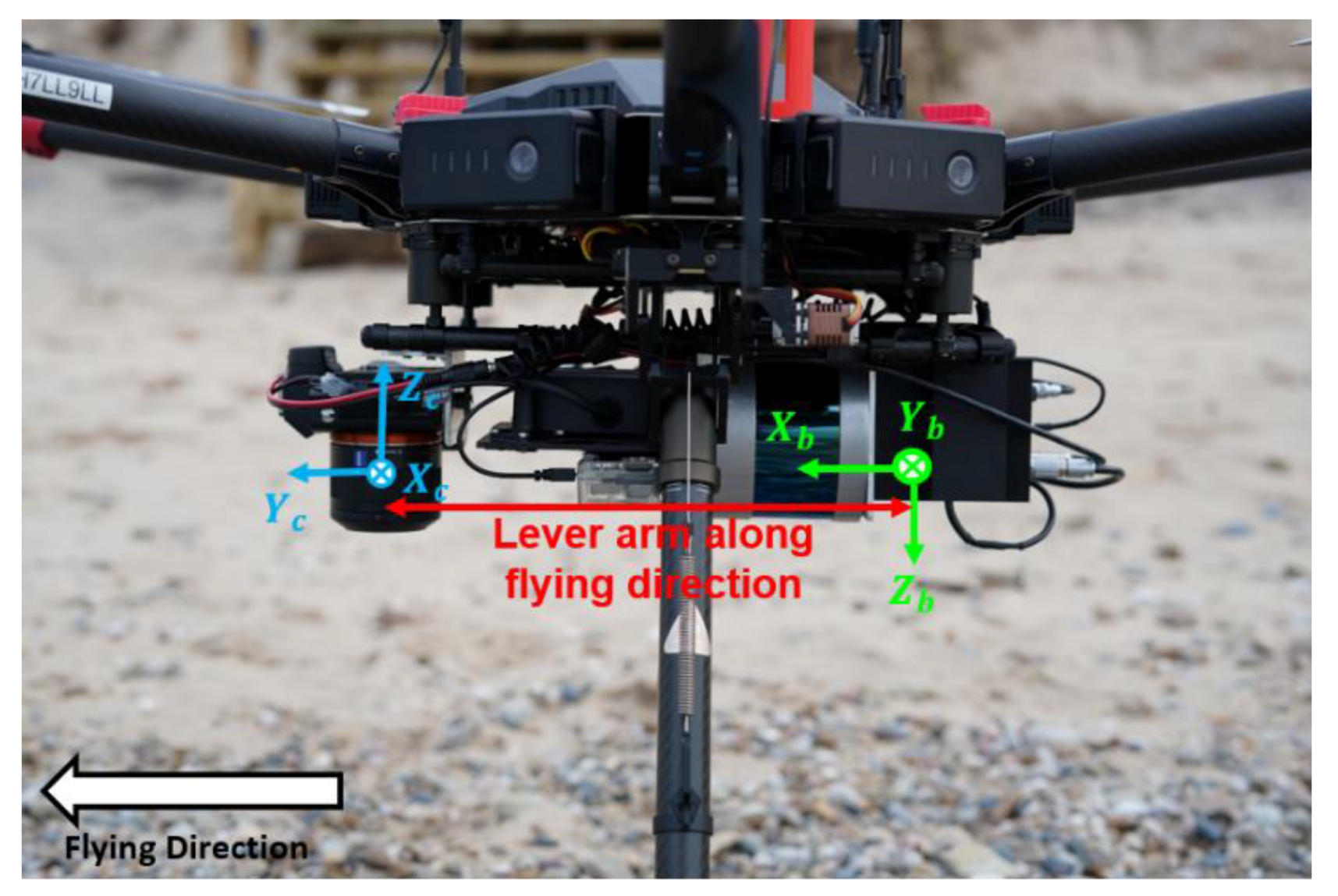
• $r_c^b$: lever arm from camera to IMU body frame
• $R_c^b$: rotation (boresight) matrix from camera to IMU body frame
• $\lambda \left(i,c,t\right)$: scale factor for point $i$ captured by camera $c$ at time t

Reformulating Equation (1), one can represent image coordinates as a function of the GNSS/INS position and orientation, ground coordinates of GCPs/tie points, lever arm components, and the boresight matrix, as shown in Equation (2).

$$r_i^c=\frac{1}{\lambda \left(i,c,t\right)}{R}_b^c\left[R_m^{b\left(t\right)}\left[r_I^m-r_{b\left(t\right)}^m\right]-r_c^b\right]=\frac{1}{\lambda \left(i,c,t\right)}\left[\begin{array}{c}{N}_x\\ N_y\\ D\end{array}\right]$$

(2)

where:

$$\left[\begin{array}{c}{N}_x\\ N_y\\ D\end{array}\right]=R_b^c\left[R_m^{b\left(t\right)}\left[r_I^m-r_{b\left(t\right)}^m\right]-r_c^b\right]$$

To eliminate the unknown scale factor $\lambda \left(i,c,t\right)$ from Equation (2), the first and second rows can be divided by the third one to produce Equations (3a) and (3b) [15], which are nonlinear forms in the unknowns, including system calibration.

$$x_i-x_p-dis{t}_{x_i}=-c\frac{N_x}{D}$$

(3a)

$$y_i-y_p-dis{t}_{y_i}=-c\frac{N_y}{D}$$

(3b)

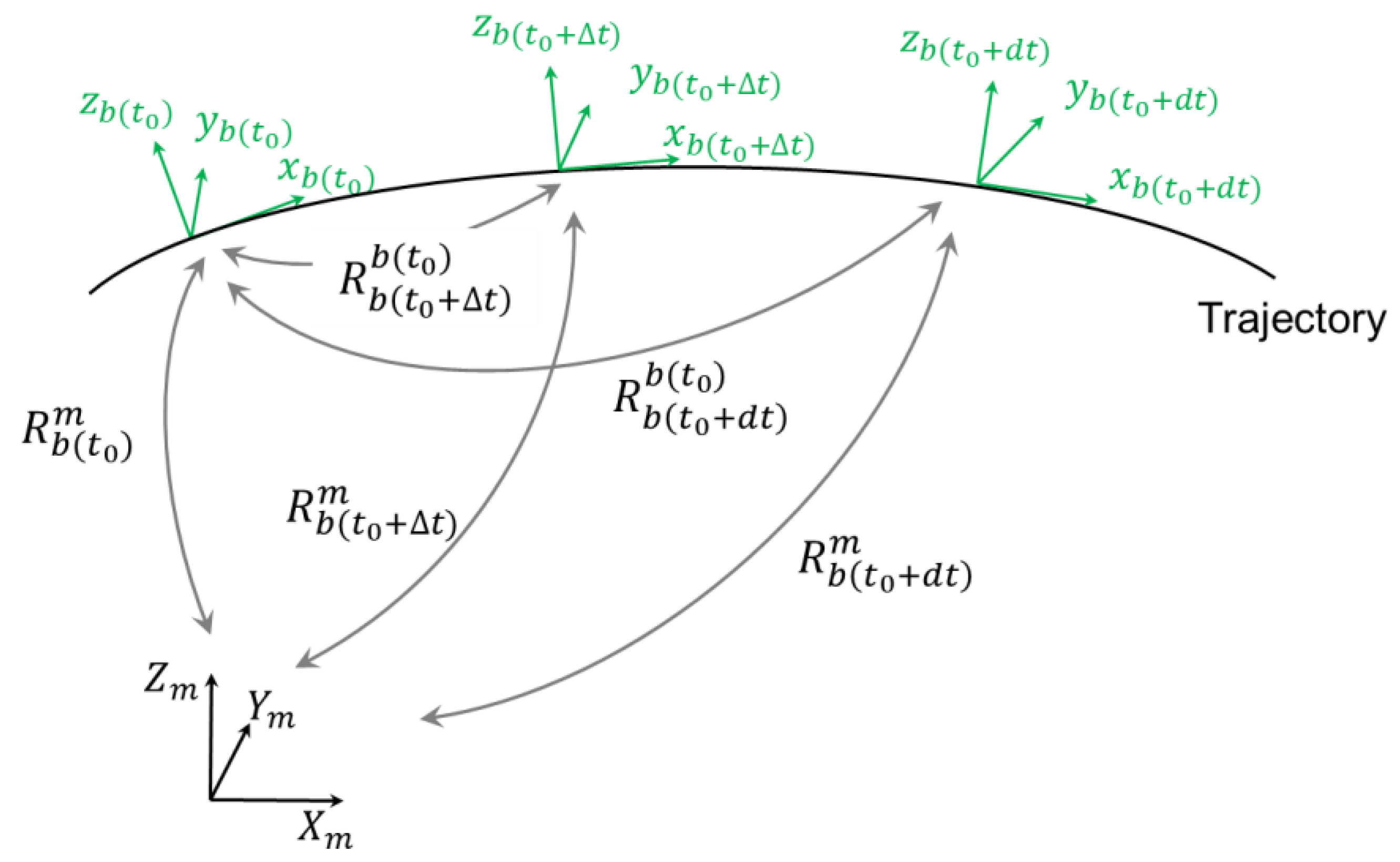
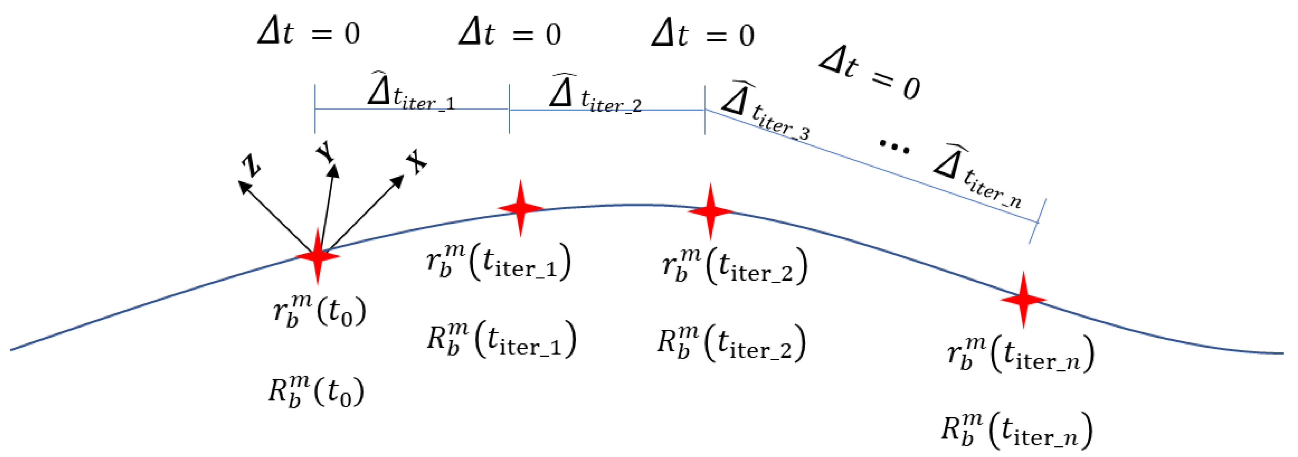
3.2. Direct Approach for Time Delay Estimation

The first strategy for time delay estimation introduced in this study is the direct approach, where the time delay is directly estimated in a bundle adjustment with the system self-calibration process. The previously discussed mathematical model is modified to incorporate the time delay parameter, and is derived as explained below.

Given the position and orientation at $t_0$, initial event marker time, the objective is to find the correct position and orientation at the actual mid-exposure time, $t$, by taking into account the time (delay), $\Delta t$, between actual exposure time and initial event marker time. It follows that the actual time of exposure equals the initial event marker time plus the time delay, $t=t_0+\Delta t$. Based on the collinearity Equation (1), it is clear that a time delay between the mid-exposure and the recorded event marker by the GNSS/INS unit will directly affect the position $r_{b\left(t\right)}^m$ and orientation $R_{b\left(t\right)}^m$ of the body frame. Therefore, one must estimate the changes in position and orientation caused by the time delay. The position at the correct time, $r_{b\left(t\right)}^m$, can then be expressed by using the position at the initial event marker time tag and adding the displacement caused by the time delay, expressed in Equation (4). The instantaneous linear velocity, $\dot{r}{}_{b\left(t_0\right)}^m$, at the initial event marker time is needed to calculate the displacement. The instantaneous linear velocity is expressed in Equation (5). It should be noted that the GNSS and IMU units typically have data rates of 10 and 200 Hz, respectively. The GNSS/INS integration process produces the position and orientation of the IMU body frame at a given time interval, which is usually interpolated to that of the data rate of the IMU, which was 200 Hz in this study. Given this trajectory, we specify a time interval, $dt$, which we use to compute the instantaneous linear, and later the angular velocity. The interpolation frequency chosen is controlled by the data rate of the IMU unit and the expected noise level in the derived trajectory. Choosing a very high frequency for the interpolation will magnify the impact of noise. The frequency of the interpolation process is balanced to consider both the data rate of the data acquisition system as well as reducing the impact of the noise in the derived trajectory.

$$r_{b\left(t\right)}^m=r_{b\left(t_0\right)}^m+\Delta t{\dot{r}}_{b\left(t_0\right)}^m$$

(4)

$${\dot{r}}_{b\left(t_0\right)}^m=\frac{1}{dt}[r_{b\left(t_0+dt\right)}^m-r_{b\left(t_0\right)}^m]$$

(5)

Next, an expression for the orientation of the IMU body frame, $R_{b\left(t\right)}^m$, at the correct mid-exposure time can be derived. Deriving an expression for the orientation of the IMU body frame at the correct mid-exposure time enables the direct approach to handle rotational variation during the time delay. Here, we examine the changes in the rotation of the IMU body frame at different times. With the help of Figure 4, we can see that the rotation matrix at the correct exposure time, $R_{b\left(t\right)}^m$, can be derived from the rotation of the body frame at time $t_0$, as well as the angular velocity and time delay. The angular velocity is derived based on the rotation at time $t_0$ and rotation at time $t_0+dt$, as shown in Equation (6). More specifically, we can use the rotation at time $t_0$ and the rotation at time $t_0+dt$ to derive the changes in the rotation angles denoted by $d{\omega }_b\left(t_0\right)$, $d{\phi }_b\left(t_0\right)$, and $d{\kappa }_b\left(t_0\right)$. These rotation changes, along with the user-defined time interval, $dt$, can then be used to derive the angular velocity, as per Equation (7a–c). Using the angular velocities and the time delay, the change in rotation caused by the existing time delay can be derived, as shown in Equation (8). It should be noted that an expression for the incremental rotation matrix is used in Equation (8), since the angular change caused by the time delay is relatively small. Finally, using the IMU body orientation at the initial event marker time, expressed as $R_{b\left(t_0\right)}^m$, along with the rotation changes during the time delay, expressed as $R_{b\left(t_0+\Delta t\right)}^{b\left(t_0\right)}$, the IMU body orientation at the actual exposure time, $R_{b\left(t\right)}^m$, can be derived, as per Equation (9). Substituting Equations (4) and (9) into Equation (1), the collinearity equations can be rewritten as in Equation (10).

$$R_{b\left(t_0+dt\right)}^{b\left(t_0\right)}=R_m^{b\left(t_0\right)}{R}_{b\left(t_0+dt\right)}^m=Rotation\left(d{\omega }_b\left(t_0\right),d{\phi }_b\left(t_0\right),d{\kappa }_b\left(t_0\right)\right)$$

(6)

$${\dot{\omega }}_b\left(t_0\right)=\frac{d{\omega }_b\left(t_0\right)}{dt}$$

(7a)

$${\dot{\omega }}_b\left(t_0\right)=\frac{d{\omega }_b\left(t_0\right)}{dt}$$

(7b)

$${\dot{\kappa }}_b\left(t_0\right)=\frac{d{\kappa }_b\left(t_0\right)}{dt}$$

(7c)

$$\begin{array}{l}{R}_{b\left(t_0+\Delta t\right)}^{b\left(t_0\right)}=Rotation\left({\dot{\omega }}_{b\left(t_0\right)}\Delta t,{\dot{\phi }}_{b\left(t_0\right)}\Delta t,{\dot{\kappa }}_{b\left(t_0\right)}\Delta t\right)\\ \cong \left[\begin{array}{ccc}1& -{\dot{\kappa }}_b\left(t_0\right)\Delta t& {\dot{\phi }}_b\left(t_0\right)\Delta t\\ {\dot{\kappa }}_b\left(t_0\right)\Delta t& 1& -{\dot{\omega }}_b\left(t_0\right)\Delta t\\ -{\dot{\phi }}_b\left(t_0\right)\Delta t& {\dot{\omega }}_b\left(t_0\right)\Delta t& 1\end{array}\right]\end{array}$$

(8)

$$R_{b\left(t\right)}^m=R_{b\left(t_0\right)}^m{R}_{b\left(t_0+\Delta t\right)}^{b\left(t_0\right)}$$

(9)

$$r_i^c=\frac{1}{\lambda \left(i,c,t\right)}{R}_b^c\left[R_{b\left(t_0\right)}^{b\left(t_0+\Delta t\right)}{R}_m^{b\left(t_0\right)}\left(r_I^m-r_{b\left(t_0\right)}^m-{\dot{r}}_{b\left(t_0\right)}^m\Delta t\right)-r_c^b\right]$$

(10)

The mathematical model is now modified so that the image coordinate measurements are a function of the trajectory information, IOPs, lever arm components, boresight angles, ground coordinates, and time delay. More specifically, during the least squares adjustment, time delay is treated as an unknown parameter. The initial value of time delay is set to zero. The first iteration is performed and the lever arm components, boresight angles, ground coordinates of tie points, and time delay are solved for. The time delay is applied to adjust the IMU body frame position and orientation for the next iteration, and the time delay is set back to zero before the next iteration. The iterations continue until the time delay estimate is approximately zero and the corrections to the other unknown parameters are sufficiently small, as illustrated by Figure 5.

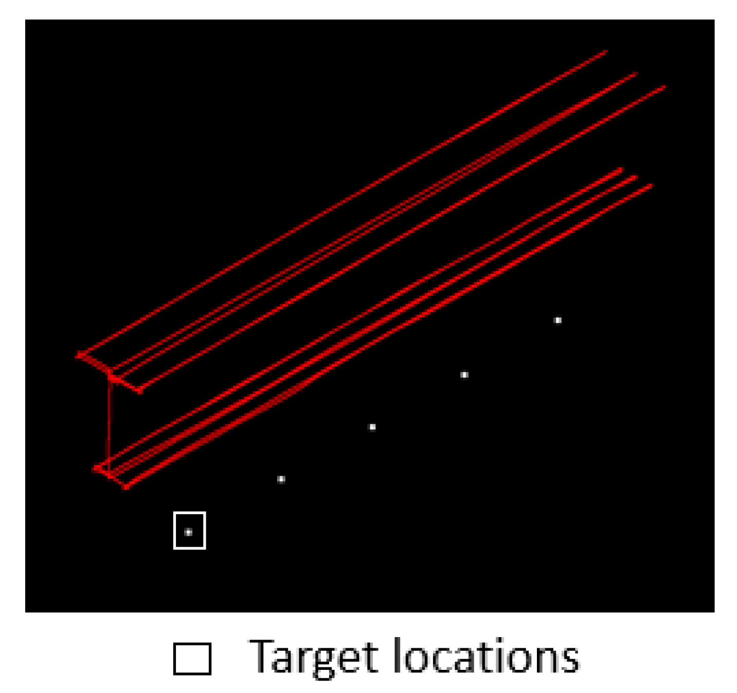
3.3. Optimal Flight Configuration for System Calibration while Considering Time Delay

The objective of this section is to determine an optimal flight configuration that results in an accurate estimation of the system parameters, including the lever arm components, boresight angles, and time delay. The optimal flight configuration is the one that maximizes the impact of biases or any possible errors in the system parameters while also decoupling those parameters. A rigorous approach for doing this is to derive the impact of biases in the system parameters on the derived ground coordinates. Bias impact analysis can be done by deriving the partial derivatives of the point positioning equation with respect to the system parameters. Equation (11) reformulates Equation (10) to express the ground coordinates as a function of the measurements and system parameters. Partial derivatives are derived from Equation (11).

For system calibration, the unknown parameters, denoted henceforth by x, consist of the lever arm components, $\Delta X,\Delta Y,\Delta Z$, boresight angles, $\Delta \omega ,\Delta \phi ,\Delta \kappa$, and time delay, $\Delta t$. Generalizing Equation (11) to Equation (12), we can see that the ground coordinate, $r_I^m,$ is a function of the system parameters, x. Taking the partial derivatives of the collinearity equations with respect to each system parameter and multiplying by the discrepancy in the system parameters, $\delta x$, shows which flight configuration produces a change in the ground coordinates, $\delta r_I^m$, as expressed in Equation (13).

$$r_I^m=r_{b\left(t_0\right)}^m+{\dot{r}}_{b\left(t_0\right)}^m\Delta t+R_{b\left(t_0\right)}^m{R}_{b\left(t_0+\Delta t\right)}^{b\left(t_0\right)}{r}_c^b+\lambda \left(i,c,t\right)R_{b\left(t_0\right)}^m{R}_{b\left(t_0+\Delta t\right)}^{b\left(t_0\right)}{R}_c^b{r}_i^c$$

(11)

$$r_I^m=f\left(x\right)$$

(12)

$$\delta r_I^m=\frac{\partial r_I^m}{\partial x}\delta x$$

(13)

where:

$$\delta x=\left(\delta \Delta X,\delta \Delta Y,\delta \Delta Z,\delta \Delta \omega ,\delta \Delta \phi ,\delta \Delta \kappa ,\delta \Delta t\right)$$

To simplify this analysis, we make a few assumptions. These assumptions are specifically made to simplify the derivation, and the analysis of the bias impact is not affected if such assumptions are not met. It should be noted that deviations from these assumptions would have a more favorable effect on our ability to decouple the impact of various system parameters. We assume that the sensor is traveling with a constant attitude in the south-to-north and north-to-south directions. Throughout this manuscript, we use double signs, $\pm$ and $\mp$, to refer to the direction of the flight. The top sign pertains to south-to-north flight and the bottom sign refers to north-to-south flight. We also assume that the sensor and IMU body frame coordinate systems are vertical. Therefore, we also assume that the sensor and IMU body frame coordinate systems are almost parallel. Lastly, we assume that we are flying over flat, horizontal terrain, where the scale is equal to the flying height over the principal distance, $=\frac{H}{c}$.

Now that these assumptions are established, we compute the partial derivatives with respect to each system parameter. Examining Equation (11), we can see that there are three terms that are comprised of system parameters and are needed to compute the partial derivatives, namely ${\dot{r}}_{b\left(t_0\right)}^m\Delta t,$ $R_{b\left(t\right)}^m{r}_c^b$ and $\lambda \left(i,c,t\right)R_{b\left(t\right)}^m{R}_c^b{r}_i^c.$ The first term, ${\dot{r}}_{b\left(t_0\right)}^m\Delta t,$ only includes the time delay system parameter, and its partial derivative will simply be the instantaneous linear velocity. Based on the sensor flight direction assumption and the incremental rotation resulting from the time delay, shown in Equation (8), we can expand $R_{b\left(t\right)}^m$ to the form in Equation (14). Using the assumption that the sensor to IMU–body frame lever arm is small, second order incremental terms in $R_{b\left(t\right)}^m{r}_c^b$ are ignored; using Equation (14), $R_{b\left(t\right)}^m{r}_c^b$ can then be expressed as in Equation (15). Next, after multiplication of the image coordinate vector, boresight matrix, IMU body frame rotation matrix, and scale factor, the third term, $\lambda \left(i,c,t\right)R_{b\left(t\right)}^m{R}_c^b{r}_i^c,$ is expressed in Equation (16), where second order incremental terms are again ignored. From Equations (15) and (16), we explicitly have the terms needed for the partial derivatives.

$$\begin{array}{ll}{R}_{b\left(t\right)}^m& =\left[\begin{array}{ccc}\pm 1& 0& 0\\ 0& \pm 1& 0\\ 0& 0& 1\end{array}\right]\left[\begin{array}{ccc}1& -{\dot{\kappa }}_b\left(t_0\right)\Delta t& {\dot{\phi }}_b\left(t_0\right)\Delta t\\ {\dot{\kappa }}_b\left(t_0\right)\Delta t& 1& -{\dot{\omega }}_b\left(t_0\right)\Delta t\\ -{\dot{\phi }}_b\left(t_0\right)\Delta t& {\dot{\omega }}_b\left(t_0\right)\Delta t& 1\end{array}\right]\\ & =\left[\begin{array}{ccc}\pm 1& \mp {\dot{\kappa }}_b\left(t_0\right)\Delta t& \pm {\dot{\phi }}_b\left(t_0\right)\Delta t\\ \pm {\dot{\kappa }}_b\left(t_0\right)\Delta t& \pm 1& \mp {\dot{\omega }}_b\left(t_0\right)\Delta t\\ -{\dot{\phi }}_b\left(t_0\right)\Delta t& {\dot{\omega }}_b\left(t_0\right)\Delta t& 1\end{array}\right]\end{array}$$

(14)

$$R_{b\left(t\right)}^m{r}_c^b=\left[\begin{array}{c}\pm \Delta X\\ \pm \Delta Y\\ \Delta Z\end{array}\right]$$

(15)

$$\lambda \left(i,c,t\right)R_{b\left(t\right)}^m{R}_c^b{r}_i^c=\lambda \left(i,c,t\right)\left[\begin{array}{c}\pm x_i\mp y_i\Delta \kappa \mp {\dot{\kappa }}_b\left(t_0\right)y_i\Delta t\mp c\Delta \phi \mp {\dot{\phi }}_b\left(t_0\right)c\Delta t\\ \pm {\dot{\kappa }}_b\left(t_0\right)x_i\Delta t\pm x_i\Delta \kappa \pm y_i\pm c\Delta \omega \mp {\dot{\omega }}_b\left(t_0\right)c\Delta t\\ -{\dot{\phi }}_b\left(t_0\right)x_i\Delta t-x_i\Delta \phi +{\dot{\omega }}_b\left(t_0\right)y_i\Delta t+y_i\Delta \omega -c\end{array}\right]$$

(16)

The partial derivatives needed for the bias impact analysis are those relative to the lever arm components, boresight angles, and time delay. These partial derivatives, derived from Equations (15) and (16), are expressed in Equation (17a–c). Examining these partial derivatives, one can see which dependencies these system parameters exhibit. The impact of the lever arm component changes depends on the flying direction. The impact of the boresight angles on the ground coordinates is a function of the flying height, flying direction, and the ratio of the image point coordinates and the principal distance, $\frac{x_i}{c}$ and $\frac{y_i}{c}$. Lastly, the impact of the time delay is a function of the linear and angular velocities, scale, image point coordinates, principal distance, and flying direction. The dependency of the bias impact for the system calibration parameters on image point location, flying direction, flying height, and linear and angular velocity is summarized in

Table 1. Dependency of the bias impact for the system calibration parameters on flight configuration and image point location.

System Parameter	Image Point Location	Flying Direction	Flying Height	Linear Velocity	Angular Velocity
Lever Arm	NO	YES (except ΔZ)	NO	NO	NO
Boresight	YES	YES	YES	NO	NO
Time Delay	YES (only in the presence of angular velocities)	YES	YES (only in the presence of angular velocities)	YES	YES

.

$$\delta r_I^m{\mid }_{\delta r_c^b}=\left[\begin{array}{c}\pm \delta \Delta X\\ \pm \delta \Delta Y\\ \delta \Delta Z\end{array}\right]$$

(17a)

$$\delta r_I^m{\mid }_{\delta \Delta \omega ,\delta \Delta \phi ,\delta \Delta \kappa }=H\left[\begin{array}{c}\pm \frac{x_i{y}_i}{c^2}\delta \Delta \omega \mp \left(1+\frac{x_i{}^2}{c^2}\right)\delta \Delta \phi \mp \frac{y_i}{c}\delta \Delta \kappa \\ \pm \left(1+\frac{y_i^{}{}^2}{c^2}\right)\delta \Delta \omega \mp \frac{x_i{y}_i}{c^2}\delta \Delta \phi \pm \frac{x_i}{c}\delta \Delta \kappa \\ 0\end{array}\right]$$

(17b)

$$\delta r_I^m{\mid }_{\delta \Delta t}={\dot{r}}_{b\left(t_0\right)}^m\delta \Delta t+\lambda \left(i,c,t\right)\left[\begin{array}{c}\pm {\dot{\kappa }}_b\left(t_0\right)y_i\delta \Delta t\mp {\dot{\phi }}_b\left(t_0\right)c\delta \Delta t\\ \pm {\dot{\kappa }}_b\left(t_0\right)x_i\delta \Delta t\mp {\dot{\omega }}_b\left(t_0\right)c\delta \Delta t\\ -{\dot{\phi }}_b\left(t_0\right)x_i\delta \Delta t+{\dot{\omega }}_b\left(t_0\right)y_i\delta \Delta t\end{array}\right]$$

(17c)

Now that we know which system parameters produce a change in ground coordinates, and whether that change depends on the image point location, flying direction, flying height, and/or linear/angular velocity, we then design the optimal flight configuration for system calibration while considering time delay. As a result of this analysis we can conclude that the horizontal components of the lever arm can be estimated using different flying directions, while its vertical component is independent of flight configuration. On the other hand, to estimate boresight angles while decoupling them from lever arm components, different flying directions and flying heights are needed, as well as a good distribution of image points. Finally, to derive the time delay and decouple this parameter from the lever arm components and boresight angles, variation in linear/angular velocity and a good distribution of image points are required. In summary, it is recommended to derive the system parameters using opposite flying directions at different flying heights, as well as having a variation in the linear and angular velocities and good distribution of the image points. It should be emphasized that the assumptions imposed while deriving the minimal optimal flight configurations were only made to simplify the derivations and are not requirements for the presented approaches or experiments. If these assumptions are not met, the analysis of bias impact is not affected. Furthermore, any deviations from the abovementioned assumptions will lead to a more favorable impact on the ability to decouple system parameters. It should be noted that variation in the angular velocity might be difficult to control. However, for small, multi-rotor UAVs, angular velocity variation might be present. Using the optimal flight configuration, systematic errors can be easily detected, estimated, and removed, therefore resulting in more accurate 3D reconstruction.

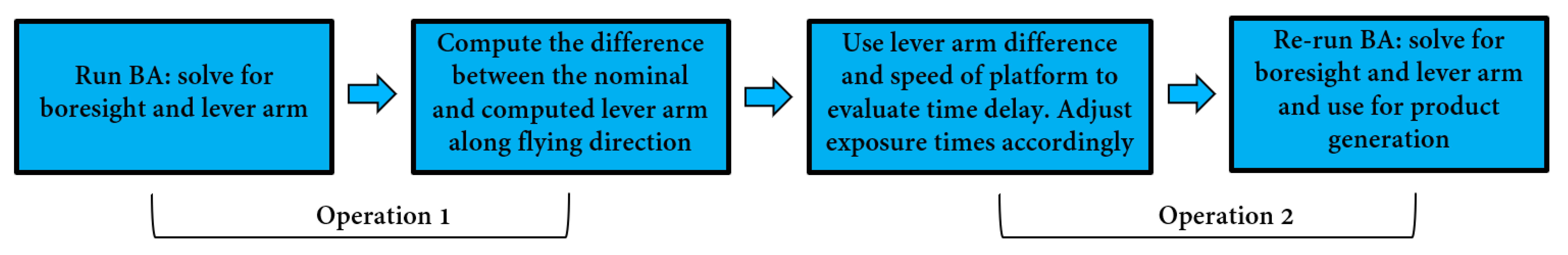
3.4. Indirect Approach for Time Delay Estimation

The next approach we propose to evaluate time delay is the indirect approach. This approach uses the above bias impact analysis by exploiting the fact that the lever arm component in the flying direction is correlated with the time delay, given a single linear velocity and insignificant angular velocity. In other words, if flights in opposite directions and constant linear velocity are used, then the lever arm component in the flying direction will be correlated with the time delay. As a result, by estimating the lever arm component in the flying direction, while not considering the time delay, and then comparing it with the nominal value which can be directly measured from the GNSS/INS unit to the imaging sensor, one can discern the existence of a possible time delay in system synchronization. An illustration of where measurements are taken to acquire the nominal lever arm values is shown in Figure 6. This approach is meant as a special case in which one chooses to use an existing bundle adjustment with system self-calibration mechanism to estimate time delay, instead of incorporating the time delay as a parameter and implementing the direct approach.

The indirect approach consists of a single bundle adjustment, with the system self-calibration operation completed twice. In the first operation, an initial GNSS/INS-assisted bundle adjustment is performed to solve for the lever arm components (only lever arm in the flying direction) and boresight angles. If a significant time delay exists, the computed lever arm in the flying direction will be quite different from the nominal value. This will be the first hint that the system may have a time delay issue. After the initial bundle adjustment is performed, the difference between the computed lever arm and the nominal/measured lever arm in the flying direction is derived. In the second operation, this difference in distance is now known and the time delay can be computed using the speed/time/distance relation. The computed time delay is then applied to derive the new position and orientation of IMU body frame at the actual exposure time. Finally, another bundle adjustment is performed to solve for the mounting parameters. Figure 7 presents the processing workflow of this approach.

In summary, the bundle block adjustment and mathematical model does not change from the traditional GNSS/INS-assisted bundle adjustment with system self-calibration procedure, expressed in Equation (3). The image coordinates are still a function of the trajectory information, IOPs, lever arm components, boresight angles, and ground coordinates. The time delay is not directly derived, but indirectly estimated using the lever arm deviation in the along flight direction and the speed/time/distance relation. However, one limitation of this approach is that because we are making the assumption that the time delay impact is absorbed by the lever arm in the flying direction, we have to fly at a single linear velocity. Additionally, because this approach only considers the impact of time delay on the lever arm component, it ignores the possibility of rotation changes during the time delay (i.e., angular velocity). Therefore, the calibration results may be less accurate than using the direct approach and an optimal flight configuration. However, the key advantage for the indirect approach is that it is capable of using existing bundle adjustment software to estimate the time delay in the system.

4. Experimental Results

In this section, data acquisition is discussed first, which includes information about the platforms and imaging systems used in this study. Next, the dataset description is presented. This description includes information on the flight configuration and ground control points collected. Finally, the experimental results and analysis are discussed. Each experiment and its results are presented in detail, along with an analysis discussion.

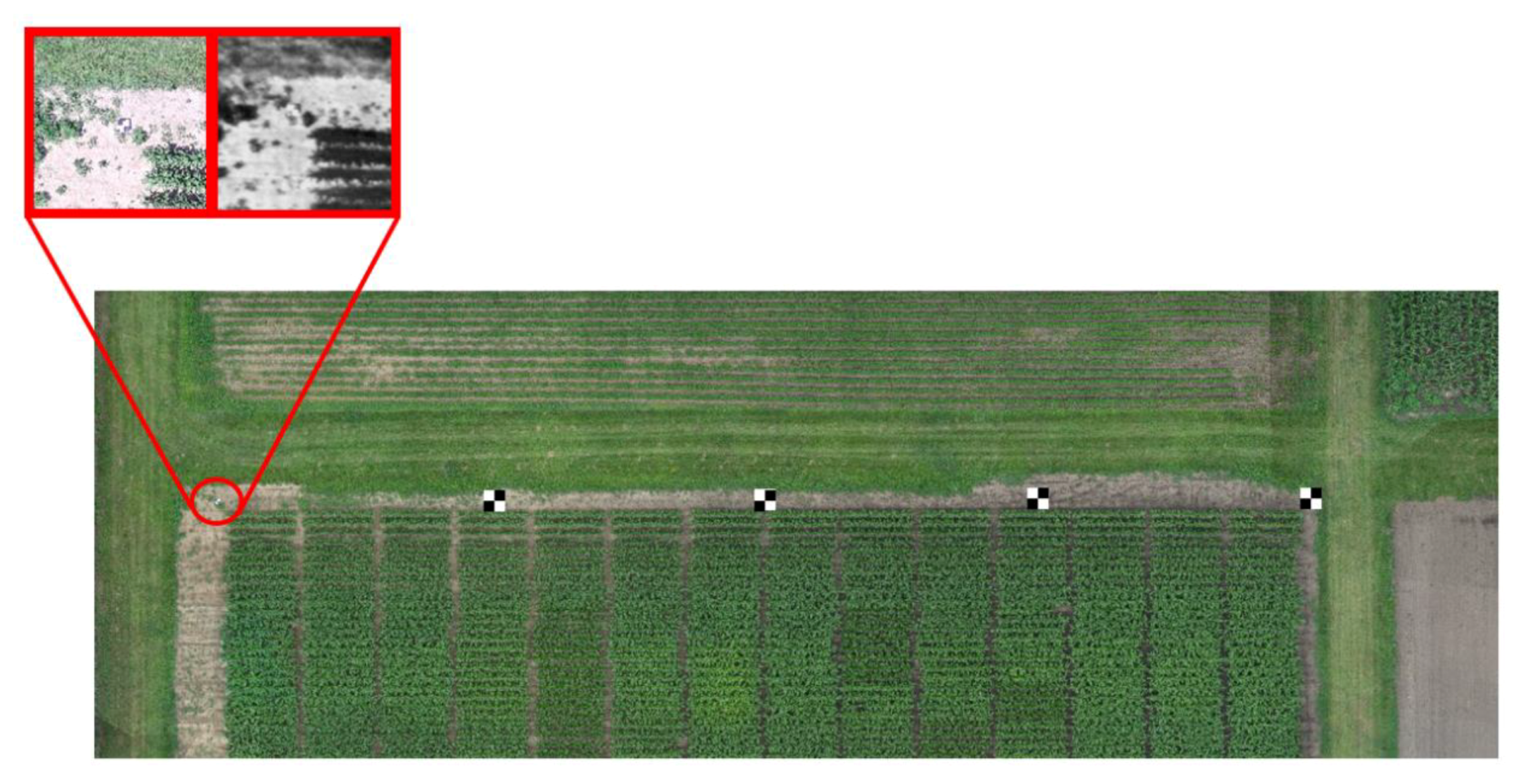
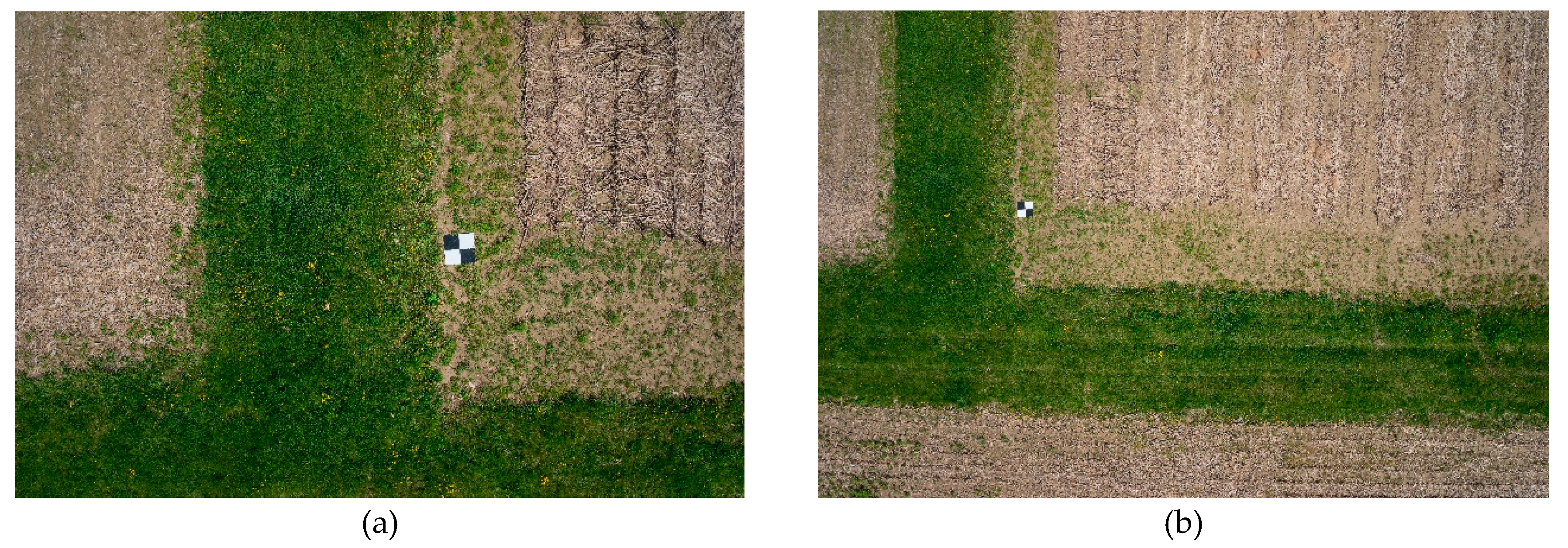
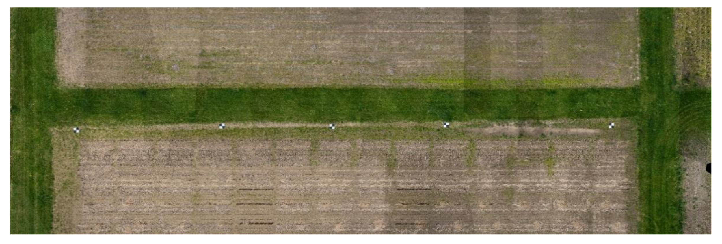
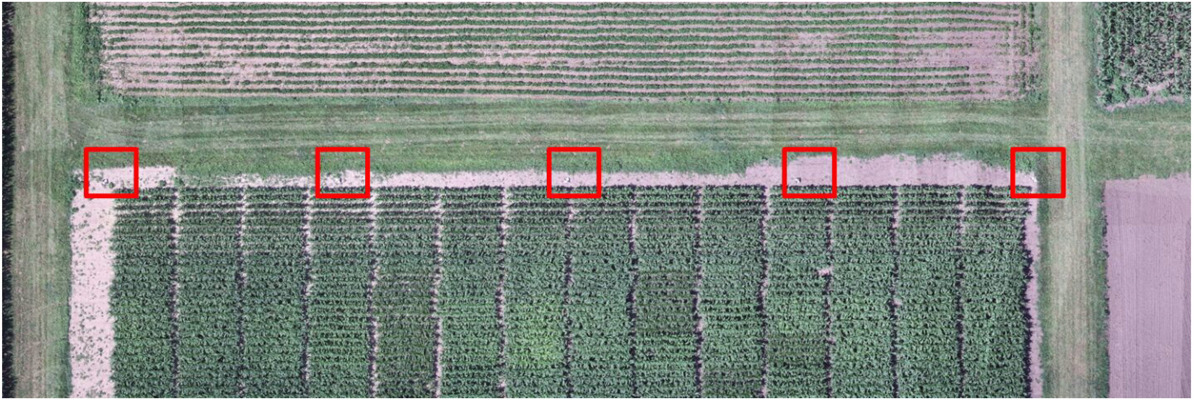
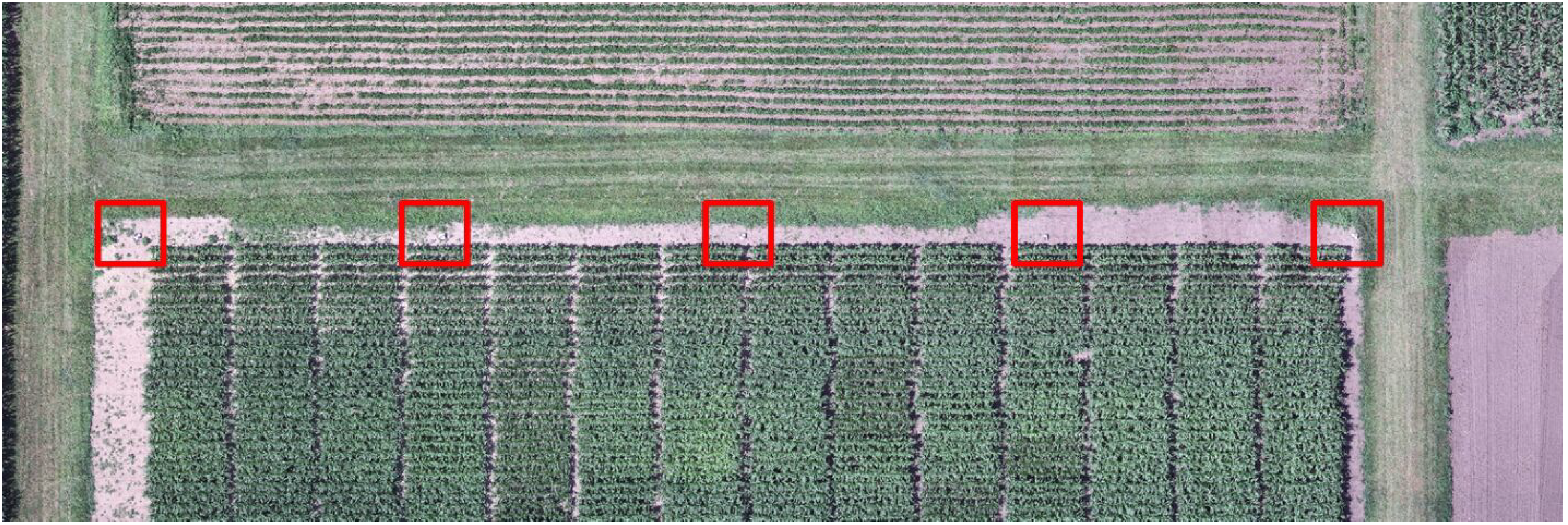
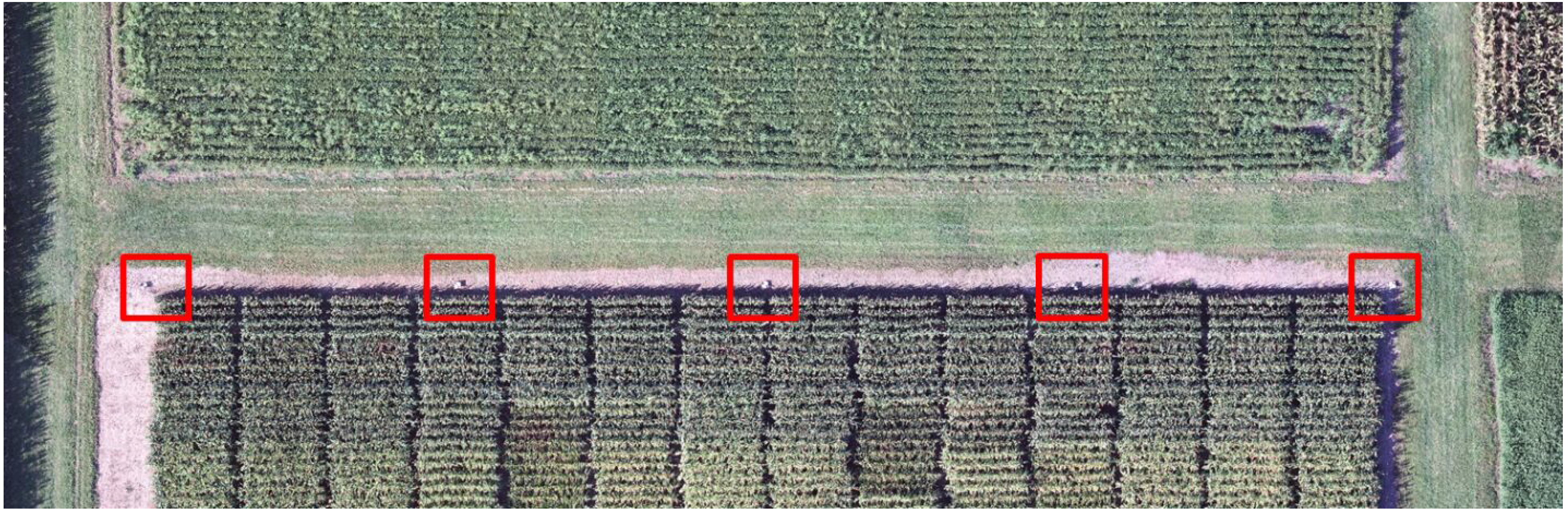
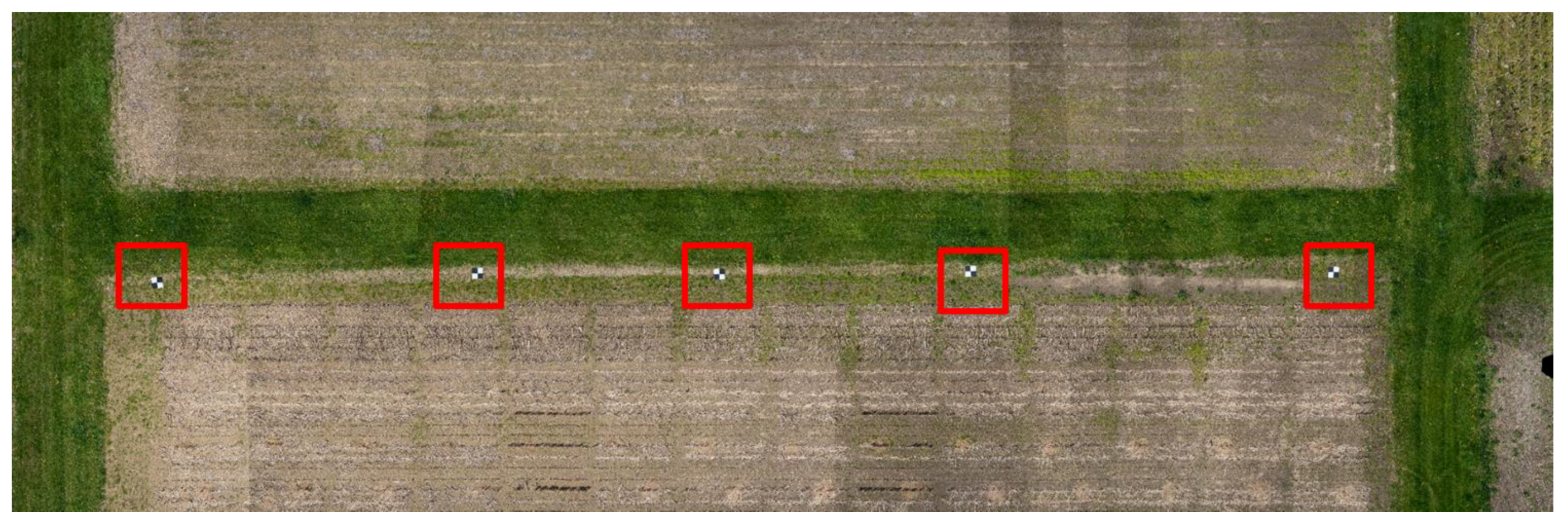
4.1. Data Acquisition

Data for validating the comparative performance of the proposed approaches in this study were acquired using two UAV systems, a Dà-Jiāng Innovations (DJI) Matrice 200 (M200) and a DJI Matrice 600 Pro (M600P) [38,39]. Co-aligned thermal and RGB data were acquired with the DJI M200, and the DJI M600 was used as a second, RGB-only platform. Both systems included an on-board Applanix APX-15 UAV v2 GNSS/INS unit for direct geo-referencing, with a predicted positional accuracy of 2–5 cm and heading and roll/pitch of 0.080 and 0.025°, respectively [40]. Both imaging systems also had the means to send event marker signals to the GNSS/INS unit.

The DJI M200-based imaging system employed a FLIR Duo Pro R 640 combined thermal and RGB image sensor. The Uncooled VOx Microbolometer thermal sensor array was 640 × 512 with a pixel size of 17 μm and had a nominal focal length of 19mm. The RGB visible sensor array size was 4000 × 3000, with a pixel size of 1.85 μm and a nominal focal length of 8 mm [41]. The Duo Pro R has an internal GNSS/INS unit for in-camera geo-tagging, but that unit was not used for this study. Figure 8 shows the FLIR Duo Pro R and APX-15 configuration on the M200 UAV, and illustrates the coordinate systems for the IMU body, camera, and vehicle frames. The FLIR Duo Pro R utilized a mobile-phone based app to set camera parameters via Bluetooth. The mobile-phone based app includes the ability to set the capture interval for the camera and to start and stop triggering. Event feedback to the APX was provided directly by the FLIR Duo Pro R using the “Frame Sync” option. This option output a LVTTL (3.3 V) pulse that was wired directly to the event input of the APX-15. It is important to note that only one triggering interval and frame sync output can be set on the FLIR Duo Pro R, despite the fact that there are two sensors housed in the single unit. Therefore, one might assume that both sensors are capturing images simultaneously. However, during the experiments, the FLIR thermal and RGB sensors were treated independently as separate sensors. The system calibration parameters, including the time delay, were estimated for each senor so the results were not affected by having only one triggering interval.

The second imaging system, flown onboard the DJI M600P, incorporated a Sony Alpha 7R RGB camera and a Velodyne VLP-32C LiDAR sensor, although the LiDAR sensor was not used for this study. The Sony Alpha 7R (ILCE-7R) camera on the DJI M600P had a 7360 × 4912 CMOS array with a 4.9 μm pixel size, and a lens with a nominal focal length of 35 mm [42]. The M600-based RGB-only system used a direct feedback synchronization approach, utilizing the camera flash hot-shoe to generate a signal at the time the image was captured. This camera feedback signal was then sent to the APX-15 and a corresponding event time was recorded. This method also adjusted the event markers during post-processing to account for the constant time delay between the flash operation and the true mid-exposure time [34]. Figure 9 shows the Sony Alpha 7R and APX-15 configuration on the M600.

Table 2. FLIR and Sony nominal boresight angles, lever arm components, and angular field of view.

Sensor	Δω (Degree)	Δφ (Degree)	Δκ (Degree)	Δx (m)	Δy (m)	Δz (m)	Angular FOV (Degrees)
FLIR—Thermal	180	0	−90	0.045	−0.015	0.045	32 × 26
FLIR—RGB				0.045	0.025	0.050	57 × 42
Sony—RGB	180	0	−90	0.260	0.026	−0.010	54 × 38

outlines the nominal boresight and lever arm values, as well as the angular field of view (FOV) for both the FLIR and Sony systems.

4.2. Dataset Description

Five datasets were collected for this time-delay estimation study. Four datasets were collected across two dates, July 25th and September 14th, with the FLIR Duo Pro R. For both collection dates, the FLIR Duo Pro R captured both thermal and RGB images. One RGB dataset from the Sony Alpha 7R camera was also captured and was evaluated alongside the FLIR datasets.

Table 3. FLIR and Sony flight parameters for the different data acquisition dates.

Date	Sensor	Altitude above Ground	Ground Speed	GSD Thermal	GSD RGB	Overlap Thermal/RGB	Sidelap Thermal/RGB	Number of Flight Lines	Number of Images
July 25 2018	FLIR Duo Pro R	20 m	2.7 m/s	1.8 cm	0.7 cm	70/80%	70/80%	6	284
		40 m	5.4 m/s	3.6 cm	1.4 cm	70/80%	70/80%	6	164
Sept. 14 2018		20 m	2.7 m/s	1.8 cm	0.7 cm	70/80%	70/80%	6	294
		40 m	5.4 m/s	3.6 cm	1.4 cm	70/80%	70/80%	6	168
May 05 2019	Sony A7R	20 m	2.7 m/s	-	0.28 cm	70%	82%	6	198
		40 m	5.4 m/s	-	0.56 cm	70%	82%	6	116

outlines the flight and data collection parameters for the FLIR Duo Pro R and the Sony Alpha 7R. All datasets were collected at a research farm. Figure 10 outlines the flight trajectory for both the FLIR and Sony datasets. Figure 11a,b shows the linear and angular velocity variations over the flight time for the July 25th thermal dataset, respectively. Analyzing Figure 11, the change in the linear velocity in the X direction can be explained by the variation in both the flying direction and linear velocity at different flying altitudes. Furthermore, significant changes in the linear and angular velocity were observed in the remaining linear and angular velocity components. This significant change was caused by the small size of the UAV, the impact of the wind, and the attempt of the autopilot to maintain a constant heading. The linear and angular velocities for this data demonstrate that the direct approach uses such variability for reliable estimation of the parameters. The indirect approach, on the other hand, has the capability to tolerate variations which would create decoupling between time delay and lever arm in the along flying direction. All other collection dates had similar linear and angular velocity variations over the flight time.

Five checkerboard targets, used as check points, were deployed in the calibration field for the FLIR and Sony cameras. The ground coordinates of all the checkerboard targets were surveyed by a Topcon GR-5 GNSS receiver with an accuracy of 2–3 cm. The checkerboard targets were identified in raw and orthorectified images to either solve for the unknowns in the GNSS/INS-assisted bundle adjustment with system self-calibration process or check orthorectification accuracy, depending on the method implemented, respectively. Figure 12 shows full-size thermal and RGB imagery captured by the FLIR Duo Pro R camera. Here, it is clear that the angular field of view of the RGB is much larger than that of the thermal. Figure 13 shows the data collection area with enhanced representations of checkerboard targets and a zoomed region of the targets in the thermal and RGB images of the FLIR camera. Figure 14 shows sample RGB imagery captured by the Sony Alpha 7R. Figure 15 shows the flight area of the Sony Alpha 7R calibration field with the five checkerboard targets.

4.3. Experimental Results and Analysis

In this section, the proposed direct and indirect approaches were applied to each dataset, and the experiments tested the validity of the two approaches to successfully estimate time delay in an imaging system. In addition to the direct and indirect approach results, bundle adjustments that ignored the time delay are also presented for further comparison. As described in Section 3.2, the direct approach modifies the mathematical model to include the time delay as a system calibration parameter. This approach was simultaneously applied to both the 20 and 40 m flying height datasets for the DJI M200 and M600 platforms. The indirect approach makes use of existing bundle adjustment software and was applied only to a single flying height: 40 m for the FLIR and Sony cameras. In addition to the direct and indirect approach, bundle adjustment experiments were also conducted while ignoring the time delay, which was also only applied to the 40 m flying height for the FLIR and Sony cameras. The goal of these experiments was to test three main hypotheses. First, that the approaches can be applied to a variety of imaging platforms and maintain the ability to accurately estimate the time delay. Second, that the direct and indirect approaches are comparable. Finally, that the direct and indirect approaches produce consistently accurate results using the original GNSS/INS trajectory file.

Throughout this study, we referred to three different types of point classifications: control, tie, and check points. Control points have known ground points, tie points are interest points used to tie overlapping imagery, and check points are used for numerically evaluating results. Tie points in the indirect approach and in the bundle adjustments that ignored the time delay were established among stereo images using detected features from the Scale Invariant Feature Transform (SIFT) algorithm [43] within a Structure from Motion (SfM) strategy. The SfM algorithm starts with estimating initial relative orientation parameters (ROPs) between overlapping neighboring images while using the position and orientation information provided by the on-board GNSS/INS unit and considering the nominal mounting parameters relating the camera to the GNSS/INS unit. In the next step, SIFT detectors and descriptors are applied to the stereo pairs in question, and potential matches are then identified through a similarity evaluation of the Euclidian distances between SIFT descriptors for the detected features in both images. SIFT-based matches and initial ROPs are used to identify matching outliers based on point-to-epipolar distance of each corresponding point pair. Once all tie points are established among all possible stereo pairs, their ground coordinates are estimated using a simple intersection, and are used later as initial values in the bundle adjustment procedure. These SIFT generated tie points were not used in the direct approach because it can sometimes be difficult to identify automatic tie points in thermal imagery when dealing with data from multiple flying heights. To ensure we could apply the direct approach whether or not automatic tie point detection was used, we used manually measured points that corresponded to signalized targets. Because the direct approach does not use any other tie points except the check points, the direct approach’s results were considered to come from what will be referred to as a mini bundle adjustment. The indirect approach results, as well as the results ignoring the time delay, were considered as a full bundle adjustment.

For all direct approach experiments, the unknown system parameters included lever arm components in the along and across flying directions, boresight angles, time delay, and ground coordinates of check points. It should be noted that the vertical lever arm component was not estimated in any experiments because it would require control points during the adjustments, and these experiments tested the approaches without the use of ground control. In the indirect approach experiments, lever arm components in the along and across flying directions, boresight angles, and ground coordinates of tie points, including check points, were estimated. Once the initial bundle adjustment was performed in the indirect approach, the difference between the nominal and estimated lever arm along the flying direction was computed. Existing time delay was estimated by dividing this difference by the linear velocity, and was then considered to determine the actual time of exposure for each image. Next, IMU body frame position $r_{b\left(t\right)}^m$ and orientation $R_{b\left(t\right)}^m$ was estimated using linear and spherical linear interpolation [44] of available GNSS/INS trajectory data (with 200HZ data rate), respectively. Lastly, a second bundle adjustment was performed with the updated IMU body frame position and orientation to derive the proper lever arm components in the along and across flying directions and boresight angles, as the unknown parameters. The experiments, while ignoring the time delay, used the same IOPs as other experiments, the same check points, and the same SIFT-based tie points. The unknowns consisted of the ground coordinates of the five check points, the ground coordinates of the SIFT-based tie points, and the boresight angles. It should be noted that the lever arm components were intentionally not solved for in the bundle adjustment that ignored time delay, because the time delay error would be absorbed by the lever arm in the along flying direction. For all cameras, IOPs were obtained prior to the experiments. An initial integrated sensor orientation (ISO) bundle adjustment was performed on the FLIR thermal and RBG cameras to obtain the principal distance, principal point coordinates, and distortion parameters. The ISO bundle adjustment used SIFT-based tie points, five GCPs, and GNSS/INS assistance to obtain the IOPs. The IOPs for the Sony RGB camera were estimated through a combination of ISO and an indoor calibration lab procedure. The estimated IOPs were then used throughout all experiments and are presented in

Table 4. Interior orientation parameters (IOPs) for the FLIR and Sony cameras.

Estimated c (Pixel)	Estimated ${\mathit{x}}_{\mathit{p}}$ (Pixel)	Estimated ${\mathit{y}}_{\mathit{p}}$ (Pixel)	Estimated k1 (Pixel-2)	Estimated k2 (Pixel-4)	Estimated p1 (Pixel-1)	Estimated p2 (Pixel-2)
Thermal- FLIR
1131.96	$-5.238$	$3.2$	3.015 × 10−7	9.998 × 10−14	−1.992 × 10−6	2.302 × 10−6
RGB- FLIR
4122.26	$35.07$	$-39.96$	−2.429 × 10−8	−1.250 × 10−15	1.576 × 10−7	−2.693 × 10−7
RGB- Sony
7436.44	$-10.51$	$11.72$	7.771 × 10−10	−6.557 × 10−17	1.906 × 10−7	2.702 × 10−7

.

Qualitative and quantitative analyses are presented for all experiments. The five signalized points were used as check points to numerically evaluate results. The bundle adjustment derived 3D ground coordinates were numerically compared to ground truth data for quantitative analysis. Qualitative analyses were constructed by generating orthophotos with the original trajectory data and visually inspecting for good alignment for both the direct and indirect approaches. Additionally, orthophotos were generated from bundle adjustments while ignoring time delay, both with the original and refined trajectory data, and results were analyzed. The orthophotos were also quantitatively evaluated by measuring check points and numerically comparing them to surveyed ground truth data.

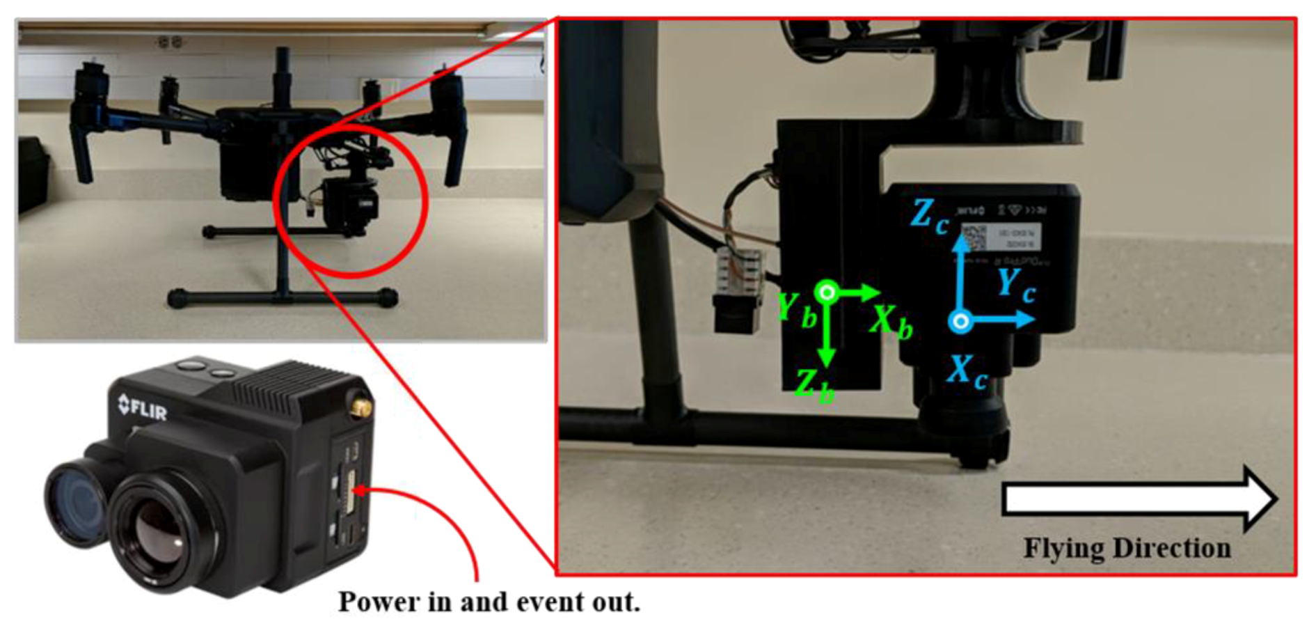
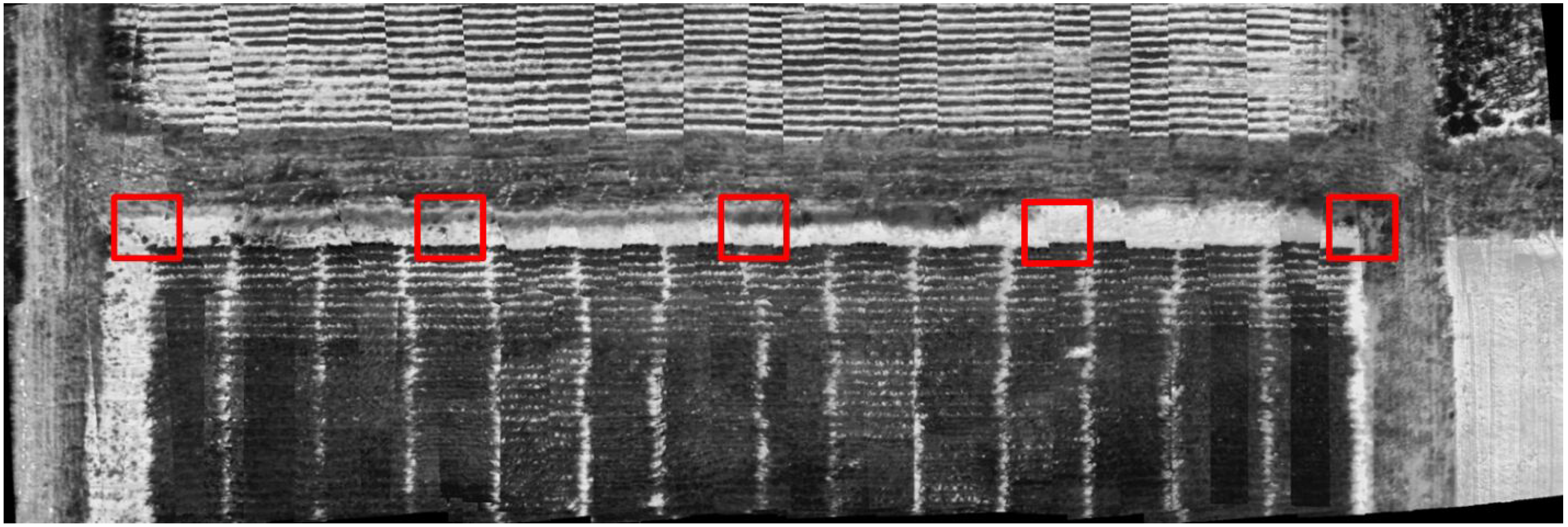
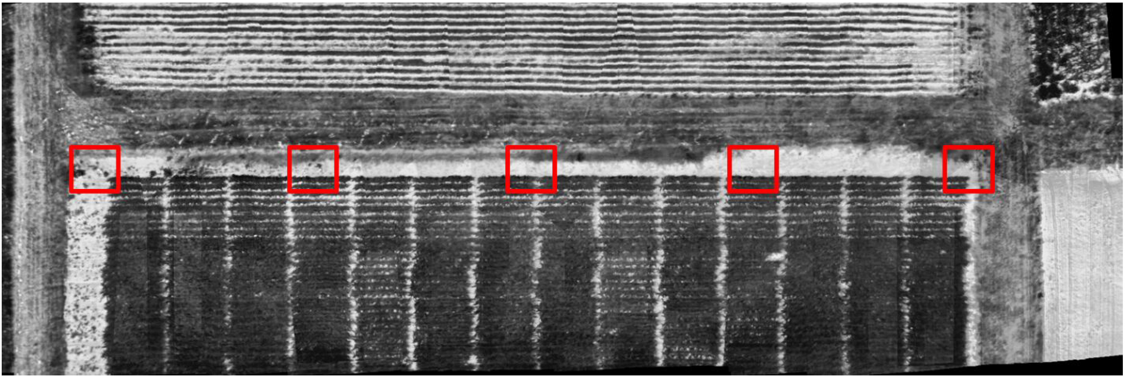
4.3.1. DJI M200 Integrated with FLIR Duo Pro R—FLIR Thermal

A summary of the FLIR thermal sensor results for the direct and indirect approaches while ignoring the time delay is presented in

Table 5. Estimated parameter results for the DJI M200 thermal platform, including the standard deviation for direct results.

	Estimated Time Delay Δt (ms)	Estimated Lever Arm ΔX (m)	Estimated Lever Arm ΔY (m)	Estimated Boresight $\Delta \mathit{\omega }$ (°)	Estimated Boresight $\Delta \mathit{\phi }$ (°)	Estimated Boresight $\Delta \mathit{\kappa }$ (°)	Square Root of A-Posteriori Variance Factor (Pixel) ${\widehat{\mathit{\sigma }}}_{\mathit{o}}$
Ignoring Time Delay (bundle adjustment)
July 25th	NA	NA	NA	179.12	1.26	−90.63	0.67
Sept 14th	NA	NA	NA	179.05	1.23	−90.54	0.84
Direct Approach (mini bundle adjustment)
July 25th	−268 ± 2.6	0.114 ± 0.024	−0.032 ± 0.024	179.03 ± 0.055	−0.395 ± 0.052	−90.82 ± 0.093	4.63
Sept 14th	−261 ± 1.41	0.100 ± 0.015	−0.038 ± 0.014	178.99 ± 0.030	−0.508 ± 0.028	−90.50 ± 0.060	2.19
Indirect Approach (bundle adjustment)
July 25th: Operation 1	N/A	−1.46	−0.015 (constant)	179.11	−0.56	−90.62	0.48
July 25th: Operation 2	−279 *	0.066	−0.29	178.68	−0.56	−90.72	0.47
Sept 14th: Operation 1	N/A	−1.44	−0.015 (constant)	179.05	−0.58	−90.55	0.75
Sept 14th: Operation 2	−275 *	0.142	−0.27	178.68	−0.50	−90.91	0.72

* Time delay was estimated using the difference between the estimated lever arm in flying direction in Operation 1, and its nominal value while considering speed/time/distance relation.

. In Table 5, the boresight angles and the square root of the a-posteriori variance factors are reported for all experiments. The estimated time delay and lever arm components in the across and along flying directions are presented for the direct and indirect approaches. Table 5 shows the estimated boresight Δ$\omega$ and $\Delta \phi$ to be around 180° and −90°, respectively. In the bias impact analysis, we made the assumption that the boresight angles were small. This assumption was only made to simplify the bias impact derivation, and is not a requirement for conducting the estimation process. The time delay was estimated to be −268 and −261 ms for the direct approach on the two collection dates. For the indirect approach, the time delay is estimated to be −279 and −275 ms for the two collection dates. This consistency across the dates allowed estimation of the time delay in an initial system calibration, then use of that estimate for subsequent missions and applications. The square root of the a-posterior variance factor was less than 1 pixel for all experiments except the direct approach. The direct approach had a higher a-posterior variance factor, at 2–4 pixels, because far less tie points were used in the direct approach. The correlation matrix of estimated system parameters for the July 25th direct approach results are reported in

Table 6. Correlation matrix of system parameters for July 25th thermal direct approach results.

	ΔX	ΔY	ΔZ (Not Estimated)	$\Delta \mathit{\omega }$	$\Delta \mathit{\phi }$	$\Delta \mathit{\kappa }$	$\Delta \mathbf{t}$
ΔX	1
ΔY	−0.001	1
ΔZ (not estimated)	0	0	1
Δ$\mathit{\omega }$	0.015	−0.945	0	1
Δ$\mathit{\phi }$	0.885	−0.013	0	0.009	1
Δ$\mathit{\kappa }$	0.011	−0.026	0	0.024	−0.011	1
Δ$t$	−0.023	−0.067	0	0.022	0.326	−0.025	1

. The correlation values were similar in all experiments, therefore only one matrix is displayed in this study. All correlations were low except between the boresight angle $\Delta \phi$ and lever arm component ΔX, as well as between the Δ$\omega$ and ΔY which had correlation values of 0.885 and −0.945, respectively, which are highlighted in red in Table 6. Even though this correlation was high, it would be even higher without using the optimal flight configurations. Tests show that when only one flying height was used for the direct approach, the correlation between the boresight angle $\Delta \phi$ and lever arm component ΔX, as well as between the Δ$\omega$ and ΔY, increased to 0.99. Therefore, using the optimal flight configuration presented in this study decoupled the parameters so that they could be estimated accurately.

Five check points’ 3D coordinates were estimated in all of the experiments.

Table 7. Components and mean/standard deviation/RMSE of the differences between check points and surveyed coordinates for the five check points for the DJI M200 thermal platform.

Without Considering Time Delay Thermal—July				Without Considering Time Delay Thermal—Sept
	${\mathit{X}}_{\mathit{d}\mathit{i}\mathit{f}}\mathbf{\left(}\mathit{m}\mathbf{\right)}$	${\mathit{Y}}_{\mathit{d}\mathit{i}\mathit{f}}\mathbf{\left(}\mathit{m}\mathbf{\right)}$	${\mathit{Z}}_{\mathit{d}\mathit{i}\mathit{f}}\mathbf{\left(}\mathit{m}\mathbf{\right)}$	${\mathit{X}}_{\mathit{d}\mathit{i}\mathit{f}}\mathbf{\left(}\mathit{m}\mathbf{\right)}$	${\mathit{Y}}_{\mathit{d}\mathit{i}\mathit{f}}\mathbf{\left(}\mathit{m}\mathbf{\right)}$	${\mathit{Z}}_{\mathit{d}\mathit{i}\mathit{f}}\mathbf{\left(}\mathit{m}\mathbf{\right)}$
N1	0.03	0.03	−0.18	0.01	−0.05	−0.06
N2	0.05	0.06	−0.29	−0.06	−0.06	−0.12
N3	0.03	0.08	−0.51	−0.03	−0.01	−0.03
N4	−0.04	0.12	−0.12	−0.02	−0.01	0.02
N5	0.04	0.19	0.08	0.070	0.02	0.00
Mean	0.02	0.10	−0.20	−0.01	−0.02	−0.04
Standard Deviation	0.04	0.06	0.22	0.05	0.03	0.05
RMSE	0.04	0.11	0.28	0.05	0.04	0.06
Direct Approach Thermal—July				Direct Approach Thermal—Sept
	${\mathit{X}}_{\mathit{d}\mathit{i}\mathit{f}}\mathbf{\left(}\mathit{m}\mathbf{\right)}$	${\mathit{Y}}_{\mathit{d}\mathit{i}\mathit{f}}\mathbf{\left(}\mathit{m}\mathbf{\right)}$	${\mathit{Z}}_{\mathit{d}\mathit{i}\mathit{f}}\mathbf{\left(}\mathit{m}\mathbf{\right)}$	${\mathit{X}}_{\mathit{d}\mathit{i}\mathit{f}}\mathbf{\left(}\mathit{m}\mathbf{\right)}$	${\mathit{Y}}_{\mathit{d}\mathit{i}\mathit{f}}\mathbf{\left(}\mathit{m}\mathbf{\right)}$	${\mathit{Z}}_{\mathit{d}\mathit{i}\mathit{f}}\mathbf{\left(}\mathit{m}\mathbf{\right)}$
N1	−0.02	0.05	0.14	−0.01	−0.02	0.24
N2	0.01	0.03	0.25	0.01	0.00	0.31
N3	0.01	0.03	0.12	0.00	−0.00	0.27
N4	−0.00	0.03	0.28	0.00	0.01	0.15
N5	−0.04	0.02	0.12	−0.003	0.01	0.16
Mean	−0.01	0.03	0.18	0.00	0.00	0.22
Standard Deviation	0.02	0.01	0.08	0.01	0.01	0.07
RMSE	0.02	0.03	0.19	0.01	0.01	0.23
Indirect Approach Thermal—July				Indirect Approach Thermal—Sept
	${\mathit{X}}_{\mathit{d}\mathit{i}\mathit{f}}\mathbf{\left(}\mathit{m}\mathbf{\right)}$	${\mathit{Y}}_{\mathit{d}\mathit{i}\mathit{f}}\mathbf{\left(}\mathit{m}\mathbf{\right)}$	${\mathit{Z}}_{\mathit{d}\mathit{i}\mathit{f}}\mathbf{\left(}\mathit{m}\mathbf{\right)}$	${\mathit{X}}_{\mathit{d}\mathit{i}\mathit{f}}\mathbf{\left(}\mathit{m}\mathbf{\right)}$	${\mathit{Y}}_{\mathit{d}\mathit{i}\mathit{f}}\mathbf{\left(}\mathit{m}\mathbf{\right)}$	${\mathit{Z}}_{\mathit{d}\mathit{i}\mathit{f}}\mathbf{\left(}\mathit{m}\mathbf{\right)}$
N1	0.01	0.05	−0.11	−0.061	−0.02	0.14
N2	−0.01	0.05	−0.06	−0.078	−0.03	0.12
N3	0.01	0.05	−0.03	−0.03	0.01	0.21
N4	0.00	0.05	0.04	−0.0	−0.00	0.16
N5	0.04	0.07	0.10	0.07	0.01	0.20
Mean	0.01	0.05	−0.01	−0.02	−0.01	0.17
Standard Deviation	0.02	0.01	0.08	0.06	0.02	0.04
RMSE	0.02	0.06	0.07	0.06	0.02	0.17

presents the XYZ components, mean, standard deviation, and RMSE of the differences between check points and surveyed coordinates of the five check points from estimated object point coordinates. As displayed in Table 3, the GSD of the FLIR thermal sensor was in the range of 1.8 to 3.6 cm for the different flying heights. For the direct approach results, the RMSE in the horizontal direction was approximately that of the GSD at 1–3 cm, and the indirect approach results showed no more than two times that of the GSD. Overall, the direct approach produced the best results for the XY components when compared to both the results of the indirect approach, and while ignoring the time delay. The vertical accuracy was much worse than the horizontal one. This was expected and can be explained by the geometric configuration. Using the base height ratio along with the variance in x-parallax, the estimated vertical accuracy was expected to be between 0.09–0.18 m. Therefore, estimated 0.07 and 0.08 m standard deviations in the vertical direction are within reason. Additionally, because of the small test area and the limited number of check points, the Z-component showed a bias, reflected in the mean. For the RMSE Z-component, the indirect approach showed an approximate 26 to 63% decrease from the direct approach. This can be explained by the difference in tie points used. Since the indirect approach used the SIFT-based tie points, there were many more, with better distribution, compared to the few tie points used in the direct approach. That being said, the improvement in the X- and Y-components of the direct approach over the indirect approach and the approach ignoring the time delay shows the superiority of the direct approach. More specifically, even though the direct approach did not use the SIFT-based tie points, which improved point distribution and geometry significantly, the direct approach was still capable of improving the results. The distribution of tie points for the direct and indirect approaches for the Sept 14th FLIR thermal dataset is shown in Figure 16. The distribution of tie points was similar for the other collection dates and sensors in these experiments. Furthermore, the mean standard deviations of the check points are only presented for the direct results, because the bundle adjustments using the large number of SIFT-based tie points did not produce a final dispersion matrix, due to the large size of the unknowns. The mean standard deviation of the five check points derived from the direct approach mini bundle adjustment is displayed in

Table 8. Mean standard deviation of five check points from direct approach for the DJI M200 thermal platform from mini bundle adjustment.

Direct Approach
	X(m)	Y(m)	Z(m)
July 25th	0.018	0.018	0.096
Sept 14th	0.011	0.011	0.072

. Again, the horizontal components had higher accuracy than the vertical.

The above M200 platform—thermal calibration results were used to create 1 cm orthophotos using the estimated system parameters from the results while ignoring the time delay, both using the original and refined trajectory data, as well as the direct and indirect approach results and for all collection dates, using only the original trajectory data. The orthorectification process was carried out by an in-house developed code. An orthophoto resolution of 1 cm was chosen as suitable for the agricultural application requirements. The 40 m flying height images were used for the orthophoto generation. Coordinates of the check targets were then measured on the generated orthophotos. Generating these orthophotos allowed for both a qualitative and quantitative evaluation of the system parameters used for each dataset. Figure 17 shows the orthophoto generated using the system parameters estimated while ignoring the time delay and using the original trajectory data. Figure 18 shows the orthophoto generated using the system parameters estimated while ignoring the time delay, but with the refined trajectory data obtained using the bundle adjustment results. Visually, the orthophoto generated using the refined trajectory data, Figure 18, is much better than that of the one using the original trajectory data, Figure 17. This is because the refined trajectory was obtained from the bundle adjustment results where the exterior orientation parameters (EOPs) absorbed the impact of the time delay i.e., the pitch of the trajectory was modified to absorb the impact of the time delay. Figure 19 and Figure 20 show the orthophotos generated using the direct approach’s calibration results for the July 25th and September 14th collection dates, respectively. The indirect approach’s orthophotos are visually similar to those of the corresponding direct approach results.

Table 9. Derived statistics of horizontal/planimetric coordinate differences for the five check points derived from the orthophoto from the DJI M200 thermal platform.

Ignoring Time Delay—Original Trajectory Data
	Mean—X/Y (m)	Standard Deviation—X/Y (m)	RMSE—X/Y (m)
July 25th	−0.12/−0.07	0.24/0.11	0.25/0.12
Sept 14th	−0.05/−0.12	0.21/0.24	0.23/0.27
Ignoring Time Delay—Refined Trajectory Data
July 25th	−0.02/−0.10	0.03/0.08	0.03/0.13
Sept 14th	0.02/0.02	0.04/0.03	0.05/0.03
Direct Approach—Original Trajectory Data
	Mean—X/Y (m)	Standard Deviation—X/Y (m)	RMSE—X/Y (m)
July 25th	−0.04/−0.07	0.09/0.03	0.10/0.07
Sept 14th	−0.09/0.03	0.14/0.03	0.15/0.03
Indirect Approach—Original Trajectory Data
	Mean—X/Y (m)	Standard Deviation—X/Y (m)	RMSE—X/Y (m)
July 25th	−0.04/−0.07	0.08/0.03	0.08/0.08
Sept 14th	−0.06/−0.06	0.14/0.08	0.14/0.09

shows the statistics of horizontal/planimetric coordinate differences for the five check targets derived from the orthophotos. The results while ignoring time delay but refining the trajectory data prior to generating the orthophoto show comparable results to those of the direct and indirect approaches, which used the original trajectory data, with well-aligned orthophotos and a horizontal accuracy approximately 1–5 times the GSD of the original image. However, refining the trajectory data involves running the bundle adjustment then adjusting the original trajectory data based on the bundle adjustment results for each dataset. The results while ignoring the time delay and using the original trajectory data for generating the orthophoto show accuracy as low as 6–7 times that of the GSD of the original images. The qualitative and quantitative results from the generated orthophotos show that the direct and indirect approach produced accurate results while using the original trajectory data.

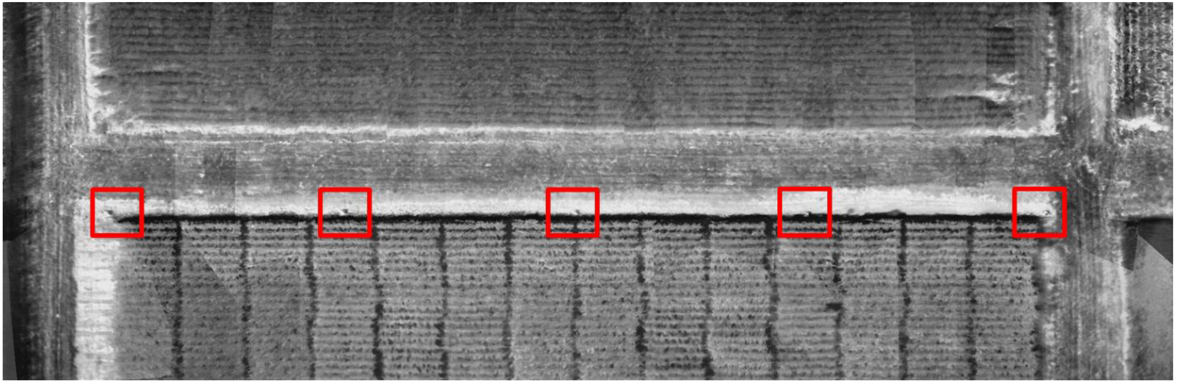
4.3.2. DJI M200 Integrated with FLIR Duo Pro R—FLIR RGB

A summary of the FLIR RGB sensor results for both collection dates, while ignoring the time delay, and for the direct and indirect approaches is presented in

Table 10. Estimated parameter results for the DJI M200 RGB platform including the standard deviation for direct results.

	Estimated Time Delay Δt (ms)	Estimated Lever Arm ΔX (m)	Estimated Lever Arm ΔY (m)	Estimated Boresight $\Delta \mathit{\omega }$ (°)	Estimated Boresight $\Delta \mathit{\phi }$ (°)	Estimated Boresight $\Delta \mathit{\kappa }$ (°)	Square Root of A-Posteriori Variance Factor (Pixel) ${\widehat{\mathit{\sigma }}}_{\mathit{o}}$
Ignoring Time Delay (bundle adjustment)
July 25th	NA	NA	NA	178.55	0.26	−90.84	2.46
Sept 14th	NA	NA	NA	178.61	0.50	−90.67	2.54
Direct Approach (mini bundle adjustment)
July 25th	−205 ± 0.433	0.068 ± 0.005	0.005 ± 0.005	178.57 ± 0.011	0.072 ± 0.011	−90.92 ± 0.014	4.78
Sept 14th	−203 ± 0.457	0.073 ± 0.005	0.0083 ± 0.005	178.58 ± 0.012	0.119 ± 0.011	−90.83 ± 0.015	4.76
Indirect Approach (bundle adjustment)
July 25th: Operation 1	N/A	−0.97	0.025 (constant)	178.56	0.23	−90.87	2.46
July 25th: Operation 2	−188	0.06	−0.02	178.55	0.23	−90.86	2.45
Sept 14th: Operation 1	N/A	−1.03	0.025 (constant)	178.59	0.26	−90.68	2.53
Sept 14th: Operation 2	−199	0.11	−0.03	178.53	0.22	−90.83	2.51

. Table 10 shows the applicable estimated parameters as well as the square root of the a-posterior variance factor for all experiments. Similar to the thermal results, time delay estimated through the two approaches was comparable. Moreover, the two collection dates showed relatively consistent time delay, with time delays estimated to be in the range of −205 and −188 ms for both approaches. Based on the flying speed, the difference in the estimated time delay between −205 and −188 ms equates to approximately 4–9 cm on the ground. Given the APX predicted positional accuracy of 2–5 cm, and heading and roll/pitch of 0.080 and 0.025°, respectively, a difference in results of 4–9 cm on the ground would still be considered consistent results. Having a consistent time delay over multiple collection dates shows the potential to estimate the time delay in a calibration mission and then use that estimate for subsequent missions. However, the time delay estimates from the thermal sensor on the FLIR compared to the RBG sensor showed approximately 60–90 ms difference. This difference shows that the RGB and thermal sensor triggering were not simultaneous, and therefore would need independent calibration adjustments to estimate each sensor’s time delay. The square root of the a-posteriori variance factor was approximately 2.5 pixels for all experiments except the direct approach. The direct approach’s square root of the a-posteriori variance factor was approximately 4.7 pixels. Again, this difference in the a-posterior variance factor was because far fewer tie points were used in the direct approach. The components and the mean/standard deviation/RMSE of the differences between check points and surveyed coordinates for the five check points while ignoring the time delay, as well as for the direct and indirect approaches are presented in

Table 11. Components and mean/standard deviation/RMSE of the differences between check point and surveyed coordinates for the five check points for the DJI M200 RGB platform.

Without Considering Time Delay RGB—July				Without Considering Time Delay RGB—September
	${\mathit{X}}_{\mathit{d}\mathit{i}\mathit{f}}\mathbf{\left(}\mathit{m}\mathbf{\right)}$	${\mathit{Y}}_{\mathit{d}\mathit{i}\mathit{f}}\mathbf{\left(}\mathit{m}\mathbf{\right)}$	${\mathit{Z}}_{\mathit{d}\mathit{i}\mathit{f}}\mathbf{\left(}\mathit{m}\mathbf{\right)}$	${\mathit{X}}_{\mathit{d}\mathit{i}\mathit{f}}\mathbf{\left(}\mathit{m}\mathbf{\right)}$	${\mathit{Y}}_{\mathit{d}\mathit{i}\mathit{f}}\mathbf{\left(}\mathit{m}\mathbf{\right)}$	${\mathit{Z}}_{\mathit{d}\mathit{i}\mathit{f}}\mathbf{\left(}\mathit{m}\mathbf{\right)}$
N1	−0.07	−0.05	0.11	0.06	−0.03	0.07
N2	−0.03	0.01	0.10	0.01	−0.00	0.01
N3	0.01	0.08	0.08	−0.01	−0.03	−0.00
N4	0.04	0.13	0.06	−0.02	0.00	0.08
N5	0.09	0.20	0.01	0.07	0.06	0.14
Mean	0.01	0.07	0.07	0.02	0.00	0.06
Standard Deviation	0.06	0.10	0.04	0.04	0.04	0.06
RMSE	0.06	0.11	0.08	0.04	0.03	0.08
Direct Approach RGB—July				Direct Approach RGB—September
	${\mathit{X}}_{\mathit{d}\mathit{i}\mathit{f}}\mathbf{\left(}\mathit{m}\mathbf{\right)}$	${\mathit{Y}}_{\mathit{d}\mathit{i}\mathit{f}}\mathbf{\left(}\mathit{m}\mathbf{\right)}$	${\mathit{Z}}_{\mathit{d}\mathit{i}\mathit{f}}\mathbf{\left(}\mathit{m}\mathbf{\right)}$	${\mathit{X}}_{\mathit{d}\mathit{i}\mathit{f}}\mathbf{\left(}\mathit{m}\mathbf{\right)}$	${\mathit{Y}}_{\mathit{d}\mathit{i}\mathit{f}}\mathbf{\left(}\mathit{m}\mathbf{\right)}$	${\mathit{Z}}_{\mathit{d}\mathit{i}\mathit{f}}\mathbf{\left(}\mathit{m}\mathbf{\right)}$
N1	0.00	0.04	0.07	−0.00	−0.02	0.10
N2	−0.01	0.03	0.10	−0.01	−0.01	0.11
N3	0.00	0.03	0.12	−0.00	−0.00	0.13
N4	−0.01	0.02	0.12	−0.02	−0.00	0.04
N5	−0.00	0.01	0.09	−0.02	0.00	0.05
Mean	0.00	0.02	0.10	−0.01	−0.01	0.09
Standard Deviation	0.01	0.01	0.02	0.01	0.01	0.04
RMSE	0.01	0.03	0.10	0.01	0.01	0.09
Indirect Approach RGB—July				Indirect Approach RGB—September
	${\mathit{X}}_{\mathit{d}\mathit{i}\mathit{f}}\mathbf{\left(}\mathit{m}\mathbf{\right)}$	${\mathit{Y}}_{\mathit{d}\mathit{i}\mathit{f}}\mathbf{\left(}\mathit{m}\mathbf{\right)}$	${\mathit{Z}}_{\mathit{d}\mathit{i}\mathit{f}}\mathbf{\left(}\mathit{m}\mathbf{\right)}$	${\mathit{X}}_{\mathit{d}\mathit{i}\mathit{f}}\mathbf{\left(}\mathit{m}\mathbf{\right)}$	${\mathit{Y}}_{\mathit{d}\mathit{i}\mathit{f}}\mathbf{\left(}\mathit{m}\mathbf{\right)}$	${\mathit{Z}}_{\mathit{d}\mathit{i}\mathit{f}}\mathbf{\left(}\mathit{m}\mathbf{\right)}$
N1	0.06	0.00	−0.05	−0.05	−0.03	0.05
N2	0.04	0.04	−0.07	−0.05	−0.00	0.01
N3	0.03	0.09	−0.10	−0.03	−0.03	0.08
N4	0.00	0.13	−0.11	−0.04	−0.01	0.14
N5	−0.01	0.17	−0.15	−0.01	0.03	0.18
Mean	0.02	0.04	−0.04	−0.04	−0.01	0.09
Standard Deviation	0.04	0.05	0.03	0.02	0.02	0.07
RMSE	0.04	0.07	0.05	0.04	0.02	0.11

. Again, the horizontal component results for the direct approach were overall improved compared to both the indirect approach and while ignoring the time delay results. The RMSE in the horizontal direction for the direct approach was approximately 1–2 times the GSD of the 40 m flying height imagery. The RMSE in the horizontal direction for the indirect approach and ignoring the time delay was approximately 1–7 times the GSD of the 40 m flying height imagery. The vertical RMSE showed an improvement compared to the thermal sensor at approximately 8–11 cm. This improvement can be explained by the fact that the FLIR RGB has a larger angular FOV, presented in Table 2, which results in a better intersection geometry. Lastly,

Table 12. Mean standard deviation of five check points from direct approach for the DJI M200 RGB platform from mini bundle adjustment.

Direct Approach
	X(m)	Y(m)	Z(m)
July 25th	0.004	0.004	0.015
Sept 14th	0.004	0.004	0.016

shows the mean standard deviation of the five check points for the direct approach obtained in the mini bundle adjustment, with the reported values for the horizontal components being much less than that of the vertical. Again, the mean standard deviations of the check points are only presented for the direct results because the bundle adjustments using the SIFT-based tie points do not produce a final dispersion matrix.

Again, once the calibration was completed the results were then used to generate 1 cm orthophotos while ignoring the time delay, both using the original and adjusted trajectory data, and for the direct and indirect, using the original trajectory data, and using the 40 m flying height data for all collection dates. Figure 21 and Figure 22 show the generated orthophotos for the results while ignoring the time delay. The direct results of the FLIR RGB sensor for both collection dates are shown in Figure 23 and Figure 24. The indirect orthophotos show similar visual results. The results while ignoring the time delay and using the refined trajectory data, as well as the results for the direct and indirect approaches, using the original trajectory data, show well-aligned orthophotos. Using the generated orthophotos, the five check targets were measured and the statistics of the horizontal coordinate differences are shown in

Table 13. Derived statistics of horizontal/planimetric coordinate differences for the five check targets derived from the orthophoto for DJI M200 RGB platform.

Ignoring Time Delay—Original Trajectory Data
	Mean—X/Y (m)	Standard Deviation—X/Y (m)	RMSE—X/Y (m)
July 25th	−1.11/0.06	0.02/0.06	1.12/0.07
Sept 14th	−0.38/−0.05	0.77/0.03	0.78/0.06
Ignoring Time Delay—Refined Trajectory Data
July 25th	−0.01/−0.10	0.07/0.09	0.08/0.13
Sept 14th	−0.01/−0.01	0.05/0.04	0.05/0.04
Direct Approach—Original Trajectory Data
	Mean—X/Y (m)	Standard Deviation—X/Y (m)	RMSE—X/Y (m)
July 25th	−0.04/−0.07	0.06/0.02	0.06/0.07
Sept 14th	0.01/0.01	0.01/0.03	0.01/0.03
Indirect Approach—Original Trajectory Data
	Mean—X/Y (m)	Standard Deviation—X/Y (m)	RMSE—X/Y (m)
July 25th	−0.03/0.07	0.04/0.03	0.05/0.08
Sept 14th	−0.01/0.01	0.03/0.03	0.03/0.03

. These results showed horizontal accuracy ranging from 1–7 times the GSD of the original image. Table 13 shows the direct approach having slightly better results for the evaluation of orthophoto derived points compared to the control data than that of the indirect approach, and ignoring the time delay using the adjusted trajectory data. The results ignoring the time delay and using the original trajectory data were extremely poor and only two of the five check points were visible for measurement.

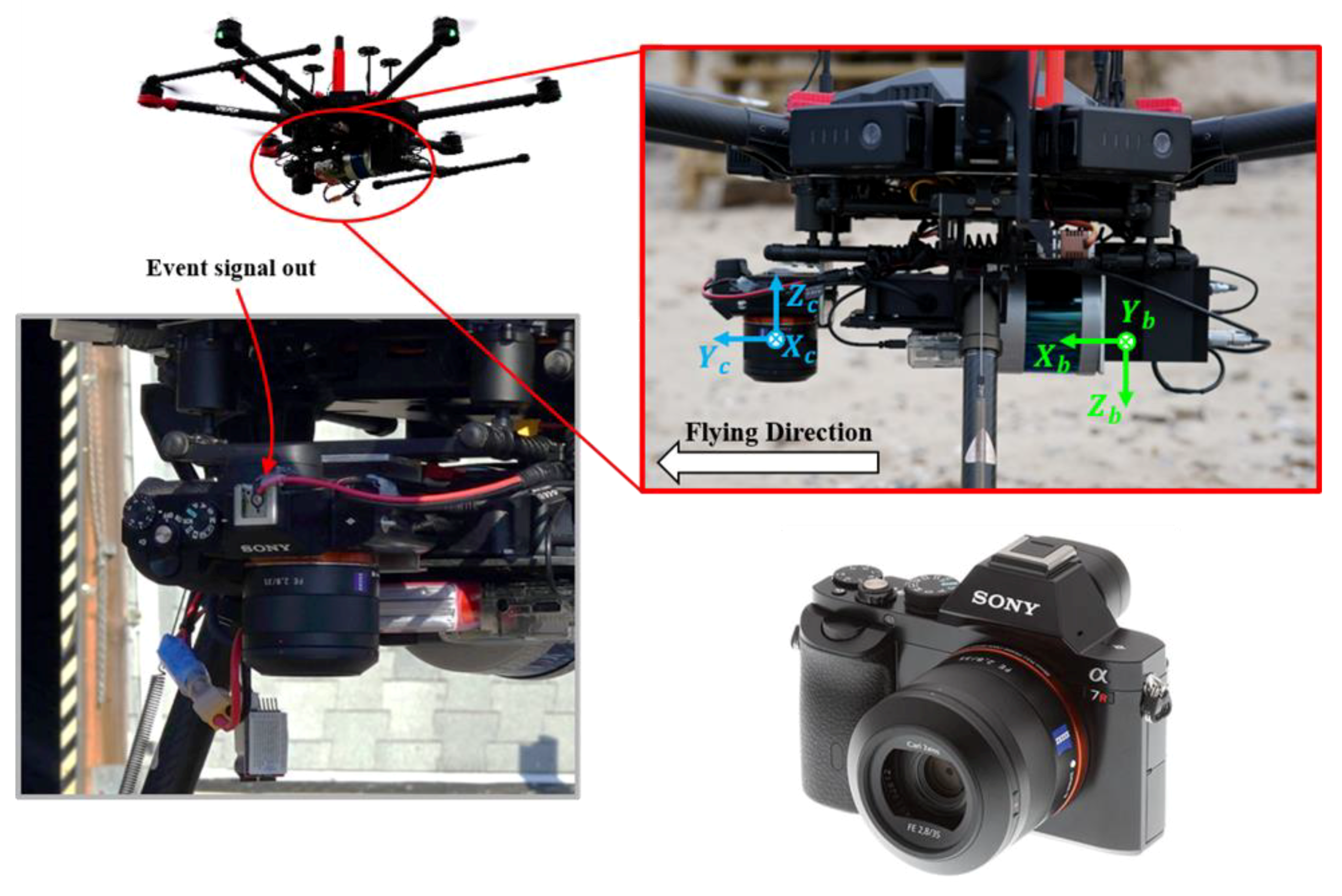
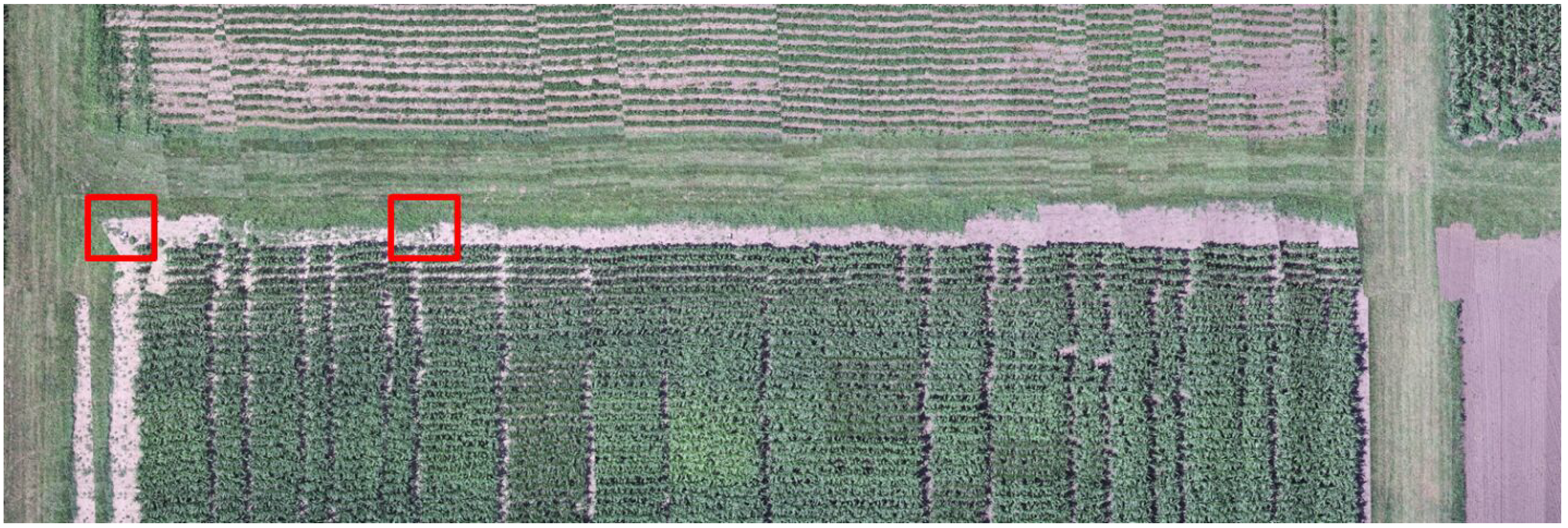
4.3.3. DJI M600 Integrated with Sony Alpha 7R (ILCE-7R)

The results while ignoring the time delay as well as the direct and indirect estimated parameter results for the DJI M600 platform are presented in

Table 14. Estimated parameter results for the DJI M600 platform, including the standard deviations for the direct results.

	Estimated Time Delay Δt (ms)	Estimated Lever Arm ΔX (m)	Estimated Lever Arm ΔY (m)	Estimated Boresight $\Delta \mathit{\omega }$ (°)	Estimated Boresight $\Delta \mathit{\phi }$ (°)	Estimated Boresight $\Delta \mathit{\kappa }$ (°)	Square Root of A-Posteriori Variance Factor (Pixel) ${\widehat{\mathit{\sigma }}}_{\mathit{o}}$
Ignoring Time Delay (bundle adjustment)
May 06th	NA	NA	NA	178.29	−0.09	−91.12	1.56
Direct Approach (mini bundle adjustment)
May 06th	−1.25 ± 0.48	0.267 ± 0.004	0.019 ± 0.004	179.32 ± 0.011	−0.097 ± 0.010	−91.08 ± 0.013	5.61
Indirect Approach (bundle adjustment)
May 06th: Operation 1	N/A	0.268	0.026 (constant)	179.29	−0.09	−91.12	1.56
May 06th: Operation 2	−0.5	0.27	0.002	179.29	−0.09	−91.12	1.56

. It should be noted that this Sony camera was modified prior to collection to incorporate the hardware direct feedback approach [32]. This hardware modification drastically reduced the time delay in the system. As we can see in Table 14, the estimated time delay for the Sony camera was in the range of −1.25 and −0.5 ms for the direct and indirect approaches, respectively. The components, mean, standard deviation, and RMSE of the differences between the check points and surveyed coordinates of the five check points from the bundle adjustment are illustrated in

Table 15. Components and mean/standard deviation/RMSE of the differences between check point and surveyed coordinates for the five check points for the DJI M600 platform—Sony RGB.

Ignoring Time Delay				Direct Approach			Indirect Approach
	${\mathit{X}}_{\mathit{d}\mathit{i}\mathit{f}}\left(\mathit{m}\right)$	${\mathit{Y}}_{\mathit{d}\mathit{i}\mathit{f}}\left(\mathit{m}\right)$	${\mathit{Z}}_{\mathit{d}\mathit{i}\mathit{f}}\left(\mathit{m}\right)$	${\mathit{X}}_{\mathit{d}\mathit{i}\mathit{f}}\left(\mathit{m}\right)$	${\mathit{Y}}_{\mathit{d}\mathit{i}\mathit{f}}\left(\mathit{m}\right)$	${\mathit{Z}}_{\mathit{d}\mathit{i}\mathit{f}}\left(\mathit{m}\right)$	${\mathit{X}}_{\mathit{d}\mathit{i}\mathit{f}}\left(\mathit{m}\right)$	${\mathit{Y}}_{\mathit{d}\mathit{i}\mathit{f}}\left(\mathit{m}\right)$	${\mathit{Z}}_{\mathit{d}\mathit{i}\mathit{f}}\left(\mathit{m}\right)$
N1	−0.04	0.02	−0.00	−0.01	0.02	−0.03	−0.04	0.02	−0.00
N2	−0.03	0.00	−0.05	−0.01	0.01	−0.03	−0.03	0.01	−0.05
N3	−0.03	0.02	−0.06	−0.02	0.02	−0.02	−0.03	0.02	−0.06
N4	−0.01	0.02	−0.07	−0.01	0.01	−0.03	−0.01	0.02	−0.07
N5	0.02	0.01	−0.01	−0.01	−0.00	−0.00	0.02	0.01	−0.01
Mean	−0.02	0.02	−0.04	−0.01	0.01	−0.02	−0.02	0.02	−0.04
Standard Deviation	0.02	0.01	0.03	0.00	0.01	0.01	0.02	0.01	0.03
RMSE	0.03	0.02	0.05	0.01	0.01	0.03	0.03	0.02	0.05

. All results were comparable. This was expected, since the time delay found for this platform was minimal. However, the Δ$\omega$ estimated boresight angle for the direct approach was slightly different than that of the other results. This is because the direct approach did not refine the GNSS/INS data in the adjustment whereas the other bundle adjustments did. Additionally, the a-posterior variance factor was higher for the direct approach. This is because the direct approach only used the check points as tie points in the mini bundle adjustment, compared to the bundle adjustments that used both check points and SIFT-based tie points. The check points had an approximate RMSE of 1–4 and 9 times the GSD for the 40 m flying height, in the horizontal and vertical direction, respectively.

Table 16. Mean standard deviation of five check points from direct approach for the DJI M600 platform from bundle adjustment.

Direct Approach
	X(m)	Y(m)	Z(m)
May 06th	0.003	0.003	0.013

shows the mean standard deviation of the check points from the direct approach mini bundle adjustment. The mean standard deviation for the X, Y, and Z components were very low. The direct approach generated orthophoto from DJI M600 dataset is illustrated in Figure 25, while statistical evaluations of check point targets are presented in

Table 17. Derived statistics of horizontal/planimetric coordinates for five check targets derived from orthophoto—DJI M600 platform.

Ignoring Time Delay—Original Trajectory Data
	Mean—X/Y (m)	Standard Deviation—X/Y (m)	RMSE—X/Y (m)
May 06th	0.03/−0.02	0.02/0.02	0.04/0.03
Ignoring Time Delay—Adjusted Trajectory Data
May 06th	0.02/−0.02	0.02/0.01	0.03/0.02
Direct Approach—Original Trajectory Data
	Mean—X/Y (m)	Standard Deviation—X/Y (m)	RMSE—X/Y (m)
May 06th	0.03/−0.02	0.01/0.02	0.03/0.03
Indirect Approach—Original Trajectory Data
	Mean—X/Y (m)	Standard Deviation—X/Y (m)	RMSE—X/Y (m)
May 06th	0.03/−0.02	0.02/0.02	0.03/0.03

. All other orthophotos generated were visually similar to that of the direct approach, and therefore are not presented. The orthophoto derived coordinates of the check targets showed horizontal RMSE of approximately 2–5 times the GSD in both X and Y directions for the 40 m flying height.

5. Conclusions

UAV-based, GNSS/INS-assisted imaging systems need proper system calibration for accurate 3D spatial reconstruction. With consumer-grade systems, a time delay between the GNSS/INS event markers and the actual exposure time may exist. This time delay needs to be modeled and estimated for accurate geospatial products. In this study, two approaches—direct and indirect—for estimating this time delay are introduced. Optimal flight configuration for system calibration while considering time delay was also derived through bias impact analysis. A modified mathematical model was derived for the direct approach so that the time delay could be directly estimated in a one-step bundle adjustment process. The indirect approach leveraged the traditional mathematical model and bundle adjustment procedure to estimate the time delay indirectly using the nominal lever arm, speed/time/distance relationship, and bias impact analysis findings. Experimental results were presented for two UAV systems with different imaging sensors and multiple collection dates.

In summary, both the direct and indirect approaches accurately estimated the time delay between the GNSS/INS event marker time and the actual image mid-exposure time. The results show that these approaches are capable of producing reliable estimates of the time delay across multiple platforms and with a variety of sensors. The results show that the direct approach is capable of producing accuracy at approximately the same level as the GSD of the system. This accuracy is achieved using direct geo-referencing, without the use of ground control data and while using the original trajectory data. In addition, the results showed consistency across the dates, which allows one to estimate time delay in an initial system calibration, then use that estimate for subsequent missions and applications. The results show that attempting a calibration while ignoring the time delay and using the original trajectory data, for a system with time delay, produces poor orthophoto results both visually and in terms of absolute accuracy evaluation. Ignoring the time delay but adjusting the trajectory did improve results over ignoring the time delay and using the original trajectory. However, adjusting the trajectory information is time consuming and requires an additional bundle adjustment for each dataset. The direct and indirect approaches not only estimated the time delay, but were capable of using the original trajectory data for generating orthophotos. The results also show that the direct and indirect approaches increased the horizontal accuracy compared with the bundle adjustment while ignoring the time delay. Overall, the direct approach is recommended over the indirect because it directly estimates the time delay by modifying the bundle adjustment mathematical model, is capable of incorporating the optimal configuration, and improves absolute accuracy. It is also capable of incorporating multiple flying heights and linear/angular velocities, which allows users to implement the optimal configuration and therefore estimate and decouple system parameters with the highest accuracy. However, both direct and indirect approaches covered in this study can be implemented in system calibration to account for a time delay and used without the need for ground control.

In previous works, there have been both software and hardware solutions for estimating and correcting for time delay in an imaging system. Previous software solutions included either a one-step procedure that required modification to bundle adjustment code, or a two-step procedure that did not require code modification but required two different independent adjustments. All previous software solution studies discussed in this article require ground control points for estimation of the time delay. Furthermore, none of the previous studies presented in this article provided a rigorous derivation of optimal flight configurations. Below is a list of the contributions this study presents:

• Two approaches, direct and indirect, were shown to accurately estimate time delay to accommodate users with and without capability of modifying bundle adjustment software code.
• The indirect approach does not require modification to the bundle adjustment code, and it also only needs a single bundle adjustment process.
• Rigorously derived optimal flight configurations were presented.
• The two approaches were shown to be reliable across a variety of platforms and sensors.
• The direct approach is capable of producing accuracy at approximately the same level as the GSD of the system.
• The accuracies achieved were without the use of ground control points.
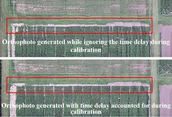
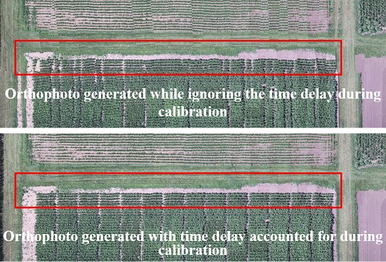
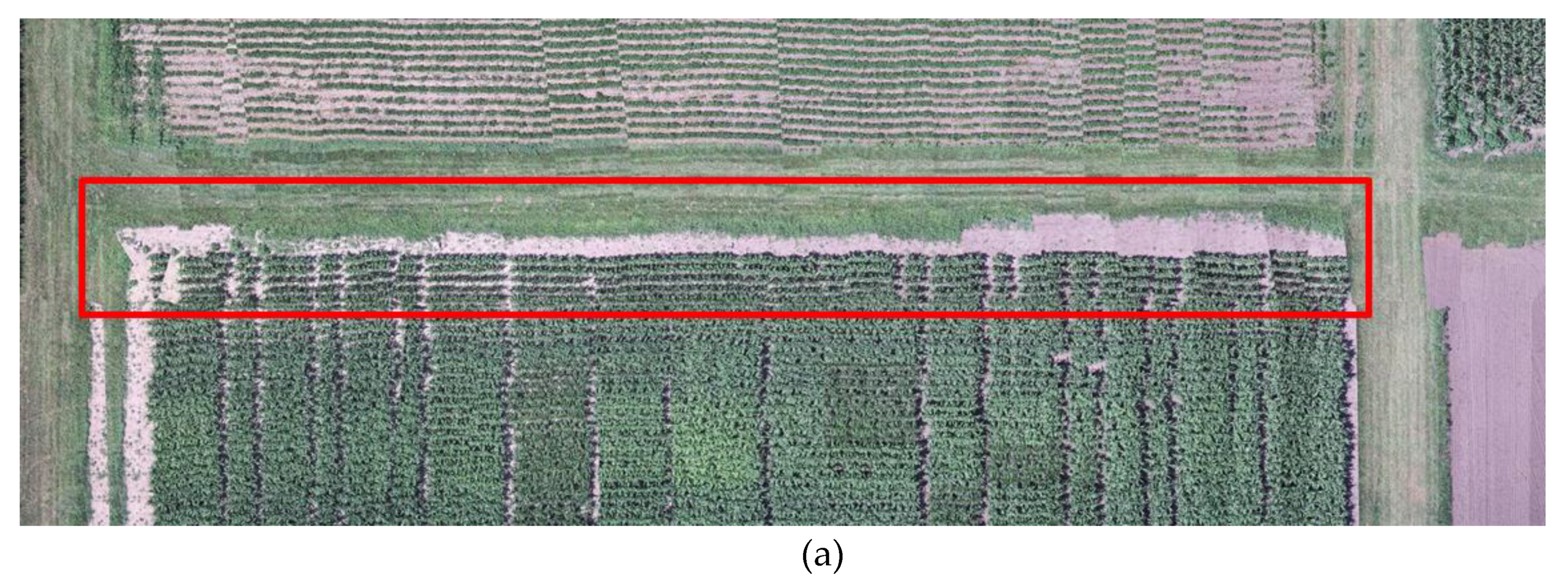
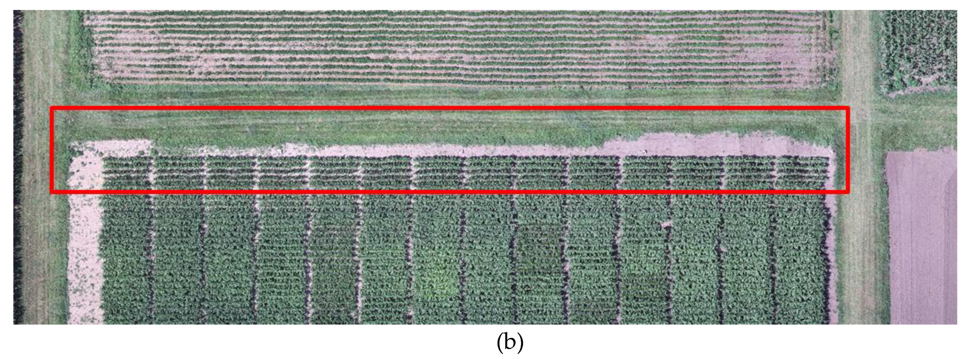
• The direct and indirect approaches are capable of using the original trajectory data for generating accurate orthophotos.
• Both approaches were shown to handle sensors with relatively large time delays appropriately, therefore no prior hardware modification is necessary.

Future work will focus on incorporating the direct approach into a comprehensive bundle adjustment where one could also use SIFT tie points. Automated extraction of targets will also be an avenue of future work. Additionally, an investigation of the internal GNSS/IMU of the FLIR-thermal/RGB sensor will be included to determine whether it also has a time delay. Lastly, using quaternions instead of rotation matrices within the bundle adjustment would allow for better interpolation of platform orientation while considering time delay, and will also be investigated.

References

1. Matese, A.; Toscano, P.; Di Gennaro, S.F.; Genesio, L.; Vaccari, F.P.; Primicerio, J.; Belli, C.; Zaldei, A.; Biancoin, B.; Gioli, B. Intercomparison of UAV, aircraft and satellite remote sensing platforms for precision viticulture. Remote Sens. 2015, 7, 2971–2990. [Google Scholar] [CrossRef]
2. Ravi, R.; Hasheminasab, S.M.; Zhou, T.; Masjedi, A.; Quijano, K.; Flatt, J.E.; Crawford, M.; Habib, A. UAV-based multi-sensor multi-platform integration for high throughput phenotyping. In Autonomous Air and Ground Sensing Systems for Agricultural Optimization and Phenotyping IV; International Society for Optics and Photonics: Baltimore, MD, USA, 2019; Volume 11008, p. 110080E. [Google Scholar]
3. Masjedi, A.; Zhao, J.; Thompson, A.M.; Yang, K.W.; Flatt, J.E.; Crawford, M.; Chapman, S. Sorghum Biomass Prediction Using Uav—Based Remote Sensing Data and Crop Model Simulation. In Proceedings of the IGARSS 2018—2018 IEEE International Geoscience and Remote Sensing Symposium, Valencia, Spain, 22–27 July 2018. [Google Scholar]
4. Zhang, Z.; Masjedi, A.; Zhao, J.; Crawford, M. Prediction of Sorghum biomass based on image based features derived from time series of UAV images. In Proceedings of the 2017 IEEE International Geoscience and Remote Sensing Symposium (IGARSS), Fort Worth, TX, USA, 23–28 July 2017; pp. 6154–6157. [Google Scholar]
5. Chen, Y.; Ribera, J.; Boomsma, C.; Delp, E. Locating crop plant centers from UAV—Based RGB imagery. In Proceedings of the IEEE International Conference on Computer Vision, Venice, Italy, 22–29 October 2017; pp. 2030–2037. [Google Scholar]
6. Buchaillot, M.; Gracia-Romero, A.; Vergara-Diaz, O.; Zaman-Allah, M.A.; Tarekegne, A.; Cairns, J.E.; Prassanna, B.M.; Araus, J.L.; Kefauver, S.C. Evaluating Maize Genotype Performance under Low Nitrogen Conditions Using RGB UAV Phenotyping Techniques. Sensors 2019, 19, 1815. [Google Scholar] [CrossRef] [PubMed]
7. Gracia-Romero, A.; Kefauver, S.C.; Fernandez-Gallego, J.A.; Vergara-Díaz, O.; Nieto-Taladriz, M.T.; Araus, J.L. UAV and Ground Image-Based Phenotyping: A Proof of Concept with Durum Wheat. Remote Sens. 2019, 11, 1244. [Google Scholar] [CrossRef]
8. Pádua, L.; Vanko, J.; Hruška, J.; Adão, T.; Sousa, J.J.; Peres, E.; Morais, R. UAS, sensors, and data processing in agroforestry: A review towards practical applications. Int. J. remote Sens. 2017, 38, 2349–2391. [Google Scholar] [CrossRef]
9. Habib, A.; Han, Y.; Xiong, W.; He, F.; Zhang, Z.; Crawford, M. Automated Ortho-Rectification of UAV—Based Hyperspectral Data over an Agricultural Field Using Frame RGB Imagery. Remote Sens. 2016, 10, 796. [Google Scholar] [CrossRef]
10. Bisquert, M.; Sánchez, J.; López-Urrea, R.; Caselles, V. Estimating high resolution evapotranspiration from disaggregated thermal images. Remote Sens. Environ. 2016, 187, 423–433. [Google Scholar] [CrossRef]
11. Merlin, O.; Chirouze, J.; Olioso, A.; Jarlan, L.; Chehbouni, G.; Boulet, G. An image-based four-source surface energy balance model to estimate crop evapotranspiration from solar reflectance/thermal emission data (SEB-4S). Agric. For. Meteorol. 2014, 184, 188–203. [Google Scholar] [CrossRef] [Green Version]
12. Zhang, D.; Zhou, G. Estimation of Soil Moisture from Optical and Thermal Remote Sensing: A Review. Sensors 2016, 16, 1308. [Google Scholar] [CrossRef]
13. Sun, L.; Schulz, K. The Improvement of Land Cover Classification by Thermal Remote Sensing. Remote Sens. 2015, 7, 8368–8390. [Google Scholar] [CrossRef] [Green Version]
14. Sagan, V.; Maimaitijiang, M.; Sidike, P.; Eblimit, K.; Peterson, K.T.; Hartling, S.; Esposito, F.; Khanal, K.; Newcomb, M.; Pauli, D.; et al. Uav-based high resolution thermal imaging for vegetation monitoring, and plant phenotyping using ici 8640 p, flir vue pro r 640, and thermomap cameras. Remote Sens. 2019, 11, 330. [Google Scholar] [CrossRef]
15. Mikhail, E.M.; Bethel, J.S.; McGlone, J.C. Introduction to Modern Photogrammetry; John Wiley & Sons: New York, NY, USA, 2001; pp. 68–72, 123–125. [Google Scholar]
16. Zhang, Z. A flexible new technique for camera calibration. IEEE Trans. Pattern Anal. Mach. Intell. 2000, 22, 1330–1334. [Google Scholar] [CrossRef]
17. Rathnayaka, P.; Baek, S.; Park, S. Calibration of a Different Field-of-view Stereo Camera System using an Embedded Checkerboard Pattern. In Proceedings of the 12th International Joint Conference on Computer Vision, Imaging and Computer Graphics Theory and Applications, Porto, Portugal, 27 February 2017. [Google Scholar]
18. Habib, A.; Morgan, M.; Lee, Y. Bundle Adjustment with Self-Calibration using Straight Lines. Photogramm. Record 2002, 17, 635–650. [Google Scholar] [CrossRef]
19. Li, Z.; Tan, J.; Liu, H. Rigorous Boresight Self-Calibration of Mobile and UAV LiDAR Scanning Systems by Strip Adjustment. Remote Sens. 2019, 11, 442. [Google Scholar] [CrossRef]
20. Habib, A.; Zhou, T.; Masjedi, A.; Zhang, Z.; Flatt, J.E.; Crawford, M. Boresight Calibration of GNSS/INS-Assisted Push-Broom Hyperspectral Scanners on UAV Platforms. IEEE J. Sel. Top. Appl. Earth Obs. Remote Sens. 2018, 11, 1734–1749. [Google Scholar] [CrossRef]
21. Costa, F.A.L.; Mitishita, E.A. An approach to improve direct sensor orientation using the integration of photogrammetric and lidar datasets. Int. J. Remote Sens. 2019, 1–22. [Google Scholar] [CrossRef]
22. He, F.; Zhou, T.; Xiong, W.; Hasheminnasab, S.M.; Habib, A. Automated Aerial Triangulation for UAV—Based Mapping. Remote Sens. 2018, 10, 1952. [Google Scholar] [CrossRef]
23. Tomaštík, J.; Mokroš, M.; Surový, P.; Grznárová, A.; Merganič, J. UAV RTK/PPK Method—An Optimal Solution for Mapping Inaccessible Forested Areas? Remote Sens. 2019, 11, 721. [Google Scholar] [CrossRef]
24. Chiang, K.; Tsai, M.; Chu, C. The Development of an UAV Borne Direct Georeferenced Photogrammetric Platform for Ground Control Point Free Applications. Sensors 2012, 12, 9161–9180. [Google Scholar] [CrossRef] [Green Version]
25. Padró, J.C.; Muñoz, F.J.; Planas, J.; Pons, X. Comparison of four UAV georeferencing methods for environmental monitoring purposes focusing on the combined use with airborne and satellite remote sensing platforms. Int. J. Appl. Earth Obs. Geoinf. 2019, 75, 130–140. [Google Scholar] [CrossRef]
26. Rehak, M.; Mabillard, R.; Skaloud, J. A Micro-UAV with the Capability of Direct Georeferencing. Int. Arch. Photogramm. Remote Sens. Spat. Inf. Sci. 2013, 40, 317–323. [Google Scholar] [CrossRef]
27. Weng, J.; Cohen, P.; Herniou, M. Camera Calibration with Distortion Models and Accuracy Evaluation. IEEE Trans. Pattern Anal. Mach. Intell. 1992, 14, 965–980. [Google Scholar] [CrossRef]
28. Sedaghat, A.; Mohammadi, N. Illumination-Robust remote sensing image matching based on oriented self-similarity. ISPRS J. Photogramm. Remote Sens. 2019, 153, 21–35. [Google Scholar] [CrossRef]
29. Furukawa, Y.; Ponce, J. Accurate Camera Calibration from Multi-View Stereo and Bundle. Int. J. Comput. Vis. 2009, 84, 257–268. [Google Scholar] [CrossRef]
30. Chiang, K.; Tsai, M.; Naser, E.; Habib, A.; Chu, C. New Calibration Method Using Low Cost MEM IMUs to Verify the Performance of UAV-Borne MMS Payloads. Sensors 2015, 15, 6560–6585. [Google Scholar] [CrossRef] [Green Version]
31. Gabrlik, P.; Cour-Harbo, A.L.; Kalvodova, P.; Zalud, L.; Janata, P. Calibration and accuracy assessment in a direct georeferencing system for UAS photogrammetry. Int. J. Remote Sens. 2018, 39, 4931–4959. [Google Scholar] [CrossRef] [Green Version]
32. Delara, R.; Mitistia, E.A.; Habib, A. Bundle Adjustment of Images from Non-metric CCD Camera Using LiDAR Data as Control Points. In Proceedings of the International Archives of 20th ISPRS Congress, Istanbul, Turkey, 12–23 July 2004. [Google Scholar]
33. Elbahnasawy, M.; Habib, A. GNSS/INS-assisted Multi-camera Mobile Mapping: System Architecture, Modeling, Calibration, and Enhanced Navigation. Ph.D. Thesis, Purdue University, West Lafayette, IN, USA, August 2018. [Google Scholar]
34. Rehak, M.; Skaloud, J. Time synchronization of consumer cameras on Micro Aerial Vehicles. ISPRS J. Photogramm. Remote Sens. 2017, 123, 114–123. [Google Scholar] [CrossRef]
35. Agisoft. 2013. Available online: http://www.agisoft.ru (accessed on 7 June 2019).
36. Blazquez, M. A New Approach to Spatio-Temporal Calibration of Multi-Sensor Systems. In Proceedings of the International Archives of the Photogrammetry, Remote Sensing and Spatial Information Sciences, Beijing, China, 3–13 July 2008. [Google Scholar]
37. Ravi, R.; Lin, Y.; Elbahnasawy, M.; Shamseldin, T.; Habib, A. SimultaneousSystem Calibration of a Multi-LiDAR Multicamera Mobile Mapping Platform. IEEE J. Sel. Top. Appl. Earth Obs. Remote Sens. 2018, 11, 1694–1714. [Google Scholar] [CrossRef]
38. Matrice 200 User Manual. Available online: https://dl.djicdn.com/downloads/M200/20180910/M200_User_Manual_EN.pdf (accessed on 8 November 2018).
39. Matrice 600 Pro User Manual. Available online: https://dl.djicdn.com/downloads/m600%20pro/20180417/Matrice_600_Pro_User_Manual_v1.0_EN.pdf (accessed on 8 November 2018).
40. APX. Trimble APX-15UAV(V2)—Datasheet. 2017. Available online: https://www.applanix.com/downloads/products/specs/APX15_DS_NEW_0408_YW.pdf (accessed on 8 November 2018).
41. FLIR. FLIR Duo Pro R—User Guide. 2018. Available online: https://www.flir.com/globalassets/imported-assets/document/duo-pro-r-user-guide-v1.0.pdf (accessed on 8 November 2018).
42. Sony. Sony ILCE-7R—Specifications and Features. 2018. Available online: https://www.sony.com/electronics/interchangeable-lens-cameras/ilce-7r/specifications (accessed on 8 November 2018).
43. Lowe, D.G. Distinctive Image Features from Scale-Invariant Keypoints. Int. J. Comput. Vis. 2004, 60, 91–110. [Google Scholar] [CrossRef]
44. Shoemake, K. Animating rotation with quaternion curves. ACM SIGGRAPH Comput. Graph. 1985, 19, 245–254. [Google Scholar] [CrossRef]
Figure 1. (a) Orthophoto generated while ignoring the time delay during calibration. (b) Orthophoto generated with time delay accounted for during calibration.
Remotesensing 11 01811 g001aRemotesensing 11 01811 g001b
Figure 2. Conceptual basis of bundle block adjustment.
Remotesensing 11 01811 g002
Figure 3. Illustration of collinearity equations.
Remotesensing 11 01811 g003
Figure 4. Establishing an expression for the correct IMU body frame orientation in the presence of time delay.
Remotesensing 11 01811 g004
Figure 5. Illustration of the direct approach for time delay estimation within the bundle block adjustment with system self-calibration.
Remotesensing 11 01811 g005
Figure 6. Illustration of where measurements are taken to acquire the nominal lever arm values.
Remotesensing 11 01811 g006
Figure 7. Processing workflow of the indirect approach process for time delay estimation.
Remotesensing 11 01811 g007
Figure 8. M200-based thermal/RGB system configuration.
Remotesensing 11 01811 g008
Figure 9. DJI M600-based Sony Alpha 7R system configuration.
Remotesensing 11 01811 g009
Figure 10. Trajectory and target locations for FLIR Duo Pro R and Sony Alpha 7R.
Remotesensing 11 01811 g010
Figure 11. (a) XYZ component linear velocity over flight time for the July 25th thermal dataset. (b) ω ,   φ ,   κ component angular velocity over flight time for the July 25th thermal dataset.
Remotesensing 11 01811 g011
Figure 12. Sample corresponding thermal and RGB images from the FLIR Duo Pro R.
Remotesensing 11 01811 g012
Figure 13. Flight area with enhanced representations of checkerboard targets and sample thermal and RGB images of the FLIR camera around the target location.
Remotesensing 11 01811 g013
Figure 14. Sample images captured by the Sony RBG sensor over the calibration test field. (a) 20 m flying height and (b) 40 m flying height.
Remotesensing 11 01811 g014
Figure 15. Sony A7R calibration field.
Remotesensing 11 01811 g015
Figure 16. Distribution of the tie points used for the FLIR thermal sensor in the Sept. 14th collection date for the direct (right) and indirect* (left) approaches (*only 10% of total tie points are plotted).
Remotesensing 11 01811 g016
Figure 17. Orthophoto result while ignoring the time delay using the original trajectory data for FLIR thermal July 25th data collection (red boxes show the location of the check points, O r i g n a l   I m a g e   G S D 0.03 m ).
Remotesensing 11 01811 g017
Figure 18. Orthophoto result while ignoring the time delay using the refined trajectory data for FLIR thermal July 25th data collection (red boxes show the location of the check points, O r i g n a l   I m a g e   G S D 0.03 m ).
Remotesensing 11 01811 g018
Figure 19. Orthophoto result from direct approach for FLIR thermal July 25th data collection (red boxes show the location of the check points, O r i g n a l   I m a g e   G S D 0.03 m ).
Remotesensing 11 01811 g019
Figure 20. Orthophoto result from direct approach for FLIR thermal September 14th data collection (red boxes show the location of the check points, O r i g n a l   I m a g e   G S D 0.03 m ).
Remotesensing 11 01811 g020
Figure 21. Orthophoto result ignoring the time delay using the original trajectory data for FLIR RGB July 25th data collection (red boxes show the location of the check points—only two visible, O r i g i n a l   I m a g e   G S D 0.01 m ).
Remotesensing 11 01811 g021
Figure 22. Orthophoto result ignoring the time delay using the refined trajectory data for FLIR RGB July 25th data collection (red boxes show the location of the check points, O r i g i n a l   I m a g e   G S D 0.01 m ).
Remotesensing 11 01811 g022
Figure 23. Orthophoto result from direct approach for FLIR RGB July 25th data collection (red boxes show the location of the check points, O r i g i n a l   I m a g e   G S D 0.01 m ).
Remotesensing 11 01811 g023
Figure 24. Orthophoto result from Direct Approach for FLIR RGB September 14th data collection (red boxes show the location of the check points, O r i g i n a l   G S D 0.01 m ).
Remotesensing 11 01811 g024
Figure 25. Orthophoto result from direct approach for Sony—May 06th data collection (red boxes show the location of the check points,   G S D 0.0056 m ).
Remotesensing 11 01811 g025