Random Noise Suppression of Magnetic Resonance Sounding Data with Intensive Sampling Sparse Reconstruction and Kernel Regression Estimation

Abstract

The magnetic resonance sounding (MRS) method is a non-invasive, efficient and advanced geophysical method for groundwater detection. However, the MRS signal received by the coil sensor is extremely susceptible to electromagnetic noise interference. In MRS data processing, random noise suppression of noisy MRS data is an important research aspect. We propose an approach for intensive sampling sparse reconstruction (ISSR) and kernel regression estimation (KRE) to suppress random noise. The approach is based on variable frequency sampling, numerical integration and statistical signal processing combined with kernel regression estimation. In order to realize the approach, we proposed three specific sparse reconstructions, namely rectangular sparse reconstruction, trapezoidal sparse reconstruction and Simpson sparse reconstruction. To solve the distortion of peaks and valleys after sparse reconstruction, we introduced the KRE to deal with the processed data by the ISSR. Further, the simulation and field experiments demonstrate that the ISSR-KRE approach is a feasible and effective way to suppress random noise. Besides, we find that rectangular sparse reconstruction and trapezoidal sparse reconstruction are superior to Simpson sparse reconstruction in terms of noise suppression effect, and sampling frequency is positively correlated with signal-to-noise improvement ratio (SNIR). In one case of field experiment, the standard deviation of noisy MRS data was reduced from 1200.80 nV to 570.01 nV by the ISSR-KRE approach. The proposed approach provides theoretical support for random noise suppression and contributes to the development of MRS instrument with low power consumption and high efficiency. In the future, we will integrate the approach into MRS instrument and attempt to utilize them to eliminate harmonic noise from power line.

1. Introduction

Magnetic resonance sounding (MRS) has attracted much attention in recent years due to accuracy properties of MRS in groundwater detection, which offers important economic benefits. MRS is a relatively efficient and non-invasive geophysical approach for groundwater surveying that utilizes the principle of magnetic resonance phenomenon in hydrogen atoms comprised of water in the geomagnetic field [1,2,3]. The development of nuclear magnetic resonance imaging in the biomedical field has promoted the MRS application in water resources exploration [4,5]. So far, the MRS method and instrument have been further researched and developed in many countries such as France, the United States, Germany, China and other countries [6,7,8]. The MRS method has been applied to hydrological investigation, observation of permafrost thaw, monitoring the cavity in glacier, water-induced disaster detection, and infiltrating water surveys [9,10,11,12,13]. However, when the MRS instrument is exploited for groundwater exploration, the received signal is particularly weak and easily degraded in ambient electromagnetic interference [14]. Furthermore, obtaining the MRS signal with nanovolt-level amplitude is a challenging area in regards to strong electromagnetic noise [15].

Due to noise interference, noise suppression is still a fundamental issue in MRS data processing and there has been extensive research regarding denoising methods in the past decades. The MRS signal is mainly disturbed by three kinds of noise, which are spike noise, harmonic noise and random noise. Spike noise mainly originates from instantaneous discharge, such as lightning, electric fence, and electronic switch. With regard to spike noise suppression, statistical stacking [16] and model-based subtraction [17] are used to deal with it. Harmonic noise mostly stems from power lines and it may seriously damage the MRS signal. In terms of harmonic noise suppression, there are several classical methods, such as bandpass filtering, notch filtering, adaptive notch filter, and model-based elimination method [18]. Nevertheless, notch filtering and adaptive notch filtering may cause the distortion of the phase and amplitude of the MRS signal. The model-based elimination needs to accurately estimate basic frequency of power harmonic noise. In addition, the method of dealing with co-frequency harmonics was studied by Wang et al. [19]. Apart from the interference from spike noise and harmonic noise, the influence of random noise is more common to MRS data. Random noise originates not only from the ambient environment, but also from the internal circuit of the MRS instrument. It is more complex to handle random noise than to cope with harmonic noise and spike noise. If random noise cannot be processed cleanly, it is difficult to obtain an accurate MRS signal. Hence, random noise suppression becomes more and more significant in MRS data processing. For the sake of analyzing the distribution of random noise, Dalgaard et al. developed a noise collector [20]. In order to suppress random noise, a stacking procedure and statistical stacking were used to improve the signal to noise ratio of the MRS signal [16]. Moreover, a global nonlinear least squares parameter fitting scheme was adopted to reduce signal bias amidst strong noise [21], but this scheme demanded synchronization detection which made the control of MRS instrument more complex. In particular, there is another method of eliminating random noise, namely adaptive noise elimination of multichannel MRS instrument [22]. However, this multi-channel noise elimination requires multiple reference coils, which increases the difficulty of field construction. Ghanati et al. proposed a randomized version of the singular value decomposition to accelerate singular spectrum analysis [23]. Besides, time-frequency peak filtering (TFPF) was applied to eliminate random noise of MRS signal [24]. TFPF has achieved good effect in processing random noise, but the signal processed by the method is an envelope of the MRS signal. Although these methods have solved some of the random noise interference in MRS groundwater detection, these methods do not always guarantee to eliminate random noise cleanly. Moreover, there are several denoising methods pertaining to hardware. For examples, the eight shape loop antenna was utilized to overcome high electromagnetic noise [25]. However, the denoising antenna reduces the depth of MRS instrument detection, which is only suitable for shallow groundwater survey. Behroozmand et al. used a central loop method to improve the signal to noise ratio (SNR) of magnetic resonance sounding data [26]. Furthermore, these methods do not involve the random noise elimination associated with sampling aspect.

If performing variable sampling or intensive sampling, then a more accurate signal can be obtained, but intensive sampling generates a lot of data. In data compression, signal and image feature extraction processing of other fields, they provide us some inspiration for processing MRS signals, such as synthetic aperture radar (SAR) images [27], penetrating radar noise filter [28], image processing [29] and so on. In particular, data compression and high-frequency sampling in SAR equipment provide us with exploring direction to process noisy MRS signal. Then, we ponder over the combination of these aspects with MRS data processing and noise suppression. To improve the work efficiency of groundwater detection and reduce the energy consumption of instrument, we propose a novel approach of intensive sampling sparse reconstruction (ISSR) and kernel regression estimation (KRE) to suppress random noise and obtain the MRS full wave signal. Then, to achieve this approach, the ISSR is specifically studied in depth and three sparse reconstructions are proposed and analyzed. We furtherly introduce kernel regression estimation into dealing with the MRS signal processed by the ISSR method. At last, the numerical simulations and field experiments are carried out to verify these methods. One of the outstanding advantages of the research is that suppressing random noise to improve SNR is studied based on a sampling perspective. On the one hand, because the ISSR method reduces the number of stacks by increasing the sampling rate, it provides a theoretical basis for the development of the MRS instrument with low power consumption and high work efficiency. On the other hand, three sparse reconstruction methods provide theoretical guidance and specific methods to suppress random noise by way of variable frequency sampling.

The rest of this paper is structured as follows: Section 2 presents characteristics of MRS signal and classical stacking method. Section 3 illustrates intensive sampling sparse reconstruction and kernel regression estimation approach for suppressing random noise. In Section 4, we conduct numerical simulations in-depth to verify and compare the theoretical denoising effect of the methods in Section 2 and Section 3. In Section 5, we implement field experiments to verify denoising performances of the methods, which are conducted in a magnetic shielding room and in Shaoguo Town, Changchun City, China respectively. In Section 6, we discuss the methods and point out limitations and potential application associated with the approach. In the final section, we provide the conclusions.

2. MRS Signal Analysis and the Classical Stacking Method

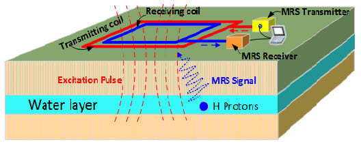
2.1. MRS Signal Analysis

Utilizing the MRS instrument for on-site groundwater detection, the signal collected by the receiver from the receiving coils includes both the MRS signal and electromagnetic noise. To further study noise elimination, it is necessary to understand the generation of MRS signal and the characteristics of the signal. The emission current causes the hydrogen protons in groundwater to jump toward higher energy levels. After the emission current is removed, hydrogen protons relax laterally and decay, and electromagnetic wave with Larmor frequency are radiated outward. Following this, the receiving coil receives the electromagnetic wave containing the MRS signal with Larmor frequency [1,30], as shown in Figure 1.

Neglecting the interference of ambient electromagnetic noise, the MRS full-wave signal $U(t)$ induced in the receiving coil is expressed as Equation (1) [18].

$$U(t)=U_0\cdot e^{(-t/T_2^{*})}\cdot \cos (2\pi f_{Larmor}t+{\phi }_0)$$

(1)

In Equation (1), $f_{Larmor}$ denotes the Larmor frequency, $U_0$, $t$, $T_2^{*}$ and ${\phi }_0$ are the initial amplitude, the recording time, the observed relaxation time and the initial phase respectively. Their units are Hz, nV, ms, ms and degree respectively.

In general, electromagnetic noise is divided into three categories: Spike noise, power frequency harmonic noise and random noise. The focus of this study is the suppression of random noise. Here we use $r(t)$ to represent random noise, then the received noisy signal $S(t)$ is expressed as follows:

$$S(t)=U(t)+r(t)$$

(2)

where the units of $S(t)$, $U(t)$, and $r(t)$ are all nV.

2.2. Classic Stacking Method

In groundwater detection, the MRS signal belongs to the weak signal with nano-volt level. In the implementation of classical stacking method, hydrogen nuclei in groundwater are repeatedly excited by dozens of times, and dozens of data recordings are repeatedly performed at every pulse moment. Then, the collected data is stacked and averaged to achieve signal-to-noise improvement ratio (SNIR) increasing. To comprehend the SNIR concept and to analyze the performance of the method in depth, we present two forms of SNIR (voltage SNIR, power SNIR) of suppressing Gaussian noise according to the literature [31].

$$\{\begin{array}{l}SNI{R}_V=\sqrt{N_S}\\ SNI{R}_p=N_S\end{array}$$

(3)

where $N_S$ represents the number of superposition times in the classic stacking method. Note that if the MRS signal is interfered by Gaussian noise, then the performing stacking of $N_S$ times can make power SNR ($SN{R}_P$) improve by $N_S$ times. That is, the power SNIR ($SNI{R}_P$) is proportional to the stacking number. However, if the noise is non-Gaussian, then the noise suppression effect is reduced by adopting the classic stacking method. In other words, if the noise is other types, then performing stacking of $N_S$ times can make $SN{R}_P$ improve by less than $N_S$ times.

Although classical stacking can suppress the electromagnetic noise interference, there are several shortcomings associated with the method. The control of receiver and transmitter of MRS instrument needs high precision of time synchronization. Due to the multiple currents emitted by the MRS transmitter, the classical stacking method causes low working efficiency and high-power consumption of MRS instrument. The classical stacking method cannot satisfy the demands of fast and mobile detection of MRS technology. In other words, fast and mobile MRS instrument cannot stay too long above a location in groundwater detection.

3. Intensive Sampling Sparse Reconstruction and Kernel Regression Estimation

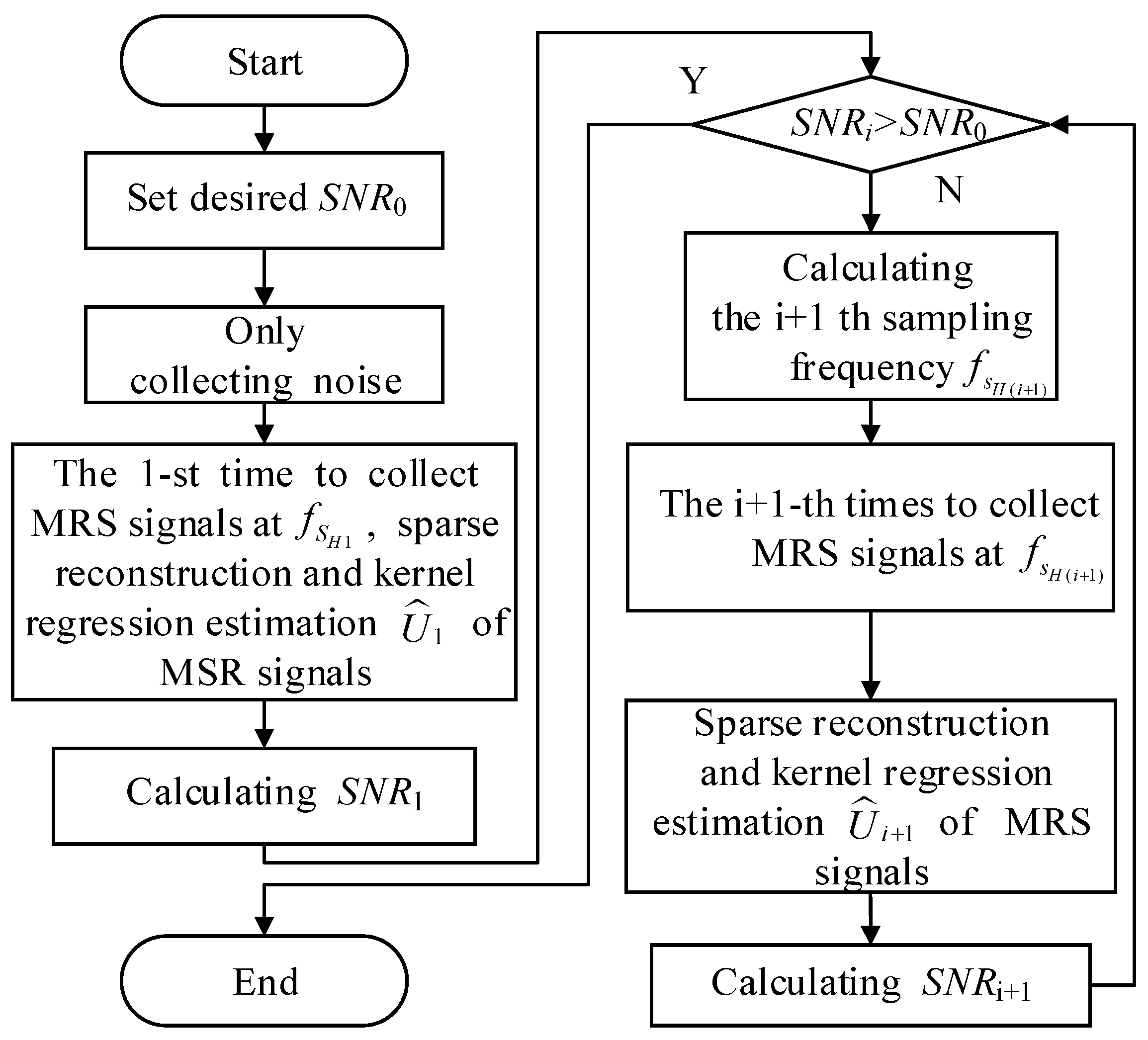
3.1. Overall Approach of ISSR-KRE for Suppressing Random Noise

In order to overcome the deficiencies highlighted in the previous section of classical stacking method, we propose the intensive sampling sparse reconstruction and kernel regression estimation (ISSR-KRE) approach for suppressing random noise. The ISSR-KRE approach includes intensive sampling sparse reconstruction theory and kernel regression estimation theory. This approach only requires one or two excitations for each pulse moment in suppressing random noise. After each emission current is over, intensive sampling of the MRS signal, sparse reconstruction, and kernel regression estimation are performed to achieve random noise suppression.

The basic feature of the ISSR-KRE method is to adopt high sampling frequency $f_{s_H}$ for data acquisition. On the premise that the sampling frequency $f_{s_H}$ satisfies the sampling theorem ($f_{s_H}\ge 2f_c$, $f_c$ represents the highest frequency to measure and its unit is Hz.), if the sampling frequency $f_{s_H}$ is higher, then more points of noisy signal can be obtained.

Although high sampling frequency can obtain plenty of signal information, it also has the disadvantages of containing a large amount of data as well as much more time taken in signal processing. Hence, the ISSR-KRE approach is proposed to achieve small amount of final data and random noise suppression, and the approach is implemented by the steps, as shown in Figure 2. The ISSR-KRE approach mainly consists of the following steps: (i) Setting the desired SNR, (ii) only collecting noise recording, (iii) at the first time, the signal is collected and estimated, (iv) determining to increase the sampling frequency based on the desired SNR, and (v) at the next time, the signal is collected and estimated.

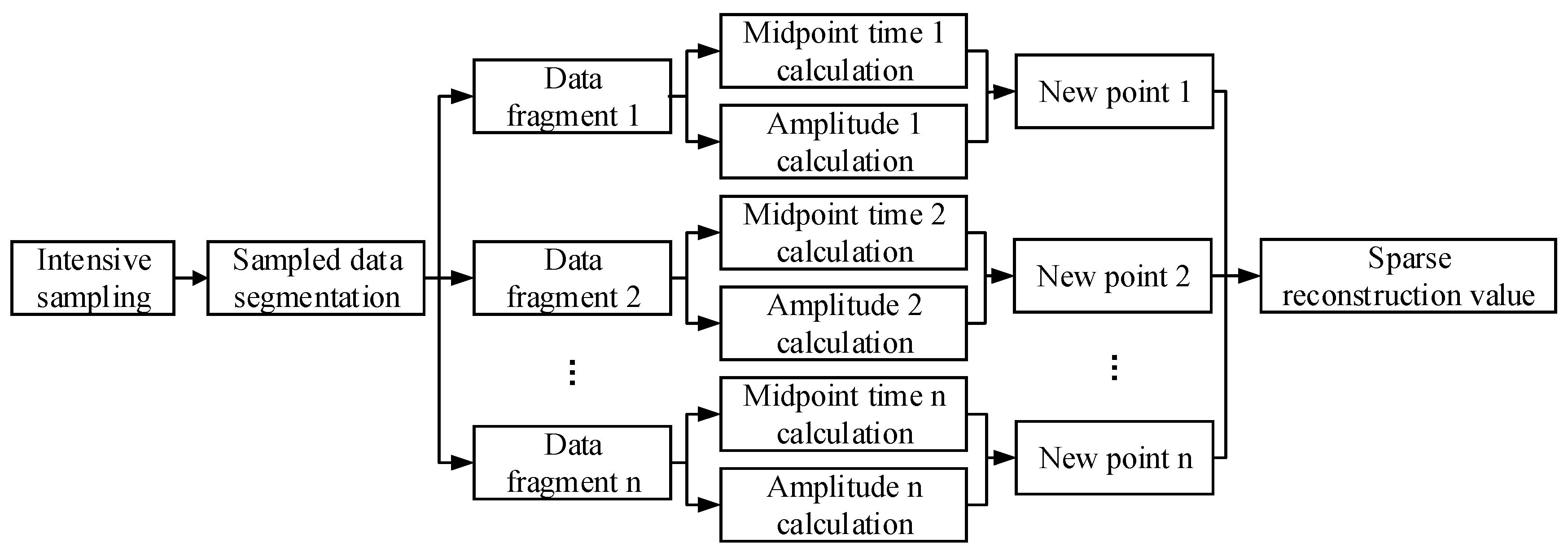
3.2. Intensive Sampling Sparse Reconstruction for Suppressing Random Noise

3.2.1. Basic Frequency of Sparse Reconstruction

In intensive sampling sparse reconstruction, an important operation is to determine the basic frequency $f_{prop}$ of sparse reconstruction. To obtain MRS signal waveform with higher fidelity after ISSR, we define the basic frequency $f_{prop}$, and its unit is Hz. $f_{prop}$ can be understood as the sampling frequency of the reconstructed signal, which satisfies the sampling theorem and is less than $f_{s_H}$, as formula (4).

$$f_{s_H}>f_{prop}>2f_c$$

(4)

According to SNR requirements, $f_{s_H}$ is calculated after determining $f_{prop}$ based on formula (4). In order to prevent the frequency shift of MRS signal after reconstruction, $f_{prop}$ needs further optimization. The optimization of $f_{prop}$ is as shown in Equation (5).

$$f_{prop}=\arg \{g(f_{prop})\in Q\}$$

(5)

where $\arg \{•\}$ is an operator that represents solving the parameters that satisfy the relationship. That is, Equation (5) means finding the parameter $f_{prop}$ that satisfies the relationship $g(f_{prop})\in Q$.

In Equation (5),

$$\{\begin{array}{l}g(f_{prop})=\frac{f_{s_H}}{f_{prop}}\\ Q=\left\{q\right|q=2n+2,n\in N^{*}\}\\ f_{prop}=k{f}_{Larmor}\\ k>2\end{array}$$

(6)

where $g(f_{prop})$ is a function of the argument $f_{prop}$, $Q$ represents a set of integers, $q$ is an element in the set $Q$, $N^{*}$ is the positive integer set, $n$ is an element in the positive integer set $N^{*}$, and $k$ is a real number greater than 2.

After MRS sampling verification, we find that if the sampling rate $f_{s_H}$ is relatively large and if the basic frequency $f_{prop}$ satisfies $f_{prop}\ge 12f_{Larmor}$, the reconstructed signal has higher fidelity. However, $f_{prop}$ cannot be very large. Because $f_{prop}$ is very large to cause a reduction in SNIR and data compression rate.

3.2.2. ISSR Implementation Process

After determining $f_{s_H}$ and $f_{prop}$, the specific steps of ISSR is proposed in Figure 3. The ISSR method mainly includes: (i) Intensive sampling, (ii) sampled data segments, (iii) estimating the time and amplitude of each segment data to form a new reconstructed point, and (iv) sparse reconstructed signal is formed from the new reconstructed points calculated for each segment.

In Figure 3, the used sampling frequency is sampling frequency $f_{s_H}$ with high frequency when performing intensive sampling. The length of each segment is $f_{s_H}/f_{prop}$ in the data segmentation operation. Estimating the time and magnitude of each segmentation data is the core of the ISSR method to form new estimates. In estimating the time and magnitude process, random noise is suppressed and SNR is improved. In addition, another important advantage is that the data is compressed that helps to reduce storage costs and quickly calculate the inversion result of groundwater. In sparse reconstruction, the amount of data can be reduced by $f_{s_H}/f_{prop}$ times. We note that the choice of reconstruction method is directly related to the signal fidelity and SNR improvement of the MRS signal. In the next few sections, we study the specific reconstruction methods to demonstrate their performance. Finally, the reconstructed signal is the signal with a high SNR and a small amount of data.

In order to comprehend intensive sampling of the ISSR method, we give Figure 4. In the figure, $j$ denotes the number of time subinterval, $a$ and $b$ indicate the beginning and end of the time subinterval, respectively. Furthermore, we find that the adjacent sampling interval is very small when performing intensive sampling.

After defining the specific steps of intensive sampling sparse reconstruction, choosing what kind of sparse reconstruction to process each data segment becomes another key issue. To solve this issue, we attempt to employ integration theory. In the mean-value theorem for integrals, if a function $f(x)$ is continuous on $[a,b]$ then there exists $c$ in $[a,b]$ such that: $\frac{1}{b-a}{\displaystyle {\int }_a^{b}f(x)}dx=f(c)$. In other words, we can utilize integral median $f(c)$ instead of $f(x)$ on $[a,b]$. Inspired by this theorem, we explore to adopt a numerical integration method to sparsely reconstruct the signal. In numerical integration, there are three commonly used numerical integration methods: Numerical integration of the rectangular method, numerical integration of the trapezoidal method, and numerical integration of the Simpson method [32]. Moreover, the order of three integration methods, according to integration precision from superior to secondary, is Simpson numerical integration, trapezoidal numerical integration, and rectangular numerical integration.

So far, there are two problems: Whether it is feasible to perform intensive sampling sparse reconstruction of a MRS signal with random noise utilizing these three methods and which method is the best in three methods to suppress random noise. In order to solve the two problems, rectangular sparse reconstruction, trapezoidal sparse reconstruction and Simpson sparse reconstruction are studied respectively. The reason why they are named is so that they are derived based on numerical integration methods. Below we obtain and analyze three methods to process noisy signal with random noise based on SNIR perspective.

3.2.3. Rectangular Sparse Reconstruction

After intensive sampling, the noisy signal is divided into segments with length n per segment where n equals $f_{s_H}/f_{prop}$. Then, according to intensive sampling sparse reconstruction process in Figure 3, we establish the theory of rectangular sparse reconstruction. The details can be found in Appendix A. Further, the specific rectangular sparse reconstruction is selected to process the noisy MRS signal. Importantly, a specific indicator, namely the signal to noise improvement ratio for voltage, is derived for evaluating noise elimination effect of rectangular sparse reconstruction.

$$SNI{R}_{V(\mathrm{Re}\mathrm{ct})}=\frac{SN{R}_{VO}}{SN{R}_{VI}}=\sqrt{\frac{f_{s_H}}{f_{prop}}}$$

(7)

where SNR_VI is SNR for voltage prior to sparse reconstruction, SNR_VO is SNR for voltage after sparse reconstruction, $SNI{R}_{V(\mathrm{Re}\mathrm{ct})}$ denotes signal to noise improvement ratio for voltage of rectangular sparse reconstruction, and the unit of $SNI{R}_{V(\mathrm{Re}\mathrm{ct})}$ is one.

Then SNIR for power is expressed as Equation (8).

$$SNI{R}_{P(\mathrm{Re}\mathrm{ct})}=\frac{f_{s_H}}{f_{prop}}$$

(8)

where, $SNI{R}_{P(\mathrm{Rect})}$ is the signal to noise improvement ratio for power, and the unit of $SNI{R}_{P(\mathrm{Rect})}$ is one.

It can be seen from Equation (8) that $SNI{R}_{P(\mathrm{Re}\mathrm{ct})}$ is proportional to $f_{s_H}$ and inversely proportional to $f_{prop}$. Therefore, SNR can be improved by increasing the sampling frequency $f_{s_H}$ or by selecting a reasonably small $f_{prop}$ to suppress Gaussian random noise.

3.2.4. Trapezoidal Sparse Reconstruction

After intensive sampling, the noisy signal is divided into segments with length n per segment where n equals $f_{s_H}/f_{prop}$. Then, according to intensive sampling sparse reconstruction process in Figure 3, we establish the theory of trapezoidal sparse reconstruction. The details can be found in Appendix A. Further, the specific trapezoidal sparse reconstruction is selected to process the noisy MRS signal. Importantly, a specific indicator, namely signal to noise improvement ratio for voltage SNIR_V, is derived for evaluating noise elimination effect of trapezoidal sparse reconstruction.

$$SNI{R}_{V(\mathrm{Trap})}\approx \frac{2f_{s_H}^{}}{\sqrt{4f_{s_H}{f}_{prop}-2f_{s_H}^2}}$$

(9)

Then SNIR for power is expressed as Equation (10).

$$SNI{R}_{P(\mathrm{Trap})}\approx \frac{2f_{s_H}^2}{2f_{s_H}{f}_{prop}-f_{s_H}^2}$$

(10)

It can be seen from Equation (10) that $SNI{R}_{P(\mathrm{Trap})}$ is positively correlated with $f_{s_H}$ and negatively correlated with $f_{prop}$. Therefore, SNR can be improved by increasing the sampling frequency $f_{s_H}$ or by selecting a reasonably small $f_{prop}$ to suppress Gaussian random noise.

3.2.5. Simpson Sparse Reconstruction

After intensive sampling, the noisy signal is divided into segments with length n per segment where n equals $f_{s_H}/f_{prop}$. Then, according to intensive sampling sparse reconstruction process in Figure 3, we establish the theory of Simpson sparse reconstruction. Appendix A provides the details. Further, the specific Simpson sparse reconstruction is selected to process the noisy MRS signal. Importantly, a specific indicator, namely signal to noise improvement ratio for voltage, is derived for evaluating noise elimination effect of Simpson sparse reconstruction.

$$SNI{R}_{V(\mathrm{Simp})}\approx \frac{3f_{s_H}^{}}{\sqrt{10f_{s_H}{f}_{prop}-2f_{s_H}^2}}$$

(11)

Then SNIR for power is expressed as Equation (12).

$$SNI{R}_{P(\mathrm{Simp})}\approx \frac{9f_{s_H}^2}{10f_{s_H}{f}_{prop}-2f_{s_H}^2}$$

(12)

It can be seen from Equation (12) that $SNI{R}_{P(\mathrm{Simp})}$ is positively correlated with $f_{s_H}$ and negatively correlated with $f_{prop}$. Therefore, SNR can be improved by increasing the sampling frequency $f_{s_H}$ or by selecting a reasonably small $f_{prop}$ to suppress Gaussian random noise.

Ignoring the approximate calculation process influence, comparing the three sparse reconstruction methods according to Equations (8), (10), and (12), we can get: When $f_{s_H}/f_{prop}$ is small, the order of noise suppression effect from superior to secondary is trapezoidal sparse reconstruction, rectangular sparse reconstruction, and Simpson sparse reconstruction. In addition, when $f_{s_H}/f_{prop}$ is large, the noise elimination effect of rectangular sparse reconstruction is close to that of trapezoidal sparse reconstruction, and the noise elimination effect of Simpson sparse reconstruction is the worst. Considering the effect of approximate calculation on the denoising result, the comparison of three sparse reconstructions will be made in the simulation section.

3.3. Kernel Regression Estimation for Suppressing Random Noise

After intensive sampling and sparse reconstruction, there are distortion problems in the peak and valley positions of the signal, and SNR can still be further improved. In order to reduce the signal distortion, one-dimensional kernel regression is used to process the sparse reconstructed signal. The measurement model of one-dimensional signal can be expressed as Equation (13).

$$y_i=f(x_i)+{\epsilon }_i,i=1,2,\cdots ,p$$

(13)

where $y_i$ is the actual measured value of the signal at the i-th sampling point $x_i$, $f(•)$ is the regression function, $x_i$ denotes the time of the i-th sampling point, ${\epsilon }_i$ is the noise value, and $p$ is the number of points participating in the regression calculation.

Although the specific form of $f(x_i)$ is uncertain, we can estimate it by a N-order Taylor series. If x is a point in the field of the sample point x_i, then the Taylor series expansion of the regression function $f(x_i)$ at the time $x$ can be obtained based on Taylor series expansion theory [29].

$$\begin{array}{l}f(x_i)\approx f(x)+f^{\prime }(x)(x_i-x)+\frac{1}{2!}{f}^{″}(x){(x_i-x)}^2+\cdots +\frac{1}{N!}{f}^{(N)}(x){(x_i-x)}^N\\ ={\beta }_0+{\beta }_1(x_i-x)+{\beta }_2{(x_i-x)}^2+\cdots +{\beta }_N{(x_i-x)}^N\end{array}$$

(14)

According to the Taylor series above, if ${\beta }_i$ is known, the regression function $f(x_i)$ can be obtained. In order to minimize the regression error, we utilize the local weighted least squares method to optimize.

$$\underset{\left\{{\beta }_n\right\}}{{\displaystyle \min }}{\displaystyle \sum _{i=1}^P[y_i-{\beta }_0-{\beta }_1(x_i-x)-{\beta }_2{(x_i-x)}^2-\cdots -{\beta }_N{(x_i-x)}^N]}\frac{1}{h}K(\frac{x_i-x}{h})$$

(15)

In Equation (15), $K(•)$ is a kernel function that controls $x_i-x$ weights. $\left|x_i-x\right|$ is smaller, then the weight is larger. $h$ is the smoothing parameter, which affects the penalty strength of $\left|x_i-x\right|$. When the smoothing factor h is larger, the regression curve of the signal becomes smoother; otherwise the regression curve is not smooth. The form of $K(•)$ is not unique as long as the following conditions are met:

$${\displaystyle \underset{R^1}{\int }\tau K(\tau )}d\tau =0,{\displaystyle \underset{R^1}{\int }{\tau }^{2}K(\tau )}d\tau =c$$

(16)

where c is a constant. Common kernel functions include linear kernel function, Gaussian kernel function, and polynomial kernel function. Since the choice of kernel has little influence on the estimation accuracy, this paper chooses Gaussian kernel function to estimate the signal processed by sparse reconstruction. The Gaussian kernel function is as follows.

$$K_h(\tau )=\frac{1}{h}\cdot \frac{1}{\sqrt{2\pi }}\cdot e^{-\frac{1}{2}{(\frac{\tau }{h})}^2}$$

(17)

where $\tau$ means $x_i-x$. For the selection of different orders N, local estimation of noisy signal can be achieved. In nonparametric statistical theory, N=0, 1, 2 is widely used.

(i) When $N=0$, the famous Nadaraya-Watson estimate (NWE) is obtained, and its form is as shown in Equation (18). NWE is a local constant estimator.

$$\widehat{f}(x_i)={\beta }_0=\frac{{\displaystyle \sum _{i=1}^P{K}_h(x_i-x)y_i}}{{\displaystyle \sum _{i=1}^P{K}_h(x_i-x)}},K_h(\tau )=\frac{1}{h}K(\frac{\tau }{h})$$

(18)

(ii) When $N=1$, we can get a local linear kernel regression estimator.

$$\widehat{f}(x_i)=X_1{A}^{-1}B$$

(19)

where $X_1=[\begin{array}{cc}1& x_i\end{array}-x]$, $A=\left[\begin{array}{cc}{\displaystyle \sum _{i=1}^P{K}_h(x_i-x)}& {\displaystyle \sum _{i=1}^P(x_i-x)K_h(x_i-x)}\\ {\displaystyle \sum _{i=1}^P(x_i-x)K_h(x_i-x)}& {\displaystyle \sum _{i=1}^P{(x_i-x)}^2{K}_h(x_i-x)}\end{array}\right]$, $B=\left[\begin{array}{c}{\displaystyle \sum _{i=1}^P{y}_i{K}_h(x_i-x)}\\ {\displaystyle \sum _{i=1}^P(x_i-x)y_i{K}_h(x_i-x)}\end{array}\right]$.

(iii) When $N=2$, we can get a local quadratic kernel regression estimator.

$$\widehat{f}(x_i)=X_2{A}^{-1}B$$

(20)

where $X_2=[{\begin{array}{ccc}1& x_i-x& (x_i-x)\end{array}}^2]$, $A=\left[\begin{array}{ccc}{\displaystyle \sum _{i=1}^P{K}_h(x_i-x)}& {\displaystyle \sum _{i=1}^P(x_i-x)K_h(x_i-x)}& {\displaystyle \sum _{i=1}^P{(x_i-x)}^2{K}_h(x_i-x)}\\ {\displaystyle \sum _{i=1}^P(x_i-x)K_h(x_i-x)}& {\displaystyle \sum _{i=1}^P{(x_i-x)}^2{K}_h(x_i-x)}& {\displaystyle \sum _{i=1}^P{(x_i-x)}^3{K}_h(x_i-x)}\\ {\displaystyle \sum _{i=1}^P{(x_i-x)}^2{K}_h(x_i-x)}& {\displaystyle \sum _{i=1}^P{(x_i-x)}^3{K}_h(x_i-x)}& {\displaystyle \sum _{i=1}^P{(x_i-x)}^4{K}_h(x_i-x)}\end{array}\right]$, $B=\left[\begin{array}{c}{\displaystyle \sum _{i=1}^P{y}_i{K}_h(x_i-x)}\\ \begin{array}{l}{\displaystyle \sum _{i=1}^P(x_i-x)y_i{K}_h(x_i-x)}\\ {\displaystyle \sum _{i=1}^P{(x_i-x)}^2{y}_i{K}_h(x_i-x)}\end{array}\end{array}\right]$.

In general, N is positively correlated with the variance of estimated values and N is negatively correlated with the deviation of estimated values.

4. Numerical Simulations

The method proposed in this paper will be verified by simulation experiments and field experiments. In order to clearly compare the noise suppression in the experiments, the SNR for power, the mean squared error (MSE) and the SNIR for power (Equations (8), (10) and (12)) are utilized as indicators for evaluating the method effectiveness. SNR and MSE are defined as follows:

$$SNR=10{\log }_{10}(\frac{P_U}{P_r})=10{\log }_{10}(\frac{{\displaystyle \sum _{i=1}^N{U}_i^2}}{{\displaystyle \sum _{i=1}^N{r}_i^2}})$$

(21)

where $P_U$ and $P_r$ represent the signal power and the noise power, respectively; $U_i$ and $r_i$ represent the signal voltage and the noise voltage, respectively. The unit of SNR for power is dB.

$$MSE=\frac{{\displaystyle \sum _{i=1}^N{[S_i-U_i]}^2}}{N}$$

(22)

where $S_i$ denotes the noisy signal voltage, $N$ is the total number of discrete signal points. The unit of MSE is nV².

It can be seen from Equation (21) and Equation (22) that the larger the SNR is, the smaller the MSE is. Then, $S(t)$ is closer to $U(t)$, and the noise reduction effect becomes better.

4.1. Simulations of Intensive Sampling Sparse Reconstruction for Random Noise Suppression

4.1.1. Sparse Reconstruction Simulation

In the simulation experiment, the acquisition time length is 250 ms, and the initial amplitude of the MRS signal $U_0$ = 40.46 nV, the Larmor frequency $f_{Larmor}$ = 2341.7 Hz, $T_2^{*}$ = 500 ms. The synthesized noisy signal is composed of MRS signal and Gauss white noise. When synthesizing a noisy MRS signal, random noise is determined to be added into MRS signal based on the value of signal-to-noise ratio. In simulation, the initial SNR of synthetic noisy signal is −20 dB.

In Figure 5, the left-hand column is the time-series. The blue lines display the time-series of the sampling frequency $f_{prop}$. The red lines display the time-series of rectangular sparse reconstruction by different sampling frequencies. The right-hand column is the spectra. The blue lines display the spectra of the time-series of the sampling frequency $f_{prop}$, and the red lines display the spectra of the time-series of rectangular sparse reconstruction by different sampling frequencies that correspond to the left-hand column.

According to determining the basic frequency method in Section 3.2.1, firstly setting $f_{prop}$ > 12$f_{Larmor}$, we calculate the solutions of $f_{prop}$ by Equation (5) and Equation (6), then we choose the solution $f_{prop}$ = 24$f_{Larmor}$. Following this, we adopt the sampling frequency $f_{s_H}$ = 8$f_{prop}$, 16$f_{prop}$, 32$f_{prop}$, 64$f_{prop}$ to intensively sample the noisy MRS signal and to restructure the noisy signal by way of rectangular sparse reconstruction. After rectangular sparse reconstruction, the SNR of the restructured signal is –10.9537 dB, –7.8869 dB, –4.9097 dB, –1.9680 dB and SNIR is 7.7996, 15.8032, 31.3668, 61.7511, respectively. The time domain waveform and the frequency domain amplitude of the reconstructed signals are shown in Figure 5.

The curves in Figure 6 are statistically obtained from 20 experimental simulations. In each simulation, the SNR of synthesized noisy signal is −20 dB. In Figure 6, the first row shows the curves of power signal to noise ratio by logarithmic representation and the curves of power signal-to-noise ratio by non-logarithmic representation, respectively. The unit of SNR by logarithmic representation is dB. The unit of SNR by non-logarithmic representation is 1. The second row shows the curves of SNIR for power and MSE, respectively. The unit of SNIR for power is 1. The unit of MSE is nV². The blue lines display simulation experimental value, and the red lines display the theoretical value.

From Figure 6, SNR and SNIR are proportional to the sampling frequency $f_{s_H}$ when $f_{prop}$ is constant. MSE is inversely proportional to $f_{s_H}$. The experiments show that the sparse reconstruction of rectangular method is feasible to suppress random noise, and Equations (7) and (8) are verified.

In addition, the simulation processes of trapezoidal sparse reconstruction and Simpson sparse reconstruction are similar to simulation process of rectangular sparse reconstruction. Here we only give simulation results of trapezoidal sparse reconstruction and Simpson sparse reconstruction.

In trapezoidal sparse reconstruction, when the basic frequency $f_{prop}$ is constant, SNR and SNIR are positively related to the sampling frequency $f_{s_H}$ and MSE is negatively related to the sampling frequency $f_{s_H}$. The experiments show that trapezoidal sparse reconstruction is feasible to suppress random noise, and Equations (9) and (10) are verified.

In Simpson sparse reconstruction, when the basic frequency $f_{prop}$ is constant, SNR and SNIR are positively related to the sampling frequency $f_{s_H}$ and MSE is negatively related to the sampling frequency $f_{s_H}$. The experiments show that the sparse reconstruction of Simpson method is feasible to suppress random noise, and Equations (11) and (12) are verified.

4.1.2. Comparison of Three Sparse Reconstructions

This sub-section compares rectangular sparse reconstruction, trapezoidal sparse reconstruction and Simpson sparse reconstruction, and then we analyze the advantages and disadvantages of three sparse reconstructions. The comparison indicators include SNR, SNIR, MSE, and waveform.

In this simulation experiment, we see that the initial amplitude of noiseless MRS signal, the Larmor frequency, the observed relaxation time and the length of recording time are equal to 40.46 nV, 2341.7 Hz, 500 ms and 250 ms respectively. The SNR of synthesized noisy signal is −20 dB. The same collected data is processed by three different sparse reconstructions, and the indicators are compared.

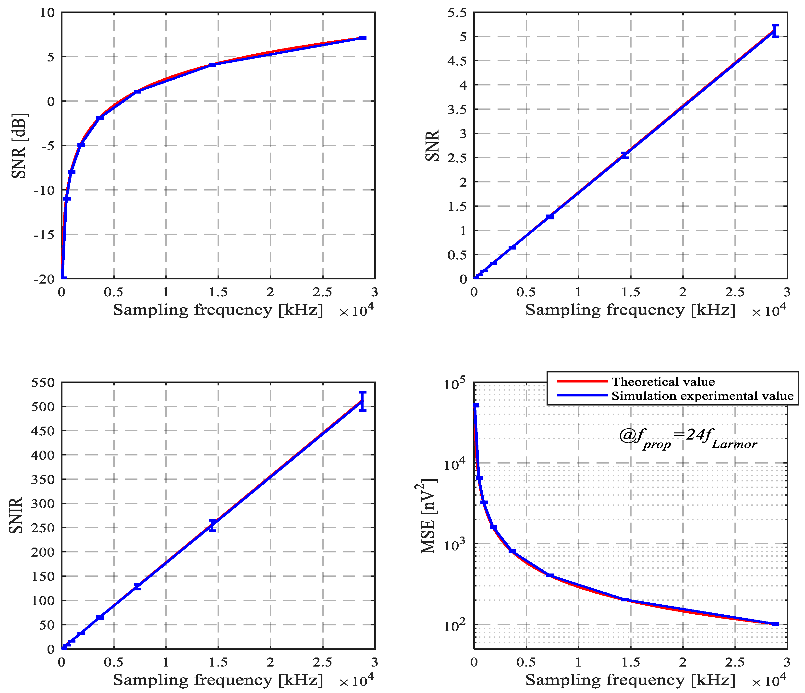
Comparison of SNR, SNIR and MSE

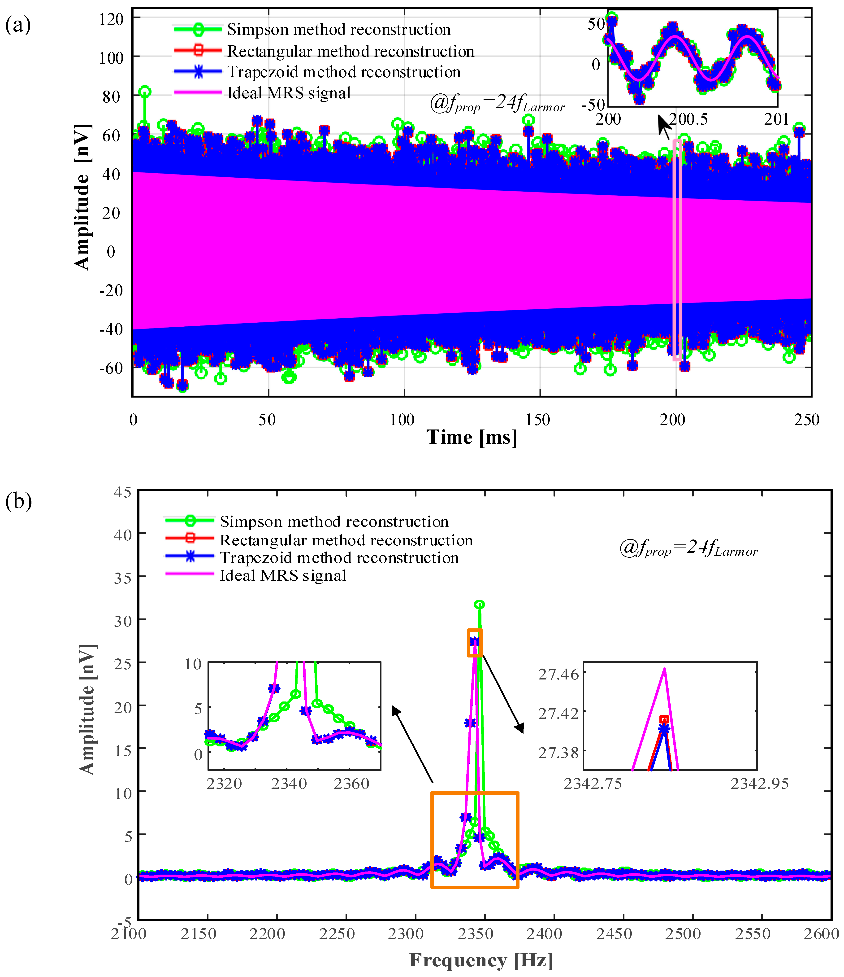
In Figure 7, we compare the performance of three sparse reconstruction methods (namely (rectangular sparse reconstruction, trapezoidal sparse reconstruction and Simpson sparse reconstruction). Figure 7a is comparison of signal-to-noise ratio of noisy MRS signal processed by the three methods. It can be seen from the figure that the signal-to-noise ratio of the noisy MRS signal processed by rectangular sparse reconstruction is better than that by other two kinds of sparse reconstruction. Figure 7b is a comparison of the signal-to-noise improvement ratio of a noisy MRS signal processed by three methods. We can find that the signal-to-noise improvement ratio of the noisy MRS signal processed by the rectangular sparse reconstruction is the best. Figure 7c is a comparison of the mean squared error of the noisy MRS signal processed by three methods. It can be seen that the MSE value of the noisy MRS signal processed by Simpson sparse reconstruction is larger than that by rectangular sparse reconstruction and trapezoidal sparse reconstruction.

In

Table 1. SNR comparison of three ISSR methods in the experiment. The estimated parameters, $SN{R}_{\mathrm{Re}ct}$, $SN{R}_{Trap}$ and $SN{R}_{Simp}$ are reported based on the synthetic MRS signal with $U_0^{}$ = 40.46 nV, $T_2^{*}$ = 500 ms, $f_{Lamor}$ = 2341.7 Hz, $f_{prop}$ = 24$f_{Lamor}$ and initial SNR = −20 dB.

${\mathit{f}}_{{\mathit{s}}_{\mathit{H}}}(\mathbf{Hz})$	$\mathbf{8}{\mathit{f}}_{\mathit{p}\mathit{r}\mathit{o}\mathit{p}}$	$\mathbf{16}{\mathit{f}}_{\mathit{p}\mathit{r}\mathit{o}\mathit{p}}$	$\mathbf{32}{\mathit{f}}_{\mathit{p}\mathit{r}\mathit{o}\mathit{p}}$	$\mathbf{64}{\mathit{f}}_{\mathit{p}\mathit{r}\mathit{o}\mathit{p}}$	$\mathbf{128}{\mathit{f}}_{\mathit{p}\mathit{r}\mathit{o}\mathit{p}}$	$\mathbf{256}{\mathit{f}}_{\mathit{p}\mathit{r}\mathit{o}\mathit{p}}$	$\mathbf{512}{\mathit{f}}_{\mathit{p}\mathit{r}\mathit{o}\mathit{p}}$
$SN{R}_{\mathrm{Re}ct}-SN{R}_{Trap}(dB)$	0.2519	0.0999	0.0610	0.0487	0.0253	0.0032	0.0027
$SN{R}_{\mathrm{Re}ct}-SN{R}_{Simp}(dB)$	0.3419	0.3650	0.3974	0.4625	0.4689	0.4814	0.4970

, $SN{R}_{\mathrm{Re}ct}$, $SN{R}_{Trap}$ and $SN{R}_{Simp}$ represent the SNR of rectangular sparse reconstruction, trapezoidal sparse reconstruction and Simpson sparse reconstruction, respectively. According to Figure 7 and Table 1, we can conclude that, in this case of strong noise, the order of three sparse reconstructions in the light of denoising effect from superior to secondary is rectangular sparse reconstruction, trapezoidal sparse reconstruction, and Simpson sparse reconstruction. With increasing sampling frequency, the denoising effect of trapezoidal sparse reconstruction is close to that of rectangular sparse reconstruction.

Waveform Comparison

From Figure 7 and Figure 8, we can get that: Three sparse reconstructions can suppress random noise and reconstruct the signal waveform. The denoising effect of rectangular sparse reconstruction is better than that of trapezoidal sparse reconstruction. The denoising effect of trapezoidal sparse reconstruction is superior to that of Simpson sparse reconstruction. With increasing sampling frequency $f_{s_H}$, the denoising effect of trapezoidal sparse reconstruction approaches the denoising effect of rectangular sparse reconstruction.

Different $f_{prop}$ Effect on Sparse Reconstruction

Through the comparisons in Figure 7 and Figure 8, the rectangular sparse reconstruction has good suppression noise effect among the three reconstruction methods. Choosing $f_{prop}$ = $12f_{Lamor}$, $24f_{Lamor}$, $36f_{Lamor}$, we analyze the influence of different $f_{prop}$ on the rectangular sparse reconstruction.

It can be seen from Figure 9 that, when Equation (5) is satisfied and the sampling frequency is a constant frequency, if the $f_{prop}$ is smaller, then the SNR and SNIR are larger and the MSE is smaller after sparse reconstruction. Therefore, satisfying the fidelity condition of sparse reconstruction, a relatively small $f_{prop}$ should be selected.

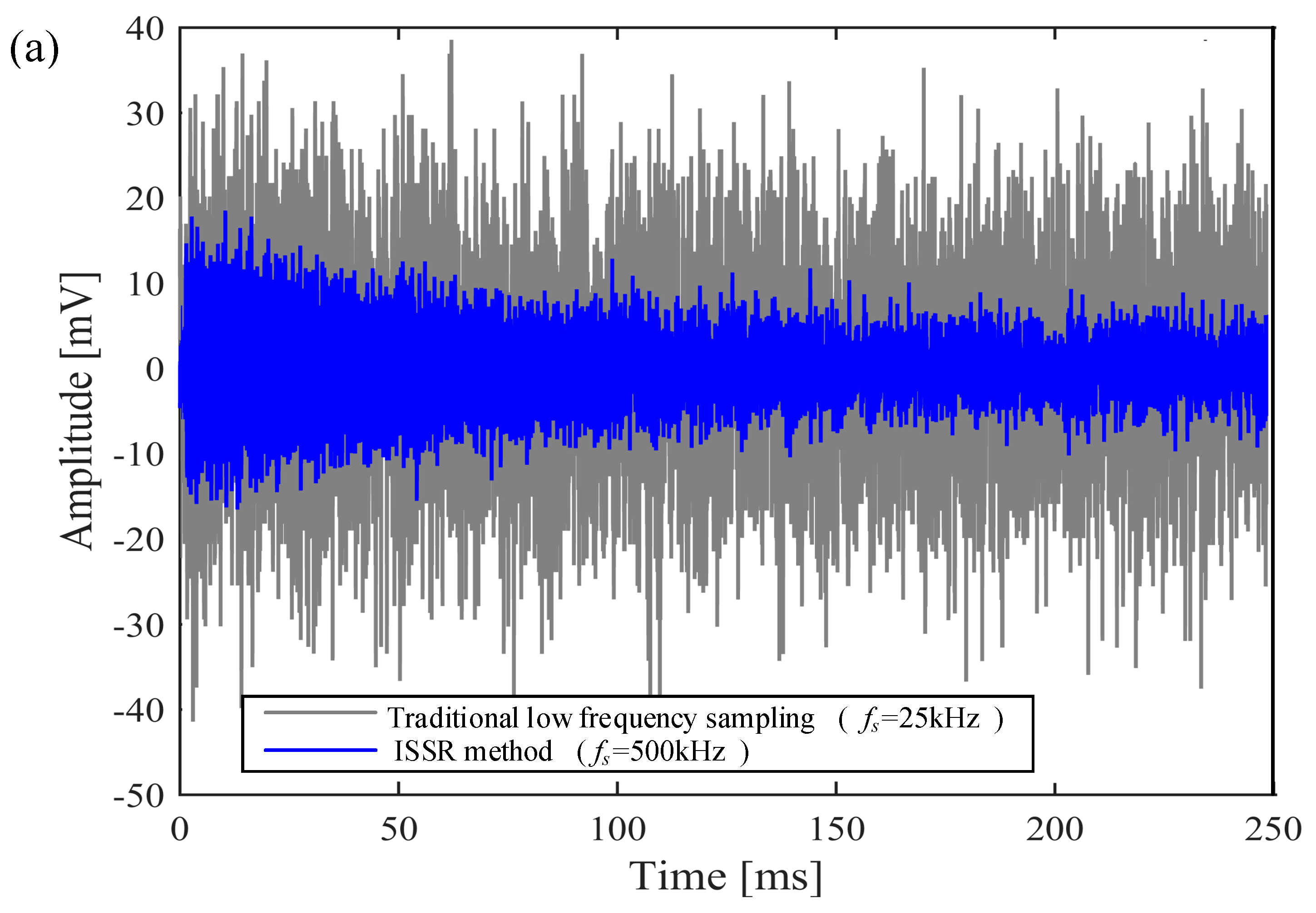
4.2. Comparison of Intensive Sampling Sparse Reconstruction and Classical Stacking Method

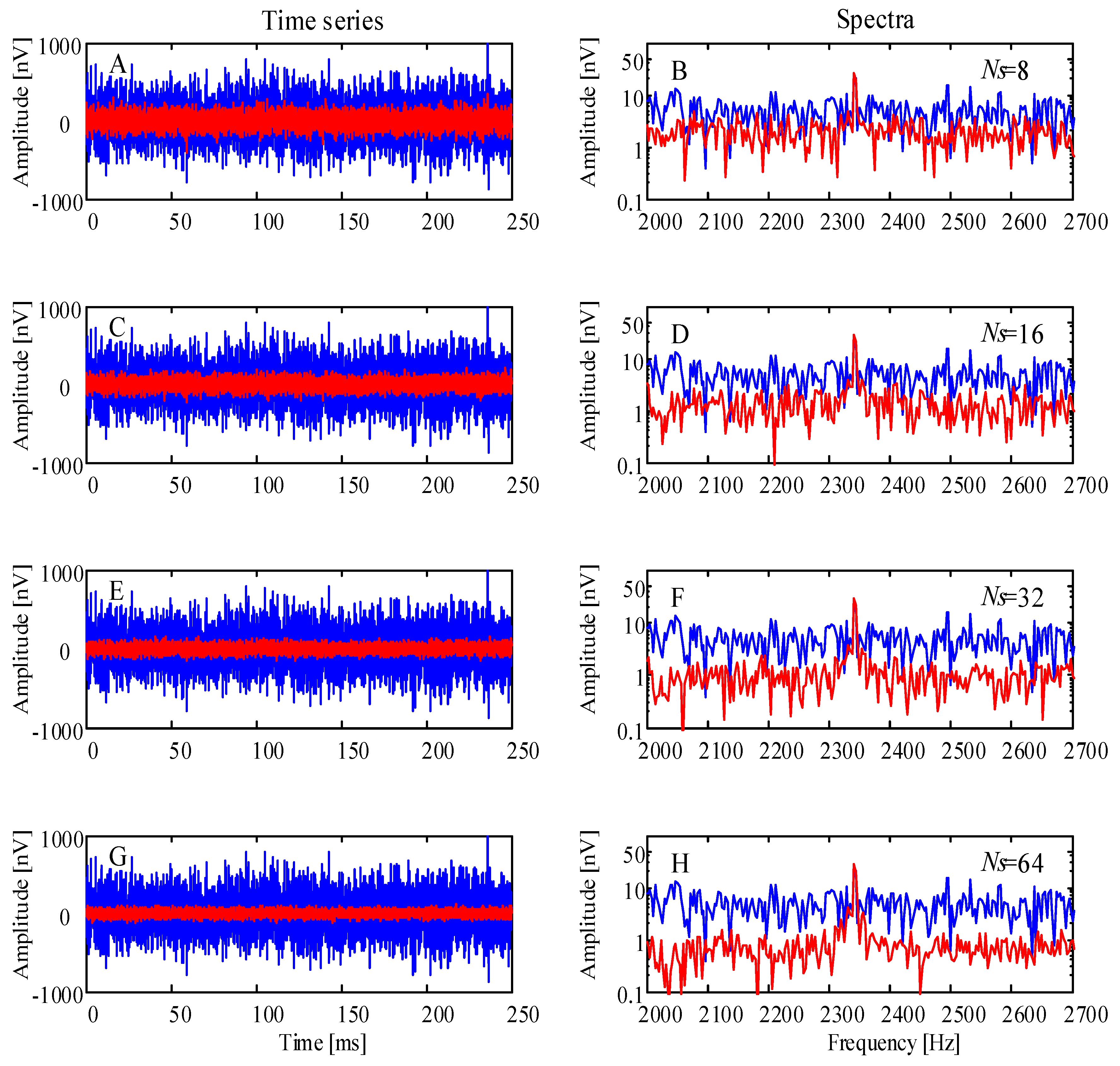
4.2.1. Simulations of Classical Stacking for Random Noise Suppression

In the simulation, the sampling frequency is 25 kHz, the acquisition time length is 250 ms, the initial amplitude of noiseless MRS signal is $U_0$ = 40.46 nV, the Larmor frequency is $f_{Larmor}$ = 2341.7 Hz, and the observed relaxation time is $T_2^{*}$ = 500 ms. The synthesized noisy signal is composed of MRS signal and Gaussian white noise. When synthesizing the noisy MRS signal, random noise is determined to be added to MRS signal based on the value of signal-to-noise ratio. In simulation, the initial SNR of synthetic noisy signal is −20 dB.

In Figure 10, the left-hand column is the time-series. The blue lines display the unstacking time-series. The red lines display the stacking time-series. The right-hand column is the spectra. The blue lines display the spectra of the unstacking time-series, and the red lines display the spectra of the stacking time-series that correspond to the left-hand column.

After suppressing random noise by 8, 16, 32 and 64 times stacking data, the SNR for power is –10.9502 dB, –7.8772 dB, –4.9493 dB, –1.9423 dB and the SNIR is 7.8387, 15.9964, 32.3185, 63.2067, respectively. The time domain waveform and the frequency domain amplitude of the stacking signals are shown in Figure 10.

In Figure 11, the first row shows the curves of power signal to noise ratio by logarithmic representation and the curves of power signal-to-noise ratio by non-logarithmic representation, respectively. The unit of SNR by logarithmic representation is dB. The unit of SNR by non-logarithmic representation is 1. The second row shows the curves of SNIR for power and MSE, respectively. The unit of SNIR for power is 1. The unit of MSE is nV². The blue lines display simulation experimental value, and the red lines display theoretical value of the power signal-to-noise ratio. SNR is a non-logarithmic representation of the power signal to noise ratio.

From Figure 11, it can be concluded that SNR and SNIR are proportional to the number of stacks and MSE is inversely proportional to the number of stacks.

4.2.2. Comparison of Intensive Sampling Sparse Reconstruction and Classical Stacking Method

Through the above simulation experiments, the rectangular sparse reconstruction has the good effect of noise suppression. Therefore, we compare the intensive sampling and sparse reconstruction of rectangular method with the classical stacking method.

From

Table 2. The classical stacking method. The estimated parameters, SNR and SNIR are reported based on the synthetic noisy MRS signal with $U_0^{}$ = 40.46 nV, $T_2^{*}$ = 500 ms, $f_{Larmor}$ = 2341.7 Hz, and initial SNR = −20 dB.

${\mathit{N}}_{\mathit{S}}$	1	8	16	32	64
$SNR(dB)$	−20	−10.9502	−7.8772	−4.9493	−1.9423
$SNIR$	1	7.8387	15.9964	32.3185	63.2067

and

Table 3. The intensive sampling rectangular sparse reconstruction. The estimated parameters, SNR and SNIR are reported based on the synthetic MRS signal with $U_0^{}$ = 40.46 nV, $T_2^{*}$ = 500 ms, $f_{Larmor}$ = 2341.7 Hz, $f_{prop}$ = 24$f_{Larmor}$ and SNR = −20 dB.

${\mathit{f}}_{{\mathit{s}}_{\mathit{H}}}(\mathbf{Hz})$	${\mathit{f}}_{\mathit{p}\mathit{r}\mathit{o}\mathit{p}}$	$\mathbf{8}{\mathit{f}}_{\mathit{p}\mathit{r}\mathit{o}\mathit{p}}$	$\mathbf{16}{\mathit{f}}_{\mathit{p}\mathit{r}\mathit{o}\mathit{p}}$	$\mathbf{32}{\mathit{f}}_{\mathit{p}\mathit{r}\mathit{o}\mathit{p}}$	$\mathbf{64}{\mathit{f}}_{\mathit{p}\mathit{r}\mathit{o}\mathit{p}}$
$SNR(\mathrm{dB})$	−20	−10.9537	−7.8869	−4.9097	−1.9680
$SNIR$	1	7.7996	15.8032	31.3668	61.7511

, it can be seen that the SNR obtained after 64 times stacks is approximately equal to that of sparse reconstruction utilizing sampling frequency $f_{s_H}=64f_{prop}$.

According to Figure 5, Figure 6, Figure 10 and Figure 11, Table 2 and Table 3, the efficiency of ISSR method is higher than that of classical stacking method based on comparing the classical stacking method with the ISSR method. Furthermore, the sparse reconstruction method has a good denoising effect. Therefore, we can increase the sampling frequency instead of multiple long-term acquisitions. Furthermore, the ISSR method can be used to improve efficiency and reduce the power consumption of the MRS instrument.

4.3. Simulation of Kernel Regression Estimation

To obtain a better denoising effect and verify the validity of kernel regression estimation, the sparse reconstructed data is subjected to kernel regression estimation processing. It should be noted that the choice of kernel has little influence on the estimation accuracy. The Gaussian kernel function is a commonly used kernel function, so this part selects the Gaussian kernel function. After the kernel function is selected, the estimation effect is affected by three factors: The regression order, the window size of kernel function, and the smoothing factor.

4.3.1. Window Size and Smoothing Factor Effect on the Estimation Result

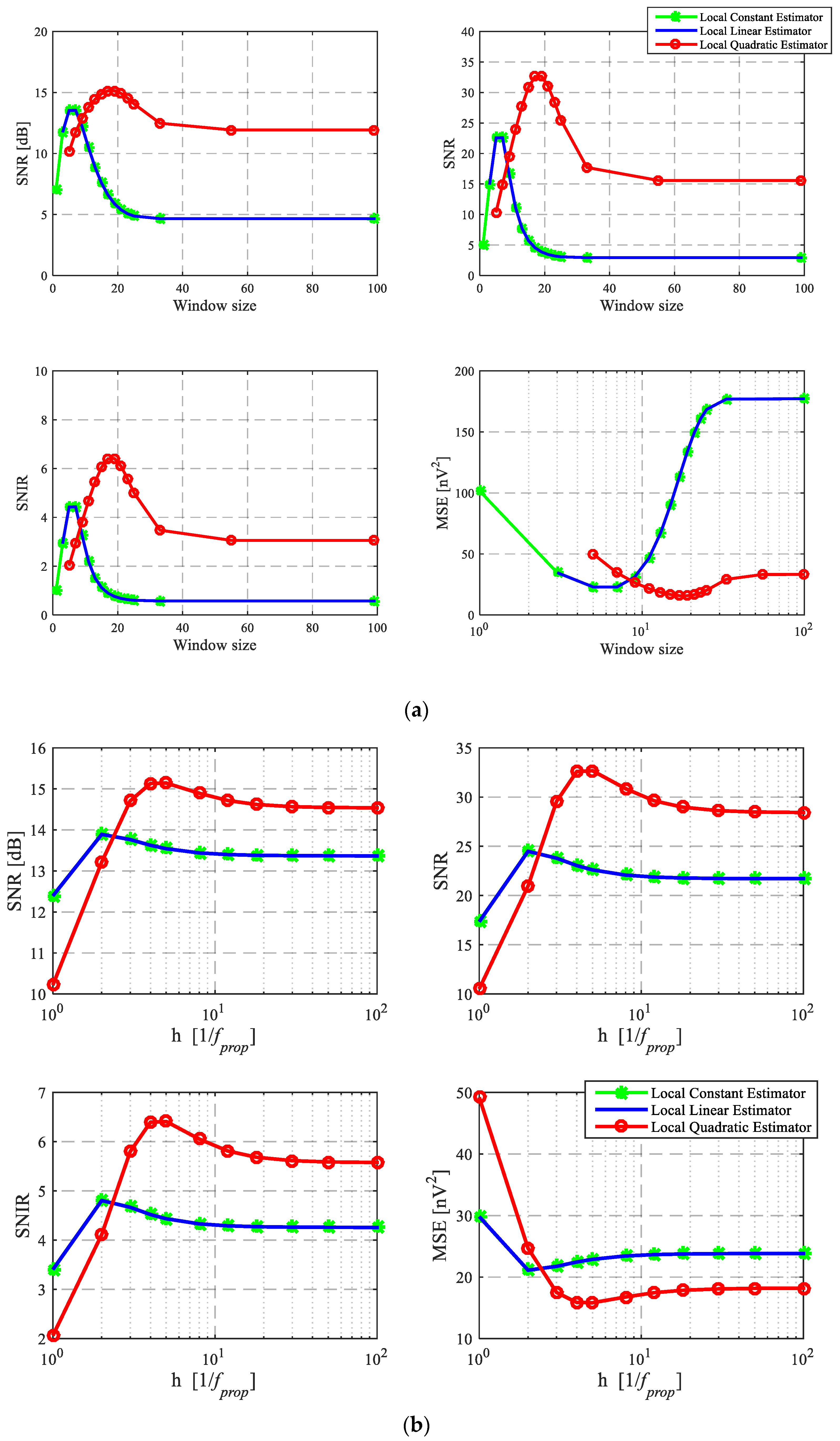
Window Size Effect

In analyzing the effect of window length on the estimation results of three different order regressions, we set the smoothing factor as a constant. The value of smoothing factor h is reasonably chosen based on a time interval of the reconstructed signal series. If the smoothing factor h is larger, the regression curve of the signal becomes smoother; otherwise the regression curve is not smooth. Here we choose the smoothing factor h to be equal to $5/f_{prop}$ where $1/f_{prop}$ is a time interval of the reconstructed signal utilizing ISSR method. In the analysis, the data to be processed by kernel regression is the data reconstructed by rectangular sparse reconstruction. The SNR of the data to be processed by kernel regression is 7.0737 dB, and $MSE$ = 101.5047 ${\mathrm{nV}}^2$.

As shown in Figure 12a, the Nadaraya–Watson estimator and the linear kernel regression estimator have a good estimation effect when the window size is 7. By these two kernel regression estimators processing, the SNR of data is 13.5430 dB. Moreover, the quadratic kernel regression estimator has a good estimation effect when the window size equals 19. By quadratic kernel regression estimator processing, the SNR of data is 15.1425 dB.

Further analysis shows that quadratic kernel regression estimator is better than linear kernel regression estimator and Nadaraya–Watson estimator when the processed data has a relatively high SNR.

Smoothing Factor Effect

With constant window size to analyze the effect of the smoothing factor $\mathrm{h}$ on the estimation results, the window size of the Nadaraya–Watson estimator, linear kernel regression estimator and quadratic kernel regression estimator is 7, 7 and 19 respectively. In the analysis, the data to be processed by kernel regression is the data reconstructed by rectangular sparse reconstruction. The SNR of the data to be processed utilizing kernel regression is SNR = 7.0737 dB, and MSE = 101.5047 nV².

From Figure 12b, when smoothing factor $h$ equals $2/f_{prop}$, Nadaraya–Watson estimator (N = 0) and linear kernel estimator (N = 1) have a good estimation effect. By these two kernel regression estimators processing, the SNR is 13.8916 dB, 13.8907 dB, respectively. For the local quadratic estimator (N = 2), it has good estimation effect when $h$ equals $5/f_{prop}$. The SNR of data is 15.1425 dB by quadratic kernel regression estimator.

4.3.2. Waveform Comparison of Kernel Regression Estimation

The data to be processed by kernel regression is the data reconstructed by rectangular sparse reconstruction, and its $SNR$ = 7.0737 dB, $MSE$ = 101.5047 ${\mathrm{nV}}^2$. In the case of a high SNR, the local quadratic estimator can obtain a higher SNR, therefore selecting a local quadratic estimator, we set its window size to 19 and its smoothing factor $h=5/f_{prop}$ for simulation experiment comparison. The waveforms and frequency domain amplitudes of kernel regression estimation are shown in Figure 13.

From Figure 12 and Figure 13, we can get that: Performing a local quadratic estimator of kernel function regression can further improve the signal SNR, such as adopting $f_s=512f_{prop}$ and by intensive sampling sparse reconstruction and local quadratic estimator. SNR increases from the initial −20 dB to 15.1425 dB, and the SNIR reaches 3267.8. From the low frequency band (1–500 Hz) and the higher frequency band (4500–5000 Hz) in the spectrogram, and the spectrum amplitude near the Larmor frequency, we can find that the local estimator of kernel function regression has a low-pass filtering effect. Increasing SNR by kernel regression estimation also causes a small attenuation of the signal amplitude. However, this attenuation effect of kernel regression estimation can be reduced by selecting appropriate estimation parameters (namely, the regression order, the window size of kernel function, and the smoothing factor).

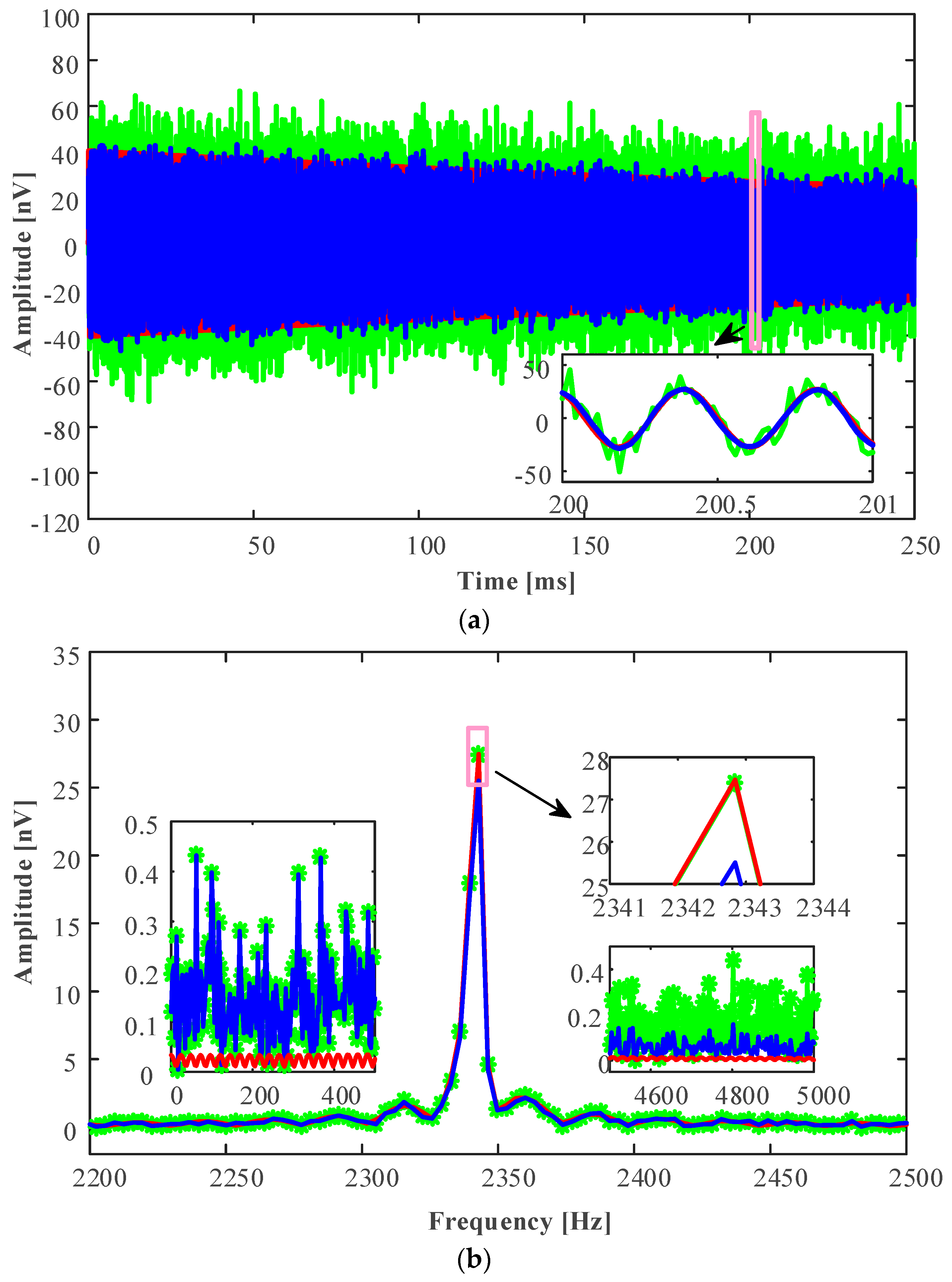
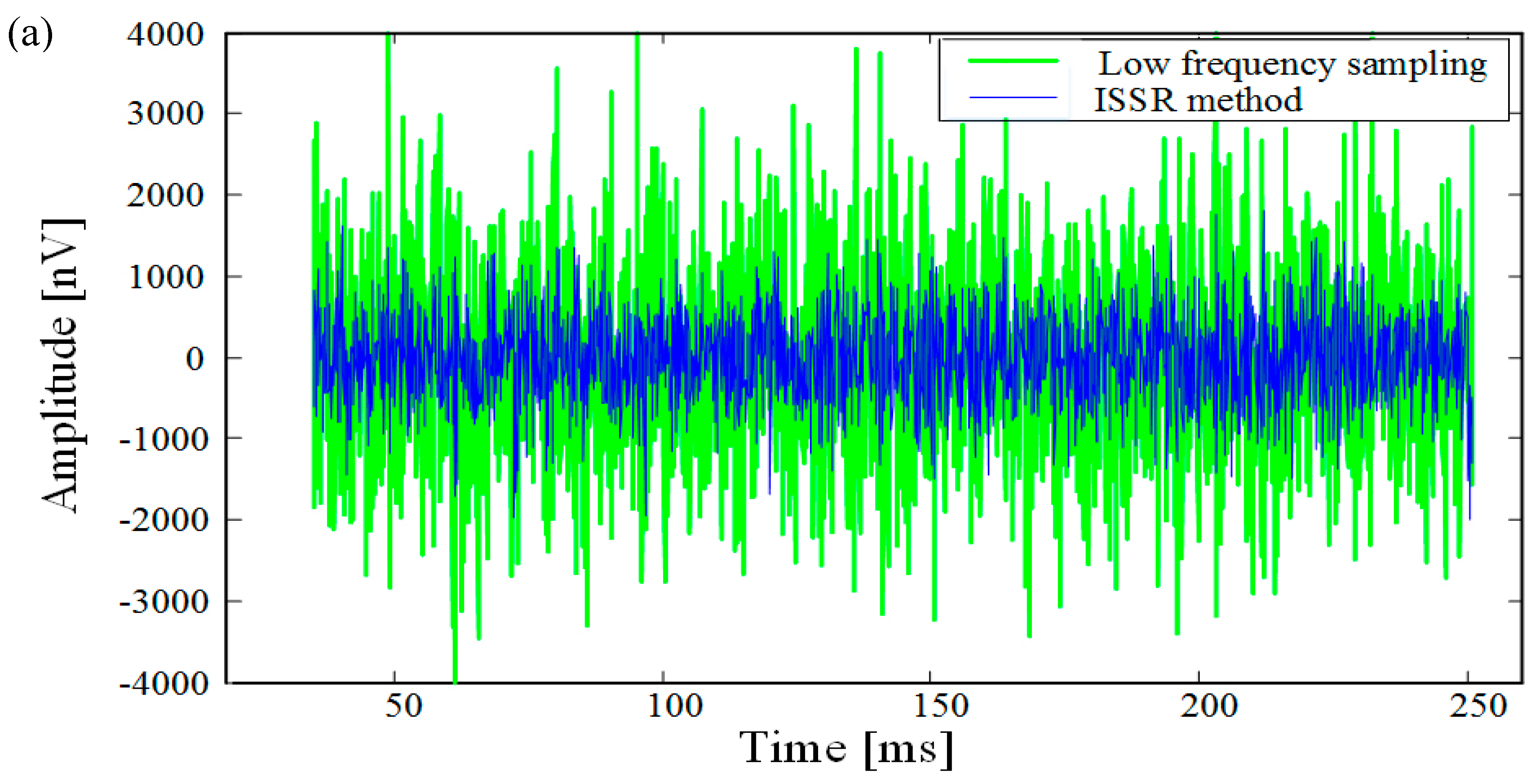
5. Field Experiments

In order to further verify the feasibility and effectiveness of the intensive sampling sparse reconstruction and kernel regression estimation, we conducted two experiments. The first experiment was carried out in laboratory and the experimental device consisted of signal generator and signal acquisition device. The second experiment was conducted in the field and the experimental setup was MRS instrument with high sampling rate.

5.1. Laboratory Experiment

In the experiment, the arbitrary waveform generator (AWG) and the signal collector were connected by a BNC (Bayonet Neill-Concelman) cable, and the signal collector acquired the noisy signal generated by the AWG signal generator. The signal collector recorded the noisy MRS signal for 250 ms at sampling frequency $f_s$ = 500 kHz, and the number of sampling points is 125,000 points. The initial amplitude of MRS signal is 5 mV and the Larmor frequency $f_{Larmor}$ is 2341.7 Hz. Calculating the solution $f_{prop}=13.3450f_{Larmor}$ according to Equation (5) and $f_{Larmor}$, then the obtained noisy data containing random noise is processed by rectangular sparse reconstruction, as shown in Figure 14.

From Figure 14, it is concluded that the reasonable $f_{prop}$ is calculated and selected, and the intensive sampling sparse reconstruction of the rectangular method can suppress noise and improve SNR. After the rectangular sparse reconstruction, SNR can be further improved by kernel regression estimation as described in Section 4.3, which is not described here.

5.2. Processing Experiment of Noisy MRS Data

The experimental data collection was carried out utilizing the MSR instrument in Shaoguo Town, Changchun City, China, as shown in Figure 15. The local Larmor frequency $f_{Larmor}$ is 2335 Hz. The single-turn transmitting coil and the single-turn receiving coil are 100 m × 100 m squares. The sampling frequency of MRS receiver is 50 kHz and a single signal acquisition time is 256 ms. The maximum transmitting peak current is 208.7556 A and the emission duration is 40 ms. The single noisy signal collected is firstly eliminated by spike noise and removed power frequency harmonics of dozens of frequencies by an adaptive notch filter.

After removing spike noise and power-frequency noise of 50 Hz multiples from the collected noisy data, there is still residual noise in data. The residual noise is not completely random noise, as shown in Figure 16. After removing the power frequency harmonics, the signal data is processed by rectangular sparse reconstruction to verify the noise elimination effect of the ISSR method, as shown in Figure 16.

In Figure 16, since the sampling frequency is only 50 kHz, the smaller $f_{prop}$ = 3.569$f_{Larmor}$ = 8333.3 Hz is calculated and selected to perform rectangular sparse reconstruction according to Equation (5).

From comparison of low frequency sampling result and the ISSR method results in Figure 16, it can be concluded that: Although the denoising ability of rectangular sparse reconstruction is weakened in the case that the noise is non-Gaussian noise, rectangular sparse reconstruction still has a certain effect of suppressing noise. In other words, the ISSR method can suppress Gaussian random noise and other types of random noise.

Furtherly, the subsequent processing is performed to verify the effect of the ISSR method and extract the MRS signal parameters. Due to low SNR of the data processed by rectangular sparse reconstruction in the experiment, local kernel regression estimation is not utilized in this case that SNR is low. In non-Gaussian random noise where the denoising effect is not excellent, we adopt a bandpass filter (bandpass range [2325 Hz 2345 Hz]) to further process the data. Finally, we process the MRS signal segment from 30 ms to 150 ms by the least squares linear fitting method to extract the initial amplitude $U_0$ = 425.42 nV and the observed relaxation time $T_2^{*}$ = 136.54 ms.

6. Discussion

We provide an approach to suppress random noise by utilizing high sampling frequency in the MRS instrument. In the approach, the basic frequency $f_{prop}$ of sparse reconstruction is one of the ISSR keys. This basic frequency is accurately calculated according to Equation (5) to avoid frequency offset and distortion of MRS signal. In the case where the sampling frequency is constant, the magnitude of basic frequency $f_{prop}$ is inversely related to the SNIR of signal in intensive sampling sparse reconstruction, as shown in Figure 9.

Three sparse reconstruction methods provide theoretical basis and specific methods for high frequency sampling to suppress random noise. These methods are feasible and have good effects according to Figure 5, Figure 6, Figure 14 and Figure 16. The rectangular sparse reconstruction and trapezoidal sparse reconstruction are better than Simpson sparse reconstruction in terms of the suppression effect of random noise (especially, in suppressing Gaussian random noise), from Figure 7a–c and Table 1 in Section 4 and Equations (7)–(12) in Section 3.2.3 for details. This order is the opposite of the order of the three numerical integration effects. This phenomenon of order inconsistency is caused by noise interference. By comparing the classical stacking method and the intensive sampling sparse reconstruction in the paper, we can increase sampling frequency instead of multiple long-term recordings of classical stacking method, and improve the efficiency of the instrument, seeing Figure 5, Figure 6, Figure 10 and Figure 11, Table 2 and Table 3. Besides, these sparse reconstruction methods lay a theoretical foundation for the compression of MRS data with high sampling frequency. The sparse reconstruction method has a good effect in suppressing random noise, but it also has limitations such as poor performance in suppressing harmonic noise and requiring high sampling frequency. In terms of sparse reconstruction limitation in Section 5.2, for example, when there is a large amount of non-Gaussian noise such as harmonic noise, the effect of sparse reconstruction method is weakened and it needs combination with other filtering methods.

The kernel regression estimation introduced in this paper provides a feasible method for suppressing noise in MRS data with high SNR, seeing Figure 13. To obtain better regression estimation results, we should pay attention to the selection of reasonable window size, order, and the smoothing factor according to Figure 12. In addition, the regression estimation does not work well in the case of large noise.

The intensive sampling sparse reconstruction approach has fewer recording times, less transmitting energy consumption and higher efficiency in terms of instrument transmission and reception. Furthermore, the approach provides theoretical guidance and specific methods for high or variable frequency sampling to suppress random noise. At the same time, the approach gives a research direction for the development of MRS instruments with low power consumption and high work efficiency. In addition, the intensive sampling sparse reconstruction approach can also be applied to suppressing random noise in other geophysical signal processing or other signal processing areas. In the future, we will endeavour to overcome the limitations of ISSR-KRE and to handle other types of noise (i.e., harmonic noise, spike noise) in combination with other methods.

7. Conclusions

In order to better suppress random noise in MRS data, we propose an approach of intensive sampling sparse reconstruction and kernel regression estimation to improve SNR in this paper. The approach is based on variable frequency sampling, numerical integration and statistical signal processing combined with kernel regression estimation. Furthermore, we propose three specific sparse reconstructions (i.e., rectangular sparse reconstruction, trapezoidal sparse reconstruction and Simpson sparse reconstruction) to realize intensive sampling sparse reconstruction. By means of simulative experiments, we find that all three sparse reconstructions can suppress random noise, and rectangular sparse reconstruction and trapezoidal sparse reconstruction are better than Simpson sparse reconstruction in terms of the suppression effect of random noise. At the same time, we verify the positive correlation of SNIR and sampling frequency. Besides, compared with the classical stacking method, the sparse reconstruction method has high efficiency and good denoising effect. In a simulation example, the ISSR is utilized to process noisy MRS data, and SNR is improved by 27.0737 dB. Further, in simulation of kernel regression estimation, we find that the suppression effect of kernel regression is related to Taylor order, window size and smoothing factor. Hence, we should choose kernel regression estimation with appropriate parameters to reduce random noise. In coping with the data processed by the ISSR, SNR is increased by 8.0688 dB adopting the KRE. In other words, the ISSR-KRE approach improved SNR by 35.1425 dB. Furthermore, in both the laboratory experiment and the field experiment of the MRS instrument, we verify the feasibility and effectiveness of the ISSR-KRE approach to suppress random noise by processing the data sampled at different sampling frequencies, such as 500 kHz and 50 kHz. For example, in processing noisy MRS data, the standard deviation of the data is reduced from 1200.80 nV to 570.01 nV utilizing the ISSR. The proposed approach and specific methods provide theoretical support for random noise suppression. In addition, the approach contributes to sampling method and the development of MRS instrument with low power consumption and high efficiency. In the future, we will integrate the approach and the methods into the hardware system of MRS instrument and attempt to utilize these methods to eliminate power frequency noise.

References

1. Hertrich, M.; Braun, M.; Gunther, T.; Green, A.G.; Yaramanci, U. Surface nuclear magnetic resonance tomography. IEEE Trans. Geosci. Remote Sens. 2007, 45, 3752–3759. [Google Scholar] [CrossRef]
2. Legchenko, A.; Valla, P. Removal of power-line harmonics from proton magnetic resonance measurements. J. Appl. Geophys. 2003, 53, 10–120. [Google Scholar] [CrossRef]
3. Liu, L.; Grombacher, D.; Auken, E.; Larsen, J.J. Removal of Co-Frequency Powerline Harmonics from Multichannel Surface NMR Data. IEEE Geosci. Remote Sens. Lett. 2018, 15, 53–57. [Google Scholar] [CrossRef]
4. Chen, H.M.; Wang, H.C.; Chai, J.W.; Chen, C.C.C.; Xue, B.; Wang, L.; Yu, C.; Wang, Y.; Song, M.; Chang, C.I. A Hyperspectral Imaging Approach to White Matter Hyperintensities Detection in Brain Magnetic Resonance Images. Remote Sens. 2017, 9, 1174. [Google Scholar] [CrossRef]
5. Powers, J.M.; Ioachim, G.; Stroman, P.W. Ten Key Insights into the Use of Spinal Cord fMRI. Brain Sci. 2018, 8, 173. [Google Scholar] [CrossRef] [PubMed]
6. Legchenko, A.; Descloitres, M.; Bost, A.; Ruiz, L.; Reddy, M.; Girard, J.F.; Sekhar, M.; Kumar, M.S.M.; Braun, J.J. Resolution of MRS applied to the characterization of hard-rock aquifers. Groundwater 2006, 44, 547–554. [Google Scholar] [CrossRef] [PubMed]
7. Walsh, D.O. Multi-channel surface NMR instrumentation and software for 1D/2D groundwater investigations. J. Appl. Geophys. 2008, 66, 140–150. [Google Scholar] [CrossRef]
8. Qin, S.; Ma, Z.; Jiang, C.; Lin, J.; Xue, Y.; Shang, X.; Li, Z. Response Characteristics and Experimental Study of Underground Magnetic Resonance Sounding Using a Small-Coil Sensor. Sensors 2017, 17, 2127. [Google Scholar] [CrossRef]
9. Valois, R.; Vouillamoz, J.M.; Lun, S.; Arnout, L. Mapping groundwater reserves in northwestern Cambodia with the combined use of data from lithologs and time-domain-electromagnetic and magnetic-resonance soundings. Hydrogeol. J. 2018, 26, 1187–1200. [Google Scholar] [CrossRef]
10. Parsekian, A.D.; Creighton, A.L.; Jones, B.M.; Arp, C.D. Surface nuclear magnetic resonance observations of permafrost thaw below floating, bedfast and transitional ice lakes. Geophysics 2019, 84, EN33–EN45. [Google Scholar] [CrossRef]
11. Garambois, S.; Legchenko, A.; Vincent, C.; Thibert, E. Ground-penetrating radar and surface nuclear magnetic resonance monitoring of an englacial water-filled cavity in the polythermal glacier of Tete Rousse. Geophysics 2016, 81, WA131–WA146. [Google Scholar] [CrossRef]
12. Shang, X.; Jiang, C.; Ma, Z.; Qin, S. Combined System of Magnetic Resonance Sounding and Time-Domain Electromagnetic Method for Water-Induced Disaster Detection in Tunnels. Sensors 2018, 18, 3508. [Google Scholar] [CrossRef] [PubMed]
13. Falzone, S.; Keating, K. Algorithms for removing surface water signals from surface nuclear magnetic resonance infiltration surveys. Geophysics 2016, 81, WB97–WB107. [Google Scholar] [CrossRef]
14. Ghanati, R.; Hafizi, M.K.; Fallahsafari, M. Surface nuclear magnetic resonance signals recovery by integration of a non-linear decomposition method with statistical analysis. Geophys. Prospect. 2016, 64, 489–504. [Google Scholar] [CrossRef]
15. Liu, L.; Grombacher, D.; Auken, E.; Larsen, J.J. Complex envelope retrieval for surface nuclear magnetic resonance data using spectral analysis. Geophys. J. Int. 2019, 217, 894–905. [Google Scholar] [CrossRef]
16. Jiang, C.; Lin, J.; Duan, Q.; Sun, S.; Tian, B. Statistical stacking and adaptive notch filter to remove high-level electromagnetic noise from MRS measurements. Near Surf. Geophys. 2011, 9, 459–468. [Google Scholar] [CrossRef]
17. Larsen, J.J. Model-based subtraction of spikes from surface nuclear magnetic resonance data. Geophysics 2016, 81, WB1–WB8. [Google Scholar] [CrossRef] [Green Version]
18. Larsen, J.; Dalgaard, E.; Auken, E. Noise cancelling of MRS signals combining model-based removal of powerline harmonics and multichannel Wiener filtering. Geophys. J. Int. 2014, 196, 828–836. [Google Scholar] [CrossRef]
19. Wang, Q.; Jiang, C.; Mueller-Petke, M. An alternative approach to handling co-frequency harmonics in surface nuclear magnetic resonance data. Geophys. J. Int. 2018, 215, 1962–1973. [Google Scholar] [CrossRef]
20. Dalgaard, E.; Christiansen, P.; Larsen, J.J.; Auken, E. A temporal and spatial analysis of anthropogenic noise sources affecting SNMR. J. Appl. Geophys. 2014, 110, 34–42. [Google Scholar] [CrossRef]
21. Legchenko, A.; Valla, P. Processing of surface proton magnetic resonance signals using non-linear fitting. J. Appl. Geophys. 1998, 39, 77–83. [Google Scholar] [CrossRef]
22. Dalgaard, E.; Auken, E.; Larsen, J.J. Adaptive noise cancelling of multichannel magnetic resonance sounding signals. Geophys. J. Int. 2012, 191, 88–100. [Google Scholar] [CrossRef]
23. Ghanati, R.; Hafizi, M.K.; Mahmoudvand, R.; Fallahsafari, M. Filtering and parameter estimation of surface-NMR data using singular spectrum analysis. J. Appl. Geophys. 2016, 130, 118–130. [Google Scholar] [CrossRef]
24. Lin, T.; Zhang, Y.; Yi, X.; Fan, T.; Wan, L. Time-frequency peak filtering for random noise attenuation of magnetic resonance sounding signal. Geophys. J. Int. 2018, 213, 727–738. [Google Scholar] [CrossRef]
25. Trushkin, D.V.; Shushakov, O.A.; Legchenko, A. The potential of a noise-reducing antenna for surface NMR groundwater surveys in the Earth’s magnetic field. Geophys. Prospect. 1994, 42, 855–862. [Google Scholar] [CrossRef]
26. Behroozmand, A.A.; Auken, E.; Fiandaca, G.; Rejkjaer, S. Increasing the resolution and the signal-to-noise ratio of magnetic resonance sounding data using a central loop configuration. Geophys. J. Int. 2016, 205, 243–256. [Google Scholar] [CrossRef] [Green Version]
27. Karine, A.; Toumi, A.; Khenchaf, A.; El Hassouni, M. Radar Target Recognition Using Salient Keypoint Descriptors and Multitask Sparse Representation. Remote Sens. 2018, 10, 843. [Google Scholar] [CrossRef]
28. Zhang, J.; Zeng, Z.; Zhang, L.; Lu, Q.; Wang, K. Application of Mathematical Morphological Filtering to Improve the Resolution of Chang’E-3 Lunar Penetrating Radar Data. Remote Sens. 2019, 11, 524. [Google Scholar] [CrossRef]
29. Takeda, H.; Farsiu, S.; Milanfar, P. Kernel Regression for Image Processing and Reconstruction. IEEE Trans. Image Process. 2007, 16, 349–366. [Google Scholar] [CrossRef] [Green Version]
30. Legchenko, A. Magnetic Resonance Imaging for Groundwater; ISTE Ltd: London, UK, 2013. [Google Scholar]
31. Legchenko, A.; Valla, P. A review of the basic principles for proton magnetic resonance sounding measurements. J. Appl. Geophys. 2002, 50, 3–19. [Google Scholar] [CrossRef]
32. Li, Q.; Wang, N.; Yi, D. Numerical Analysis, 5th ed.; Tsinghua University Press: Beijing, China, 2008; pp. 97–135. [Google Scholar]
33. Sheng, Z.; Xie, S.; Pan, C. Probability Theory and Mathematical Statistics, 4th ed.; Higher Education Press: Beijing, China, 2008; pp. 76–83. [Google Scholar]
Figure 1. Schematic diagram for detection of magnetic resonance sounding (MRS) signal.
Remotesensing 11 01829 g001
Figure 2. Flowchart for implementation of the intensive sampling sparse reconstruction and kernel regression estimation (ISSR-KRE) approach.
Remotesensing 11 01829 g002
Figure 3. Schematic diagram of intensive sampling sparse reconstruction.
Remotesensing 11 01829 g003
Figure 4. A data fragment of intensive sampling in [ t a j , t b j ] .
Remotesensing 11 01829 g004
Figure 5. Simulation case: Comparison of suppressing random noise effect of rectangular sparse reconstruction by different sampling frequencies f s H . Time-series and spectra of the sampling frequencies 8 f p r o p , 16 f p r o p , 32 f p r o p , and 64 f p r o p , respectively.
Remotesensing 11 01829 g005
Figure 6. The curves of signal to noise ratio (SNR), signal-to-noise improvement ratio (SNIR), mean squared error (MSE) with increasing sampling frequency by rectangular sparse reconstruction.
Remotesensing 11 01829 g006
Figure 7. Comparison of three sparse reconstruction methods (rectangular sparse reconstruction, trapezoidal sparse reconstruction and Simpson sparse reconstruction): (a) SNR comparison, (b) SNIR comparison, (c) MSE comparison.
Remotesensing 11 01829 g007aRemotesensing 11 01829 g007b
Figure 8. Comparison of rectangular sparse reconstruction, trapezoidal sparse reconstruction and Simpson sparse reconstruction for processing signals. (a) Time domain, (b) frequency domain.
Remotesensing 11 01829 g008
Figure 9. Different f p r o p effect on sparse reconstruction. The first row shows the comparison of SNR in different f p r o p cases, respectively. The second row shows the comparison of SNIR and MSE in different f p r o p cases, respectively.
Remotesensing 11 01829 g009
Figure 10. Simulation case: Time-series and spectra of 8, 16, 32, 64 stacks at one pulse moment, respectively.
Remotesensing 11 01829 g010
Figure 11. The curves of SNR, SNIR and MSE with increasing stacking times.
Remotesensing 11 01829 g011
Figure 12. The effect of kernel regression parameters on estimation results. (a) The effect of window size. (b) The effect of the smoothing factor h.
Remotesensing 11 01829 g012
Figure 13. Waveform comparison of the data processed by the local quadratic estimator (window size 19 and smoothing factor h = 5 / f p r o p ). (a) Comparison in time domain. (b) Comparison in frequency domain. The green lines display the data by the rectangular sparse reconstruction method. The red lines display the ideal signal. The blue lines display the data by the rectangular sparse reconstruction method and the local quadratic kernel regression estimation. In other words, the blue lines display the ISSR-KRE data.
Remotesensing 11 01829 g013
Figure 14. Comparison of traditional low frequency sampling and the ISSR method. The gray lines display traditional low frequency sampling recording. The blue lines display the data processed by the ISSR method. (a) Comparison in time domain. (b) Comparison in frequency domain.
Remotesensing 11 01829 g014aRemotesensing 11 01829 g014b
Figure 15. Field experiment location and the MRS instrument.
Remotesensing 11 01829 g015
Figure 16. Comparison of low frequency sampling result and the ISSR method results. The green lines display low frequency sampling recording (its sampling frequency is 8330 Hz) and the standard deviation is 1200.80 nV. The blue lines display the data by the ISSR method (its sampling frequency is 50 kHz, f p r o p = 8333.3 Hz) and the standard deviation is 570.01 nV. (a) Comparison in time domain. (b) Comparison in frequency domain.
Remotesensing 11 01829 g016aRemotesensing 11 01829 g016b