Article

A Metric for Evaluating the Geometric Quality of Land Cover Maps Generated with Contextual Features from High-Dimensional Satellite Image Time Series without Dense Reference Data

1
CESBIO, CNES, CNRS, IRD, UPS, Université de Toulouse, 31400 Toulouse, France
2
Centre National d’Etudes Spatiales, 18 avenue Edouard Belin, 31400 Toulouse, France
*
Author to whom correspondence should be addressed.
Remote Sens. 2019, 11(16), 1929; https://0-doi-org.brum.beds.ac.uk/10.3390/rs11161929
Submission received: 14 June 2019 / Revised: 16 July 2019 / Accepted: 18 July 2019 / Published: 17 August 2019
(This article belongs to the Section Remote Sensing Image Processing)

Abstract

:
Land cover maps are a key resource for many studies in Earth Observation, and thanks to the high temporal, spatial, and spectral resolutions of systems like Sentinel-2, maps with a wide variety of land cover classes can now be automatically produced over vast areas. However, certain context-dependent classes, such as urban areas, remain challenging to classify correctly with pixel-based methods. Including contextual information into the classification can either be done at the feature level with texture descriptors or object-based approaches, or in the classification model itself, as is done in Convolutional Neural Networks. This improves recognition rates of these classes, but sometimes deteriorates the fine-resolution geometry of the output map, particularly in sharp corners and in fine elements such as rivers and roads. However, the quality of the geometry is difficult to assess in the absence of dense training data, which is usually the case in land cover mapping, especially over wide areas. This work presents a framework for measuring the geometric precision of a classification map, in order to provide deeper insight into the consequences of the use of various contextual features, when dense validation data is not available. This quantitative metric, named the Pixel Based Corner Match (PBCM), is based on corner detection and corner matching between a pixel-based classification result, and a contextual classification result. The selected case study is the classification of Sentinel-2 multi-spectral image time series, with a rich nomenclature containing context-dependent classes. To demonstrate the added value of the proposed metric, three spatial support shapes (window, object, superpixel) are compared according to their ability to improve the classification performance on this challenging problem, while paying attention to the geometric precision of the result. The results show that superpixels are the best candidate for the local statistics features, as they modestly improve the classification accuracy, while preserving the geometric elements in the image. Furthermore, the density of edges in a sliding window provides a significant boost in accuracy, and maintains a high geometric precision.

1. Introduction

Satellite image time series capture the temporal evolution of the optical properties of land surfaces, and their use allows certain land cover classes, such as crops, to be classified with a high accuracy. Several studies [1,2,3,4], show that the time series of each pixel is a rich source of discriminatory features for producing land cover classification maps. These are maps where each pixel bears a categorical label describing the land cover of the corresponding area. However, certain classes remain difficult to identify correctly, even with multi-temporal and multi-spectral information. For example, shrublands are often confused with forests, as the difference between the two classes is the density of tree cover. In the same way, continuous urban fabric, roads, and industrial and commercial units all present high confusion rates [5]. Indeed, the main difference between buildings situated in a dense city center and buildings in a suburban residential area lies in the quantity of vegetation surrounding each building. In other words, it is the spatial arrangement of the buildings and vegetation in the proximity, more than the characteristics of each building itself, which is discriminatory.
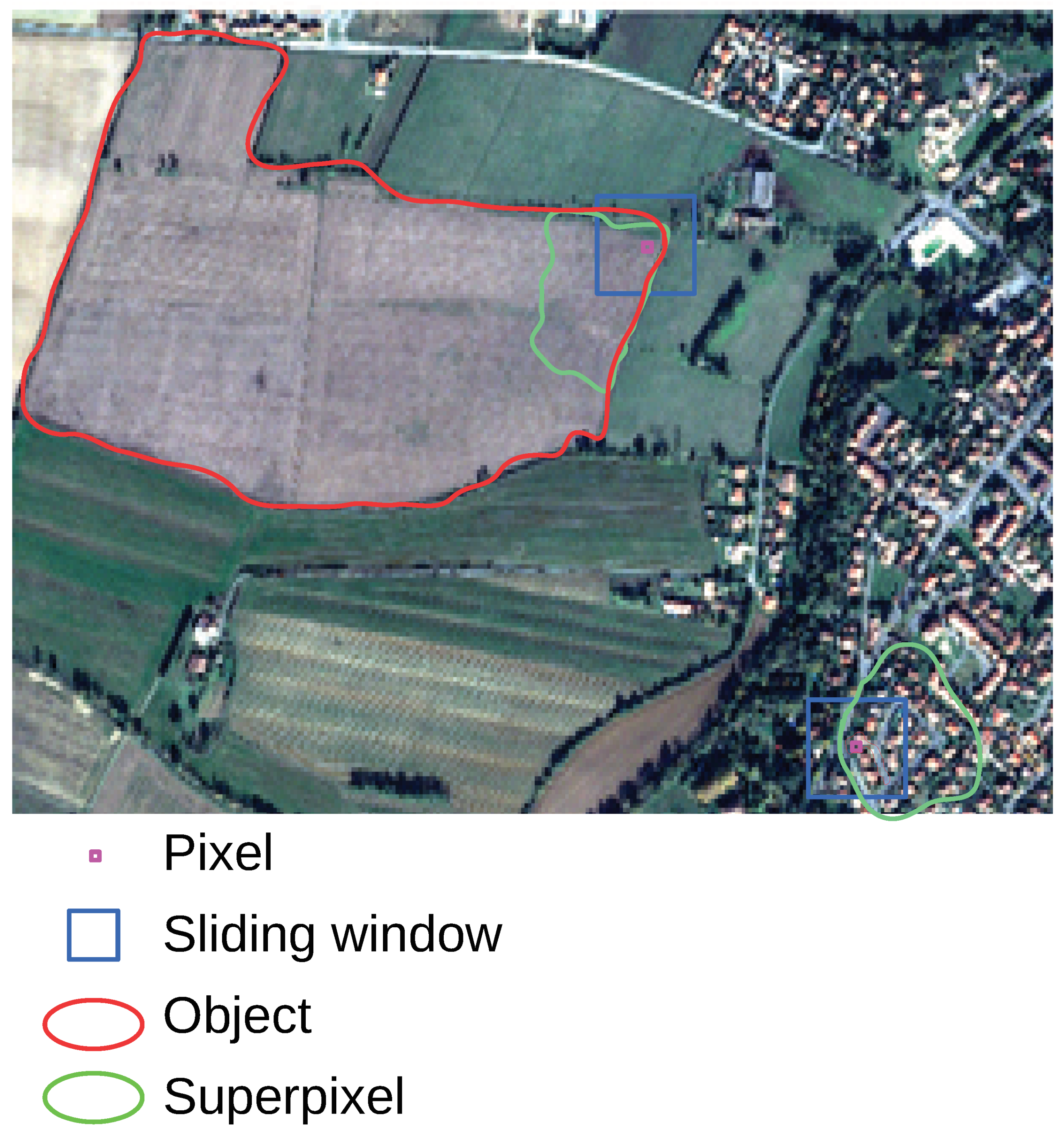
Over the past decades, there has been a steady increase in the availability of high spatial resolution satellite imagery, bringing to light new details that were previously inaccessible with lower spatial resolution images. For example, fine elements such as roads, lone trees or houses, as well as their textures can be captured at a 10 m spatial resolution with Sentinel-2 images. Using such images, it seems relevant to seek to describe groups of adjacent pixels in the image rather than individual pixels. Indeed, at such a spatial resolution, the pixels are often smaller than the objects containing them, so the spatial arrangement of these pixels can help to describe and to distinguish the various objects present in the image. In this paper, features that describe a group of adjacent pixels in an image are called contextual features, and the group of pixels in question is called the spatial support of the feature.
A very common approach is to consider a sliding window around each pixel as spatial support. The central pixel is often described with contextual information like textures, a common example being the Haralick textures [6], which are based on the Gray Level Co-Occurence Matrix, and have previously been used in Remote Sensing classification problems [7,8]. These contextual features are then included into a classification scheme by using a classifier adapted for multi-modal inputs, like a Composite Kernel SVM [9,10], or a Random Forest [11].
In other recent works, Convolutional Neural Networks have been applied to land cover mapping problems [12,13,14]. In such approaches, the contextual information is directly included in the classification model, through the convolutional layers of the network. These networks either assign one label to the central pixel of each input patch (networks such as AlexNet [15]), or provide a dense labeling of the entire patch (e.g., U-Net [16]).
While using a sliding window brings an interesting characterization of the neighboring pixels, it also can lead to a smoothing of the sharp corners and fine elements in the output map. Indeed, when using a square support, there is a risk of the relevant context being drowned out by the description of neighboring image objects, especially if the pixel is surrounded by very different objects. This may lead to confusion between the pixel class and its neighboring classes, as the pixel would adopt a very similar contextual characterization as the neighbors. Generally speaking, pixels belonging to sharp corners, or fine elements such as roads and rivers in land cover mapping are sensitive to this phenomenon. This is demonstrated in the experiments in Section 5.
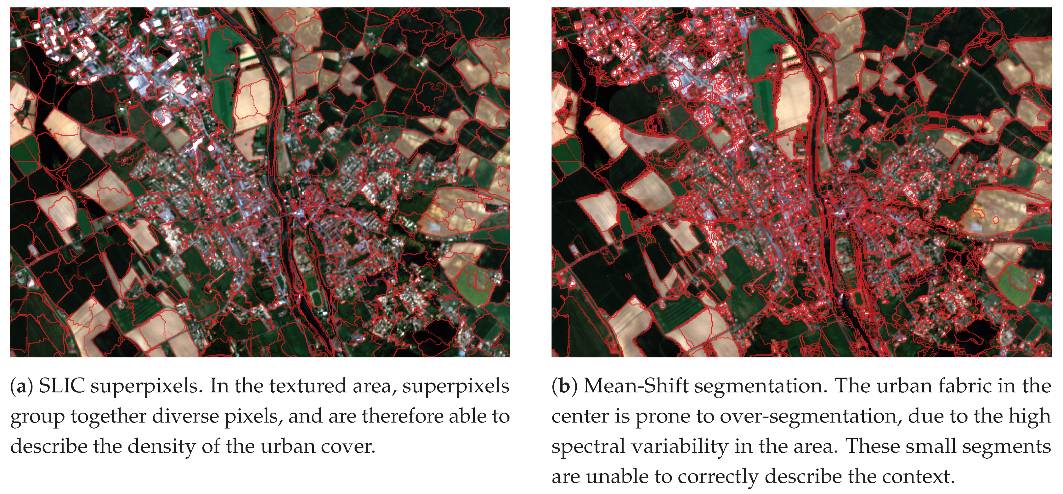
Another approach is to consider a spatial support adaptive to the nearby image content, which leads to methods based on image segmentation, such as Object Based Image Analysis (OBIA) [17], which is also commonly used in remote sensing [18,19]. However, this comes at the risk of not including a sufficient diversity of pixels to characterize the context, especially in textured areas, due to over-segmentation. For this reason, superpixels [20], which offer an intermediate representation between sliding windows and objects, have also been used in other studies [21,22]. More details about this trade-off and about superpixels can be found in Section 3.3.
In any case, evaluating the quality of a contextual classification must be done with care, as some methods have the tendency to alter the geometry of the output map. The usual statistical performance indicators (Overall Accuracy, Cohen’s κ , and F-score) are naturally biased towards the most common samples in the validation data set, meaning that high spatial frequency elements, such as corners and fine elements, are usually poorly represented in the validation. This implies that errors in such areas have a low influence on the overall statistical performance indicators. In other words, the deterioration of high spatial frequency areas can be overshadowed by other effects, such as the smoothing of noisy pixels in homogeneous areas.
One way to evaluate the quality of the geometry of a classification map is to split the validation set in several subsets, where each subset contains pixels of a certain geometric category, such as corners, edges, or central areas, as is done in [23], and later in [24]. This allows a specific measurement of the deterioration of the various geometric entities in the image, but requires dense reference data to categorize the validation labels as corners, edges, etc. Another commonly used metric, the Intersection over Union (IoU) [25] also requires dense reference data to calculate the areas of intersection and union. Moreover, it is subject to the same biases as Overall Accuracy and κ , as it measures an average error on the target object or segment. The more sophisticated Overall Geometric Accuracy (OGA) proposed by [26] also uses the areas of intersection and union, in combination with the position of the center of gravity of the reference and target objects. However, using such metrics is only possible if the validation data set is dense, in other words, if every pixel of the training area is labeled. Indeed, without this information, there is no way to split the validation data into geometric categories, or to extract the reference objects.
Unfortunately, dense validation data is not available in most practical land cover problems. Indeed, there are many cases where training data is manually collected in the field, or comes from a combination of existing data bases, which are all incomplete, or for which certain classes are out of date. A small, dense validation set could be manually constructed, but this would limit the metric to a reduced region, and would be a very time-consuming process. 
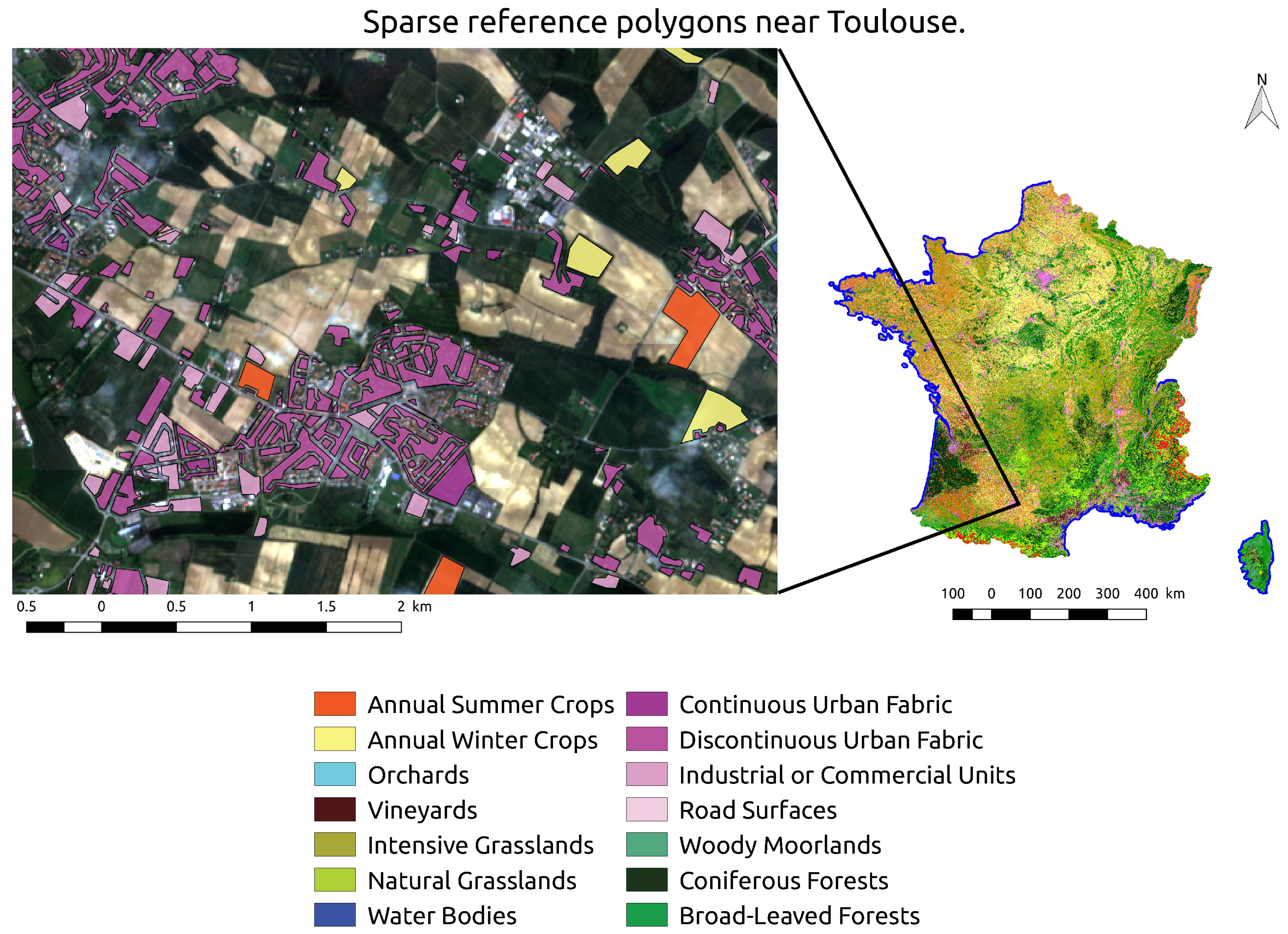
Figure 1 illustrates the sparse reference data used later in the Experimental Section, which is similar to the database used in [5] for time series mapping over France. The validation data contains polygons that unfortunately do not contain a full description of the geometry. First of all, the polygons have been eroded, to limit the negative impact of spatial co-registration errors between different images at dates. Second of all, the edges and corners of the polygons can not be used as reference geometry, because there is no guarantee that each polygon edge truly separates elements of two different classes.
The objective of this study is therefore to present a metric that can measure the geometric quality of a classification map, even when the validation data is sparsely distributed across the image, as is the case in many land cover mapping problems [5,13,14].
By comparing a contextual classification to a pixel-based classification, instead of a dense reference data set, it is possible to measure how well certain geometric elements, which are usually well recognized by pixel-based classifiers, are preserved. In other words, the pixel-based classification can be used as an approximation of the dense reference data set, at least for some class borders. Sharp corners are commonly subject to the smoothing effects visible in many contextual classification maps, and are relatively simple to identify in a such a map using currently existing corner extraction methods. For this reason, the precise localization of sharp corners is considered as an indicator of the quality of the geometry in the output map. Further details about the supervised corner extraction method, and about its validation, are given in Section 2.
This study proposes a new metric called the Pixel Based Corner Match (PBCM), which is evaluated on classification results generated with contextual features from three different spatial supports: sliding windows, objects from an object segmentation, and superpixels. A precise definition and more information regarding each method is given in Section 3. In a previous study [27], these three spatial supports were compared in terms of how much they influenced the classification accuracy, especially of classes that depend heavily on context. The performance of the methods was evaluated using only the standard classification accuracy metrics and on a unique area of 110 km × 110 km. The authors concluded that the geometric precision of the result should be analyzed quantitatively, as some of the contextual classification methods have a tendency to deform the geometry of the output.
The case study is the challenging problem of satellite image time series classification, based on Sentinel-2 imagery, which presents several practical difficulties, in particular, a very high number of features in the original feature space due to the combined use of multi-spectral and multi-temporal information, a certain degree of label noise, and a lack of densely available reference data [5,28]. Therefore, care must be taken when selecting which contextual classification method to apply, which is the underlying motivation behind this study.
The rest of the paper is organized as follows. The details of the new Pixel Based Corner Match (PBCM) geometric accuracy metric, are provided in Section 2. Then, the various strategies for defining the spatial support are detailed in Section 3. Next, Section 4 focuses on the two types of contextual features used in the experiments. The experimental setup is given in Section 5, and the results in Section 6. Finally, Section 7 draws conclusions and suggests perspectives for future studies.

2. Pixel Based Corner Match to Measure Geometric Precision

In this section, a new metric that aims to quantify the geometric precision of a contextual method, with respect to a pixel-based method is presented. This metric relies on the output of a pixel-based classifier to extract sharp corners, which are compared to the corners from a contextual classification map. This is based on the assumption that the pixel-based classification map respects the high spatial frequency areas, and the target geometry. Indeed, a pixel-based classification map can be sensitive to noise and to errors in context dependent classes, but it should preserve the corners and fine elements in the image. On the other hand, context-based classifiers can alter the geometry of the result. An example of this phenomenon is given later, in the Experimental Section in Figure 14c, in which many of the sharp corners originally present in the pixel-based classification are smoothed when using a contextual method. For these reasons, the PBCM is based on corner detection alone, with the pixel-based classification map used as a reference.
The image itself should not be used to detect the reference corners, because highly textured areas contain many corners which should not be present in the target classification maps. In other words, the corners that should be preserved by a contextual classifier are the ones at the intersections of the different classes, which are not necessarily the same as the corners in the actual image.
Using successive steps of line detection and corner detection, the objective is to calculate the percentage of corners in the target classification that are situated near at least one corner in the pixel-based classification. The notion of proximity is given by a radius parameter, which is taken to be very small (1 pixel). This gives a quantitative indication of how many corners were displaced or lost, when using a contextual method.
It is important to note that the metric is intended to be used in a relative manner, in other words, to compare the geometry of results from various possible choices of spatial support, feature, or parameters on a given problem. Indeed, the absolute values of the corner matching must not be interpreted directly, as they depend strongly on the parameters of the corner detection, which should be calibrated according to the type of imagery, and to the target classes. The absolute values also may depend on other unknown factors, such as the level of noise in the classification map.

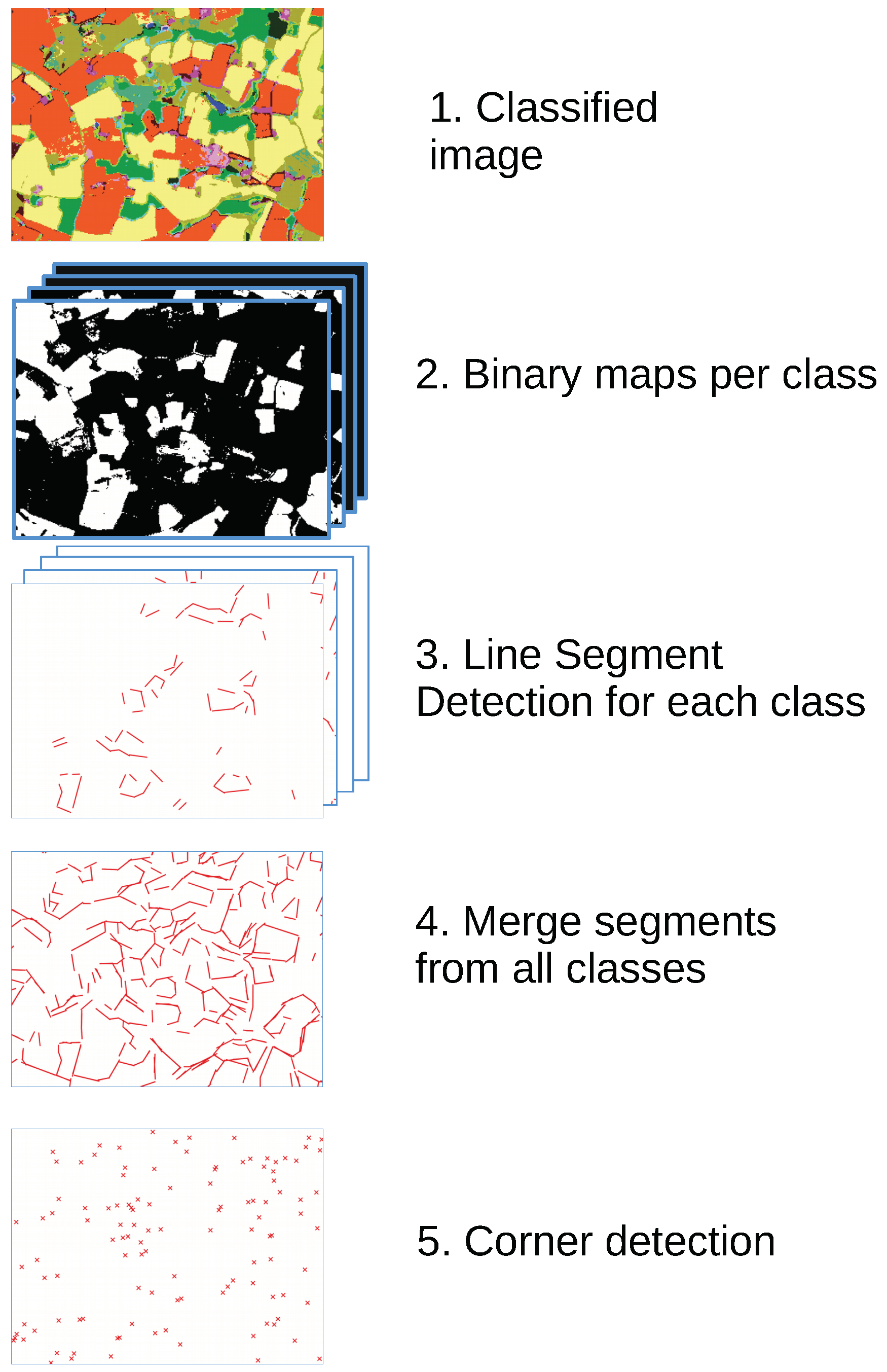
2.1. Corner Detection

Detecting the corners in a classification map can be done by extracting straight line segments in the map, and by calculating the position and angle of the intersection between pairs of lines. For this, first of all, the classification map is split into a set binary maps (one binary map for each class). Then, an unsupervised Line Segment Detector (LSD), based on [29], is applied to the map, generating a set of segments for each class. In order to find corners on the edges of areas of various classes, all of the segments of the different classes are merged together. A corner is detected if the angle of the two segments is within a certain range (30°–120°), and if their extremities are close enough. This is shown in Figure 2.

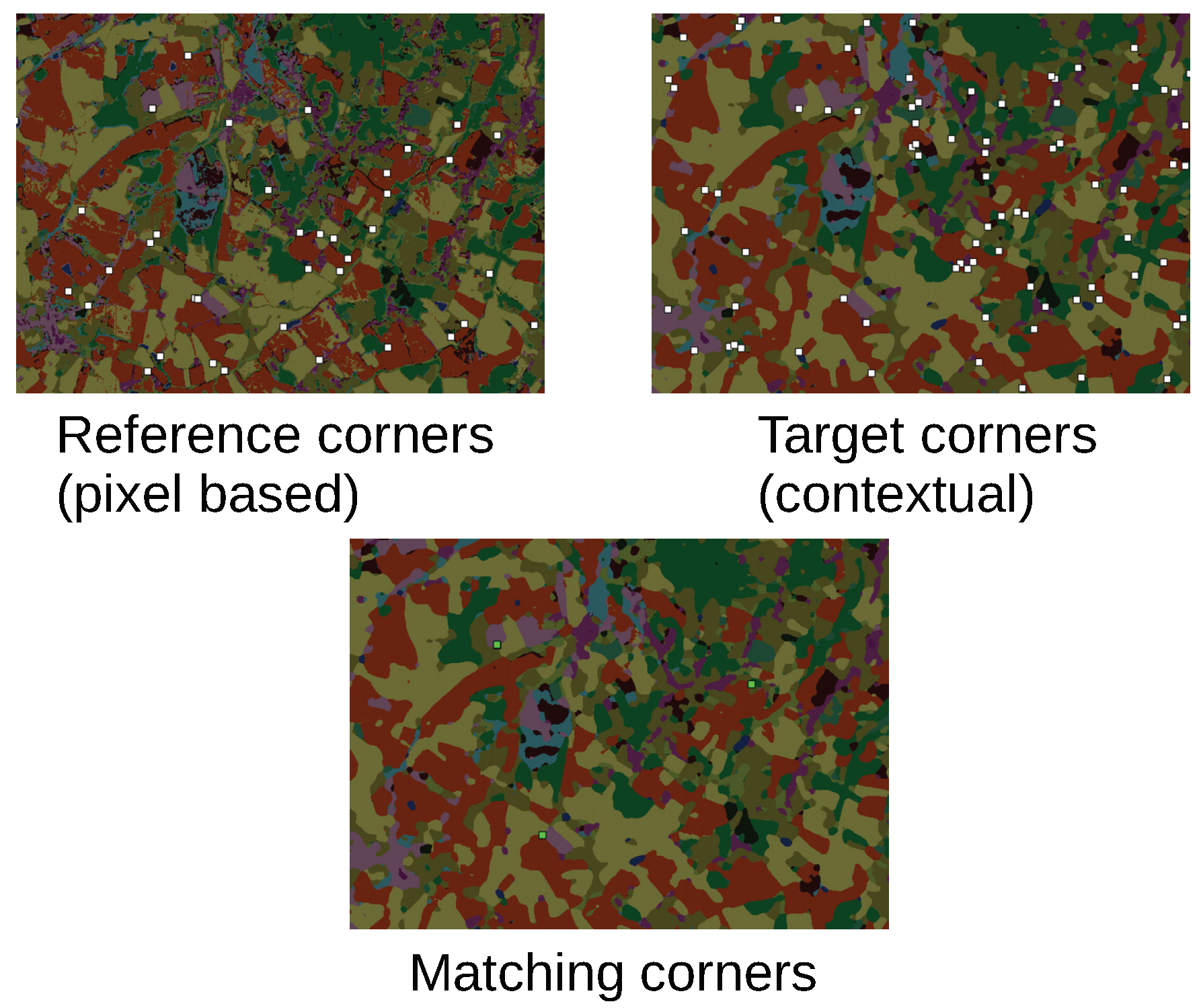
2.2. Corner Matching

After the corners have been extracted in both the target classification map and the reference classification map, the ratio of corners that match up in both maps to the number of corners in the target classification is used as a performance metric. In other words, let C r e f be the set of corners of the reference image (the pixel-based classification), and C t e s t be the set of corners of the classification map of which geometry is being measured. The set of matching corners is defined in Equation (1), where d i s t ( x , y ) is the standard Euclidean distance, and t is a threshold parameter. This is also illustrated in Figure 3.
C m a t c h = { x C t e s t y C r e f , d i s t ( x , y ) t }
From here, the geometric precision metric P B C M can be defined, as is shown in Equation (2).
P B C M = C a r d ( C m a t c h ) C a r d ( C t e s t )
A high ratio means that many of the corners detected in the target are also present in the pixel-based classification, and reversely, a low ratio means than many of the corners in the pixel-based classification have been lost. When comparing two pixel-based classifications generated with a different sampling of training data, and therefore a different Random Forest, an average matching ratio of 51.3% is measured, see Figure 5. This seemingly low number is due to imperfections in line and corner detection, which are sensitive to the label noise present in the pixel-based classification.
In order to increase the robustness of the metric, each target classification can be compared to several pixel-based results, which are generated by classifiers trained on various random samplings of the training data. This reduces the contribution of noise, in the same manner as a cross-validation scheme. Then, the average value and standard deviation of the metric can be calculated, in order to provide an indication of the confidence of the metric, when different sub-samplings of the training data are used.
The PBCM metric also has its limits, as it only measures the smoothing of corners, and not of other high spatial resolution features, such as fine elements. Furthermore, it is biased by the corners of the majority classes, in this case, the two crop classes (summer and winter crops), which account for the wide majority of corners detected in these maps. The geometry of other classes, such as the urban classes, which are unfortunately the most challenging to classify, might not be measured in this case. The metric might also overlook the geometry of minority classes, which do not generate many corners in the first place. However, it still can play the role of an indicative metric, as these biases are known and can be accounted for in the interpretation. Moreover, it would be possible to add weights to the different corners, according to the classes that form them, and in this way to reduce the biases linked to class proportions. However, this would be application dependent and is not developed further in this work.

2.3. Impact of Regularization

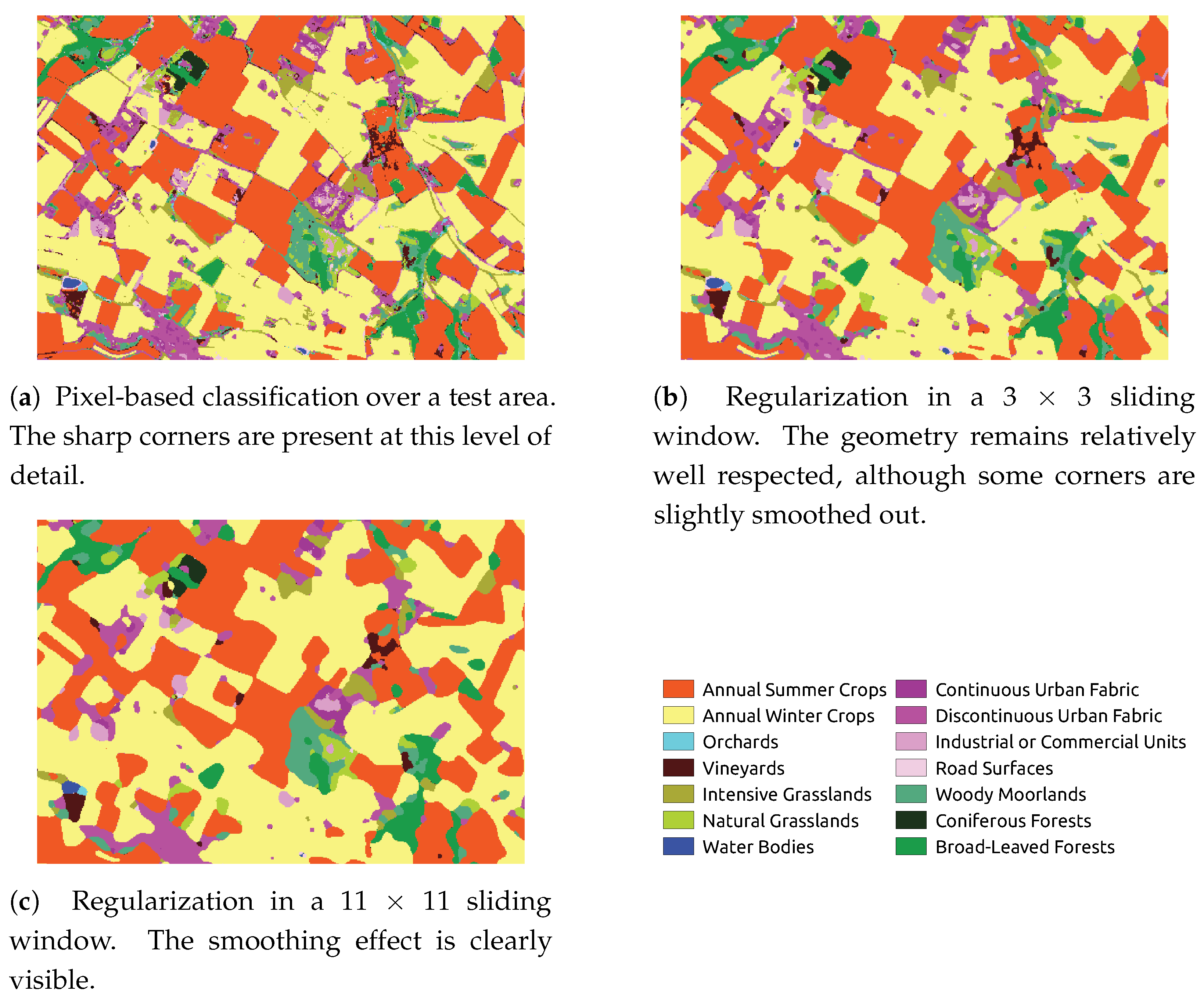
To demonstrate the pertinence of the metric, a majority vote filter, also known as regularization filter, is applied in a sliding window to the result of a pixel-based classification. This common post-processing step consists in replacing the label of the central pixel of the sliding window by the most frequent label in the neighborhood. It is known to increase the statistical accuracy by removing isolated pixels in the final result. This is illustrated in Figure 4. Figure 4a shows the result of a pixel-based classification, which contains sharp corners, and a certain amount of isolated pixels, that can be attributed to noise. As Figure 4b demonstrates, this noise is largely reduced by the regularization filter. However, the corners are slightly smoothed. In Figure 4c, a larger neighborhood of 11 × 11 pixels was chosen for the regularization filter, which has a heavy smoothing effect on the previously sharp corners.
The impact of the regularization on the statistical accuracy is shown in Figure 5. In this figure, the vertical axis shows the difference in Overall Accuracy with respect to the pixel-based classification, while the horizontal axis represents the PBCM. The labels above the points indicate the size of the sliding window, in pixels. Clearly, regularizing the classification result using a sliding window has a positive impact on the classification accuracy metric (Overall Accuracy). This remains true, even for very large sliding window sizes. In fact, the most accurate performances are achieved for the large windows (11 × 11, 13 × 13, 15 × 15), where the geometric deformation is very visible, as is shown in Figure 4c. Figure 5 also shows that when applying a majority vote filter in a sliding window neighborhood, like in Figure 4b, the PBCM decreases as the size of the filter increases. Indeed, the metric reaches 30% for a window of 5 × 5, and passes under 10% for a window of 11 × 11. These results give a first indication that the corner matching metric is indeed sensitive to a deterioration of the geometric quality, and allows for an initial quantitative evaluation of this effect. This also shows that measuring the Overall Accuracy or the Kappa alone is not sufficient to fully evaluate the quality of a map, and that a specific metric for evaluating the quality of the geometry is indeed necessary.

2.4. Calibration of the Metric

Extracting the corners involves several parameters that need to be calibrated to the type of imagery used. In particular, the Line Segment Detector depends on 7 parameters, which all have a significant influence on how well the line segments are extracted. The advised parameters given in [29] have been selected for computer vision problems, and do not always provide coherent results when applied on binary maps at a 10 m resolution. Indeed, at such a resolution, each desired segment is made up of a relatively small number of pixels, when compared to computer vision images. Secondly, the contrast along the lines in binary maps is stronger than in natural images. For this reason, a calibration step is used before applying the metric. This involves maximizing the average number of matching corners between pairs of pixel-based classification maps, while minimizing the number of matching corners between a pixel-based classification map and a regularized classification map. In practice, the difference between the two is used as a cost function for a grid search optimization over the parameters, around their default values. Pixel-based results from several samplings of the training data are used to increase the robustness of the PBCM metric at each step of the calibration. The resulting values of the calibration are given in Table 1 and Table 2.

3. Spatial Supports

This section provides the precise definition of the three spatial supports studied in [27] and in this paper, as well as various other works that have used them, and a brief discussion on a few of the advantages and disadvantages of each one. Figure 6 shows an illustration of the three different spatial support shapes, over an agricultural area and over a textured urban area.

3.1. Sliding Windows

Many popular contextual features are based on the use of one or more sliding windows as spatial supports. These features can be basic local image statistics such as mean and variance that are evaluated in this study, and defined in Section 4. More complex descriptors such as the aforementioned Haralick texture features [6], wavelet based textures [24], or Gaussian Pyramid features [30] are also commonly used [7,8]. However, the descriptors cited above generate a very large number of features, making them difficult to use on multi-spectral time series. Indeed, classification in very high dimensional spaces is known to present certain difficulties. This phenomenon, the so called “curse of dimensionality”, can be linked to the sparsity of training data points in very high dimensional spaces [31]. The training points are insufficient to properly model the high dimensional probability density distribution of the classes, which leads to a poor classification. In addition, a very large number of features implies heavy memory and computational requirements, which are already high due to the size of multi-spectral time series.
Contextual information can also be included in a sliding window spatial support via Markov Random Fields [32,33,34,35] or Conditional Random Fields [36]. Here, the objective is to extract a model of the probabilities of the various pixel combinations, which allows for local dependencies, particularly textures, to be taken into account. However, these methods make strong assumptions on the probability density functions, which are difficult to extend to very high dimensional spaces. Random Fields are also difficult to scale, as a global energy function must be recalculated on the entire image at each iteration, at least with the most common solvers.
Finally, the most popular approach nowadays is the use of Convolutional Neural Networks. Originally designed for classifying small patches of images, these have been extended for the dense classification problems such as land cover. In [12,14,16], the authors note a deterioration in high spatial frequency areas, such as rounding, or the smoothing of small image elements, which might be linked to the absence of dense training data.
The general downside of using a sliding window as spatial support is that it has a tendency to smooth out sharp corners and to erase fine elements in the image, as its shape is not adaptive to the content of the image. Pixels belonging to sharp corners or fine elements are mainly surrounded by pixels from very different classes. For example, a pixel belonging to sharp corner, like the pixel in the corner of the field in Figure 6, is partially surrounded by elements belonging to a different class. As these pixels are all included in the spatial support, their contribution to the contextual information may overshadow the contribution from the target class, which might lead to a misclassification. Sharp corners and fine elements do not contain many pixels, but they are in fact very important, as they define the fine details of the geometry of the classification map, which provides a visually accurate result for the end user. Another way of understanding this smoothing phenomenon is to consider the spatial frequencies present in the image. Sharp corners and fine elements are linked to the high spatial frequencies of the image, and may therefore be sensitive to low-pass filtering, for instance, by using a sliding window with an averaging feature.

3.2. Object Based Methods

Due to the smoothing of high spatial frequency areas, other methods attempt to define a spatial support that is adaptive to the strong gradients in the image. The underlying objective is to preserve the geometry of the objects in the image, by considering that a spatial support should be formed by pixels that are not only nearby in the image, but also similar in terms of features.
This is the base of a popular paradigm for including contextual information: Object Based Image Analysis (OBIA) [17], which has several practical applications in remote sensing classification problems. This method makes use of image segmentation, which is the process of splitting an image in non-overlapping regions, called segments, that attempt to optimize feature homogeneity and sometimes a shape criterion. In the remainder of this paper, segments from a segmentation method like the ones commonly used in OBIA, such as Mean Shift [37] and Region Merging [38], are referred to as object segments, object neighborhoods, or objects, in reference to Object Based Image Analysis, and in contrast with superpixel segments that are defined in Section 3.3. In most OBIA approaches, object segments serve as spatial supports for calculating contextual features. If a hierarchy of segmentations is used, such methods can also include information from several scales, as is done in [23]. Furthermore, most OBIA methods make use of the spatial characteristics of the segments, i.e., their shape, size, perimeter, and other such descriptors. These features add a level of spatial information that can help in describing the context. This is shown to have a positive impact on the classification accuracy on various remote sensing problems [18,19].
However, such methods may have difficulty in characterizing highly textured areas, due to over-segmentation. Indeed, the most common image segmentation algorithms generate segments that adhere to the strong gradients in the image, but do not necessarily include diverse pixels, as the primary objective of these methods is feature homogeneity in the segments. An illustration of a Mean Shift segmentation on a Sentinel-2 image, given in Figure 7b, and the illustration of various spatial support shapes, Figure 6 show that in urban areas, object segmentation methods often isolate individual houses, streets and gardens, rather than groups of buildings, due to the strong local gradients in these areas. However, the relevant contextual information is not contained in these segments because it is the spatial arrangement of the streets, houses and gardens that truly characterizes the urban density. Generally speaking, it is the diversity of pixels and their spatial arrangement that provide a meaningful characterization of the context.
It is worth noting that all of the spectral bands and dates are used to obtain this segmentation. Segmentation on such large images can be difficult, but it is made possible with a tile-based scaling method [39].
In fact, there is usually a trade-off to be made between the adaptability of a spatial support and its ability to include diverse pixels. Sliding windows can be placed at one end of the spectrum, as they allow the inclusion of diverse pixels but are not at all adaptive to strong gradients in the image. On the other end are segments from an object segmentation method, which are very adaptive, but do not allow the inclusion of diverse pixels.

3.3. Superpixel Support

There is another type of segmentation, known as superpixel segmentation, which aims to extract spectrally homogeneous regions, but that includes another constraint: the segments should all have similar sizes, and should be equally distributed throughout the image [20]. These objectives are attained through the addition of strong size and compactness constraints to the segments during the optimization process. This implies that the average size of the superpixels can be simply controlled, as it is an entry parameter to the algorithm. Superpixels can be seen as an intermediate representation between sliding windows and object segments, because they are adaptive to strong gradients, but include a variety of different pixels in highly textured areas, due to the size constraints. Another interesting property is that when using superpixels, all of the segments have a similar size, which means that the contextual features at each scale are comparable to each other, in terms of the extent of the scale that they have considered. Feature comparability is a desirable property for classification.
The algorithm used in this study is an extension to the Simple Linear Iterative Clustering (SLIC) [20]. It uses a tile-based memory management scheme in order to apply the algorithm to images of any size, while guaranteeing an identical segmentation quality [40]. SLIC was chosen among other superpixel algorithms, because of the execution speed of the algorithm, even in very large dimensional spaces, which is necessary in order to deal with the volume of multi-spectral time series data. Figure 7a shows an extract of a SLIC segmentation applied to a 11,000 × 11,000 Sentinel-2 image time series, containing 33 images with 10 spectral bands each, covering the entire year of 2016. Cloud detection and gap-filling are applied to the image stack, as is done in [5]. The segmentation was applied on all 33 dates, but the background image shown in Figure 7 shows the RGB bands of the first date. The natural boundaries between objects are relatively well respected, and the segments are indeed all compact and similar in size. Figure 7b also shows a mean shift segmentation of the same area, with a spatial radius of 6, and a spectral radius of 500. While the fields are no longer over-segmented, the segments in the urban area are very small and do not include spectrally diverse pixels. This shows that object-based methods have difficulty segmenting out semantically relevant objects in textured areas.

4. Choice of Features

In this study, three types of contextual features are used, in order to show the impact of the shape of the spatial support in various situations. Figure 8 shows the RGB bands of two of the 33 dates of the Sentinel-2 time series over a selected area, for comparison with the contextual features given in Figure 9 and Figure 10.

4.1. Local Statistics

The first features that are considered are the sample mean and variance, calculated in the spatial support. Consider that each spatial support, which can be a sliding window, superpixel, or object, contains N k pixels, where k serves as an index for the spatial support. N k is constant for sliding windows, but can vary for superpixels or objects. Each pixel also contains D features, which in our case represent the spectral reflectances at different dates. Defining each pixel as p n d , with n [ 1 N k ] and d [ 1 D ] , the mean M k d and variance V k d of a spatial support k can be written as in Equations (3) and (4). These features were chosen because of their simplicity, but also because they can represent some aspects of a context, such as typical behavior in the spatial support, as well as the overall pixel heterogeneity. Illustrations of these two features on the RGB bands of the first date of the time series are given in Figure 9.
M k d = n = 1 N k p n d N k
V k d = n = 1 N k ( M k d - p n d ) 2 N k - 1

4.2. Edge Density

The second feature that was considered in this study is the edge density, as developed in [41]. It is calculated as the average magnitude of the 3 × 3 gradient in a given neighborhood. For multi-variate data, the edge density is calculated separately for each band, providing a number of edge density features equal to the original number of features in the image. It provides a structured measurement of the local variations, giving an indication on the roughness of the surface texture, averaged over all directions. The 3 × 3 gradient is shown in Figure 10a, and then Figure 10b–d respectively give an illustration of the edge density, i.e., the average of the magnitude, calculated in a sliding window, a superpixel, and a Mean Shift object, on the RGB bands of the first date of the time series. The superpixel and object supports seem to provide a feature with relevant values, even near object edges. In the experiments, the edge densities are calculated on each band and at every date of the time series, and are all used as features.

4.3. Shape Features

One of the advantages of OBIA is being able to exploit the shape of the segments given by the segmentation [17]. One very common way of doing so is to include features such as the compactness, area, or the squareness. An more exhaustive list of possible shape features is given in [42]. In this study, two simple shape features were selected. The perimeter-based compactness, defined in Equation (5), describes how close the perimeter to area ratio is to that of a circle. In the formula, a and p respectively designate the area and the perimeter. The area and the perimeter themselves are also used as features. These three features provide information on whether or not the segment has a compact shape, and its overall size. This feature seems more pertinent for object supports than for superpixel supports, because the latter are similarly sized, and have a relatively compact shape. Nevertheless, these features are used even when the support is a superpixel, in order to use a maximum of information for the classification, and to provide a fair comparison between object and superpixel methods.
C p = 4 π a p 2

5. Experimental Setup

For the evaluation, the benchmark problem is the 17-class land cover mapping of Sentinel-2 time series, as described in [
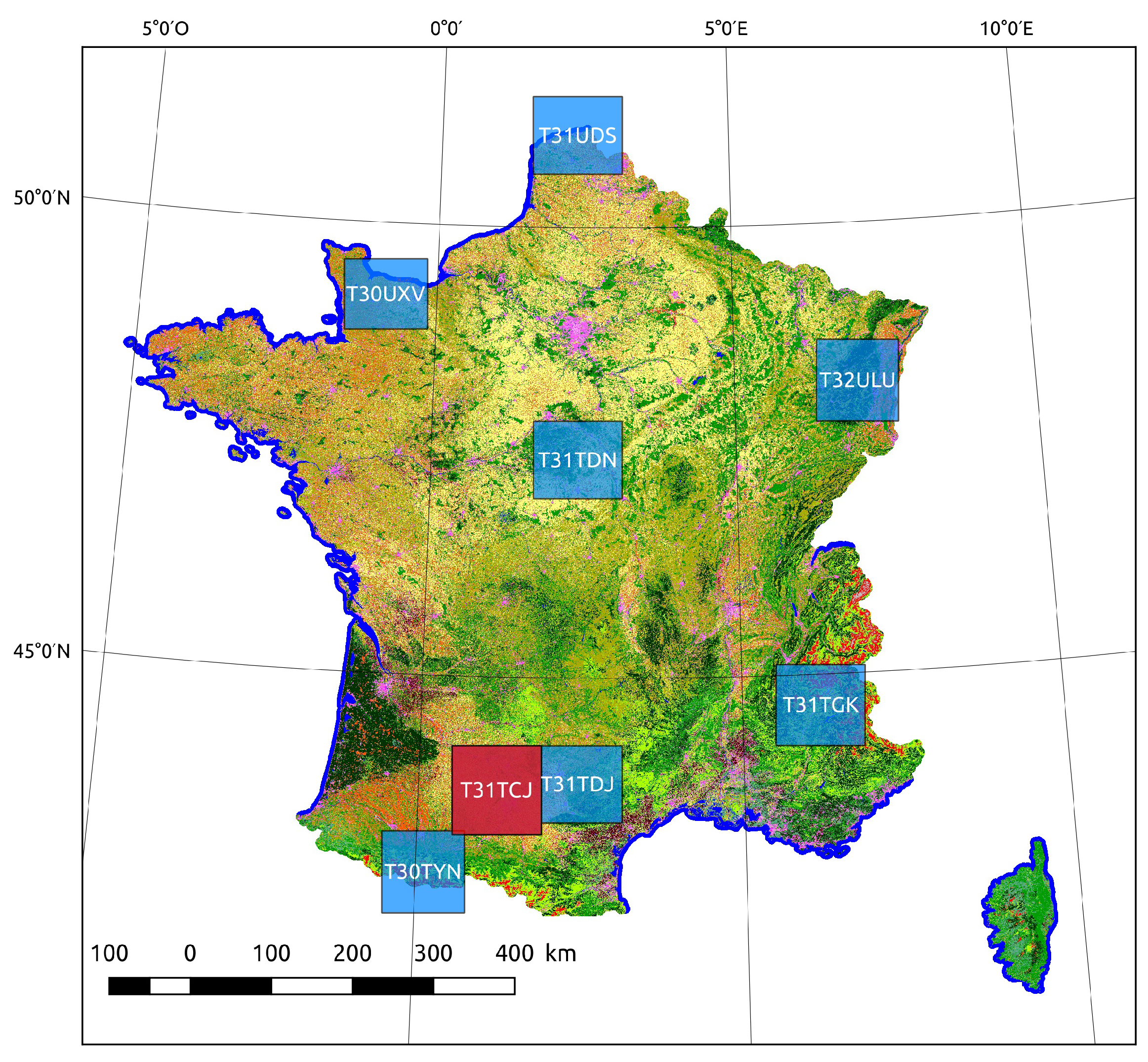
5]. The data set is comprised of 33 dates of 10 band optical images at a 10 m spatial resolution. A total of 7 different tiles of 110 × 110 km covering a variety of landscapes across France were chosen for the evaluation. The different tiles and their geographic layout is shown in Figure 11, and the number of training samples taken for each tile is shown in Table 3. Each tile contains quite different class proportions. Most illustrations and detailed analysis are based on the tile T31TCJ, which contains the city of Toulouse.
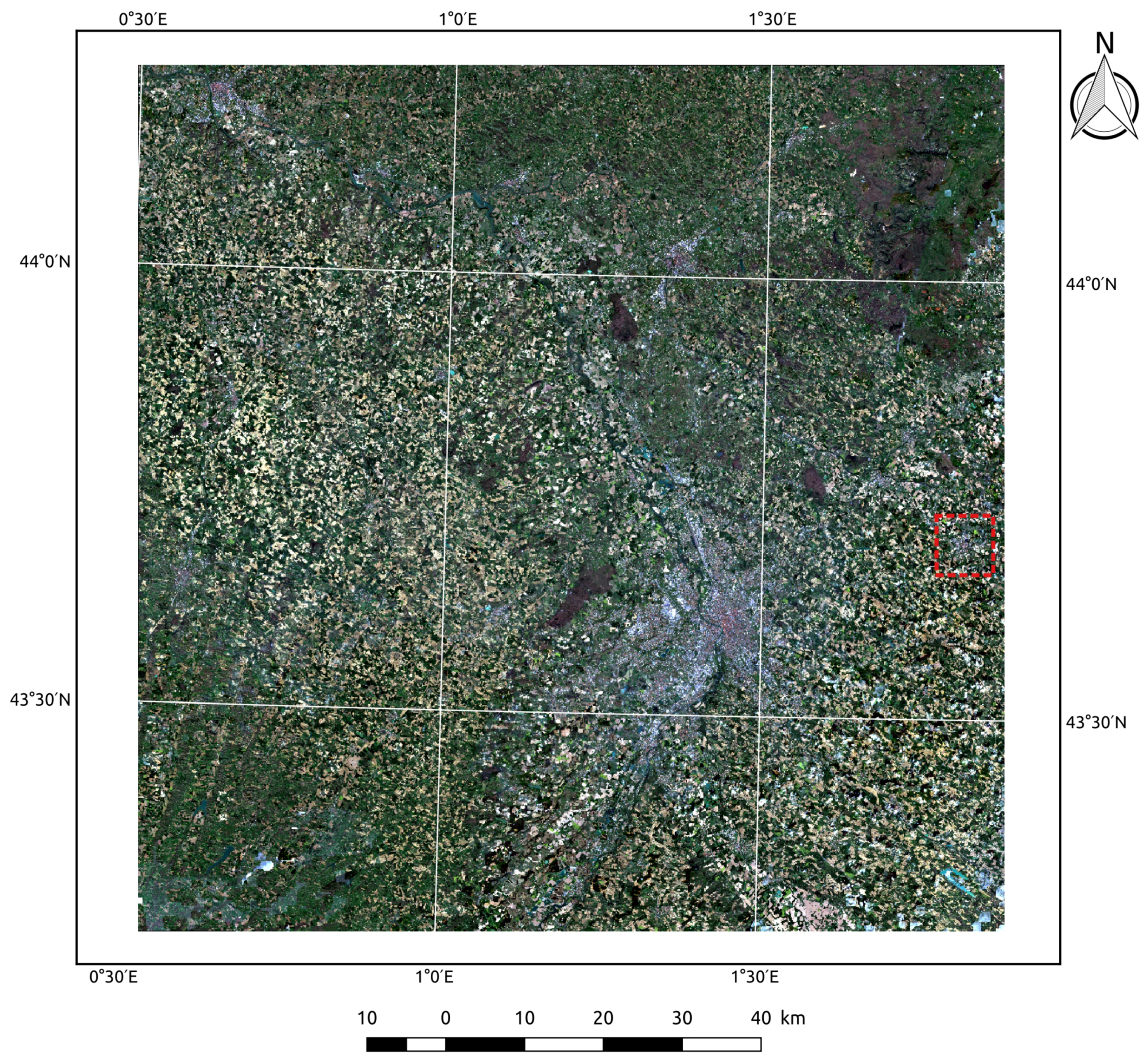
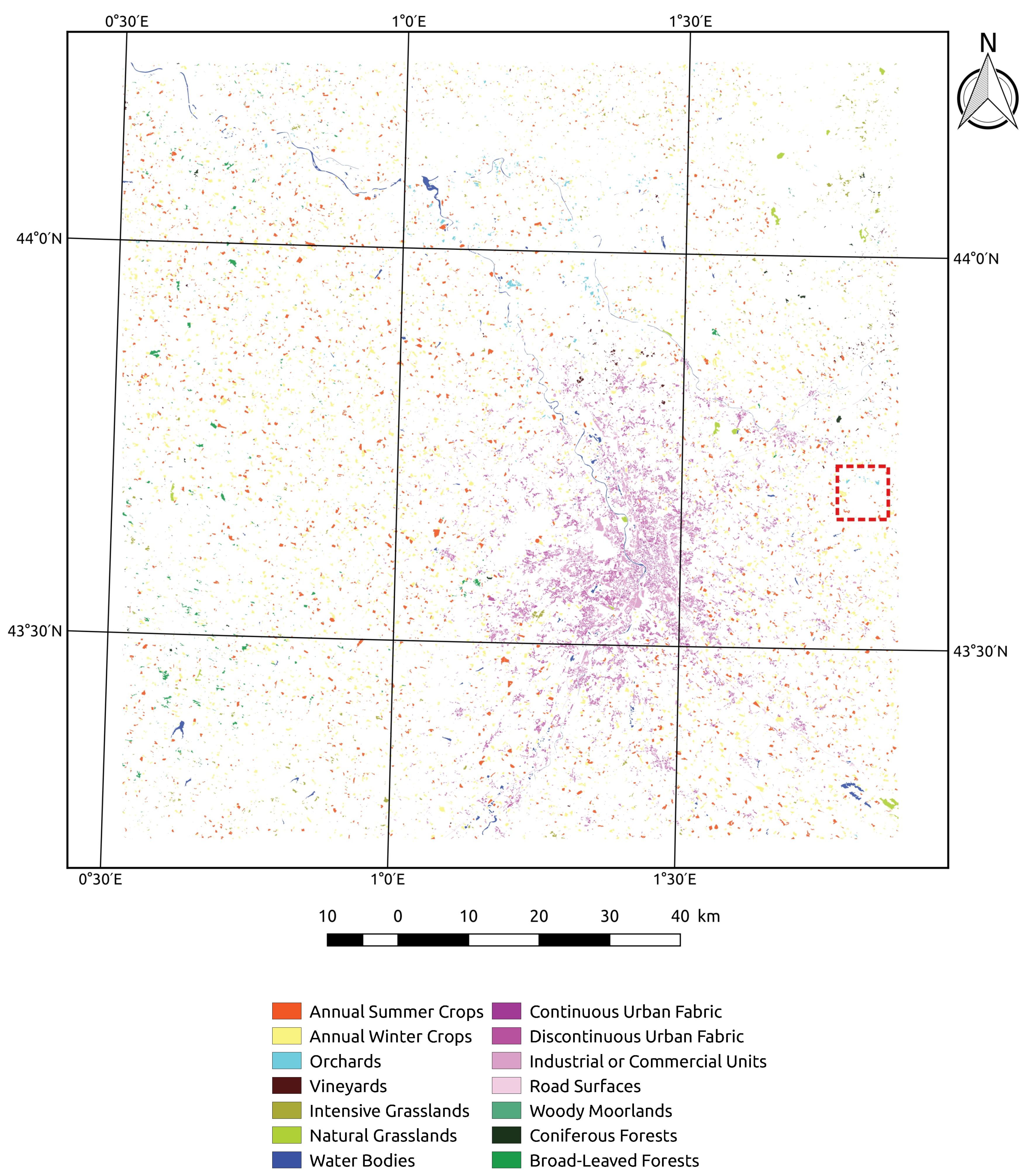
 Figure 12 and Figure 13 respectively show the RGB bands of the first date of the time series, over this area, as well as the reference data used for the training and validation of these experiments. Results for all 8 tiles in Section 6. The classifier used for the evaluation is a Random Forest [11] with 100 trees, and a maximal depth of 25.
This region was chosen among the others as it covers a wide area, including large urban agglomerations as well as a variety of forests and agricultural lands. Figure 14a shows a small area of this data set. Three spectral indices, namely the Normalized Differential Vegetation Index (NDVI), the Normalized Differential Water Index (NDWI) and Brightness, are also calculated from these images, which gives the full time series a total dimension of 489 features. A detailed description of the training data is also given in [5]. In the selected region, the nomenclature contains 14 classes, which range from agricultural classes such as summer or winter crops, to natural covers like forests and water, as well as artificial surfaces, roads and urban areas, as shown in Figure 14b. For the evaluation, the reference data is split into training and testing sets, at the polygon level, to avoid correlation between the two data sets, and to provide measurement of the generalization error, as is recommended by [43]. Each data set is comprised of 15,000 samples per class, except for the Natural Grasslands class, where around 10,000 samples are selected, as there are fewer samples available for this class. The same number of samples was chosen for the testing sets. The benchmark classification is the pixel-based Random Forest classification [11], an example the of benchmark result is given in Figure 14b.
The performance of the different methods is evaluated by the following criteria.
  • The standard classification quality metrics: Overall Accuracy, Kappa, and F-scores of classes.
  • PBCM: The quality of the geometric precision of the classification result, based on corner extraction in the binary classification maps, compared to a pixel-based classification, as explained in Section 2.
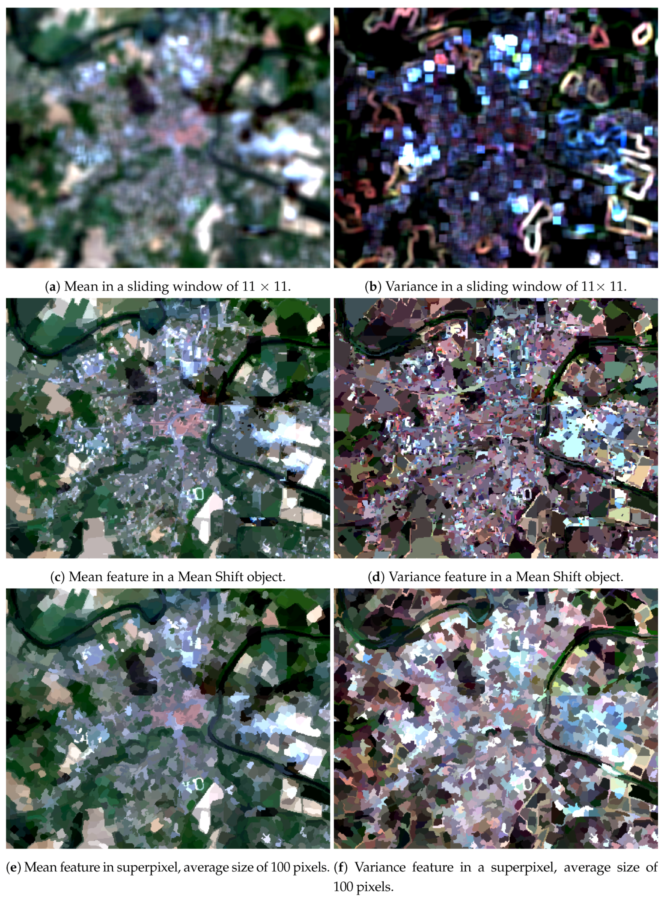
The experiments are run on two sets of features, the mean/variance features, and the edge density features. In each case, the object shape information is included if it is pertinent to the spatial support, so for objects and superpixels.
The performance of the baseline classification method, the pixel-based Random Forest classifier is given in the first column of Table 4, in Section 6.

6. Results

The experimental results are obtained by including contextual features calculated in a spatial support around the pixel that is being classified. This can be either a sliding window, a superpixel, or an object. First, a detailed analysis of the results on the tile T31TCJ is provided. This includes the class scores of the four main candidate methods, as well as graphs showing their Overall Accuracy and Pixel Based Corner Match. Next, the results on the other tiles are shown, which gives an indication of the performance of the various methods in different situations, each with unique class proportions and class behaviour.

6.1. Detailed Results on T31TCJ

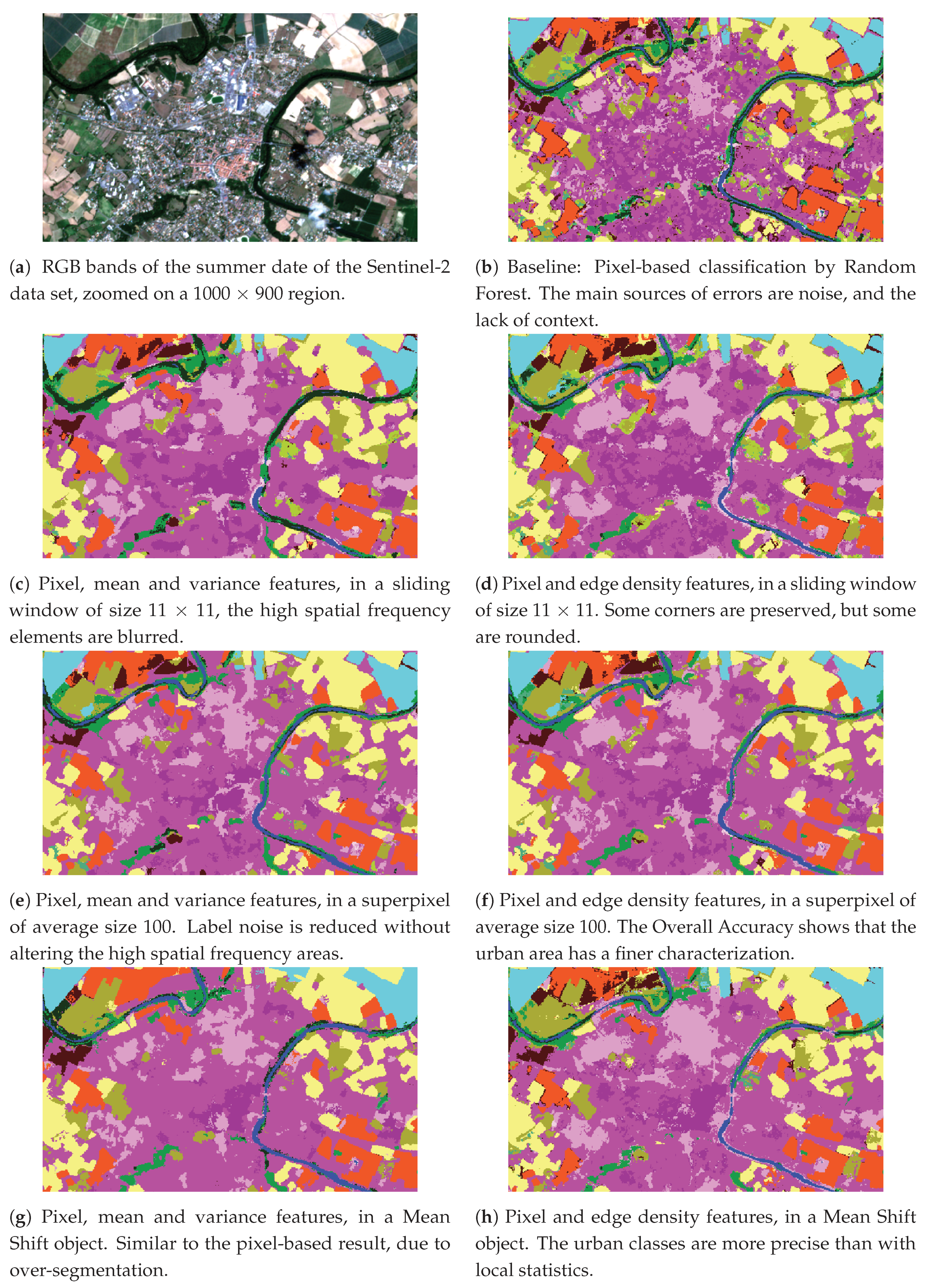
Figure 14 shows an extract of the classification maps, generated with different combinations of spatial support shape and feature choice, on an urban area with a small dense center and its surroundings. In 
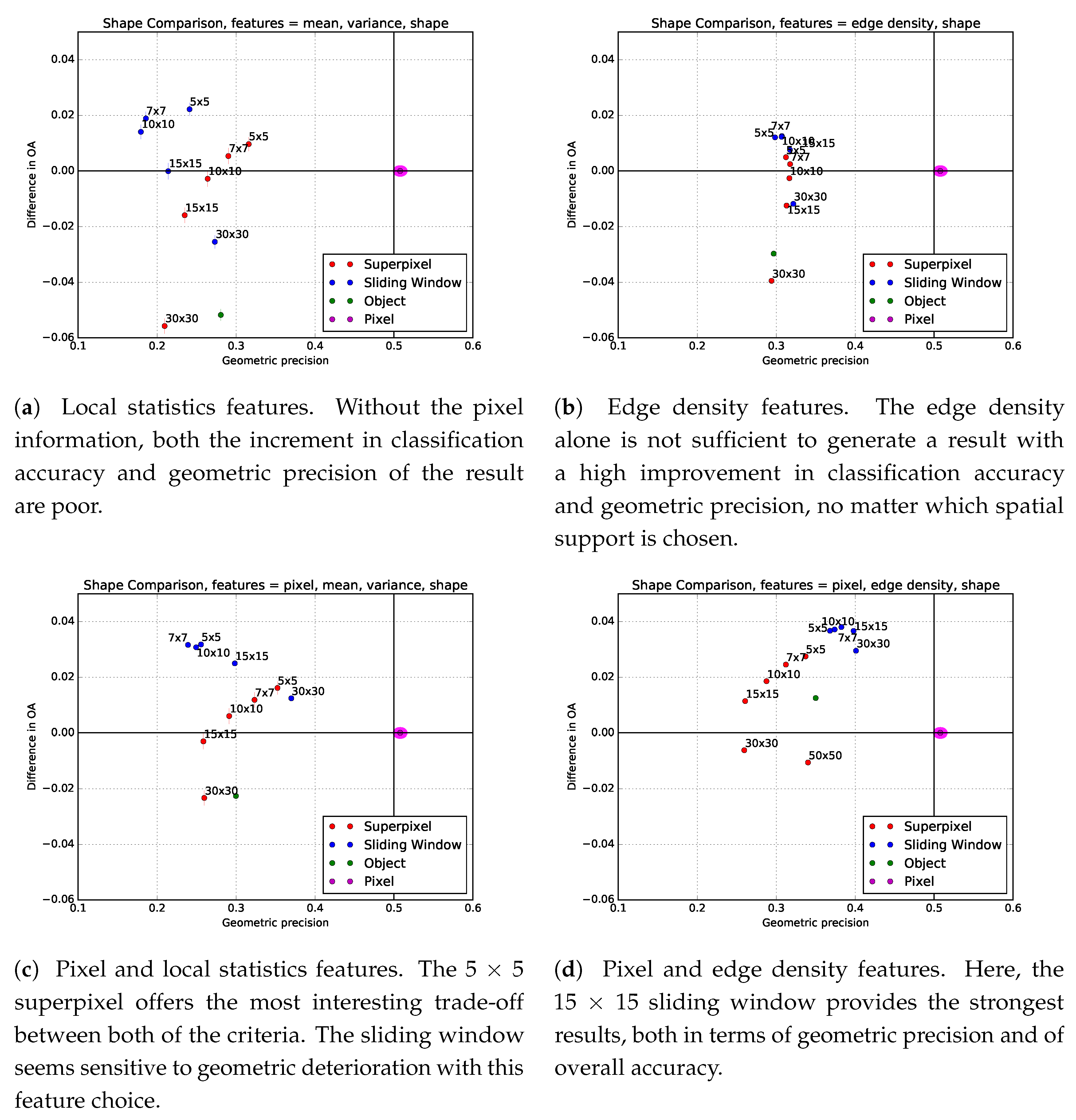
Figure 15, the different shapes and feature choices are compared according to two criteria:
  • How much overall accuracy they bring to the classification.
  • The geometric precision of the result, compared to a pixel-based classification, using the PBCM methodology described in Section 2.
The horizontal axis shows the difference between the Overall Accuracy of the contextual method and of the pixel-based method, which is also given in the second column of Table 4. The vertical axis represents the ratio of matching corners between the pixel-based classification and the contextual classification. To obtain a reference value for the pixel-based classification, the PBCM metric was calculated on pixel-based results that were generated using different sub-samples of the training set. The labels above the points represent the scale factor, which is the diameter of the window for a sliding window, expressed in pixels, or the square root of the average size for a superpixel.
Finally Table 4 shows the detailed per-class results for different combinations of features and spatial supports. This table shows that strong improvements are made for textured classes: the four urban classes, as well as orchards and vineyards. Only the crop classes seem to suffer from the inclusion of context, as these features are mainly irrelevant for them. However, their recognition rate remains very high.

6.1.1. Sliding Window

Figure 14c,d show the result of the classification when including respectively local statistics, and edge density features, in a sliding window neighborhood of size 11 × 11. Visually, it appears that the amount of noise is reduced, compared to the pixel-based classification result. However, in the case of the local statistics features, some of the corners seem quite rounded, and fine elements like the river are deformed, and at some places even lost. Using a structured texture feature like edge density, this effect is largely reduced. On the other hand, round-shaped artifacts appear in the urban area, due to the isotropic nature of the square neighborhood. Figure 15 confirms several of these conclusions. In particular, Figure 15c shows that the sliding window neighborhoods can provide an increase in classification accuracy, but at the cost of a deterioration of the geometric precision. Surprisingly, when the window size is very large (30 × 30), the geometric precision increases. To understand this it is necessary to analyze the Random Forest variable importance, as defined in [11]. It appears that when the window size is too large, the contextual information is mostly discarded by the classifier. This explains why when increasing the window size, the geometric precision increases, but the statistical accuracy decreases, because the classification gets closer to the pixel-based prediction. Furthermore, Figure 15a,b show that both the classification accuracy and geometric precision of the sliding window neighborhood result are quite low when the pixel information is not included. Finally, Figure 15d shows that using edge density features in combination with pixel features provides the best results, both in terms of classification accuracy and geometry.

6.1.2. Mean Shift Object

The result using features calculated in a object from a Mean Shift segmentation is shown in Figure 14g. The high-frequency elements are conserved, but the noise smoothing effect in the urban area is clearly less present than when using superpixels. This is due to the fact that segmentation methods like Mean Shift create very small segments in urban areas, because of the high spectral variability. Calculating contextual features in objects does therefore not bring much information when compared to pixel-based classification. This is confirmed by Figure 15a,d, as the increment in classification accuracy is quite limited, regardless of the feature choice.

6.1.3. Superpixel

When using superpixel features with an initial segment size of 11 × 11, Figure 14e,f the noise seems filtered out and the high spatial frequency elements remain in the final result. The class edges in the urban areas have the tendency to follow the superpixel edges, which adhere to strong gradients in the image. Figure 15 shows that when using a superpixel as a spatial support, the pixel-based information once again has a positive effect, increasing both the classification accuracy and geometric precision. Furthermore, with the local statistics features, Figure 15a,c, superpixels offer the best trade-off between the two evaluation criteria, although the optimal superpixel size is 5 × 5, which shows that this choice of feature and support is only relevant at smaller scales, for capturing a local context. When using the edge density and pixel information, the increase in overall accuracy is positive, and the PBCM is decent, but they remain slightly lower than when using sliding windows.

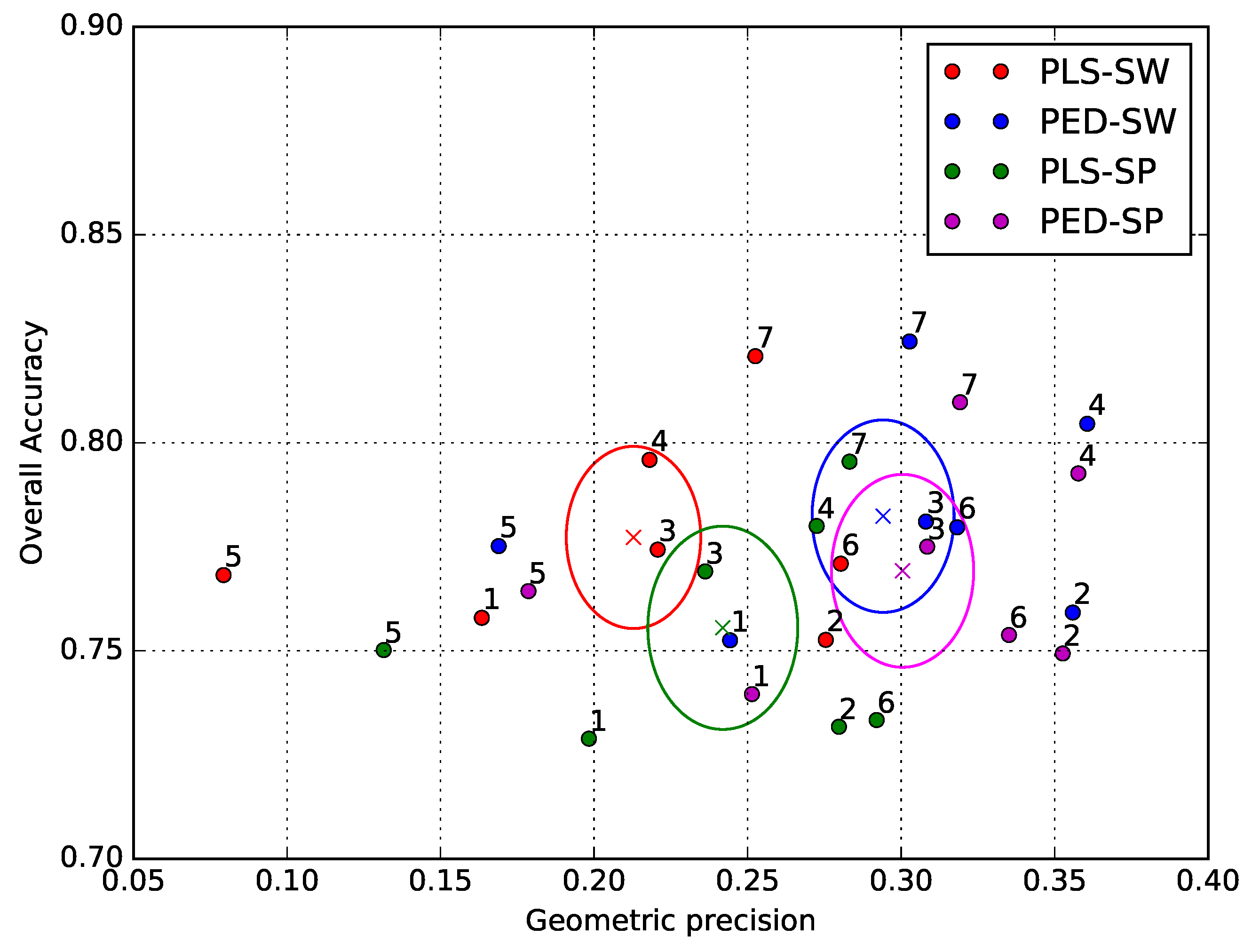
6.2. Results on Other Tiles

Figure 16 shows the Overall Accuracy and geometric precision scores for the 7 tiles present in the evaluation data set. Each point represents the performance on one tile. The scores show some variability, due to the unique class proportions of each tile. Tiles 1 and 5 (T30TYN and T30TGK) show a far lower absolute PBCM than the other tiles, no matter which method is considered. This is linked to the low number of crop classes in these tiles, which cover mountainous areas, respectively, the Alps and the Pyrenees. However, the absolute value of the geometric precision metric is not very important, as it is meant to be used as a relative metric to compare different methods. The ellipses in Figure 16 show the mean and standard deviation of the scores, over all 7 tiles. The center of the ellipse is placed on the mean value, while the length of the semi-minor and semi-major axes are equal to the standard deviation of the two scores.
The graph shows that the edge density feature systematically gives a higher geometric precision, for both superpixels and sliding windows, relative to the local statistic features. While this result may seem intuitive, the PBCM metric provides quantitative evidence to this conclusion. This might be due to the fact that the edge density is a structured feature, which takes into account local variations, and not only the overall behavior in the spatial support.
It is interesting to note that the relative values of the scores for a given method are relatively similar from one tile to another. This shows that the relative geometric precision metric is quite robust to diversity in tile content, in other words, it provides a reliable indication of the geometric degradation of a contextual classification method.
In terms of Overall Accuracy, the sliding window seems to provide the highest performance, especially in combination with the edge density feature. However, the difference with the superpixel spatial support is not that large, and the superpixel support seems to provide a slightly higher geometric precision.
The results show that the choice of spatial support and the choice of features cannot be made independently. Indeed, in the case of the local statistics features (mean and variance), the sliding windows have a strong tendency to deteriorate the geometry of the output map, particularly by smoothing out sharp corners and erasing fine elements. This phenomenon could be linked to the fact that the local statistics features are “unstructured”, meaning that they do not depend on the arrangement of pixels in the spatial support, and are therefore akin to a low-pass filter. It is interesting to note that these features are best combined with a superpixel support, which provides a modest improvement in classification accuracy, while maintaining a higher level of geometric precision. It is possible that the averaging nature of unstructured features implies that they run the risk of smoothing the output geometry, and therefore should be applied in combination with an image segmentation technique.
However, when using the edge density feature, the conclusion is quite different. Sliding windows provide the highest classification improvement, while generating a geometrically precise map, at least in the corners of the majority crop classes. Meanwhile, with these same features, superpixels seem to capture less valuable contextual information than sliding windows, although they also preserve the geometry, and do improve the context-dependent classes. This could be explained by the “structured” aspect of the edge density feature, which is based on the average of a local gradient, and therefore depends on the spatial arrangement of the pixels in the context, making corners and fine elements easier to characterize. This feature being more similar to a high-pass filter, is therefore adapted for use with a sliding window.
Finally, these experiments show that the presence of pixel information is key for providing maps with both a higher classification accuracy and a sharp geometry, especially when an unstructured feature like the edge density is used. Purely object-based methods like OBIA, whether they be used with superpixels or object segments from Mean Shift, provide inferior results on this problem.

7. Conclusions

In this paper, the Pixel Based Corner Match (PBCM), a new metric for measuring the geometric precision of a context-based classification map, in the absence of dense validation data, is presented. This metric uses the output of a pixel-based classification map to simulate dense validation data, under the assumption that the corners formed by the edges between different classes are relatively well respected by the pixel-based classifier. By matching these corners with the corners in the contextual classification map, the degradation of these high spatial frequency elements can be quantified. Experiments using regularization (majority vote in a sliding window) show that this metric provides a quantitative indication of the amount of smoothing and loss of corners that occurs when using such a post-processing step. Indeed, when increasing the size of the regularization window, the metric decreases significantly. However, it is important to keep in mind that this metric is far from perfect, as it only measures the degradation of corners, and not of fine elements. Secondly, it is strongly biased by the classes that contain the most corners, in this study, the summer and winter crops.
The PBCM metric is used to demonstrate the ability of three different spatial supports (superpixel, sliding window, and object) to improve class recognition at a 10m spatial resolution, while maintaining a precise geometry. This experimental study serves as a demonstration of how the metric can guide the choice of spatial support and features to use. Two types of contextual features, the second order local statistics (mean and variance), and the density of edges are also compared, to understand how the choice of spatial support and contextual feature can be linked.
For this land cover mapping problem, the most viable solution (in terms of both statistical and geometrical accuracy) among those evaluated here seems to be the combination of pixel features with the edge density, calculated in a sliding window. On the other hand, superpixels provide results with a high geometric accuracy, but seem to provide a less pertinent characterization of the context than sliding windows, in this case.
In conclusion, this paper shows that the geometric precision of a classification map can be evaluated efficiently over wide areas without dense reference data. This metric is meant to be used in a multi-criteria evaluation of various contextual classification methods.
Further studies could investigate the use of a dense reference data on a small area to locally validate the metric, by comparing it to other well known dense geometrical degradation indicators, such as Hoover metrics, and category specific metrics like the ones used in [23,24]. Further improvements could also include the detection of fine elements, in order to measure the degradation in such areas. It would be equally interesting to intersect the validation data with a buffer around each corner detected on a pixel-based classification result, to provide a class-specific metric of the deterioration in the corner areas. Moreover, it could be interesting to incorporate weights to the different corners, according to the classes that form them. For instance, the weights might be inversely proportional to the class frequencies, to balance the contribution of the different classes to the metric, in case of very unbalanced class proportions.
The source code of the PBCM metric uses Orfeo ToolBox, and is freely accessible [44].

Author Contributions

D.D. is the main author of this manuscript, he designed and implemented the experimental framework and contributed to the analysis of the results. J.I. defined the requirements, overviewed the process and participated in the analysis of the results. J.M. provided important technical and methodological insights on the design.

Funding

This research was funded by Centre National d’Etudes Spatiales and ATOS under PhD grant 2714.

Conflicts of Interest

The authors declare no conflict of interest.

References

  1. Petitjean, F.; Inglada, J.; Gançarski, P. Satellite image time series analysis under time warping. IEEE Trans. Geosci. Remote Sens. 2012, 50, 3081–3095. [Google Scholar] [CrossRef]
  2. Gómez, C.; White, J.C.; Wulder, M.A. Optical remotely sensed time series data for land cover classification: A review. ISPRS J. Photogramm. Remote Sens. 2016, 116, 55–72. [Google Scholar] [CrossRef] [Green Version]
  3. Thanh Noi, P.; Kappas, M. Comparison of random forest, k-nearest neighbor, and support vector machine classifiers for land cover classification using Sentinel-2 imagery. Sensors 2018, 18, 18. [Google Scholar] [CrossRef]
  4. Griffiths, P.; Nendel, C.; Hostert, P. Intra-annual reflectance composites from Sentinel-2 and Landsat for national-scale crop and land cover mapping. Remote Sens. Environ. 2019, 220, 135–151. [Google Scholar] [CrossRef]
  5. Inglada, J.; Vincent, A.; Arias, M.; Tardy, B.; Morin, D.; Rodes, I. Operational high resolution land cover map production at the country scale using satellite image time series. Remote Sens. 2017, 9, 95. [Google Scholar] [CrossRef]
  6. Haralick, R.M. Statistical and structural approaches to texture. Proc. IEEE 1979, 67, 786–804. [Google Scholar] [CrossRef]
  7. Coburn, C.; Roberts, A.C. A multiscale texture analysis procedure for improved forest stand classification. Int. J. Remote Sens. 2004, 25, 4287–4308. [Google Scholar] [CrossRef] [Green Version]
  8. Yu, Q.; Gong, P.; Clinton, N.; Biging, G.; Kelly, M.; Schirokauer, D. Object-based detailed vegetation classification with airborne high spatial resolution remote sensing imagery. Photogramm. Eng. Remote Sens. 2006, 72, 799–811. [Google Scholar] [CrossRef]
  9. Song, B.; Li, J.; Dalla Mura, M.; Li, P.; Plaza, A.; Bioucas-Dias, J.M.; Benediktsson, J.A.; Chanussot, J. Remotely sensed image classification using sparse representations of morphological attribute profiles. IEEE Trans. Geosci. Remote Sens. 2014, 52, 5122–5136. [Google Scholar] [CrossRef]
  10. Lu, T.; Li, S.; Fang, L.; Jia, X.; Benediktsson, J.A. From Subpixel to Superpixel: A Novel Fusion Framework for Hyperspectral Image Classification. IEEE Trans. Geosci. Remote Sens. 2017, 55, 4398–4411. [Google Scholar] [CrossRef]
  11. Breiman, L. Random forests. Mach. Learn. 2001, 45, 5–32. [Google Scholar] [CrossRef]
  12. Chen, Y.; Lin, Z.; Zhao, X.; Wang, G.; Gu, Y. Deep learning-based classification of hyperspectral data. IEEE J. Sel. Top. Appl. Earth Obs. Remote Sens. 2014, 7, 2094–2107. [Google Scholar] [CrossRef]
  13. Postadjian, T.; Le Bris, A.; Sahbi, H.; Mallet, C. Investigating the Potential of Deep Neural Networks for Large-Scale Classification of Very High Resolution Satellite Images. ISPRS Ann. Photogramm. Remote Sens. Spat. Inf. Sci. 2017, IV-1/W1, 183–190. [Google Scholar] [CrossRef]
  14. Kussul, N.; Lavreniuk, M.; Skakun, S.; Shelestov, A. Deep learning classification of land cover and crop types using remote sensing data. IEEE Geosci. Remote Sens. Lett. 2017, 14, 778–782. [Google Scholar] [CrossRef]
  15. Krizhevsky, A.; Sutskever, I.; Hinton, G.E. Imagenet classification with deep convolutional neural networks. In Proceedings of the 25th International Conference on Neural Information Processing Systems, Lake Tahoe, NV, USA, 3–6 December 2012; pp. 1097–1105. [Google Scholar]
  16. Maggiori, E.; Tarabalka, Y.; Charpiat, G.; Alliez, P. Convolutional neural networks for large-scale remote-sensing image classification. IEEE Trans. Geosci. Remote Sens. 2017, 55, 645–657. [Google Scholar] [CrossRef]
  17. Blaschke, T. Object based image analysis for remote sensing. ISPRS J. Photogramm. Remote Sens. 2010, 65, 2–16. [Google Scholar] [CrossRef] [Green Version]
  18. Walker, J.; Blaschke, T. Object-based land-cover classification for the Phoenix metropolitan area: Optimization vs. transportability. Int. J. Remote Sens. 2008, 29, 2021–2040. [Google Scholar] [CrossRef]
  19. d’Oleire Oltmanns, S.; Marzolff, I.; Tiede, D.; Blaschke, T. Detection of gully-affected areas by applying object-based image analysis (OBIA) in the region of Taroudannt, Morocco. Remote Sens. 2014, 6, 8287–8309. [Google Scholar] [CrossRef]
  20. Achanta, R.; Shaji, A.; Smith, K.; Lucchi, A.; Fua, P.; Süsstrunk, S. SLIC superpixels compared to state-of-the-art superpixel methods. IEEE Trans. Pattern Anal. Mach. Intell. 2012, 34, 2274–2282. [Google Scholar] [CrossRef]
  21. Priya, T.; Prasad, S.; Wu, H. Superpixels for spatially reinforced Bayesian classification of hyperspectral images. IEEE Geosci. Remote Sens. Lett. 2015, 12, 1071–1075. [Google Scholar] [CrossRef]
  22. Zhang, G.; Jia, X.; Hu, J. Superpixel-based graphical model for remote sensing image mapping. IEEE Trans. Geosci. Remote Sens. 2015, 53, 5861–5871. [Google Scholar] [CrossRef]
  23. Bruzzone, L.; Carlin, L. A multilevel context-based system for classification of very high spatial resolution images. IEEE Trans. Geosci. Remote Sens. 2006, 44, 2587–2600. [Google Scholar] [CrossRef]
  24. Huang, X.; Zhang, L.; Li, P. A multiscale feature fusion approach for classification of very high resolution satellite imagery based on wavelet transform. Int. J. Remote Sens. 2008, 29, 5923–5941. [Google Scholar] [CrossRef]
  25. Everingham, M.; Van Gool, L.; Williams, C.K.; Winn, J.; Zisserman, A. The pascal visual object classes (voc) challenge. Int. J. Comput. Vis. 2010, 88, 303–338. [Google Scholar] [CrossRef]
  26. Möller, M.; Birger, J.; Cornelia, G. Geometric Accuracy Assessment of Classified Land Use/Land Cover Changes. Photogrammetrie Fernerkundung Geoinformation 2014, 2014/2, 91–99. [Google Scholar] [CrossRef] [PubMed]
  27. Derksen, D.; Inglada, J.; Michel, J. Spatially Precise Contextual Features Based on Superpixel Neighborhoods for Land Cover Mapping with High Resolution Satellite Image Time Series. In Proceedings of the IGARSS 2018—2018 IEEE International Geoscience and Remote Sensing Symposium, Valencia, Spain, 22–27 July 2018; pp. 200–203. [Google Scholar]
  28. Pelletier, C.; Valero, S.; Inglada, J.; Champion, N.; Marais Sicre, C.; Dedieu, G. Effect of training class label noise on classification performances for land cover mapping with satellite image time series. Remote Sens. 2017, 9, 173. [Google Scholar] [CrossRef]
  29. Von Gioi, R.G.; Jakubowicz, J.; Morel, J.M.; Randall, G. LSD: A line segment detector. Image Process. Line 2012, 2, 35–55. [Google Scholar] [CrossRef]
  30. Binaghi, E.; Gallo, I.; Pepe, M. A cognitive pyramid for contextual classification of remote sensing images. IEEE Trans. Geosci. Remote Sens. 2003, 41, 2906–2922. [Google Scholar] [CrossRef]
  31. Friedman, J.H. On bias, variance, 0/1—loss, and the curse-of-dimensionality. Data Min. Knowl. Discov. 1997, 1, 55–77. [Google Scholar] [CrossRef]
  32. Melgani, F.; Serpico, S.B. A Markov random field approach to spatio-temporal contextual image classification. IEEE Trans. Geosci. Remote Sens. 2003, 41, 2478–2487. [Google Scholar] [CrossRef]
  33. Schindler, K. An overview and comparison of smooth labeling methods for land-cover classification. IEEE Trans. Geosci. Remote Sens. 2012, 50, 4534–4545. [Google Scholar] [CrossRef]
  34. Moser, G.; Serpico, S.B. Combining support vector machines and Markov random fields in an integrated framework for contextual image classification. IEEE Trans. Geosci. Remote Sens. 2013, 51, 2734–2752. [Google Scholar] [CrossRef]
  35. Kang, X.; Li, S.; Benediktsson, J.A. Spectral–spatial hyperspectral image classification with edge-preserving filtering. IEEE Trans. Geosci. Remote Sens. 2014, 52, 2666–2677. [Google Scholar] [CrossRef]
  36. Zhao, J.; Zhong, Y.; Shu, H.; Zhang, L. High-Resolution Image Classification Integrating Spectral-Spatial-Location Cues by Conditional Random Fields. IEEE Trans. Image Process. 2016, 25, 4033–4045. [Google Scholar] [CrossRef]
  37. Comaniciu, D.; Meer, P. Mean shift: A robust approach toward feature space analysis. IEEE Trans. Pattern Anal. Mach. Intell. 2002, 24, 603–619. [Google Scholar] [CrossRef]
  38. Baatz, M. Multiresolution segmentation: An optimization approach for high quality multi-scale image segmentation. Angew. Geogr. Inf. 2000, 12–23. [Google Scholar]
  39. Lassalle, P.; Inglada, J.; Michel, J.; Grizonnet, M.; Malik, J. A scalable tile-based framework for region-merging segmentation. IEEE Trans. Geosci. Remote Sens. 2015, 53, 5473–5485. [Google Scholar] [CrossRef]
  40. Derksen, D.; Inglada, J.; Michel, J. Scaling Up SLIC Superpixels Using a Tile-Based Approach. IEEE Trans. Geosci. Remote Sens. 2019, 57, 3073–3085. [Google Scholar] [CrossRef]
  41. Trias Sanz, R. Semi-Automatic Rural Land Cover Classification. Ph.D. Thesis, Université Paris 5-René Descartes, Paris, France, 2006. [Google Scholar]
  42. Van der Werff, H.; Van der Meer, F. Shape-based classification of spectrally identical objects. ISPRS J. Photogramm. Remote Sens. 2008, 63, 251–258. [Google Scholar] [CrossRef]
  43. Liang, J.; Zhou, J.; Qian, Y.; Wen, L.; Bai, X.; Gao, Y. On the sampling strategy for evaluation of spectral-spatial methods in hyperspectral image classification. IEEE Trans. Geosci. Remote Sens. 2017, 55, 862–880. [Google Scholar] [CrossRef]
  44. Derksen, D. Source code of Pixel Based Corner Match. 2019. Available online: https://github.com/derksend/corner-matching (accessed on 15 July 2019).
Figure 1. Example of sparse reference data used for producing and validation land cover maps, shown over the RGB bands from a Sentinel-2 image in January 2016, near the city of Toulouse in southern France. Evaluating the geometry of a classification result cannot be done directly with such validation data, as it does not contain the precise boundaries between different objects.
Remotesensing 11 01929 g001
Figure 2. Corner extraction process. First, the image is split into binary maps for each class. Then, the Line Segment Detector is applied on each binary map. In order to extract corners from various classes, the segments are all merged together before the corner detection step.
Remotesensing 11 01929 g002
Figure 3. Corner matching. The corner detection is applied on a pixel-based classification, called the reference, and on a contextual classification, called the target. The PBCM is the ratio of matched corners to the number of corners in the target.
Remotesensing 11 01929 g003
Figure 4. Regularization (majority vote filtering) in increasingly large sliding windows shows the smoothing of round corners.
Remotesensing 11 01929 g004
Figure 5. Impact of the sliding window majority vote regularization on the Overall Accuracy and geometric precision (PBCM). Each pixel is assigned the majority label in the sliding window. The size of the filter, in pixels, is shown next to the points. This kind of regularization increases the statistical classification scores, however, the image of the result shows that the corners are strongly smoothed out. This is confirmed by the PBCM metric. The axes of the ellipses show the standard deviation of both the Overall Accuracy and the PBCM, over the 10 runs with different subsets of training data.
Remotesensing 11 01929 g005
Figure 6. Illustration of the three neighborhood shapes: Sliding windows, Objects, and Superpixels over two areas with different contextual characterizations.
Remotesensing 11 01929 g006
Figure 7. Different segmentations of a Sentinel-2 image time series, on a discontinuous urban fabric. Background: RGB bands of the first date.
Remotesensing 11 01929 g007
Figure 8. RGB bands of two of the 33 dates of the Sentinel-2 time series, zoomed on a 1000 × 900 area.
Remotesensing 11 01929 g008
Figure 9. Example images of the mean and variance features on the RGB bands of the first date, calculated in the three spatial support types.
Remotesensing 11 01929 g009
Figure 10. Illustration of the edge density feature in the three spatial support types.
Remotesensing 11 01929 g010
Figure 11. Extent and naming convention of the 8 Sentinel-2 tiles used in this study. These tiles cover a variety of landscapes, with very different climatic conditions, and thematic content. The tile in red (T31TCJ) is the one used in the detailed experiments of Section 6.1.
Remotesensing 11 01929 g011
Figure 12. The area chosen for the detailed experiments is 110 × 110 km tile containing the city of Toulouse in the lower right side of the image (T31TCJ in Figure 11). The image shows RGB bands of the first date of the Sentinel-2 time series. The red dotted line represents the extent of the region shown in Figure 9, Figure 10 and Figure 14.
Remotesensing 11 01929 g012
Figure 13. Reference polygons, later split into training and the validation sets.
Remotesensing 11 01929 g013
Figure 14. Results of different combinations of spatial support shapes and feature choice.
Remotesensing 11 01929 g014
Figure 15. Differences in overall classification accuracy compared to the pixel-based classifiers, plotted against the PBCM, for the different combinations of features and spatial supports. Whenever relevant, the shape features were included.
Remotesensing 11 01929 g015
Figure 16. Overall Accuracy plotted against geometric precision for the tiles numbered 1–7 in the experimental data set (see Table 3 for the equivalent tile names). P indicates the presence of pixel information, LS stands for local statistics, and ED for edge density. The centers of the ellipses, symbolized by crosses, are placed on the coordinates of the average score over the 7 tiles. The size of the ellipses represents the standard deviation.
Remotesensing 11 01929 g016
Table 1. Calibration parameters of the Line Segment Detector, as presented in [29].
S Σ q τ log ( ϵ ) DN Bins
0.80.6245°00.71024
Table 2. Calibration parameters of the corner extraction and corner matching. The angle interval and extremity distance threshold define how a corner is extracted from two segments. The angle formed by the segments must be within the interval and the extremities must be at a distance smaller than the threshold. The matching threshold determines how much tolerance is taken when matching corners from two different classification maps.
Angle IntervalExtremity Distance ThresholdMatching Threshold
60°–120°10 m (1 px)10 m (1 px)
Table 3. Number of samples taken for training on the various tiles. The number of samples is the same for the validation of the results of each tile.
Tile NameT30TYNT30UXVT31TDJT31TDNT31TGKT31UDST32ULU
Tile Index1234567
Summer crop15,00015,00015,00015,000257615,00015,000
Winter crop927115,00015,00015,00014,14915,00015,000
Broad-leaved15,00015,00015,00015,00015,00015,00015,000
Coniferous15,00014,57515,00015,00015,000154115,000
Nat. Grasslands15,000015,00073215,000137715,000
Woody Moorlands15,000797515,00015,00015,00084688641
Cont. Urban327114,1541841224737315,00015,000
Disc. Urban15,00015,00015,00015,00013,73915,00015,000
I.C.U.14,70615,00015,00015,000567915,00015,000
Roads1674230710292803121412,9009203
Beaches, dunes15,0004060015,00000
Bare Rock038110168714,31537780
Water12,51115,00015,00015,00015,00015,00015,000
Glaciers, snow197800015,00000
Intensive Grassland15,00015,00015,00015,00015,00015,00015,000
Orchards37220521718096122578695
Vineyards89015,00027847803433
Table 4. Overall and per-class accuracy (F-score), for the best feature/support combinations on the tile T31TCJ. In the feature descriptions, P indicates the presence of pixel information, while LS stands for local statistics, and ED for edge density. The bold numbers indicate the two highest values for each metric. The PBCM of these cases is also shown. The combination of sliding window, pixel and edge density provides the best results over most of the urban classes. Superpixels with pixel and edge density features provide similar values in overall accuracy, but their geometric precision seems to be inferior.
Spatial Supp. WindowWindowSuperpixelSuperpixelObjectObject
FeaturePixelP+LSP+EDP+LSP+EDP+LSP+ED
Scale 51555
Overall Acc.73.7% ± 0.2176.9% ± 0.2377.4% ± 0.2375.0% ± 0.2576.8% ± 0.2271.3% ± 0.2074.9% ± 0.13
Kappa71.7% ± 0.2775.1% ± 0.2475.6% ± 0.2573.1% ± 0.2775.0% ± 0.2469.1% ± 0.2173.0% ± 0.12
Summer crop0.9140.9020.9000.8900.8910.8910.884
Winter crop0.9090.8990.9000.8970.9000.8910.888
Broad-leaved0.8310.8310.8430.8120.8410.8040.837
Coniferous0.8060.8190.8410.7980.8320.7920.822
Nat. Grass.0.3220.3500.3430.3230.3400.1720.218
Woody Moor.0.4730.4810.4690.4590.4740.3410.418
Cont. Urban0.6040.6870.6780.6220.6630.6290.636
Disc. Urban0.5760.6580.6900.6310.6710.5030.641
I.C.U.0.5920.6710.6900.6420.6710.5990.652
Roads0.8380.8820.8990.8560.8800.8060.857
Water0.9890.9900.9890.9880.9880.9890.988
Int. Grass.0.6770.6930.6960.6780.6980.6760.662
Orchards0.8240.8590.8570.8630.8640.8410.863
Vineyards0.8330.8680.8550.8630.8640.7950.846
PBCM51.3% ± 0.9625.6% ± 1.1438.26% ± 0.5534.43% ± 0.433.06% ± 0.3829.6% ± 0.3135.6% ± 0.46

