Article

Monitoring Tropical Forest Structure Using SAR Tomography at L- and P-Band

1
National Research Institute of Science and Technology for Environment and Agriculture (IRSTEA), University of Montpellier, Land Environment Remote Sensing and Spatial Information (TETIS), 34090 Montpellier, France
2
National Center for Remote Sensing, National Council for Scientific Research (CNRS), Riad al Soloh, 1107 2260 Beirut, Lebanon
3
Doctoral School of Sciences and Technologies, Lebanese University (LU), 1003 Beirut, Lebanon
4
Laboratory of Informatics, Robotics, and Microelectronics of Montpellier (LIRMM), University of Montpellier, 34090 Montpellier, France
5
National Aeronautics and Space Administration (NASA), Jet Propulsion Laboratory (JPL), California Institute of Technology, Pasadena, CA 91125, USA
*
Author to whom correspondence should be addressed.
Remote Sens. 2019, 11(16), 1934; https://0-doi-org.brum.beds.ac.uk/10.3390/rs11161934
Submission received: 17 July 2019 / Revised: 14 August 2019 / Accepted: 16 August 2019 / Published: 19 August 2019

Abstract

:
Our study aims to provide a comparison of the P- and L-band TomoSAR profiles, Land Vegetation and Ice Sensor (LVIS), and discrete return LiDAR to assess the ability for TomoSAR to monitor and estimate the tropical forest structure parameters for enhanced forest management and to support biomass missions. The comparison relies on the unique UAVSAR Jet propulsion Laboratory (JPL)/NASA L-band data, P-band data acquired by ONERA airborne system (SETHI), Small Footprint LiDAR (SFL), and NASA Land, Vegetation and Ice Sensor (LVIS) LiDAR datasets acquired in 2015 and 2016 in the frame of the AfriSAR campaign. Prior to multi-baseline data processing, a phase residual correction methodology based on phase calibration via phase center double localization has been implemented to improve the phase measurements and compensate for the phase perturbations, and disturbances originated from uncertainties in allocating flight trajectories. First, the vertical structure was estimated from L- and P-band corrected Tomography SAR data measurements, then compared with the canopy height model from SFL data. After that, the SAR and LiDAR three-dimensional (3D) datasets are compared and discussed at a qualitative basis at the region of interest. The L- and P-band’s performance for canopy penetration was assessed to determine the underlying ground locations. Additionally, the 3D records for each configuration were compared with their ability to derive forest vertical structure. Finally, the vertical structure extracted from the 3D radar reflectivity from L- and P-band are compared with SFL data, resulting in a root mean square error of 3.02 m and 3.68 m, where the coefficient of determination shows a value of 0.95 and 0.93 for P- and L-band, respectively. The results demonstrate that TomoSAR holds promise for a scientific basis in forest management activities.

1. Introduction

Tropical Forests play a vital role in the global carbon cycle, and subsequently within the global climate [1]. Tropical forests are incredibly complicated, diverse, and frequently threatened. Indeed, there’s a crucial demand to develop a new technology to help in surveying and revealing the dynamics of tropical forests. The dynamic processes like growth, regeneration, decay, and disturbance, strongly affects the forest 3D structure. Forest 3D structure is so closely associated with their history, diversity, function, and micro-climate [2]. At the same time, forest structure information is essential for developing a precise forest biomass estimators. The latter is needed to observe better and evaluate forest ecosystems’ contribution in the overall carbon cycle [3,4,5]. Traditionally, forest structure observation has been implemented by inventory plots at local scales. Inventory measurements provide correct estimates of a variety of single trees and stand parameters. However, these measurements are time demanding and they are performed at smaller scales. The extrapolation of those plot measurements from into larger scales depends on the ability of these measurements to represent their surrounding landscape [6]. The establishment of the temporal continuity of these measurements is challenging. Remote sensing techniques have the potential to overcome this limitation and make an enormous contribution in qualitative and quantitative observation of three-dimensional forest structure [7,8,9,10].
Today, Tomography Synthetic Aperture Radar (TomoSAR) and airborne LiDAR are the two technologies that allow the measurement of 3D forest structure. Measures derived from the LiDAR waveform are utilized to evaluate structural forest parameters as forest height and biomass [11]. Recently, continuous forest mapping with global coverage at spatial and temporal resolutions is assessed and established using SAR imaging configuration. Indeed, a big effort has been put to demonstrate the potential of typical SAR configurations to estimate spatial biomass utilizing SAR measurements [12]. The SAR system provides measurements sensitive to the whole vegetation and from the underlying ground at high spatial resolution. The initial step started with introducing SAR interferometry as it has an exaggerated sensitivity to forest geometry and vertical structure components. Polarimetric interferometric SAR measurements allows model-based inversion to assess vertical forest structure parameters such as forest height and biomass [13,14,15,16]. The next step is using multi-baseline interferometric acquisitions in order to reconstruct the vertical distribution of the scatterers [17]. Recently, tomographic acquisitions, which will be seen as an extension of multi-baseline interferometric acquisitions, have been used to reconstruct the three-dimensional radar reflectivity of forests [17,18,19,20,21,22,23]. The promising outcomes accomplished initiated the execution of TomoSAR acquisition modes in future spaceborne SAR missions, like Biomass [24] or Tandem-L [25], for mapping structural forest parameters and to enhance the performance of biomass estimators at a global scale.
TomoSAR has been demonstrated to be a powerful tool for observing forested areas from space owing to its capability in providing vertical resolution based on multi-baseline observations [17,26,27,28]. Tomographic techniques consist of power estimation strategies applied to the multi-baseline Single Look Complex (SLC) data to retrieve the back-scattered power that characterizes the vertical profile of forests [29,30]. In its most simple formulation, TomoSAR aims to extract the vertical distribution of the backscattered power within the system resolution cell. A potential answer to the current problem is to take advantage of super-resolution techniques like Capon beamforming, Multiple Signal Classification, Singular Value Decomposition analysis, and others [26,31]. A unique solution could also be found within the works by Fornaro et al. [32] and Cloude [33,34], wherever super-resolution is achieved by exploiting prior information concerning target location, like ground topography and canopy height model [34]. The capabilities of L-band TomoSAR to characterize 3D vertical structure of tropical forests are still in early stages of development while those of P-band TomoSAR have been discussed and evaluated. Ho Tong Minh et al. [35] used the airborne data that were acquired during TropiSAR campaign to prove that the use of L-band tomographic imaging in tropical forests seems limited. The first experience in testing TomoSAR in tropical forest areas was carried out in French Guiana by the TropiSAR campaign in 2009. However, these data were sub-optimal to assess the performance of multi-frequency TomoSAR in monitoring the forest structure and estimating forest structure parameters as forest top height. To overcome such limitation, and acquire optimal tomographic and polarimetric data, the AfriSAR campaign was successfully carried out over the dense forests of Gabon in 2015 and 2016. Nevertheless, the link between physical forest structure and the reconstructed 3D radar reflectivity is still not understood and is far from being established. The main challenge, thus, is the interpretation of 3D radar reflectivity in terms of the 3D forest structure parameters.
The 3D radar reflectivity relies on the operating system frequency and polarization. Plus, it also depends on the used acquisition geometry (e.g., incidence angle), and the achieved 3D spatial resolution. In fact, the generic interpretation of 3D reflectivity is difficult because scatters that are seen by radar are changing with frequency and polarization. Accordingly, this paper focuses mainly on comparing the capabilities of L- and P-band TomoSAR to extract forest top height. First, the P- and L-band vertical profiles are validated with a Canopy Height Model (CHM), which is obtained from a Small Footprint LiDAR (SFL) dataset. Second, qualitative comparisons of the Capon beamforming profile at HH and HV (H: horizontal, V: vertical) polarizations with Land Vegetation Ice Sensor (LVIS) Level 1B waveform LiDAR data and CHM and Digital Terrain Model (DTM) from SFL data, over the region of interest in Gabon Lopé National Park, are carried out. Additionally, forest top height is retrieved from the TomoSAR data.
The paper is organized as follows: Section 2 describes the study area, datasets, and methods used for the tomographic analysis. Section 3 illustrates the validation of the results. Section 4 is devoted to discuss and interpret the tomography results. Section 5 demonstrates the concluding remarks.

2. Materials and Methods
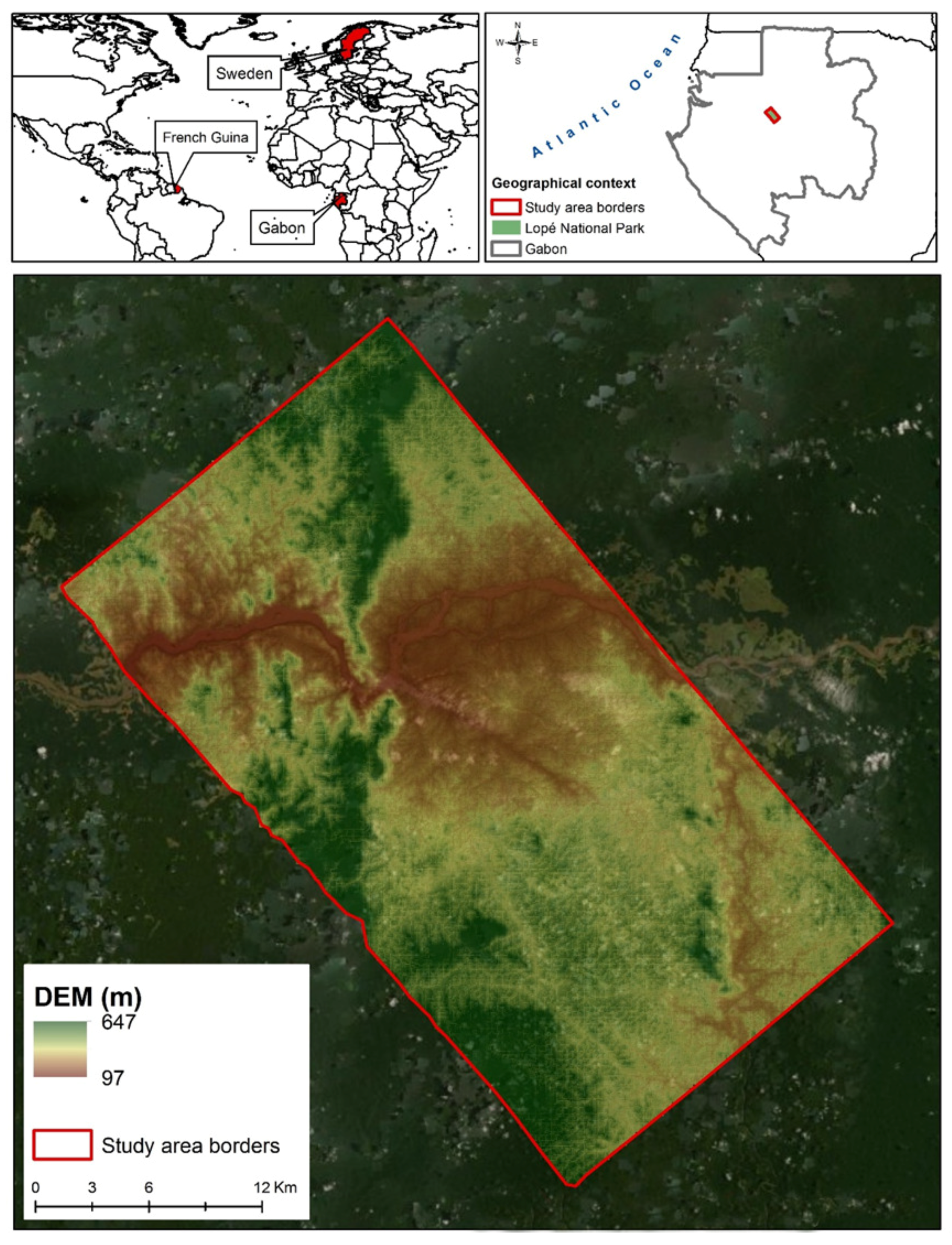
2.1. Study Area

To develop algorithms that assess the performance of BIOMASS SAR measurements in different forest ecosystems, several airborne field campaigns have been designed and implemented. One can name the AfriSAR campaign in Gabon, BioSAR campaign in Sweden, and TropiSAR campaign in French Guiana (Figure 1).
The AfriSAR campaign aims to provide support to forthcoming NISAR, GEDI and BIOMASS missions. Four sites presenting various forest structures have been selected: Lopé, Mabounie, Mondah, and Rabi, located, respectively, at 250 km, 180 km, 25 km, and 260 km from the Libreville airport, where the calibration site was deployed. In this section, we will focus on the presentation of Lopé, which is the primary acquisition site. Lopé National Park, a 4913 km2 national park in central Gabon, is known as one of the largest parks in the area. The scene of the northern part consists of the last remnants of grass savanna that was created in central Africa, during the ice age from 15,000 years ago. This natural site is composed of vast areas of Savanna in the north, which is surrounded by the Ogooué River and frequently burned in order to preserve the forests’ Savanna areas, in addition to an extended area of tropical forests that are combined with parts of successive forests of complex structure, which were developed throughout time with savanna recolonization [36]. Lopé is a convenient natural view to prove the adequate performance of tomographic imaging because of the gradient of forest biomass from the forests’ savanna boundary (up to 100 Mg/ha), to dense undisturbed humid tropical forests (greater than 400 Mg/ha). The height and structure of the trees vary gradually from savanna into forests, which provide uniform mono-dominant trees of okoume (OKO) of tall: 30–50 m for regions with the presence of significant gaps in mid-canopy. This creates skewed vertical profiles. Lopé topography is also diverse. It varies between either broad flat plains or steep sloping terrains. OKO2 region is selected to perform a qualitative analysis between UAVSAR–TomoSAR L-band, SETHI P-band vertical profile, and LiDAR waveforms.

2.2. Data-Set

During the AfriSAR campaign, different datasets have been acquired over the Gabon Lopé National Park. The NASA sponsored AfriSAR campaign involved three data sets, L-band UAVSAR data, LVIS LiDAR data, and SFL data. ONERA and DLR defined a common configuration for P-band imaging of their radar systems. P-band SAR P-band acquisitions were performed by ONERA (SETHI radar system) in July 2015 and by DLR (F-SAR radar system) in February 2016.

2.2.1. LiDAR Data-Sets

Throughout the AfriSAR campaign, the SFL data set was collected by the NASA Jet Propulsion Laboratory (JPL) in July 2015, with a footprint diameter of 10 cm. Canopy Height Model (CHM) and Digital Terrain Model (DTM) rasters are provided with 1 m spatial resolution. The second LiDAR dataset was collected in March 2016, NASA’s Land Vegetation Ice Sensor (LVIS) acquired the LiDAR data set as part of NASA–ESA’s BIOMASS, GEDI, and NISAR calibration and validation activities. LVIS is a large-scale, waveform LiDAR with applications for measuring ground elevation and vertical profile of the vegetation structure in various ecosystems. The LiDAR datasets LVIS consists of two levels: Level 1B and Level 2 (data can be downloaded from https://lvis.gsfc.nasa.gov/Data/Data_Download.html). Level 1B data contain geo-referenced LiDAR returned waveforms, such that, at each footprint, we have a corresponding shot number, and, using this shot number, one can get the LiDAR waveform at each footprint. Level 2 data contain geo-referencing data for different reflecting surfaces within the laser footprint, the locations of which were derived from the Level 1B waveform.

2.2.2. Radar Acquisition Configuration
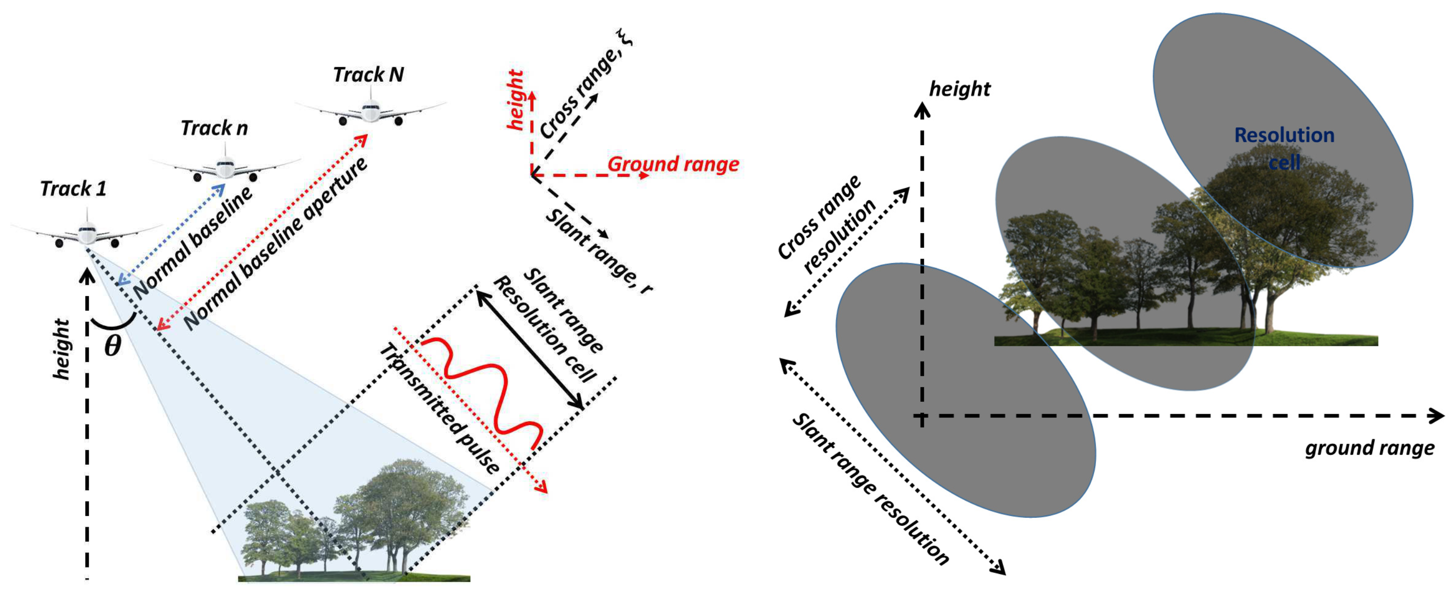
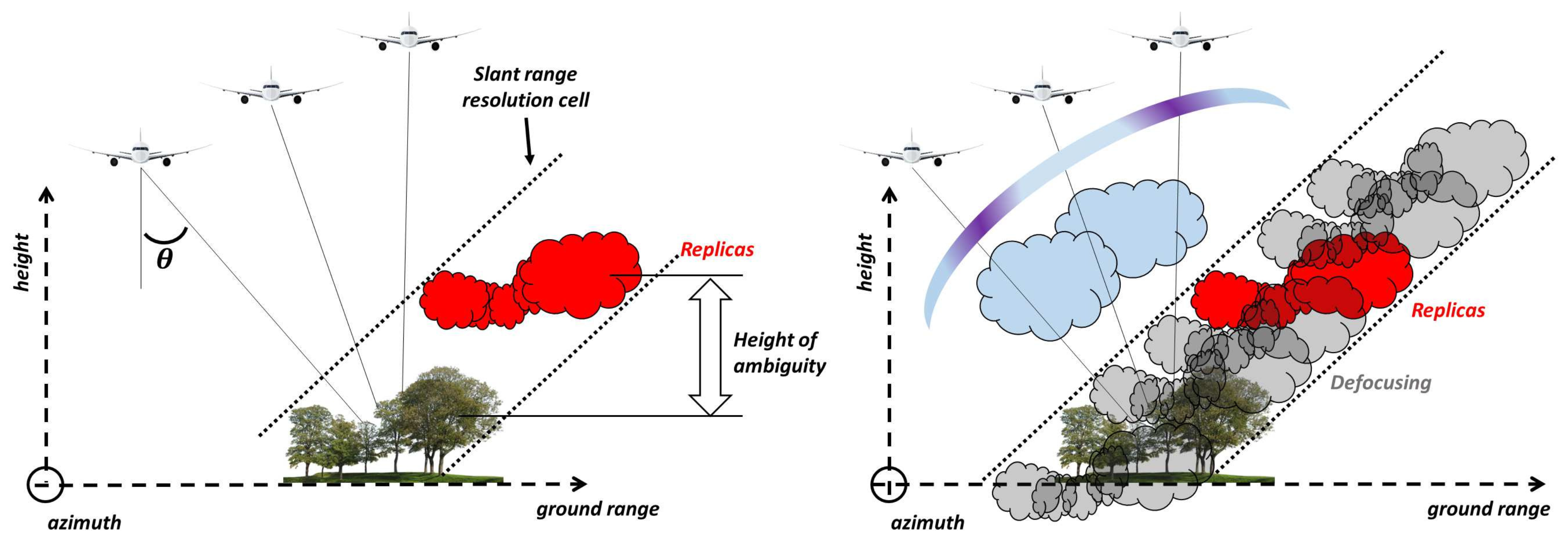
The tomographic data set here consists of seven fully polarimetric Single Look Complex (SLC) data L-band NASA/JPL UAVSAR from AfriSAR data conducted over the Lopé during the AfriSAR campaign in 2016. The operating band of UAVSAR platform is 1217.5–1297.5 MHz. The scanning of about a 22 km wide area, with incidence angles extending from 25 to 60 degrees, is performed by the Gulfstream III jet at that flight at an altitude of 12.5 km. The ground range and azimuth resolution of the UAVSAR polarimetric SLC are 1 m and 2.5 m, respectively. The tomographic SLC data acquired over Lopé by increasing the flight altitude by 20 m each flight track. The configuration of L-band UAVSAR is shown in Table 1, while the P-band data consists of 13 fully polarimetric SLC data acquired by ONERA over the Lopé in the AfriSAR airborne campaign (July 2015). The data collection is performed using the SETHI SAR system developed by ONERA and onboard a Falcon 20 aircraft. The pixel resolution of the SLC images is 1.54 m in azimuth range and 3 m in slant range. The configuration of P-band SETHI data including acquisition geometry, bandwidth, carrier frequency, and aircraft altitude are shown in Table 2.
The tomographic 125 MHz data set considered in the Paracou experimental site consists of six fully polarimetric SLC images at L and P-band acquired on 24 August 2009. All the acquisitions took about 1 h (from 9:00 a.m. to 10:00 a.m.), resulting in almost no temporal decorrelation.
In this paper, we also used six tracks fully polarimetric images acquired during TropiSAR campaign over Paracou. In the following section, we will compare P and L band tomographic results conducted over Gabon Lopé Park with the LiDAR data set SFL.

2.3. Tomography SAR

TomoSAR implementation requires accurate handling concerning the relative phase difference between different acquisitions. The rationale of TomoSAR is to use multiple flight tracks that are nearly parallel to each other [35], as shown within the left panel of Figure 2.
The ensemble of all flight lines allows the formation of 2D synthetic aperture, ensuing the coherent multiple Single Look Complex (SLC) images of various passes, providing the likelihood of focusing the signal within the entire 3D space. We will refer to (r, x, ξ ) as the slant, azimuth, and cross ranges, respectively. Consider a dataset of SLC images acquired by N parallel track sensors, denoted by Y n (r, x, ξ ), representing the SLC value inside the resolution cell (r, x, ξ ) within the n-th image. The expression of topography-compensated (tc) SLC data are often approximated [37] as:
Y n ( r , x ) t c = P ( r , x , ξ ) e x p ( j K n ξ ) d ξ ,
where P(r, x, ξ ) denotes the projection of target reflectivity on the cross-range axis ξ , and ξ represents the cross-range coordinate, orthogonal to the measuring system line-of-sight (LOS) that are outlined by the slant range coordinate. In TomoSAR applications, the vertical sensitivity of the phase difference between two acquisitions is linked through the vertical wavenumber kn expressed by:
K n = 2 π H o A = 4 π λ R b n ,
where HoA is the height of ambiguity, λ is the radar wavelength, R is the slant-range distance, and b n is the horizontal distance between the two acquisitions.

2.4. Tomography Inversion

SAR data were acquired over forests from slightly different altitude and incidence angles, providing helpful information within the vertical direction [29]. In this paper, the Capon beamforming power estimator was applied to represent the vertical profile of vegetated areas. The Capon spectral estimator is a conventional non-parametric method in tomographic analysis that enables one to obtain the endless vertical profile of the vegetation without any prior knowledge on the statistical properties of the data [38]. The Capon estimator vertical profile P c ( ξ ) is retrieved from the covariance matrix of the SLC data [26]:
P c ( ξ ) = 1 a ( ξ ) t W 1 a ( ξ ) ,
where a( ξ ) is the steering vector containing the interferometric information for a scatter at cross range ξ for all the baselines relative to a master track, and W is the maximum likelihood estimation of the covariance matrix. t is the transpose operator.

2.5. TomoSAR Phase Calibration

The previous section described the theoretical model for tomographic analysis assuming no disturbances on the path of the propagating signal. Prior to Multi-baseline SAR algorithms, the phase calibration of the TomoSAR data should be taken into account, in order to compensate the phase residuals that influence the focusing of Multi-baseline SAR data. These phase disturbances originate from atmospheric propagation delays or uncertainties in allocating the platform position.
Indeed, for airborne systems, the atmospheric perturbations are limited (no ionosphere propagation). The phase screen compensation method chosen to be applied on the Lopé data are largely inspired by the work of Tebaldini et al. [37]. A simple proposition is to assume that the phase residuals only result from uncertainties in the antennas’ positions (Figure 3). The phase screens α n can be approximated as a function of d Z n and d Y n , which represent, respectively, the position errors of the platform n in altitude and in the ground range direction for a fixed position in azimuth [37]:
α n = 4 π λ ( d Y n s i n θ + d Z n c o s θ ) .
The Double Localization iterative procedure described in detail in [37] is then put in place. The calibration is carried out by removing phase screens from the original SLC data to obtain the calibrated SLC data:
Y n c a l = Y n · e x p ( j · α n ) .

2.6. Forest Structure Parameters

The main parameter we want to estimate is forest top height. The principal challenge in tropical forests is the estimation of the forests’ top height since it is usually difficult to clearly recognize the top leaf or part of a tree in the canopy. Utilizing the Capon beamforming power estimator, we can recover the 3D backscatter profile from the multi-layer SLC and demonstrate the vertical backscatter distribution function. To do this, we applied the method proposed in [39] and we estimated the forest top height H from L- and P-band data:
H ( r , x ) = a r g m i n ( P ( H n , r , x ) P ( H c , r , x ) K ) ,
where P(Hn, r, x) is the backscatter at the phase noise level, Hn is the elevation of the noise level, K is the power loss value, and Hc is the LiDAR height value from SFL data. Since the forest top height retrieval depends on the choice of the power loss value K, we used the CHM from the SFL dataset to select the optimal power loss value. One can estimate the canopy height model from TomoSAR data by either ranging the power loss from the phase center location in the upper envelope of the Capon profile, or by ranging the power loss from the noise level (location of the highest return detected by the TomoSAR) from Hn down to the canopy contribution peak elevation in the upper envelope of the 3D profile. At each position, the Root Mean Square Error (RMSE) between the H height and Hc is calculated at given K value (H(r, x) − Hc(r, x)); once we have the lowest value of RMSE, we get the forest top height H at each (r, x) position.

3. Results

In this section, the limitation of L-band TomoSAR imaging in dense forests using TropiSAR data acquired over Paracou is illustrated; then, we report the results of forest structure characterization over Gabon Lopé National Park by means of tomography imaging using AfriSAR L- and P-band TomoSAR SLC data.

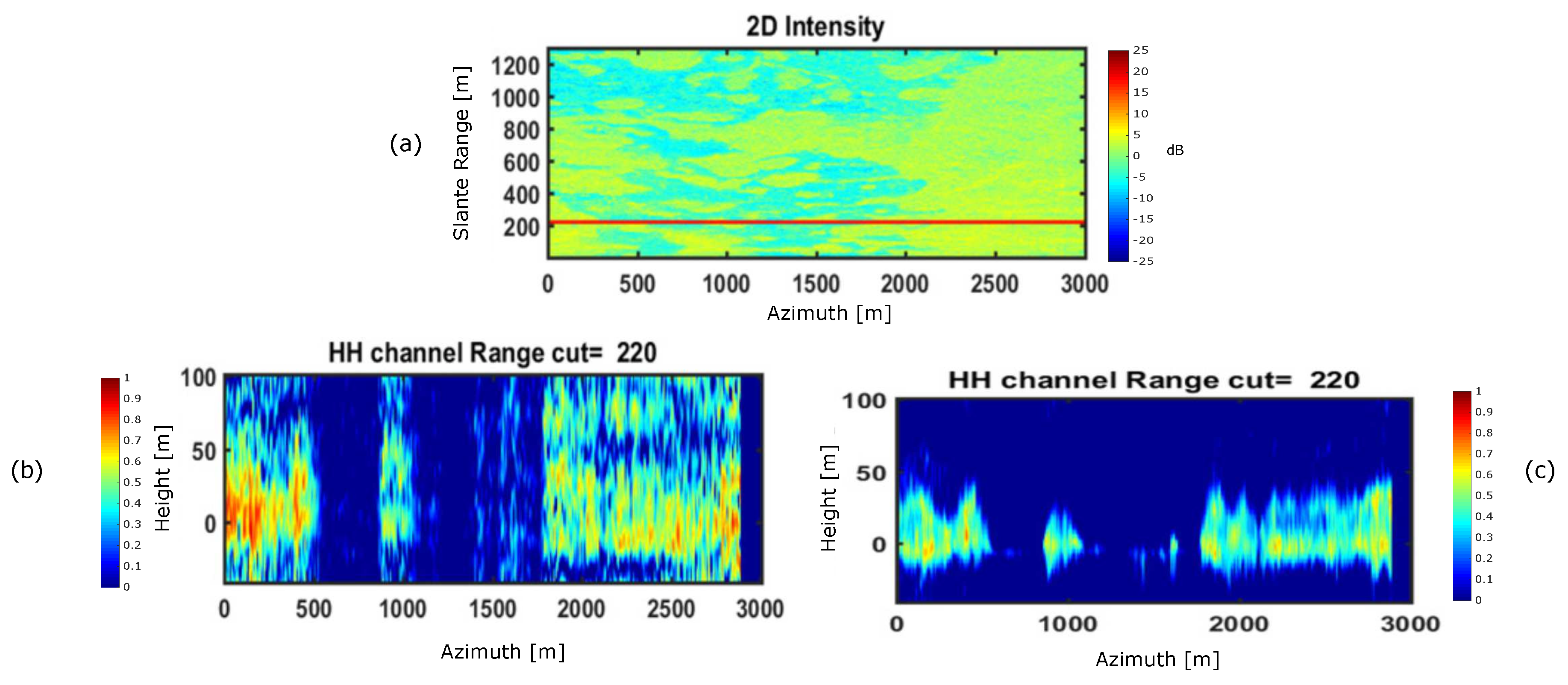
3.1. Limitation of L-Band TomoSAR in Tropical Forest (TropiSAR Data)

Figure 4 presents the tomographic profile of a constant range section at P-and L-band in tropical Paracou forest and Boreal Krycklan forest. For better visualization, the panels have been normalized in a way that the sum along the height is unitary. In the boreal Krycklan forest, the white line denotes forest top height derived from LiDAR measurements. At the tropical forest in Paracou, the L-band tomogram is not clear at all, as there is a blurring phenomenon, while, on the other hand, the P-band tomogram is clear. The different vegetation layers are illuminated correctly. However, for the Boreal Krycklan forest, the tomograms at L- and P-band are clear with no significant disturbances.

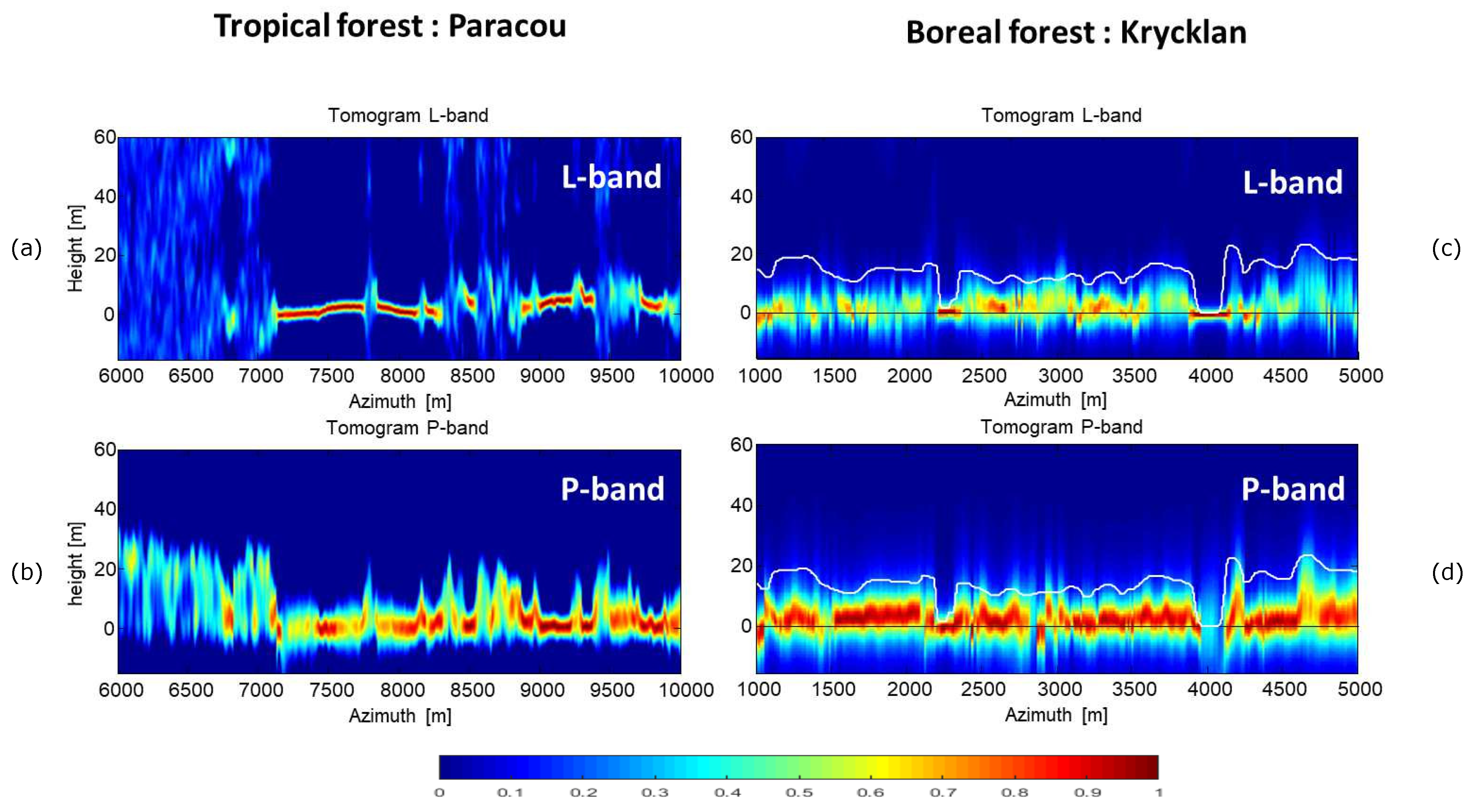
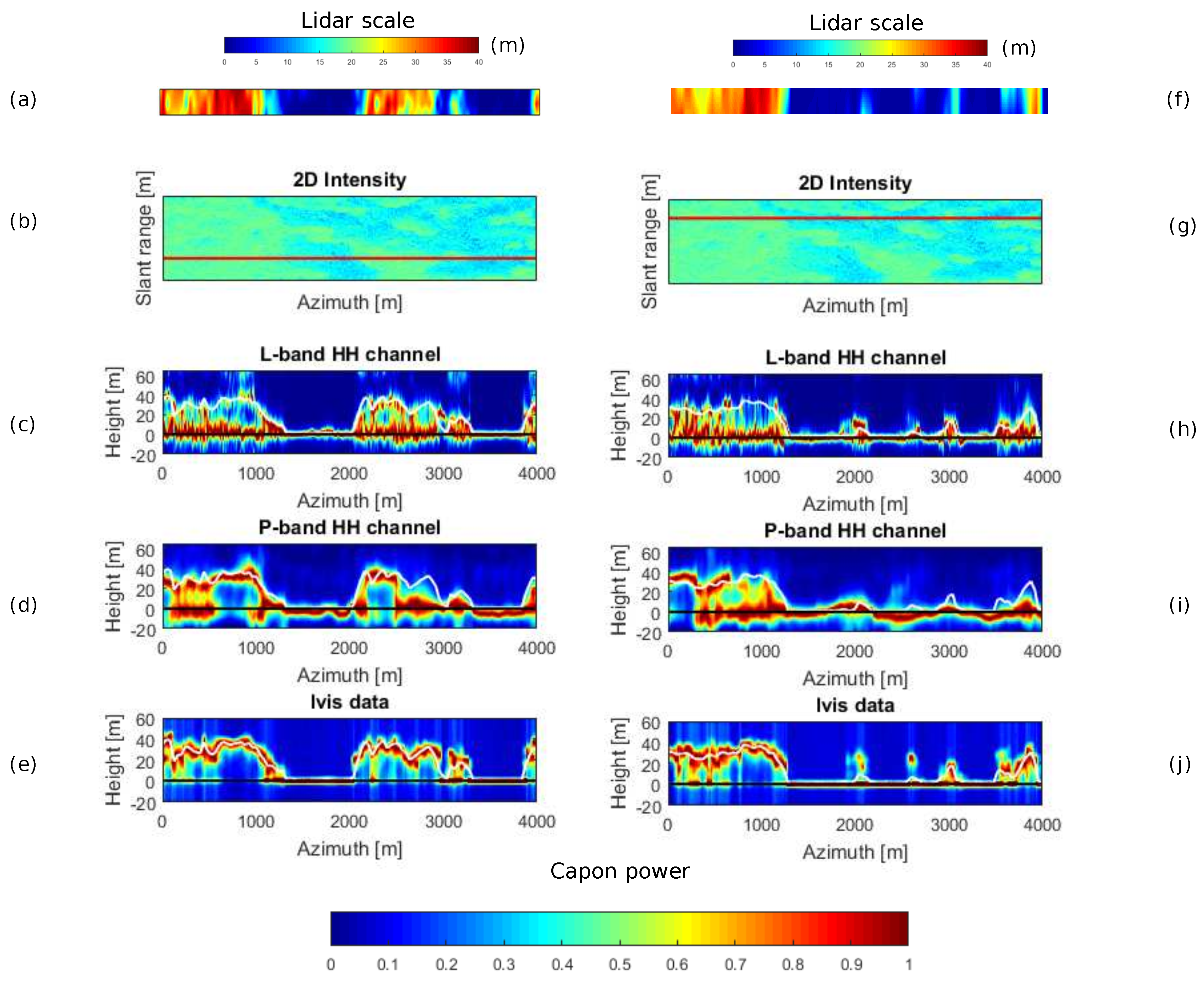
3.2. TomoSAR Profiles at L- and P-Band (AfriSAR Data)

Figure 5 presents the tomographic profile at a constant slant range cut (centered on the pixel number 200) before and after phase screen correction at a P-band HH channel. Note that UAVSAR L-band data are adapted to phase screen correction. The improvement brought by the phase screen removal for this region is highly visible, providing side lobes’ attenuation.
In Figure 6, the estimated tomographic profiles for two cuts of the Lopé site in the slant range direction at P-band HH channel, L-band HH channel, and LVIS data are presented. The Capon beamforming estimator has been applied on radar data using a sliding window of 10 m × 25 m (area of 250 m2 for each position in the range direction. Using the same sliding window, the average of LiDAR LVIS Level 1B power layers is estimated. It is noticed that the tomograms from different sources of data achieve a good agreement with CHM from SFL data. In addition, we can observe from the tomogram of LVIS data at the two cuts that the penetration capabilities of the Lidar LVIS platform are weak when compared to the penetration performance of radar data. The canopy and ground layers are clearly detected by L- and P-band tomography while it is not the case when applying tomography on LVIS data. It is worth mentioning that, for some pixels, the canopy layer is not well detected by TomoSAR; this requires studying the physical aspects of radar signals taking into account the ground slopes and the forest type (dry, wet).
Figure 7a–c represent the canopy height peak estimated from LiDAR waveform, L-band tomographic data, and P-band tomographic data, respectively. The estimation is performed over a study area of 875 m × 2000 m (1,750,000 m2). The histogram of the differences between canopy peak height estimated from the three different datasets is displayed in Figure 8. The RMSE between the canopy peak height estimated from P-band data and canopy peak height estimated from L-band data are about 3.25 m, where the bias value is equal to 0.28 m. However, the RMSE values between L-band and LiDAR on one hand, P-band and LiDAR, on the other hand, are 9.55 m and 9.76 m, respectively. Their corresponding bias is −6.43 and −6.7, respectively. The coefficient of determination had a value 0.95, 0.85, and 0.86, respectively.
The vegetation profile of OKO2 region at Lopé has been obtained from L-band (HH channel), P-band (HH channel), and LVIS Level 1B data (Figure 9). The histograms of SFL data for ground and canopy elevations (DTM and CHM) are shown in Figure 9a, while Figure 9b presents the vegetation profile at OKO2 from L- and P band data at both HV channels.

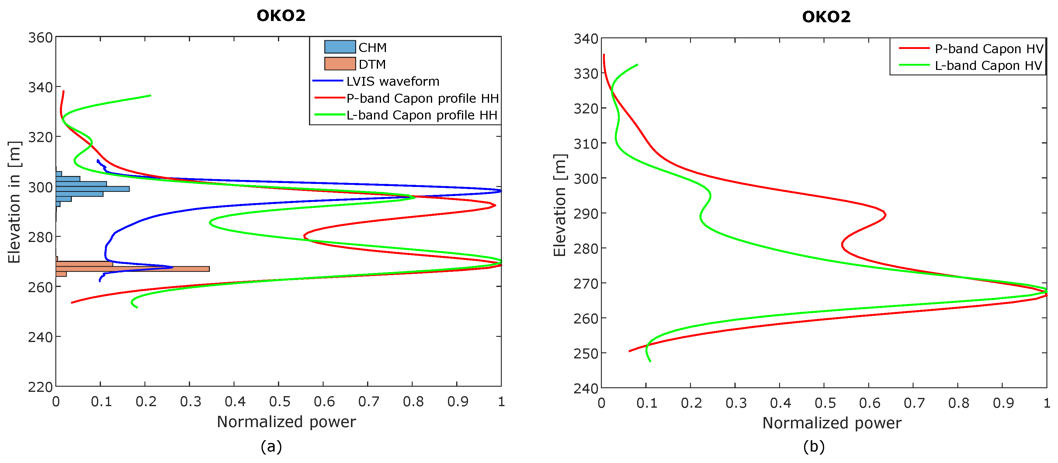
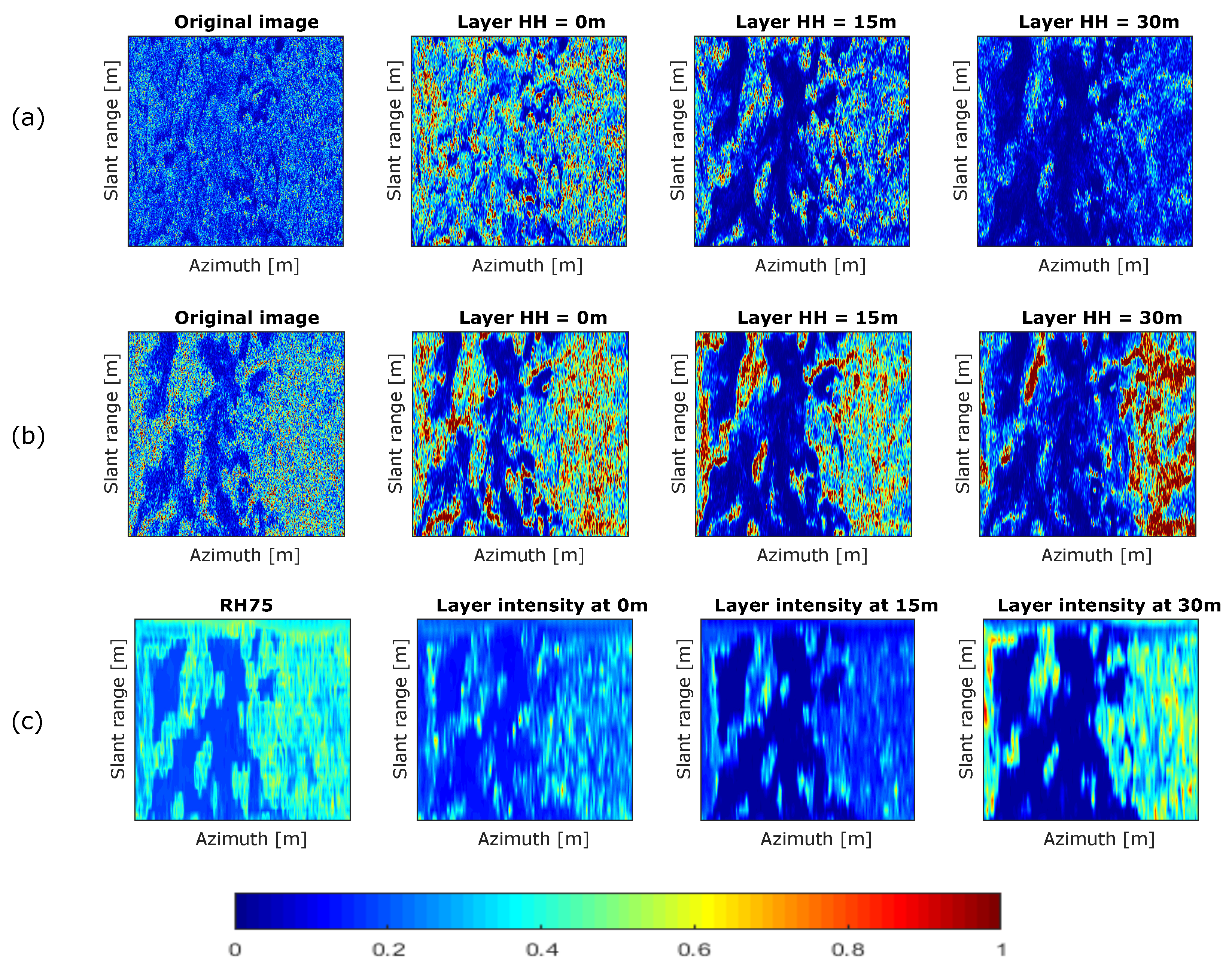
3.3. TomoSAR Multi-Layers

Figure 10 shows the HH backscatter for the original, ground layer (0 m), 15 m layer, and 30 m layer at P- and L-band and LVIS Level 1B data. It is noticed that the ground layer image is characterized by better contrast information compared to the original data at both P- and L-band. This can be explained as the signal at ground level being focused on the tomography processing, and rejecting contributions from the upper vegetation allows a better characterization of the polarimetric signature of ground scattering.

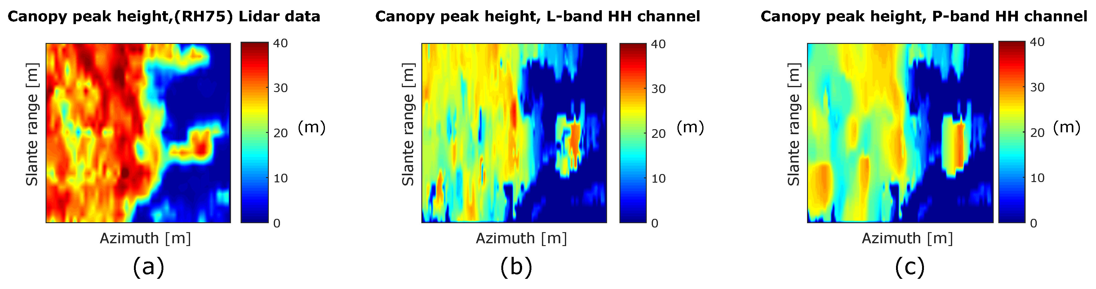
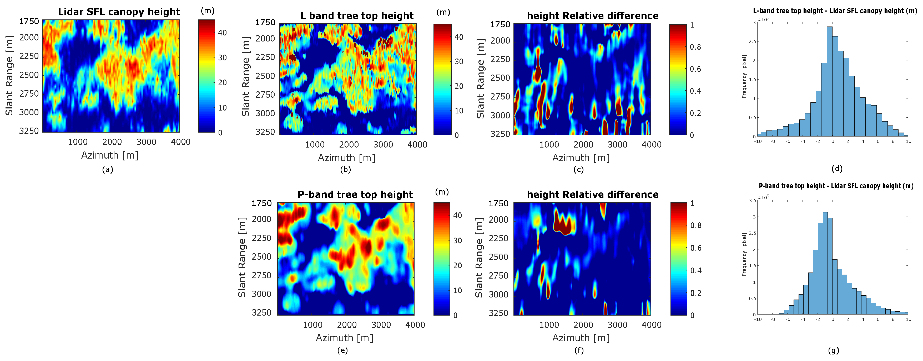
3.4. Forest Top Height Estimation from L- and P-Band

In Figure 11a, the CHM from SFL data is shown, while Figure 11b shows the forest top height estimated from L-band TomoSAR data in the same area. The relative differences between L-band CHM and SFL CHM data are shown in Figure 9c (Relative height difference = (LbandCHM − (LidarCHM)/(LidarCHM)). Figure 11e presents the forest top height estimated from P-band data. The relative difference between P-band CHM and SFL CHM data are shown in Figure 11f (Relative height difference = (PbandCHM − (LiDARCHM)/(LiDARCHM)). The difference between the estimated height from L-band, P-band and CHM from SFL data are shown in Figure 11d,g, respectively. The bias of the difference (histogram) between L-band CHM and SFL CHM is equal to −0.0681, where the RMSE value is 3.68 m; the coefficient of determination shows a value of 0.93. Regarding the histogram of the difference between P-band CHM and SFL CHM, the bias value is equal to −0.1151, where the RMSE value is equal to 3.02 m, and the coefficient of determination shows a value of 0.95.

4. Discussion

In this work, the ability of L-band TomoSAR imaging to retrieve tropical forest structure parameters has been assessed. A tomographic study was implemented using L-band NASA/JPL UAVSAR data, and P-band SETHI data from ONERA collected during the AfriSAR campaign in 2015 and 2016. We show L- and P-band tomograms at different sections of the Lopé and we validated it with CHM from SFL data. We demonstrated that the analysis is improved significantly when the airborne data were corrected for the residual phases related to the perturbations because of motions and flight trajectories uncertainties during the data acquisitions. The impact of phase screen correction in the tomographic inversion is displayed, where it is shown in the tomogram at slant range cut before and after phase calibration. A qualitative comparison is made between Capon profiles from L- and P-band data and LVIS waveforms at a region of interest named OKO2 in the Gabon Lopé Park. Finally, the forest top height from UAVSAR and SETHI data has been estimated. Together, these results confirm our expectation in the ability of TomoSAR to characterize the tropical forests 3D structure accurately.

4.1. Limitation of L-Band TomoSAR in Tropical Forest (TropiSAR Data)

The average Height of Ambiguity in L-band tomographic TropiSAR data are about 30 m in the near range and 50 m in the far range. The L-band tomogram is quite disturbed when compared to the P-band tomogram (Figure 4) for a dense forest of 30 m and above. In this condition, the use of tomographic imaging at L-band in tropical forests appears limited. Such limitation needs more elaborated processing either in the configuration setup of the acquisitions or in the tomographic techniques and phase calibration. However, when the forest top height is roughly below 20 m (e.g., in forest regrowth), the tomographic results are expected to be the same as in boreal forests.

4.2. TomoSAR Profiles at L- and P-Band (AfriSAR Data)

The analysis is done here in the azimuth direction for a fixed slant range positions (sliding window centered on the pixel number 300 m and 650 m). The Capon profile for the HH channel is shown in Figure 6 for the corrected data only. In this profile, it can be noticed that, even if the SFL data and the corrected tomographic profiles seem to show generally a good correlation at the two bands L and P, the mean SFL elevations can sometimes be notably different from the positions of the peaks of the Capon profiles. This could be linked to the SFL data that do not describe the same location due to the difference in penetration capabilities between radar signals and SFL or to other uncompensated effects. After analyzing the histograms of Figure 8, the differences in the canopy height peak estimated from L-band, P-band, and LiDAR waveform are mainly originated from the difference in the penetration capabilities of TomoSAR at L- and P-band, and the LiDAR LVIS platform. In addition, this was expected. The platform resolution is another cause for the high observed bias.
The same interpretation is carried out for a specific region of interest in the Lopé named OKO2. The difference in the vegetation profile shapes between the LVIS and the Capon profiles may be originated from a difference in penetration capabilities or a variation of profile resolution between LVIS and TomoSAR data. After comparing the LVIS and the Capon profiles, the results show significant similarities. Despite the fact that tomography SAR in L & P bands with Capon estimator may not be able to produce vertical profiles with a resolution as good as the LVIS imaging system, it can always reveal stronger ground contribution as shown in the studied ROI (OKO2).

4.3. TomoSAR Multi-Layers

By observing Figure 10, and by comparing with the original SAR image at L- and P-band TomoSAR data, we found that the ground layer image has better contrast information. This implies that a ground-level signal is focused by tomography processing, thus rejecting contributions from vegetation layers and permitting the characterization of polarimetric signature of the ground scattering. The behavior of a polarimetric signature can be studied with respect to the topographic terrain ground slope. It often uses a physical model for interpreting this behavior to better understand the various scattering mechanisms (single bounce, double bounce). To compare with TomoSAR layers, the LVIS Level 1B and level 2 data as tomography were processed through reconstructing the LiDAR waveform along the z-axis; thus, the LVIS multi-layer similar to TomoSAR layers was obtained (Figure 10). Qualitatively, regarding the ground layer (or 0 m), no ground contribution is present because of the LiDAR LVIS penetration capabilities, which are lower than those of SAR.

4.4. Forest Top Height Estimation from L- and P-Band

The canopy height estimation is performed using the L-and P-band TomoSAR data in the Gabon Lopé National Park. By evaluating the vertical forests structure from tomographic profiles, the forests’ top height can be retrieved using CHM from SFL data as a reference. Here, RMSE was estimated to be 3.68 m for L-band TomoSAR as Figure 11d, while the value of RMSE is 3.02 m using P-band TomoSAR data. This reveals as before that no limitation is present for the implementation of canopy height retrieval algorithm with the L-band and P-band TomoSAR. The penetration performance of P-band is better than that of L-band due to its longer wavelength. The latter permits fewer interactions with the leaves and the branches, thus leading to deeper penetration of the radar signals to reach the ground layer. In order to give precise knowledge about the accuracy of the proposed method that is applied in estimating the forest top height, Figure 11c,f show the spatial distribution of height differences between L-band TomoSAR, P-band TomoSAR and that of LiDAR height. By analyzing the histogram of Figure 11d,g, one can notice that the height difference histogram between TomoSAR and LiDAR tends to be normally distributed. Our results considerably reinforce the proposal that L-band TomoSAR will be able to provide a highly accurate 3D vertical structure even in the densest forests worldwide.

4.5. Forest Structure Indices and Parameters

As prospective work, we aim to estimate the forest structure indices as the vertical and the horizontal indices that support biomass retrieval algorithms and enhance forest management activities. However, the forest structure is an important factor in its ecology as it is correlated with many ecological processes [40,41,42]. Furthermore, it is also used as an indicator to detect the biodiversity, where the vertically structured forests foster some taxa biodiversity [43,44,45]. In addition, either the horizontal or the vertical structural heterogeneity can enhance the forest ecosystems’ resistance against disturbances [46,47]. Previous studies have also explored the forest structure’s effects on the productivity of the forest [45,48,49,50], where they found that the main drivers of the productivity of forest are the variables that characterize the structure of the forest rather than the biodiversity-related variables. Though it is highly important to know the structure of the forest in order to understand its dynamics, there are still no available global forest structure maps yet. There are only a few coarse-resolution maps that are present, but these only show the components of the structure of forest (e.g., the height of a forest from MODIS and ICESat, resolution 1 km, Indeed, larger regions of multi-layered forest structure should be efficiently analyzed. Recent satellite missions have been (e.g., GEDI, ICEsat2 sensor) and will be launched (e.g., BIOMASS, and Tandem-L) where new technologies will be used in order to measure, on a global scale, the structure of forest including its height and its vertical heterogeneity. Nowadays, there are two main elements: the vertical and horizontal forest structures [11,48,51,52]. Finding a clear and suitable definition for forest structure is highly difficult. Furthermore, the metrics of forest structure differ depending on whether they are based either on remote sensing or on field data. The remote sensing-based descriptors often depend on the heterogeneous canopy structure for a given area; however, the field-based descriptors for the forest structure are derived from size measurements of each individual tree [51]. Terrestrial Laser Scanning (TLS) is a hybrid approach for forest structure, which is measured by both field and remote sensing data [53]. It gives highly detailed measurements for every single tree and for the forest canopy structure. TLS is the best replacement for plot-level inventory data in many systems. We note hereby that TLS cannot be considered as an alternative to large extent remote sensing techniques, but it is a critical component of calibration and validation of EO products. Therefore, in order to capture forest structure on a larger scale, either airborne or satellite-based remote sensing data could be suitable choices for this.
In our future studies, we are interested in using the forest modeling, LiDAR remote sensing, and airborne TomoSAR in order to be able to answer the question, “How can we estimate structure of a forest by using remote sensing, and what is the role played by forest structure in estimating the forest biomass and the above-ground wood productivity?” Our aim is to use the vertical and horizontal descriptors that can be measured by remote sensing in order to classify the forests into structural categories. Using this structural classification, we will explore if we will be able to estimate more accurately both forest biomass and above-ground wood productivity in case we included the structural information.

5. Conclusions

In this work, TomoSAR analysis has been applied for the estimation of the forests’ canopy height and terrain using L-band UAVSAR and P-band SETHI from AfriSAR data, collected over the Gabon Lopé Park on 2015 and 2016. Prior to tomographic imaging, a phase residual correction methodology based on phase calibration via phase center double localization was implemented. The tomographic P- and L-band Capon profiles at different sections in the forests are validated in a good correlation with SFL LiDAR data CHM from the SFL data set as a reference. Second, the vertical profile of the vegetation at different sections in the Lopé using a Capon power estimator at HH, HV polarizations with LVIS Level 1B waveform LiDAR data, carried out over the OKO2 region in the Gabon Lopé National Park, was compared. The 3D profiles from Lidar waveform and from L- and P-band TomoSAR data show a high correlation. Finally, we report on the performance of forests’ top height retrieved from the TomoSAR L-band and P-band data. Forests’ top height from TomoSAR data that are estimated and validated with SFL data have an RMSE of 3.68 m for the L-band data. The RMSE value of P-band forest top height with respect to SFL was 3.02 m. The corresponding coefficient of determination was 0.95 and 0.93 for P- and L-band, respectively. Together, these results demonstrate the potential of TomoSAR to retrieve forest structure parameters. The development of tomographic SAR techniques allows for the reconstruction of the 3D radar reflectivity opening the door for 3D forest monitoring. As the link between physical forest structure and the reconstructed 3D radar reflectivity is still not understood and is far from being established, the 3D radar profiles obtained open prospects to derive algorithms that are able to link these profiles to the physical structure of the forest. For future work, we aim to provide an algorithm to estimate horizontal and vertical structure descriptors. These descriptors can be derived from TomoSAR data, which allow the characterization of the physical forest structure. Horizontal and vertical structure descriptors are crucial in boosting up the performance of biomass estimators. We hope that our results reinforce the scientific basis to estimate tropical forests’ structure indices and give support for the upcoming biomass missions.

Author Contributions

Conceptualization, I.E.M. and D.H.T.M.; Data curation, I.E.M. and Y.N.N.; Methodology, I.E.M.; Project administration, N.B., J.J., O.S. and C.A.; Supervision, D.H.T.M. and C.A.; Validation, I.E.M. and D.H.T.M.; Visualization, I.E.M., D.H.T.M., M.L. and N.B.; Writing—original draft, I.E.M., Writing—review and editing, I.E.M., D.H.T.M., N.B., C.A., J.J., O.S., M.L. and Y.N.N.

Funding

Financial support from the “UM-AUF-CNRSL grant” (University of Montpellier, L’Agence Universitaire de la Francophonie (AUF), and the National Council for Scientific Research in Lebanon (CNRSL) are greatly appreciated for I.E.M’s grants. IRSTEA (National Research Institute of Science and Technology for Environment and Agriculture) also acknowledged.

Acknowledgments

The authors would like to acknowledge the National Aeronautics and Space Administration (NASA) for providing the UAVSAR data, LVIS LiDAR data, and Small FootPrint LiDAR SFL data. In addition, the authors would like to acknowledge Office National 125 d’tudes Et de Recherches Arospatiales (ONERA) for providing P-band SETHI tomography data. The ESA and the BIOSAR team are gratefully acknowledged for funding and collecting the tomography data at Krycklan, Sweden.

Conflicts of Interest

The authors declare no conflict of interest.

References

  1. Wright, S.J. Tropical forests in a changing environment. Trends Ecol. Evol. 2005, 20, 553–560. [Google Scholar] [CrossRef] [PubMed]
  2. Spies, T.A. Forest structure: A key to the ecosystem. Northwest Sci. 1998, 72, 34–36. [Google Scholar]
  3. Grace, J. Understanding and managing the global carbon cycle. J. Ecol. 2004, 92, 189–202. [Google Scholar] [CrossRef]
  4. Gatti, L.; Gloor, M.; Miller, J.; Doughty, C.; Malhi, Y.; Domingues, L.; Basso, L.; Martinewski, A.; Correia, C.; Borges, V.; et al. Drought sensitivity of Amazonian carbon balance revealed by atmospheric measurements. Nature 2014, 506, 76–80. [Google Scholar] [CrossRef] [PubMed]
  5. Frolking, S.; Palace, M.W.; Clark, D.; Chambers, J.Q.; Shugart, H.; Hurtt, G.C. Forest disturbance and recovery: A general review in the context of spaceborne remote sensing of impacts on aboveground biomass and canopy structure. J. Geophys. Res. Biogeosci. 2009, 114. [Google Scholar] [CrossRef]
  6. Fischer, R.; Knapp, N.; Bohn, F.; Shugart, H.H.; Huth, A. The relevance of forest structure for biomass and productivity in temperate forests: New perspectives for remote sensing. Surv. Geophys. 2019, 40, 709–734. [Google Scholar] [CrossRef]
  7. Hall, F.G.; Bergen, K.; Blair, J.B.; Dubayah, R.; Houghton, R.; Hurtt, G.; Kellndorfer, J.; Lefsky, M.; Ranson, J.; Saatchi, S.; et al. Characterizing 3D vegetation structure from space: Mission requirements. Remote Sens. Environ. 2011, 115, 2753–2775. [Google Scholar] [CrossRef] [Green Version]
  8. Bergen, K.; Goetz, S.; Dubayah, R.; Henebry, G.; Hunsaker, C.; Imhoff, M.; Nelson, R.; Parker, G.; Radeloff, V. Remote sensing of vegetation 3D structure for biodiversity and habitat: Review and implications for lidar and radar spaceborne missions. J. Geophys. Res. Biogeosci. 2009, 114. [Google Scholar] [CrossRef]
  9. Goetz, S.; Steinberg, D.; Dubayah, R.; Blair, B. Laser remote sensing of canopy habitat heterogeneity as a predictor of bird species richness in an eastern temperate forest, USA. Remote Sens. Environ. 2007, 108, 254–263. [Google Scholar] [CrossRef]
  10. Turner, W.; Spector, S.; Gardiner, N.; Fladeland, M.; Sterling, E.; Steininger, M. Remote sensing for biodiversity science and conservation. Trends Ecol. Evol. 2003, 18, 306–314. [Google Scholar] [CrossRef]
  11. Tello, M.; Cazcarra-Bes, V.; Pardini, M.; Papathanassiou, K. Forest Structure Characterization From SAR Tomography at L-Band. IEEE J. Sel. Top. Appl. Earth Obs. Remote Sens. 2018, 11, 3402–3414. [Google Scholar] [CrossRef] [Green Version]
  12. Beaudoin, A.; Le Toan, T.; Goze, S.; Nezry, E.; Lopes, A.; Mougin, E.; Hsu, C.; Han, H.; Kong, J.; Shin, R. Retrieval of forest biomass from SAR data. Int. J. Remote Sens. 1994, 15, 2777–2796. [Google Scholar] [CrossRef]
  13. Treuhaft, R.N.; Siqueira, P.R. Vertical structure of vegetated land surfaces from interferometric and polarimetric radar. Radio Sci. 2000, 35, 141–177. [Google Scholar] [CrossRef] [Green Version]
  14. Garestier, F.; Dubois-Fernandez, P.C.; Guyon, D.; Le Toan, T. Forest biophysical parameter estimation using L-and P-band polarimetric SAR data. IEEE Trans. Geosci. Remote Sens. 2009, 47, 3379–3388. [Google Scholar] [CrossRef]
  15. Cloude, S.R.; Papathanassiou, K.P. Polarimetric SAR interferometry. IEEE Trans. Geosci. Remote Sens. 1998, 36, 1551–1565. [Google Scholar] [CrossRef]
  16. Cloude, S.; Papathanassiou, K. Three-stage inversion process for polarimetric SAR interferometry. IEE Proc. Radar Sonar Navig. 2003, 150, 125–134. [Google Scholar] [CrossRef] [Green Version]
  17. Reigber, A.; Moreira, A. First, demonstration of airborne SAR tomography using multibaseline L-band data. IEEE Trans. Geosci. Remote Sens. 2000, 38, 2142–2152. [Google Scholar] [CrossRef]
  18. Frey, O.; Meier, E. Analyzing tomographic SAR data of a forest with respect to frequency, polarization, and focusing technique. IEEE Trans. Geosci. Remote Sens. 2011, 49, 3648–3659. [Google Scholar] [CrossRef]
  19. Neumann, M.; Ferro-Famil, L.; Reigber, A. Estimation of forest structure, ground, and canopy layer characteristics from multibaseline polarimetric interferometric SAR data. IEEE Trans. Geosci. Remote Sens. 2010, 48, 1086–1104. [Google Scholar] [CrossRef]
  20. Caicoya, A.T.; Pardini, M.; Hajnsek, I.; Papathanassiou, K. Forest above-ground biomass estimation from vertical reflectivity profiles at L-band. IEEE Geosci. Remote Sens. Lett. 2015, 12, 2379–2383. [Google Scholar] [CrossRef]
  21. Tebaldini, S.; Rocca, F. Multibaseline polarimetric SAR tomography of a boreal forest at P-and L-bands. IEEE Trans. Geosci. Remote Sens. 2012, 50, 232–246. [Google Scholar] [CrossRef]
  22. Aguilera, E.; Nannini, M.; Reigber, A. Wavelet-based compressed sensing for SAR tomography of forested areas. IEEE Trans. Geosci. Remote Sens. 2013, 51, 5283–5295. [Google Scholar] [CrossRef]
  23. Pardini, M.; Papathanassiou, K. Sub-canopy topography estimation: Experiments with multibaseline SAR data at L-band. In Proceedings of the 2012 IEEE International Geoscience and Remote Sensing Symposium, Munich, Germany, 22–27 July 2012; pp. 4954–4957. [Google Scholar]
  24. Le Toan, T.; Quegan, S.; Davidson, M.; Balzter, H.; Paillou, P.; Papathanassiou, K.; Plummer, S.; Rocca, F.; Saatchi, S.; Shugart, H.; et al. The BIOMASS mission: Mapping global forest biomass to better understand the terrestrial carbon cycle. Remote Sens. Environ. 2011, 115, 2850–2860. [Google Scholar] [CrossRef] [Green Version]
  25. Krieger, G.; Moreira, A.; Zink, M.; Hajnsek, I.; Huber, S.; Villano, M.; Papathanassiou, K.; Younis, M.; Dekker, P.L.; Pardini, M.; et al. Tandem-L: Main results of the phase a feasibility study. In Proceedings of the 2016 IEEE International Geoscience and Remote Sensing Symposium (IGARSS), Beijing, China, 10–15 July 2016; pp. 2116–2119. [Google Scholar]
  26. Gini, F.; Lombardini, F.; Montanari, M. Layover solution in multibaseline SAR interferometry. IEEE Trans. Aerosp. Electron. Syst. 2002, 38, 1344–1356. [Google Scholar] [CrossRef]
  27. Tebaldini, S. Algebraic synthesis of forest scenarios from multibaseline PolInSAR data. IEEE Trans. Geosci. Remote Sens. 2009, 47, 4132–4142. [Google Scholar] [CrossRef]
  28. Huang, Y.; Ferro-Famil, L.; Reigber, A. Under-foliage object imaging using SAR tomography and polarimetric spectral estimators. IEEE Trans. Geosci. Remote Sens. 2012, 50, 2213–2225. [Google Scholar] [CrossRef]
  29. Minh, D.H.T.; Le Toan, T.; Rocca, F.; Tebaldini, S.; Villard, L.; Réjou-Méchain, M.; Phillips, O.L.; Feldpausch, T.R.; Dubois-Fernandez, P.; Scipal, K.; et al. SAR tomography for the retrieval of forest biomass and height: Cross-validation at two tropical forest sites in French Guiana. Remote Sens. Environ. 2016, 175, 138–147. [Google Scholar] [CrossRef] [Green Version]
  30. Minh, D.H.T.; Le Toan, T.; Rocca, F.; Tebaldini, S.; d’Alessandro, M.M.; Villard, L. Relating P-band synthetic aperture radar tomography to tropical forest biomass. IEEE Trans. Geosci. Remote Sens. 2014, 52, 967–979. [Google Scholar] [CrossRef]
  31. Sauer, S.; Ferro-Famil, L.; Reigber, A.; Pottier, E. Multibaseline POL-InSAR analysis of urban scenes for 3D modeling and physical feature retrieval at L-band. In Proceedings of the 2007 IEEE International Geoscience and Remote Sensing Symposium, Barcelona, Spain, 23–28 July 2007; pp. 1098–1101. [Google Scholar]
  32. Fornaro, G.; Lombardini, F.; Serafino, F. Three-dimensional multipass SAR focusing: Experiments with long-term spaceborne data. IEEE Trans. Geosci. Remote Sens. 2005, 43, 702–714. [Google Scholar] [CrossRef]
  33. Cloude, S.R. Dual-baseline coherence tomography. IEEE Geosci. Remote Sens. Lett. 2007, 4, 127–131. [Google Scholar] [CrossRef]
  34. Cloude, S.R. Multifrequency 3D imaging of tropical forest using polarization coherence tomography. In Proceedings of the 7th European Conference on Synthetic Aperture Radar, Friedrichshafen, Germany, 2–5 June 2008; pp. 1–4. [Google Scholar]
  35. Minh, D.H.T.; Le Toan, T.; Tebaldini, S.; Rocca, F.; Iannini, L. Assessment of the P-and L-band SAR tomography for the characterization of tropical forests. In Proceedings of the 2015 IEEE International Geoscience and Remote Sensing Symposium (IGARSS), Milan, Italy, 26–31 July 2015; pp. 2931–2934. [Google Scholar]
  36. Lee, J. Forest-savanna dynamics and the origins of Marantaceae forest in central Gabon. In African Rain Forest Ecology and Conservation: An Interdisciplinary Perspective; Yale University Press: New Haven, CT, USA, 2001; p. 165. [Google Scholar]
  37. Tebaldini, S.; Rocca, F.; d’Alessandro, M.M.; Ferro-Famil, L. Phase calibration of airborne tomographic sar data via phase center double localization. IEEE Trans. Geosci. Remote Sens. 2015, 54, 1775–1792. [Google Scholar] [CrossRef]
  38. Stoica, P.; Moses, R.L. Spectral Analysis of Signals; Prentice Hall, Inc.: Upper Saddle River, NJ, USA, 2005. [Google Scholar]
  39. El Moussawi, I.; Ho Tong Minh, D.; Baghdadi, N.; Abdallah, C.; Jomaah, J.; Strauss, O.; Lavalle, M. L-Band UAVSAR Tomographic Imaging in Dense Forests: Gabon Forests. Remote Sens. 2019, 11, 475. [Google Scholar] [CrossRef]
  40. Pretzsch, H.; Dieler, J.; Matyssek, R.; Wipfler, P. Tree and stand growth of mature Norway spruce and European beech under long-term ozone fumigation. Environ. Pollut. 2010, 158, 1061–1070. [Google Scholar] [CrossRef]
  41. Shugart, H.; Saatchi, S.; Hall, F. Importance of structure and its measurement in quantifying function of forest ecosystems. J. Geophys. Res. Biogeosci. 2010, 115. [Google Scholar] [CrossRef]
  42. Mundell, J.; Taff, S.J.; Kilgore, M.; Snyder, S. Using real estate records to assess forest land parcelization and development: A Minnesota case study. Landsc. Urban Plan. 2010, 94, 71–76. [Google Scholar] [CrossRef]
  43. Boncina, A. Comparison of structure and biodiversity in the Rajhenav virgin forest remnant and managed forest in the Dinaric region of Slovenia. Glob. Ecol. Biogeogr. 2000, 9, 201–211. [Google Scholar] [CrossRef]
  44. Ishii, H.T.; Tanabe, S.I.; Hiura, T. Exploring the relationships among canopy structure, stand productivity, and biodiversity of temperate forest ecosystems. For. Sci. 2004, 50, 342–355. [Google Scholar]
  45. Schall, P.; Gossner, M.M.; Heinrichs, S.; Fischer, M.; Boch, S.; Prati, D.; Jung, K.; Baumgartner, V.; Blaser, S.; Böhm, S.; et al. The impact of even-aged and uneven-aged forest management on regional biodiversity of multiple taxa in European beech forests. J. Appl. Ecol. 2018, 55, 267–278. [Google Scholar] [CrossRef]
  46. Dobbertin, M. Tree growth as indicator of tree vitality and of tree reaction to environmental stress: A review. Eur. J. For. Res. 2005, 124, 319–333. [Google Scholar] [CrossRef]
  47. Pretzsch, H.; Del Río, M.; Schütze, G.; Ammer, C.; Annighöfer, P.; Avdagic, A.; Barbeito, I.; Bielak, K.; Brazaitis, G.; Coll, L.; et al. Mixing of Scots pine (Pinus sylvestris L.) and European beech (Fagus sylvatica L.) enhances structural heterogeneity, and the effect increases with water availability. For. Ecol. Manag. 2016, 373, 149–166. [Google Scholar] [CrossRef]
  48. Bohn, F.J.; Huth, A. The importance of forest structure to biodiversity–productivity relationships. R. Soc. Open Sci. 2017, 4, 160521. [Google Scholar] [CrossRef]
  49. Dănescu, A.; Albrecht, A.T.; Bauhus, J. Structural diversity promotes productivity of mixed, uneven-aged forests in southwestern Germany. Oecologia 2016, 182, 319–333. [Google Scholar] [CrossRef]
  50. Liu, Y.Y.; Wang, Y.; Walsh, T.R.; Yi, L.X.; Zhang, R.; Spencer, J.; Doi, Y.; Tian, G.; Dong, B.; Huang, X.; et al. Emergence of plasmid-mediated colistin resistance mechanism MCR-1 in animals and human beings in China: A microbiological and molecular biological study. Lancet Infect. Dis. 2016, 16, 161–168. [Google Scholar] [CrossRef]
  51. Cazcarra-Bes, V.; Tello-Alonso, M.; Fischer, R.; Heym, M.; Papathanassiou, K. Monitoring of forest structure dynamics by means of L-band SAR tomography. Remote Sens. 2017, 9, 1229. [Google Scholar] [CrossRef]
  52. Getzin, S.; Wiegand, K.; Schöning, I. Assessing biodiversity in forests using very high-resolution images and unmanned aerial vehicles. Methods Ecol. Evol. 2012, 3, 397–404. [Google Scholar] [CrossRef]
  53. Stovall, A.E.; Shugart, H.H. Improved biomass calibration and validation with terrestrial LiDAR: Implications for future LiDAR and SAR missions. IEEE J. Sel. Top. Appl. Earth Obs. Remote Sens. 2018, 11, 3527–3537. [Google Scholar] [CrossRef]
Figure 1. TropiSAR, BioSAR, and AfriSAR Campaigns. Study area main site (Gabon Lopé National park). The red polygon denotes the footprint of L-band UAVSAR platform. The Digital elevation model of the Lopé is displayed.
Remotesensing 11 01934 g001
Figure 2. TomoSAR acquisition.
Remotesensing 11 01934 g002
Figure 3. Phase calibration problem formulation.
Remotesensing 11 01934 g003
Figure 4. (a) L-band Tomogram (HH channel) at Tropical Paracou forest; (b) P-band Tomogram (HH channel) at Tropical Paracou forest; (c) L-band Tomogram (HH channel) at Boreal Krycklan forest; (d) P-band Tomogram (HH channel) at Boreal Krycklan forest. The algorithm used to get the tomography profiles is the Capon beamforming power estimator.
Remotesensing 11 01934 g004
Figure 5. (a) 2D intensity of SLC P-band image. The red line denotes the cut where the Capon beamforming estimator was applied; (b) P-band Tomogram (HH channel) before applying phase screen correction; (c) P-band Tomogram (HH channel) after applying phase screen correction.
Remotesensing 11 01934 g005
Figure 6. (a) and (f) SFL CHM LiDAR cuts at slant range equal to 300 m and 650 m; (b) and (g) 2D intensity L-band SLC image. The red line denotes the cut where we had chosen to estimate the vertical structure along with slant range; (c) and (h) L-band HH channel Tomographic profile at the two cuts (300 m and 650 m); (d) and (i) P-band HH channel Tomographic profile at the two cuts (300 m and 650 m); (e) and (j) LVIS data layers from LiDAR LVIS Level 1B at the two cut, defined befors (300 m and 650 m). The white line in all tomograms denote the RH75 height from LiDAR LVIS Level2 data.
Remotesensing 11 01934 g006
Figure 7. (a) canopy peak height estimated from LiDAR waveform (RH75); (b) canopy peak height estimated from L-band data; (c) canopy peak height estimated from P-band data.
Remotesensing 11 01934 g007
Figure 8. (a) histogram of the difference between canopy peak height estimated from P-band data and canopy peak height estimated from L-band data; (b) histogram of the difference between canopy peak height estimated from L-band data and canopy peak height estimated from LiDAR LVIS Level1B data (or RH75 from LiDAR LVIS Level2 data); (c) histogram of the difference between canopy peak height estimated from P-band data and canopy peak height estimated from LiDAR LVIS Level1B data.
Remotesensing 11 01934 g008
Figure 9. (a) region of interest (ROI) named OKO2 in Gabon Lopé Park. P-band HH (in red) and L-band HH (in green) Capon profiles. Capon power and LVIS waveform power were normalized between 0 and 1. The histograms of SFL canopy and ground elevations are presented respectively in blue and brown. The blue curve corresponds to LVIS waveform Level 1B; (b) P-band Capon HV profile in red. L-band Capon HV profile in green.
Remotesensing 11 01934 g009
Figure 10. (a) original SAR image. HH power intensities associated with an L-band SAR with three layers produced by TomoSAR: 0 m, 15 m, 30 m; (b) original SAR image. HH power intensities associated with a P-band SAR with three layers produced by TomoSAR: 0 m, 15 m, 30 m; (c) power intensities associated with LVIS data layers produced from LiDAR LVIS Level 1B data: 0 m, 15 m, 30 m.
Remotesensing 11 01934 g010
Figure 11. (a) CHM from SFL data; (b) forest top height estimated from L-band TomoSAR data; (c) relative difference between LiDAR and L-band TomoSAR tree top height, height difference = (HTomo − HLiDAR)./HLiDAR; (d) histogram of the difference between the estimated height from L-band and CHM from SFL data; (e) forest top height estimated from P-band TomoSAR data; (f) relative difference between LiDAR and P-band TomoSAR tree top height, height difference = (HTomo − HLiDAR)./HLiDAR; (g) histogram of the difference between the estimated height from P-band and CHM from SFL data.
Remotesensing 11 01934 g011
Table 1. L-band UAVSAR acquisition parameters.
Acquisition Parameters
Acquisition ModePolSAR
Look DirectionLeft looking
Pulse duaration40 ( μ s)
Steering Angle90 (deg)
Bandwidth80 (MHz)
Ping-Pong or Single Antenna TransmitPing-Pong
Air craft speed224 (m/s)
Range of look angle21–65 (deg)
Antenna Length1.5 (m)
Table 2. Description of the SETHI system configuration of P-band acquisition parameters. The superscript * indicates the parameters that are identical between the SETHI and F-SAR systems.
Acquisition Parameters
Acquisition Mode *PolSAR
Look DirectionLeft looking
Effective Pulse Repition Frequency (PRF)1250 (Hz)
Steering Angle90 (deg)
Frequency range */Bandwidth50 (MHz)
Pulse duration30 ( μ s)
Transmitted power500 (W)
Aircraft speed100–150 (m/s)
Flight ground altitude6096 (m)

