Quantification of Hydrocarbon Abundance in Soils Using Deep Learning with Dropout and Hyperspectral Data

Abstract

Terrestrial hydrocarbon spills have the potential to cause significant soil degradation across large areas. Identification and remedial measures taken at an early stage are therefore important. Reflectance spectroscopy is a rapid remote sensing method that has proven capable of characterizing hydrocarbon-contaminated soils. In this paper, we develop a deep learning approach to estimate the amount of Hydrocarbon (HC) mixed with different soil samples using a three-term backpropagation algorithm with dropout. The dropout was used to avoid overfitting and reduce computational complexity. A Hyspex SWIR 384 m camera measured the reflectance of the samples obtained by mixing and homogenizing four different soil types with four different HC substances, respectively. The datasets were fed into the proposed deep learning neural network to quantify the amount of HCs in each dataset. Individual validation of all the dataset shows excellent prediction estimation of the HC content with an average mean square error of ~2.2 × 10⁻⁴. The results with remote sensed data captured by an airborne system validate the approach. This demonstrates that a deep learning approach coupled with hyperspectral imaging techniques can be used for rapid identification and estimation of HCs in soils, which could be useful in estimating the quantity of HC spills at an early stage.

1. Introduction

Hydrocarbons refer to chemical substances formed exclusively from carbon and hydrogen. Naturally occurring hydrocarbon (HC) substances, depending on the length of the carbon chain, occur in different forms; solid, liquid, and gas [1]. Liquid HCs found in nature consist of a complex mixture of various molecular weights; in addition nitrogen, sulfur, and oxygen exist in small quantities [2].

While the economic significance of HCs is attributed to its primary use as fuel and then versatile application in downstream industries, they can have detrimental environmental consequences [1,3]. Oil exploration, production, and processing represent potential environmental exposure to HCs resulting in accidental terrestrial spillage thereby altering the physical and chemical properties of soils. HCs may therefore be environmentally harmful, causing toxicity, and limiting soil quality [4].

Knowledge about the concentration and nature of a spill is important in order to track their propagation in the environment, assess their risk and propose remediation strategies [5,6]. To effectively protect communities affected by a spill, fast and accurate determination of the area impacted is needed, particularly if monitoring large regions affected by an oil spill or where aged oil transporting facilities are involved [7]. Traditional methods employed to track and detect oil spills and the concentration of HCs in soils often involve processes which are expensive and time consuming as they require field sampling, chemical analysis, and geostatistical interpolation [8,9]. Imaging spectroscopy has been recognized as a reliable alternative method for detecting HCs in soils and is rapid and cost-effective [6,10].

Imaging spectroscopy (hyperspectral imaging) can be described as the combination of digital imaging and spectroscopy. A hyperspectral camera captures the light intensity for a large number of spectral bands, providing much more information about a scene when compared to a standard camera which only covers the visible wide bandwidth portion of the electromagnetic spectrum [6]. Due to the rich information content in hyperspectral imagery, it is well suited to a range of applications such as crop/vegetation classification, disaster monitoring, oil spill detection, etc. There are several uses of imaging spectroscopy for oil spills, such as the enforcement of ship discharge laws, surveillance and general slick detection, mapping of spills, and direction of spills [11], due to its high spectral and spatial capabilities [12].

More specifically, Near- and Shortwave Infrared (NIR-SWIR) spectroscopes have been popular methods for detecting, mapping, quantifying, and characterizing HCs in contaminated soils with reasonable accuracy [6,13,14]. Moreover, NIR-SWIR spectra provide good information on soils organic and inorganic material content [13]. HCs demonstrate good absorption in spectral bands 1200 nm, 1725 nm, and 2310 nm [5,8,15]. Therefore, spectral information obtained in the NIR-SWIR range is excellent for both the quantitative and qualitative analysis of HCs in soils [13]. Recent works have also successfully demonstrated the use of Longwave Infrared (LWIR) for Petroleum HC detection [16].

Different methods have been used to analyze reflectance spectroscopy data to detect HCs in soils; the authors of [5] used regression analysis and spectral preprocessing to generate statistical models to identify different HC products mixed with a mineral substrate. The authors of [15] used Diffuse Reflectance Infrared Fourier-Transform (DRIFT) spectroscopy which is a hand held spectrometer for the prediction of total petroleum hydrocarbons in contaminated soils. It uses Partial Least Square (PLS) regression analysis, which is a multivariate method and includes correlation between spectral information and corresponding analytical data to rapidly predict the concentration of HCs in soil. Other researchers show the robustness of visible and infrared spectroscopy for the rapid estimation of HCs [17,18].

However, state-of-the art methods for estimating HC concentration in soils mainly concentrate on the quantification of large spills [19]. For instance, the authors of [6] report the estimation of $30\%$ of HC contamination in soils. Recently, the authors of [20] presented regression models based on HC absorption bands in order to estimate the pollution level of different HC. They were able to observe changes in the spectral response, in some cases, for 2% of contaminant and successfully applied their models to identify soils contaminated with just 3% of heavy oil and 14% of diesel. However, the spectrum of soils contaminated with gasoline showed only subtle changes for pollution levels higher than 8%. Thus, they concluded that it would be difficult to detect soils contaminated with gasoline by assessing the VNIR–SWIR interval.

One of the characteristics of hyperspectral remotely sensed data is that the recorded reflectance is the result of multiple interactions of the electromagnetic radiation with the constituents of the soil creating mixed pixels. Numerous studies address the mixing problem and propose analysis techniques [19]. Spectral Unmixing (SU) is the process of identifying spectral signatures of materials, often referred to as endmembers, and then estimate their relative abundance to the measured spectra within a pixel [21]. Endmembers play an important role in exploring spectral information of a hyperspectral image [22,23], as usually the extraction of endmembers, which is the process of obtaining pure signatures of different features present in an image, is the first step in the unmixing algorithms [24,25,26]. SU often requires the definition of the mixing model underlying the observations as presented on the data. A mixing model describes how the endmembers combine to form the mixed spectrum as measured by the sensor [27]. Given the mixing model, SU then estimates the inverse of the formation process to infer the quantity of interest, specifically the endmembers, and abundance from the collected spectra [28,29,30]. This could be achieved through a radiative transfer model that accurately describes light-scattering by the materials in the observed scene by a sensor [27,31]. The two main approaches to spectral unmixing are linear and nonlinear models [21,22,25,26,28].

Different methods utilizing both linear and nonlinear models have been demonstrated in the literature for the analysis of different hydrocarbon types. In a work by the authors of [13,15], Principal Component Analysis (PCA) and PLS regression are used. The authors used PCA to differentiate the types and density of HCs in soils while they used PLS to predict the concentration of oils and fuels in soil samples. The authors of [18] used Spectral Angular Mapper (SAM) to classify oil spills on an image and also used signature matching to distinguish oils from other features. However, most of these methods adopt a linear model and smoothing threshold function for feature extraction. Other approaches such as a Kernel-based transformation [32] and manifold learning algorithm [33] are based on nonlinear models.

In the work by the authors of [34], we proved experimentally that HCs abundance in soils was estimated with higher accuracy when non linear unmixing models were applied. Nevertheless, spectral unmixing and specifically the abundance estimation of HCs such as gasoline, can be challenging [20], and may require more advanced techniques such as deep learning. Deep learning network can be considered a powerful technique to solve nonlinear problems, which can be fast, accurate and does not rely on any assumptions to estimate the abundances in a given dataset. However, to the best of our knowledge, there is no study that uses spectral data and deep learning methods to detect and estimate the percentage of HCs in soils. While the value and application of these two techniques have been presented in independent research activities, the techniques have not yet been combined. Therefore, in this paper, a deep learning approach is developed to estimate the amount of HC contamination in soil samples using SWIR imaging spectroscopy. The remainder of the paper is organized as follows. Section 2 describes the data acquisition process including the materials used, sample preparation and the hyperspectral sensor used. Section 3 discusses the methodology, including the parameters used in training the network, the architecture of the deep learning approach, as well as the validation method. Results are presented in Section 4 and discussed in Section 5. Finally, conclusions are drawn in Section 6.

2. Data Acquisition

2.1. Materials

The hyperspectral imaging sensor used for this experiment covers the Shortwave Infrared (SWIR) range (930–2500 nm), which has been found suitable for the detection of HCs [5,6,13,35,36], mineral identification and mapping [36], rock mapping [37], and mapping of mafic and ultramafic units in the Cape Smith Belt [38].

The soils and HC types selected here have been used extensively in the literature for assessments of HC contamination in different soil types [8,13,17,18,39]. Different HC types, namely Diesel, Bio-diesel, Ethanol, and Petroleum were used. These are the most commonly used HCs in the literature. Soil types include typical mixtures of clay (<$0.002$ mm in diameter), silt (0.002–0.05 mm in diameter), and sand (0.05–1 mm in diameter). In particular, we used mixtures with different grain size ranging from medium to coarse as follows; Clay, Clay Loam , Sand Clay Loam, and Sand Loam [40].

2.2. Sample Preparation

The preparation of the samples consisted of the following steps.

• Each soil type was air-dried, and therefore all samples contained similar levels of moisture.
• Fifty grams of a soil sample type was added to a petri dish (12 cm in diameter)
• The sample was scanned with a Hyspex SWIR 384 m camera under constant illumination.
• In the same sample, initially, 2 mL of the HC were added to the soil using a syringe (to clay and clayloam), which was subsequently changed to 5 mL of the HC to the other soil types.
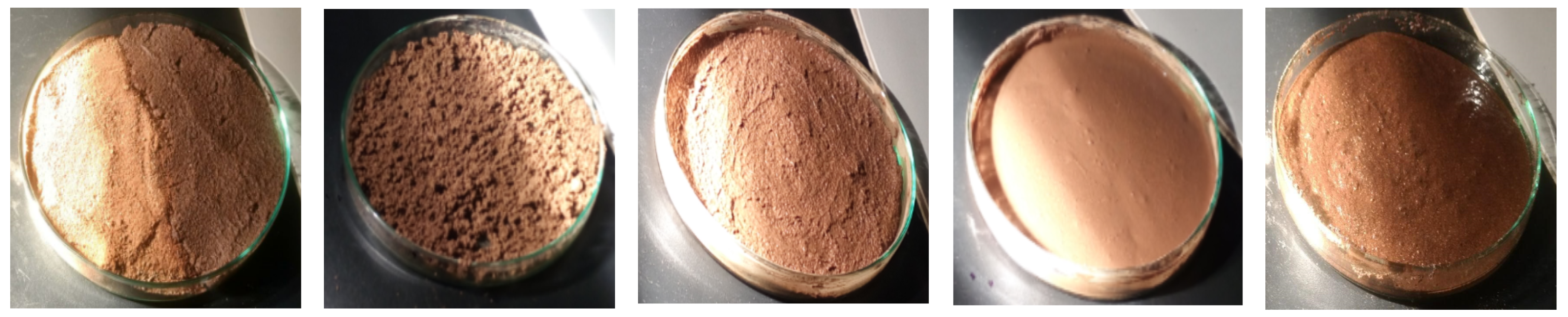
• A disposable plastic spoon was used to homogenize the mixture and to flatten its surface in order to have even surfaces, except for some soil samples containing clay which tends to be sticky and difficult to flatten due to the characteristics of the soil type, e.g., Figure 1b.
• The sample was scanned with a Hyspex SWIR 384 m camera under constant illumination.
• In the same sample, a further 5 mL of HC was added to the mixture.
• The disposable spoon was used to homogenize the mixture and another scan was taken.
• The procedure was repeated with increments of 5 mL of HCs until the mixture was saturated and formed a shallow local pool (see Figure 1).

The procedure was repeated on all the soil samples contaminated with all the different hydrocarbon types.

A calibration panel was used as white reference, the acquired images were calibrated from radiance to reflectance using HYSPEX REF software which normalizes the images to an area of known reflectance. A total of 15 combinations (see

Table 1. Samples created for each combination made in the experiment and their corresponding absolute HC and soil quantities, respectively.

Sample Combination	HC (mL)	Soil (gr)	Sample Combination	HC (mL)	Soil (gr)
Clay - Diesel 0	0	50	Clay - Bio- diesel 0	0	50
Clay - Diesel 1	2	50	Clay - Bio- diesel 1	2	50
Clay - Diesel 2	4	50	Clay - Bio- diesel 2	4	50
Clay - Diesel 3	5	50	Clay - Bio- diesel 3	5	50
Clay - Diesel 4	10	50	Clay - Bio- diesel 4	10	50
Clay - Diesel 5	15	50	Clay - Bio- diesel 5	15	50
Clay - Diesel 6	20	50	Clay - Bio- diesel 6	20	50
Clay - Diesel 7	25	50	Clay - Bio- diesel 7	25	50
Clay - Ethanol 0	0	50	Clay Loam - Ethanol 0	0	50
Clay - Ethanol 1	2	50	Clay Loam - Ethanol 1	2	50
Clay - Ethanol 2	4	50	Clay Loam - Ethanol 2	4	50
Clay - Ethanol 3	5	50	Clay Loam - Ethanol 3	5	50
Clay - Ethanol 4	10	50	Clay Loam - Ethanol 4	10	50
Clay - Ethanol 5	15	50	Clay Loam - Ethanol 5	15	50
Clay - Ethanol 6	20	50	Clay Loam - Ethanol 6	20	50
Clay - Ethanol 7	25	50	Clay Loam - Ethanol 7	25	50
Clay Loam - Diesel 0	0	50	Clay Loam - Bio- diesel 0	0	50
Clay Loam - Diesel 1	2	50	Clay Loam - Bio- diesel 1	2	50
Clay Loam - Diesel 2	4	50	Clay Loam - Bio- diesel 2	4	50
Clay Loam - Diesel 3	5	50	Clay Loam - Bio- diesel 3	5	50
Clay Loam - Diesel 4	10	50	Clay Loam - Bio- diesel 4	10	50
Clay Loam - Diesel 5	15	50	Clay Loam - Bio- diesel 5	15	50
Clay Loam - Diesel 6	20	50	Clay Loam - Bio- diesel 6	20	50
Clay Loam - Petrol 0	0	50
Clay Loam - Petrol 1	2	50
Clay Loam - Petrol 2	4	50	Sand Loam - Petrol 0	0	50
Clay Loam - Petrol 3	5	50	Sand Loam - Petrol 1	5	50
Clay Loam - Petrol 4	10	50	Sand Loam - Petrol 2	10	50
Clay Loam - Petrol 5	15	50	Sand Loam - Petrol 3	15	50
Clay Loam - Petrol 6	20	50	Sand Loam - Petrol 4	20	50
Clay Loam - Petrol 7	25	50	Sand Loam - Petrol 5	25	50
Clay Loam - Petrol 8	30	50	Sand Loam - Petrol 6	30	50
Clay Loam - Petrol 9	35	50	Sand Loam - Petrol 7	35	50
Clay Loam - Petrol 10	40	50	Sand Loam - Petrol 8	40	50
Clay Loam - Petrol 11	45	50	Sand Loam - Petrol 9	45	50
Sand Clay Loam - Diesel 0	0	50	Sand Clay Loam - Bio- diesel 0	0	50
Sand Clay Loam - Diesel 1	5	50	Sand Clay Loam - Bio- diesel 1	5	50
Sand Clay Loam - Diesel 2	10	50	Sand Clay Loam - Bio- diesel 2	10	50
Sand Clay Loam - Diesel 3	15	50	Sand Clay Loam - Bio- diesel 3	15	50
Sand Clay Loam - Diesel 4	20	50	Sand Clay Loam - Bio- diesel 4	20	50
Sand Clay Loam - Diesel 5	25	50	Sand Clay Loam - Bio- diesel 5	25	50
Sand Clay Loam - Ethanol 0	0	50	Sand Clay Loam - Petrol 0	0	50
Sand Clay Loam - Ethanol 1	5	50	Sand Clay Loam - Petrol 1	5	50
Sand Clay Loam - Ethanol 2	10	50	Sand Clay Loam - Petrol 2	10	50
Sand Clay Loam - Ethanol 3	15	50	Sand Clay Loam - Petrol 3	15	50
Sand Clay Loam - Ethanol 4	20	50	Sand Clay Loam - Petrol 4	20	50
Sand Clay Loam - Ethanol 5	25	50	Sand Clay Loam - Petrol 5	25	50
Sand Clay Loam - Ethanol 6	30	50	Sand Clay Loam - Petrol 6	30	50
			Sand Clay Loam - Petrol 7	35	50
Sand Loam - Diesel 0	0	50	Sand Loam - Bio- diesel 0	0	50
Sand Loam - Diesel 1	5	50	Sand Loam - Bio- diesel 1	5	50
Sand Loam - Diesel 2	10	50	Sand Loam - Bio- diesel 2	10	50
Sand Loam - Diesel 3	15	50	Sand Loam - Bio- diesel 3	15	50
Sand Loam - Diesel 4	20	50	Sand Loam - Bio- diesel 4	20	50
Sand Loam - Ethanol 0	0	50
Sand Loam - Ethanol 1	5	50
Sand Loam - Ethanol 2	10	50
Sand Loam - Ethanol 3	15	50
Sand Loam - Ethanol 4	20	50

) were produced with four mixtures each for clay–loamy, sandy–clay–loam, and sandy–loam soil types, while clay had three mixtures. The complete data set used here consisted of 96 spectral images.

2.3. Hyperspectral Imaging

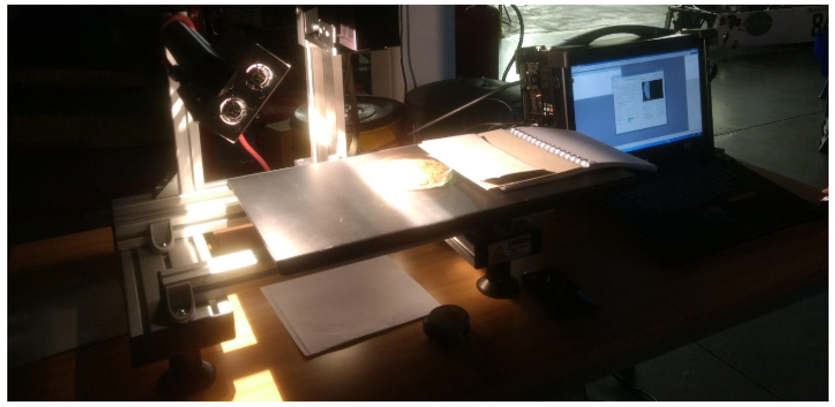
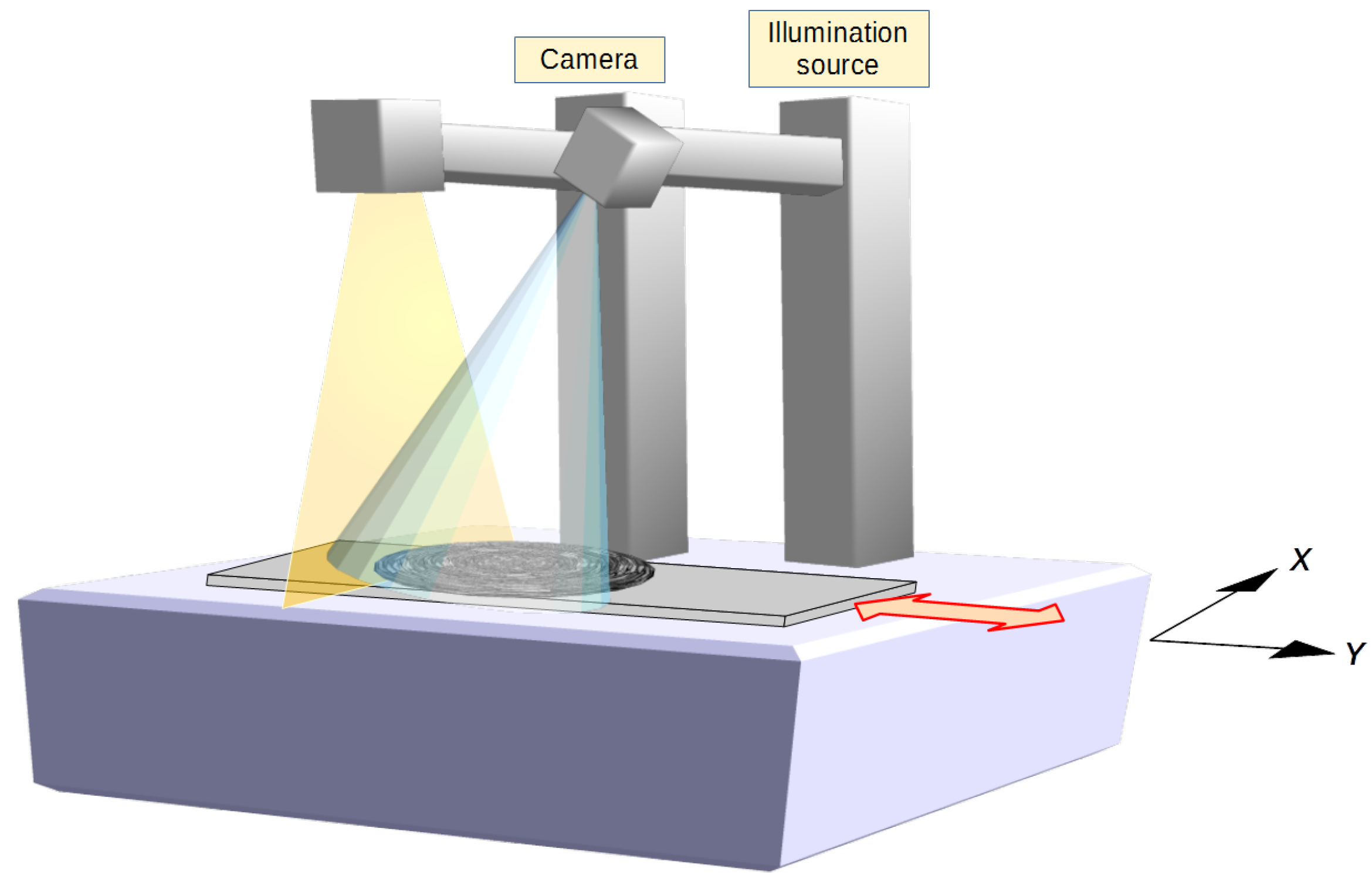
The spectral data was obtained using a Hyspex SWIR 384 m line-scan hyperspectral camera and is equipped with a Mercury Cadmium Telluride (MCT) detector array. For this experiment, a user friendly table-top laboratory set-up with translation stage, SWIR light source, and close-up lenses were used during the scanning stage to scan the sample and build a hyperspectral data cube (see Figure 2). The camera simultaneously captured a full SWIR spectrum, with a spectral sample interval of 5.45 nm between 930 and 2500 nm, each along a line of 384 pixels for 288 bands with a radiometric resolution of 16 bit [41]. The 384 columns of the detector array formed one line of the hyperspectral image in the x-axis. The hyperspectral image was obtained line by line using the so-called “pushbroom” scanning mode, where the platform holding the sample was translated onto the y-axis at constant speed (see Figure 3). The scanning speed was automatically controlled by the data acquisition unit based on the selected lens option. The images produced had a spatial resolution of $0.22$ mm/pixel. Radiometric calibration was performed using the vendor’s software package. A more detailed specification of the system is given in

Table 2. Hyspex 384 m main specifications.

Specification	HySpex SWIR-384 m
Spectral Range (nm)	930–2500
Spatial Pixels (pixels)	384
Spectral Channels	288
Spectral Sampling (nm)	5.45
FOV (degrees)	16°
Pixel FOV across/along (mrad)	0.73/0.73
Bit resolution (raw data)/Digitization	16
Noise floor ($e^{·}$)	150
Dynamic range	7500
Peak SNR (at full resolution)	>1100
Max speed (at full resolution)(fps)	400
Full Width Half Maximum	∼1 pixel
Power consumption (W)	30
Dimensions (l-w-h) (cm)	38-12-17.5
Weight (kg)	5.7

.

The resultant reflectance spectra were used to estimate the percentages of the HCs using the abundances calculated based on the different mixture types as shown in

Table 3. Size of datasets and target class.

Dataset	Size	Number of Mixtures
Clay biodiesel	$8000\times 288$	8
Clay diesel	$8000\times 288$	8
Clay ethanol	$8000\times 288$	8
Clay loam biodiesel	$7000\times 288$	7
Clay loam diesel	$7000\times 288$	7
Clay loam ethanol	$8000\times 288$	8
Clay loam petrol	$\mathrm{12,000}\times 288$	12
Sandy loam biodiesel	$5000\times 288$	5
Sandy loam diesel	$5000\times 288$	5
Sandy loam ethanol	$5000\times 288$	5
Sandy loam petrol	$\mathrm{10,000}\times 288$	10
Sandy clay loam biodiesel	$6000\times 288$	6
Sandy clay loam diesel	$6000\times 288$	6
Sandy clay loam ethanol	$7000\times 288$	7
Sandy clay loam petrol	$8000\times 288$	8

.

3. Methodology

3.1. Workflow

Spectral information was obtained from the controlled dataset and used with ground truth abundances to evaluate the performance of the proposed deep learning model for estimating the abundance of HCs in each dataset. The workflow of the study is as follows.

• Obtaining the dataset via a controlled experiment by mixing and homogenizing different Hydrocarbon (HC) types with soil samples and scanning them with a Hyspex Shortwave Infrared (SWIR) 384 m camera.
• Applying the Deep Learning (DL) model trained using a three-term backpropagation algorithm with dropout for the abundance estimation of the HCs.
• Structuring the DL model with different dropout ratios to determine the most efficient DL setting.
• Testing and validating the performance of the proposed method for abundance estimation of the different HCs by using the same network structure and hyperparameters.
• Comparing the accuracy and performance of the DL model with a hybrid spectral unmixing method [21] and DL models trained using a standard backpropagation algorithm with and without dropout (to prove the generalization ability of dropout), respectively.

The description and experimental results of this workflow are organized in the following sections. Further explanation and discussion regarding abundance estimation of the HCs by the DL model as well as the other methods can be found in the data acquisition, results, and discussion sections.

3.2. Deep Learning

Deep learning has been shown to outperform other machine learning and neural networks techniques. Deep learning can be categorized as a subfield of machine learning, which learns high level abstractions in data by utilizing hierarchical architectures [42]. Deep learning can also be described as the final product of machine learning where the learning rule becomes the algorithm that generates the model from the training data. It typically involves modeling, which hierarchically learn features of input data using Artificial Neural Networks (ANN) and usually has more than three layers [43]. The main advantage of deep learning is that these layers of features are not designed by an operator; they are learned from the input data using learning procedures. A deep neural network can simply be referred to as a network of sufficient complexity in order to interpret raw data without human derived explanatory variables [44,45]. Deep learning models provide excellent results with the ability to extract stronger features, but in turn lead to vanishing gradient, overfitting, and computational load [46]. These problems can be addressed and improved by employing dropout, three-term backpropagation and a Rectified Linear Unit (ReLU) activation function which is known to transmit error better when compared to other functions.

There are many types of deep learning architectures whose application have been proven to yield excellent results, the most common are Deep Believe Network (DBN), Convolutional Neural Network (CNN), Deep Convolutional Generative Adversarial Networks (DCGAN), Recurrent Neural Networks (RNN), etc. [47,48]. The application of deep learning techniques to hyperspectral data is relatively recent, for instance, in the work by the authors of [49], deep belief networks, and a novel texture enhancement algorithm were investigated for their suitability and practical application to hyperspectral image classification. The authors of [50] utilized high-resolution remote sensing imagery and deep learning techniques to extract buildings in urban districts using guided filters. In the work of the authors of [51], a 3D full convolutional neural network model was used for spatial-spectral resolution of hyperspectral images by learning end-to-end, with full mapping between low and high spatial resolution hyperspectral images at high accuracy. Transfer learning with a deep convolutional neural network was reported in the work by the authors of [52]; in this research, a large amount of unlabeled SAR scene data was transferred to SAR target recognition tasks with feedback of the construction loss to the classification pathway. Others, such as the authors of [53,54], used a deep learning approach to classify hyperspectral images. Most of the aforementioned methods used the standard backpropagation algorithm to train the network which has been characterized as having low convergence rates especially when used to train a network with more than one hidden layer. Thus, in this paper, the main aim of using the three-term backpropagation algorithm with dropout to train the network is to increase the convergence rate and the ability to generalize to unseen data with good prediction accuracy compared to existing methods.

3.3. Dropout

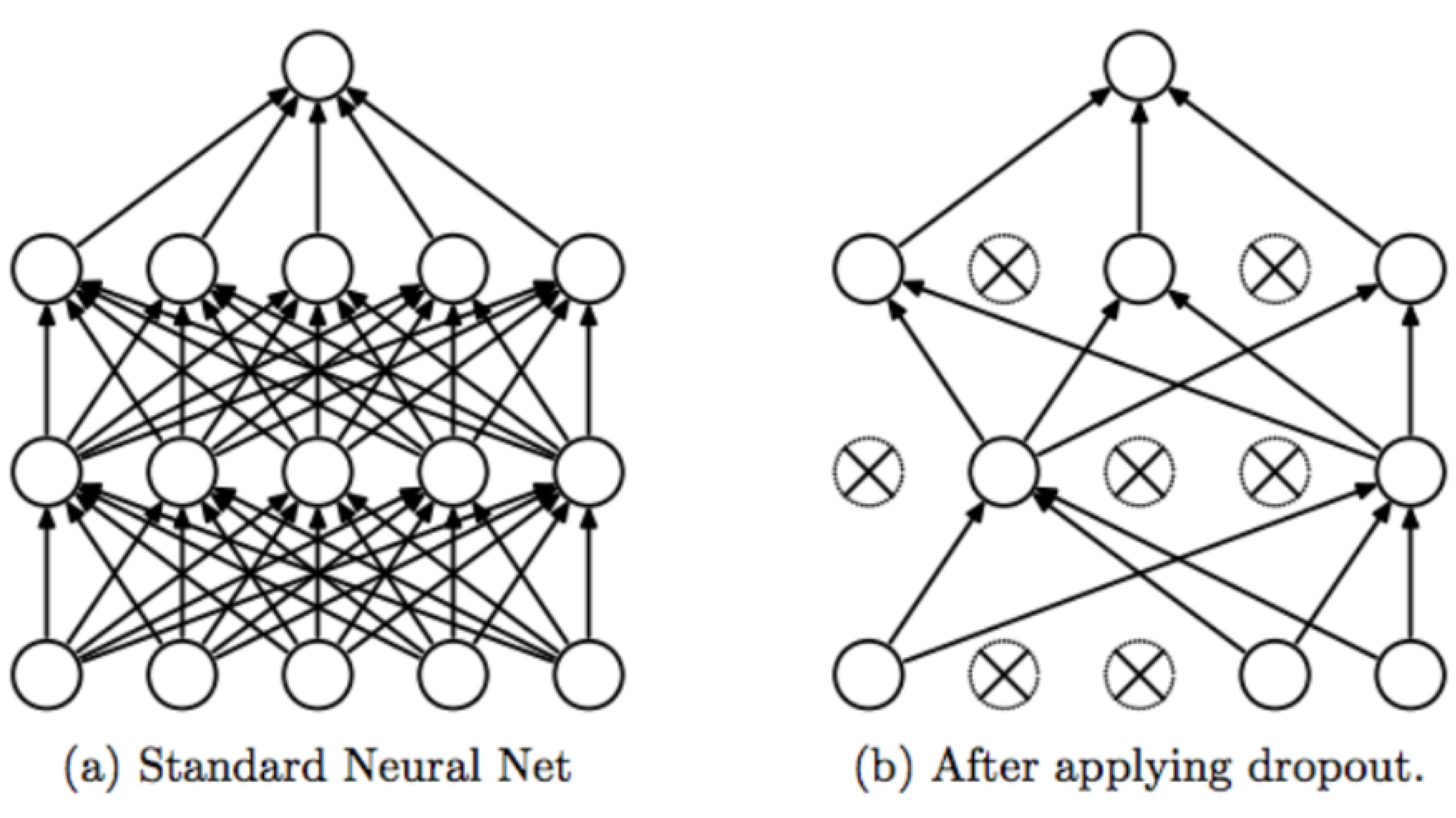
Dropout allows neurons to randomly drop out of the network during training, while other neurons can step in and handle the representation required to make predictions for the missing neurons [55]. This simply means removing neurons from the network along with all its incoming and out going connections. By applying dropout to a deep neural network, a thinned network often results. This thinned network consists of all the units that survive dropout [56] as shown in Figure 4. The dropout effect is that the network becomes less sensitive to the specific weights of neurons. This in turn results in a network that is capable of better generalization and is less likely to overfit the training data.

In this paper, dropout on hidden layers and on the visible layer are developed. Dropout on hidden layers is applied to hidden neurons in the hidden layers and between the last hidden layer and the output layer of the body of the deep networks’ model. Dropout on the visible layer is applied between the input and the first hidden layer. Since deep neural networks consist of multiple nonlinear hidden layers, this makes them expressive models that can learn complex relationships between the input and output nodes which often results in overfitting.

3.4. Backpropagation

Backpropagation is carried out to train multilayer architectures to minimize the cost function of the model. It is also used to adjust the free parameters weights ($\omega$) and biases in order to attain the desired network output. Traditionally, the learning rate and momentum factors are used to control the weight adjustments and damping oscillations. This is a popular training algorithm in many applications, however the main limitation is its slow convergence especially when used to train a deep neural network with multiple hidden layers. Therefore, the three-term backpropagation algorithm with dropout tend to improve the accuracy of the trained model.

3.5. Three-Term Backpropagation

The backpropagation algorithm has been modified by different researchers to improve the efficiency and convergence rate of the algorithm. One such method is the three-term backpropagation algorithm proposed by the authors of [57], shown in Algorithm 1. This algorithm uses an extra term called the Proportional Factor (PF) to the standard backpropagation algorithm. This PF speeds up the weight adjustment process by increasing the convergence rate and decreasing learning stalls while maintaining the simplicity and efficiency of the standard backpropagation algorithm [58].

Algorithm 1: Learning method using the three-term backpropagation with dropout used in training the DNN model.

Data: $\alpha$, $\beta$, $\gamma$, $\omega$, $\delta$, e  DNN weights, $\omega$, are randomly initialized ${\omega }_{11}$ ... ... ... ${\omega }_{ij}$  initialize the learning rate, $\alpha$; momentum factor, $\beta$; and proportional factor, $\gamma$

A stability analysis of the three-term backpropagation was studied in the work by the authors of [58] to test the convergence rate and stability of the algorithm. This training algorithm has proven to be effective in training a network with good prediction accuracy and a high convergence rate [58,59].

A deep learning model with dropout can be trained using the stochastic gradient descent which can be similar to a standard neural network, the only difference here is the random dropping of units in the network’s hidden layers. Different methods have been used to improve the standard gradient descent algorithm such as momentum, annealed learning rates, as well as L2 weight decay [55]. Here, the effectiveness of the dropout trained method using the three-term backpropagation algorithm is demonstrated. The three-term backpropagation algorithm speeds up weight space adjustment compared to a conventional backpropagation algorithm. The dropout has proven to be successful for computer vision tasks as it helps to avoid overfitting and improve generalization [60,61].

3.6. Hyperparameters

A deep learning model requires the modification of various hyperparameters in order to improve the results, and these largely depend on the dataset and other hyperparameters. The backpropagation algorithm involves two parameters in updating the weights during training which are: the learning rate ($\alpha$) and momentum factor ($\beta$).

The initial learning rate $\alpha$ is one of the most important hyperparameters; too small a learning rate makes the network learn slowly, and too large a learning rate possibly leads to oscillation preventing the error falling below a certain value.

The momentum factor $\beta$ is believed to make the learning procedure more stable and accelerate convergence in shallow regions of the error function, which in practice does not always happen [62].

The extra term introduced by the three-term back propagation algorithm, called the proportional factor ($\gamma$), speeds up the weight adjustment process by increasing the convergence rate and decreasing learning stalls of the algorithm.

The best choice of these parameters depends on the problem which often requires a trial and error process before a suitable choice is found [63]. Having run the experiments a number of times based on trial an error, the optimum values of the parameters were achieved which trained the network and output good results.

3.7. Architecture of the Deep Learning Model

The deep learning model was designed using the 288 bands as input to the network. Each pixel is taken as an independent input to the network. In this research study, we do not consider the spatial information. The network has four hidden layers each containing 30 nodes and one output corresponding to the abundance of hydrocarbon. The network was trained using the ground truth abundances for the different mixtures, as detailed in

Table 4. Ground truth abundances (expressed in $wt\%$) for the different mixtures corresponding to 2 mL, 4 mL, 5 mL, 10 mL, 15 mL, 20 mL, 25 mL, 30 mL, 35 mL, 40 mL, and 45 mL of HC , respectively.

Corresponding mixtures (mL)	Petrol	Diesel	Biodiesel	Ethanol
2.0	0.02	0.023	0.034	0.029
4.0	0.055	0.063	0.065	0.059
5.0	0.068	0.08	0.08	0.073
10.0	0.128	0.148	0.149	0.136
15.0	0.181	0.206	0.208	0.191
20.0	0.227	0.258	0.260	0.240
25.0	0.269	0.303	0.305	0.283
30.0	0.340	0.342	0.345	0.321
35.0	38.1	–	–	–
40.0	42.0	–	–	–
45.0	46.2	–	–	–

.

The data was randomly divided into 3 categories, namely: training, validation, and test sets. The training set is used to fit the parameters of the deep learning model, the test set (unseen data) is used to investigate the predictive power of the model while the validation set is used to avoid overfitting using the cross-validation algorithm.

The cross-validation algorithm avoids overfitting because the training sample is independent of the validation sample [64]. The size of the data sets depended on the soils’ absorption level during the experiment (i.e., when a local shallow pool was formed). Only image pixels corresponding to data from inside the Petri dish were considered. Moreover, for each scanned image, 1000 pixels were randomly selected. Thus the data sets ranged between 5000 pixels × 288 bands (where five mixture types were available) to 10,000 pixels × 288 bands (for samples with ten possible mixtures). The size of the data sets and number of mixtures used for the experiments (see Table 1) are summarized in Table 3. Subsets of the hyperspectral data were fed into the network as follows: 80% of the data were randomly selected for training the network, 10% were used to test the network and 10% were used for cross-validation.

We compared two neural network architectures one with and another without dropout, respectively. This is to prove the dropout’s efficiency to improve the generalization capabilities of the neural network.

The network used a sigmoid activation function which was applied to the hidden and output nodes.

The deep learning abundance estimation experiments were conducted to obtain optimum hyperparameters in order to achieve maximum accuracy in estimating the amount of HCs in each soil mixture type. The ground truth, or known abundances from the sample preparation, were used as class labels (targets) to train the network for the abundance estimation. These ground truth abundances were estimated based on the HC type in each data set as detailed in Table 4 and depend on the density of each HC.

All the experiments were conducted with the learning rate of $\alpha$ set to 0.01, $\beta$ set to 0.5, and $\gamma$ set to 0.1, which allowed convergence of the objective function at a high rate. The algorithm was run iteratively with 20 epochs.

Moreover, in order to find the optimum level of dropout, the models were trained using the three-term backpropagation algorithm with different ranges of dropout (10–50%).

4. Results

In this section, we present the results obtained from the deep learning model demonstrating the abundance estimation of the different HCs. Results are presented to demonstrate the effectiveness of dropout in the model in terms of generalization capabilities. We also show the accuracy of the proposed method compared to the hybrid spectral unmixing method and DL models trained with conventional backpropagation with and without dropout, respectively. Results with laboratory and remote sensed data are presented. The algorithms were implemented using MatLab 2018b. The experiments were carried out on an LG desktop with Intel (R) core ${\left(TM\right)}^2$ Duo CPU 3.00 GHZ processor 8.00 GB RAM.

4.1. Experiment with Laboratory Data

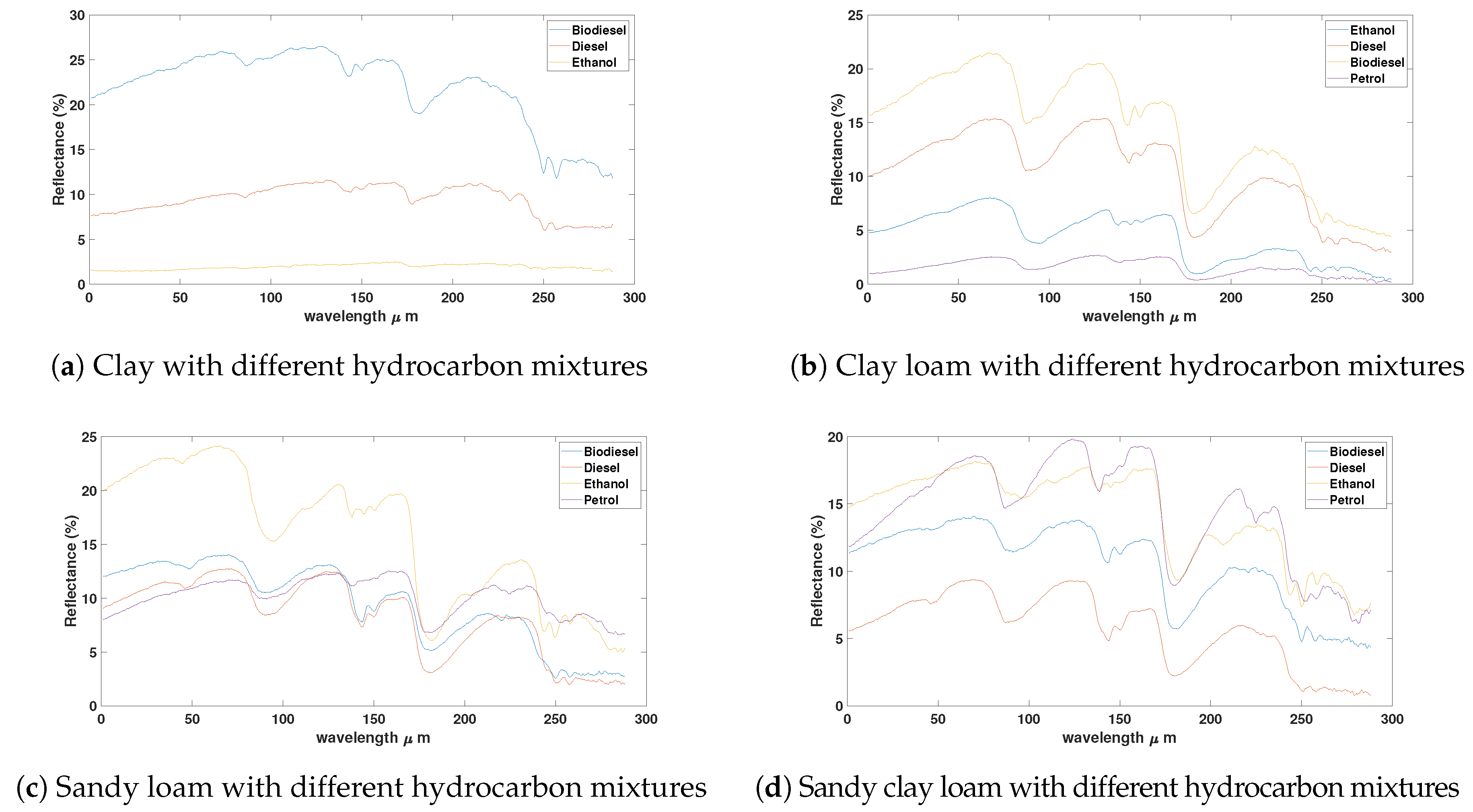
The reflectance spectra of different soil samples with $15\%$ hydrocarbon concentration mixture are shown in Figure 5 showing specific absorption at around 1700 μm and 2300 μm, respectively.

The ground truth abundances in Table 4 were used to estimate the amount of hydrocarbon used in the experiment. The abundances were calculated based on the density of the different hydrocarbon types. The aim is to quantify the percentage or amount of HC in each pixel using deep learning and hybrid spectral unmixing method (using abundance estimation). This was calculated based on the saturation level of the different hydrocarbons as shown in Table 1.

To demonstrate the ability of the proposed deep learning model to generalize on unseen data,

Table 5. Mean square error of the deep learning model on unseen data with and without dropout, respectively.

Dataset	Test Set with Dropout	Test Set without Dropout
Clay biodiesel	$7.11\times {10}^{-3}$	$9.1\times {10}^{-3}$
Clay diesel	$1.16\times {10}^{-3}$	$6.9\times {10}^{-3}$
Clay ethanol	$8.26\times {10}^{-4}$	$6.2\times {10}^{-3}$
Clay loam biodiesel	$7.62\times {10}^{-4}$	$1.4\times {10}^{-3}$
Clay loam diesel	$2.20\times {10}^{-3}$	$3.3\times {10}^{-3}$
Clay loam ethanol	$8.80\times {10}^{-4}$	$7.1\times {10}^{-3}$
Clay loam petrol	$2.50\times {10}^{-3}$	$8.1\times {10}^{-3}$
Sandy loam biodiesel	$8.00\times {10}^{-4}$	$1.2\times {10}^{-3}$
Sandy loam diesel	$1.20\times {10}^{-3}$	$9.8\times {10}^{-3}$
Sandy loam ethanol	$4.01\times {10}^{-3}$	$8.4\times {10}^{-3}$
Sandy loam petrol	$6.71\times {10}^{-3}$	$9.3\times {10}^{-3}$
Sandy clay loam biodiesel	$8.25\times {10}^{-4}$	$3.5\times {10}^{-3}$
Sandy clay loam diesel	$8.84\times {10}^{-4}$	$9.8\times {10}^{-3}$
Sandy clay loam ethanol	$2.10\times {10}^{-3}$	$7.5\times {10}^{-3}$
Sandy clay loam petrol	$5.13\times {10}^{-3}$	$6.1\times {10}^{-3}$

displays the results obtained from the test sets with and without dropout, respectively.

The experimental process was repeated with different dropout ratios on the hidden layers of 10%, 20%, 30%, 40%, and 50% respectively. Results demonstrate both the training and validation accuracy of the network.

Table 6. Mean Square Error (MSE) of the deep learning model for Clay Loam datasets with different hydrocarbon types and different Dropout (DO) ratios.

HC Types	DO 10%	DO 20%	DO 30%	DO 40%	DO 50%
Bio-diesel
MSE	$3.5\times {10}^{-4}$	$0.22\times {10}^{-4}$	$0.69\times {10}^{-4}$	$6.5\times {10}^{-4}$	$72\times {10}^{-4}$
Diesel
MSE	$0.31\times {10}^{-4}$	$0.25\times {10}^{-4}$	$0.52\times {10}^{-4}$	$7.3\times {10}^{-4}$	$59\times {10}^{-4}$
Ethanol
MSE	$3.1\times {10}^{-4}$	$0.21\times {10}^{-4}$	$5.6\times {10}^{-4}$	$74\times {10}^{-4}$	$76\times {10}^{-4}$
Petrol
MSE	$2.9\times {10}^{-4}$	$0.22\times {10}^{-4}$	$0.73\times {10}^{-4}$	$6.7\times {10}^{-4}$	$72\times {10}^{-4}$

,

Table 7. Mean square error of the deep learning model for Clay datasets with different hydrocarbon types and different Dropout (DO) ratios.

HC Types	DO 10%	DO 20%	DO 30%	DO 40%	DO 50%
Bio-diesel
MSE	$2.7\times {10}^{-4}$	$2.3\times {10}^{-4}$	$1.9\times {10}^{-4}$	$5.1\times {10}^{-4}$	$77\times {10}^{-4}$
Diesel
MSE	$1.7\times {10}^{-4}$	$0.35\times {10}^{-4}$	$1.7\times {10}^{-4}$	$3.2\times {10}^{-4}$	$76\times {10}^{-4}$
Ethanol
MSE	$1.6\times {10}^{-4}$	$2.2\times {10}^{-4}$	$2.8\times {10}^{-4}$	$4.3\times {10}^{-4}$	$83\times {10}^{-4}$

,

Table 8. Mean square error of the deep learning model for Sandy Clay Loam datasets with different hydrocarbon types and different Dropout (DO) ratios.

HC Types	DO 10%	DO 20%	DO 30%	DO 40%	DO 50%
Bio-diesel
MSE	$2.7\times {10}^{-4}$	$0.33\times {10}^{-4}$	$0.61\times {10}^{-4}$	$3.4\times {10}^{-4}$	$86\times {10}^{-4}$
Diesel
MSE	$2.7\times {10}^{-4}$	$2.0\times {10}^{-4}$	$5.3\times {10}^{-4}$	$6.6\times {10}^{-4}$	$94\times {10}^{-4}$
Ethanol
MSE	$3.4\times {10}^{-4}$	$2.2\times {10}^{-4}$	$4.3\times {10}^{-4}$	$7.2\times {10}^{-4}$	$88\times {10}^{-4}$
Petrol
MSE	$2.2\times {10}^{-4}$	$1.3\times {10}^{-4}$	$3.6\times {10}^{-4}$	$4.7\times {10}^{-4}$	$83\times {10}^{-4}$

and

Table 9. Mean square error of the deep learning model for Sandy Loam datasets with different hydrocarbon types and different Dropout (DO) ratios.

HC Types	DO 10%	DO 20%	DO 30%	DO 40%	DO 50%
Bio-diesel
MSE	$3.6\times {10}^{-4}$	$3.4\times {10}^{-4}$	$1.6\times {10}^{-4}$	$7.3\times {10}^{-4}$	$72\times {10}^{-4}$
Diesel
MSE	$2.7\times {10}^{-4}$	$0.2\times {10}^{-4}$	$0.66\times {10}^{-4}$	$3.1\times {10}^{-4}$	$68\times {10}^{-4}$
Ethanol
MSE	$2.5\times {10}^{-4}$	$0.2\times {10}^{-4}$	$7.3\times {10}^{-4}$	$5.8\times {10}^{-4}$	$86\times {10}^{-4}$
Petrol
MSE	$0.68\times {10}^{-4}$	$1.5\times {10}^{-4}$	$2.7\times {10}^{-4}$	$6.8\times {10}^{-4}$	$81\times {10}^{-4}$

illustrate the mean square error of the proposed method with the different dropout ratios. It is noted that in all cases the error is 10 times lower for dropout ratio of 40% than for 50%. Then again when the error drops significantly for dropout ratio 20%. However, when it is further reduced to 10%, the error increases. The 20% dropout is adopted subsequently in the rest of the experiments.

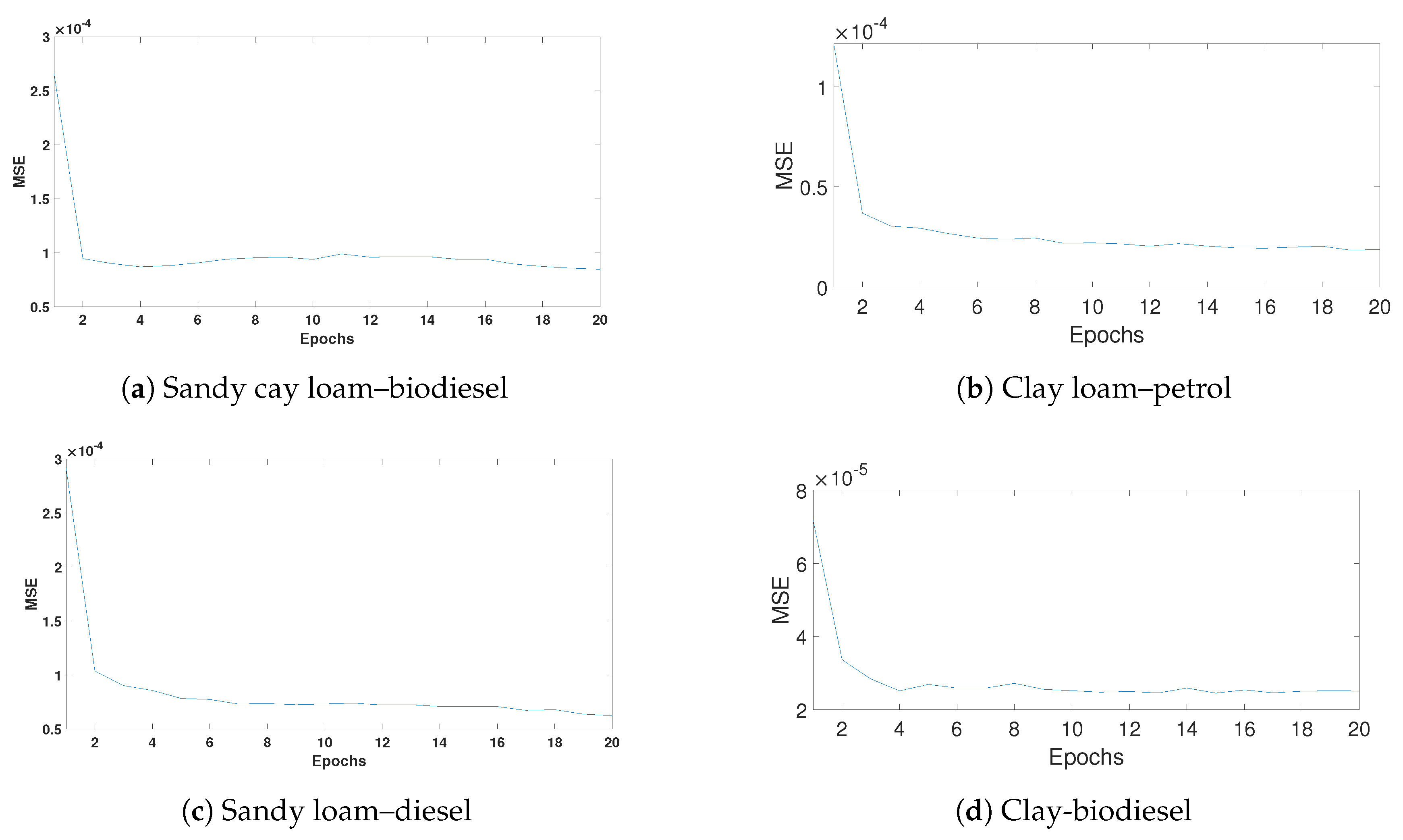
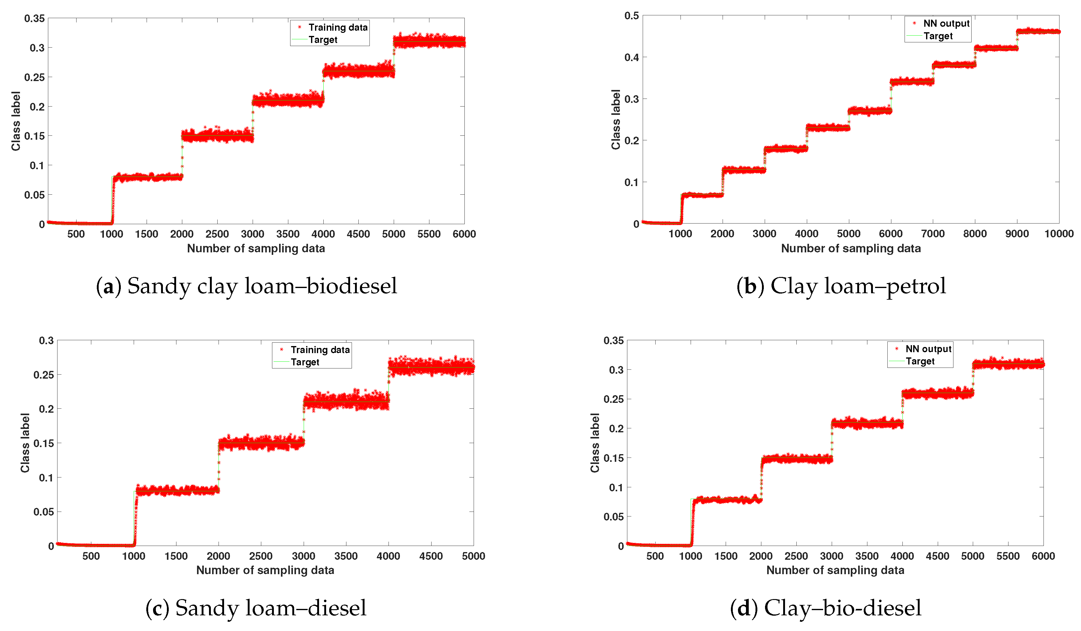
Results of the experiments are shown in Figure 6 and Figure 7 for individual soil types contaminated with different HCs to confirm the accuracy of the method. Figure 6 shows the mean square error during training, and demonstrates the network’s ability to converge rapidly with low numbers of epochs. The plots in Figure 7 show the model’s estimated output and target output for 4 different combinations. It is observed that the DL model quantifies correctly all the different HC abundances with low error.

From the results obtained, it is noted that the proposed method was able to generalize on unseen testing and validation data with high prediction accuracy. We observed a similar trend on all the datasets used for the experiment which indicates a reduction in the error rate and a high convergence rate.

To demonstrate the effectiveness of the proposed method, a deep learning model trained with a conventional backpropagation algorithm was similarly used to quantify the HC abundances; first without dropout, and then with 20 % dropout to train the networks. For fair comparison, the same network structure was used and these include: number of layers, number of nodes for each layer, range of initial values, and learning rate. Another comparison was conducted with the hybrid spectral unmixing method for switching between linear and nonlinear methods [21]. Hybrid spectral unmixing uses a neural network to determine the most appropriate method among a set of linear and non linear unmixing method for each pixel in the scene. Specifically, we used Vertex Component Analysis (VCA) [65], Fully Constrained Least Square Method (FCLS) [66], Generalized Bilinear Mixing Model (GBM) [67], and the Polynomial Post Nonlinear Mixing Model (PPNMM) [68]. This means that the hybrid switch method selects the best of these four methods for each pixel.

From the results obtained, it may be observed that our proposed method outperforms the hybrid switch method and conventionally trained networks with the closest estimate from the ground truth values as demonstrated in

Table 10. Estimated hydrocarbon abundance predicted by the proposed method, compared with the hybrid switch method, conventional neural network, and conventional neural network with dropout (DO) for Clay and Clay Loam (CL) mixtures. A comparative summary showing the average estimation error in percentage is included for each mixture type.

Mixtures	Reference	Proposed Method	Hybrid Switch Method	Conventionally Trained NN with DO (0.2)	Conventionally Trained NN
Clay–biodiesel	0	0.002	0.03	0.61	0.69
Clay–biodiesel	3	3.4	3.7	3.9	4.5
Clay–biodiesel	6	6.5	6.9	7.3	7.9
Clay–biodiesel	8	8.4	9.4	9.8	9.9
Clay–biodiesel	14.9	15.3	16.9	18.0	18.9
Clay–biodiesel	20.8	21.4	22.6	17.3	17.9
Clay–biodiesel	26.0	26.8	28.3	29.9	30.3
Clay–biodiesel	30.5	31.9	32.2	35.1	38.6
Average error (%)		2	10	17	20
Clay–diesel	0	0.003	0.04	1.06	1.79
Clay–diesel	3	3.3	3.7	4.6	4.9
Clay–diesel	6	6.5	6.3	6.9	7.21
Clay–diesel	8	8.1	7.6	4.8	3.7
Clay–diesel	14.8	15.3	13.0	19.1	19.8
Clay–diesel	20.6	21.4	18.5	23.8	25.5
Clay–diesel	25.8	25.6	23.6	29.1	29.4
Clay–diesel	30.3	30.6	32.2	36.1	37.7
Average error (%)		2	14	20	24
Clay–ethanol	0	0.004	0.05	1.41	2.04
Clay–ethanol	2	2.7	2.3	3.4	3.9
Clay–ethanol	5	5.5	5.3	6.01	6.63
Clay–ethanol	7.3	7.6	8.2	4.9	4.1
Clay–ethanol	13.6	14.1	15.6	10.4	9.9
Clay–ethanol	19.1	19.6	18.1	22.7	22.9
Clay–ethanol	24	24.9	22.9	27.7	28.3
Clay–ethanol	28.3	28.9	27.7	32.8	33.7
Average error (%)		3	9	19	23
CL–biodiesel	0	0.002	0.16	0.90	1.63
CL–biodiesel	3	3.2	3.6	4.5	4.9
CL–biodiesel	6	6.4	6.6	7.1	7.8
CL-biodiesel	8	8.5	7.7	9.9	10.8
CL-biodiesel	14.9	15.5	13.6	17.9	18.3
CL-biodiesel	20.8	21.6	18.7	24.6	24.9
CL-biodiesel	26.0	26.4	24.1	29.6	29.9
Average error (%)		2	11	17	21
CL-diesel	0	0.003	0.001	0.76	1.88
CL-diesel	3	3.3	3.1	3.7	4.3
CL-diesel	6	5.8	6.6	7.2	7.8
CL-diesel	8	8.4	10.4	11.6	11.9
CL-diesel	14.8	14.3	12.8	18.7	19.0
CL-diesel	20.6	21.1	22.1	24.4	25.3
CL-diesel	25.8	26.8	27.7	28.2	30.7
Average error (%)		3	13	26	31
CL-ethanol	0	0.002	0.05	1.22	1.79
CL-ethanol	2	2.4	2.7	3.6	3.9
CL-ethanol	5	5.2	5.4	5.9	6.4
CL-ethanol	7.3	7.6	6.7	9.6	9.9
CL-ethanol	13.6	14.4	11.6	16.7	17.0
CL-ethanol	19.1	19.7	18.5	22.6	22.9
CL-ethanol	24	24.6	25.9	26.7	27.5
CL-ethanol	28.3	28.7	29.9	30.7	31.2
Average error (%)		2	11	17	21
CL-petrol	0	0.002	0.006	0.36	1.40
CL-petrol	2	2.4	2.2	2.9	3.3
CL-petrol	5	5.1	5.5	6.3	6.9
CL-petrol	6.8	5.9	7.9	8.4	8.9
CL-petrol	12.8	12.9	13.0	11.0	9.9
CL-petrol	18.1	18.4	17.4	16.8	15.6
CL-petrol	22.7	23.1	24.4	19.8	18.5
CL-petrol	26.9	27.4	27.8	24.6	23.9
CL-petrol	34	34.9	35.6	29.7	29.8
CL-petrol	38.1	38.5	39.6	36.6	36.9
CL-petrol	42	42.4	44.4	38.3	36.1
CL-petrol	46.2	46.9	45.2	43.5	43.7
Average error (%)		1	5	13	16

and

Table 11. Soil continuity experiments. Mean square error of the bio-diesel deep learning model using generic models and individual models with added noise. Training and testing results are shown.

Dataset	Traning Data	Test Data
Biodiesel with generic model	7.2238 $\times {10}^{-4}$ ($1.525\times {10}^{-4}$)	$6.8\times {10}^{-3}$ ($2.374\times {10}^{-3}$)
Biodiesel with added noise
SNR (dB)	Traning data	Test data
40	$8.2117\times {10}^{-4}$	$8.9821\times {10}^{-4}$
30	$8.2594\times {10}^{-4}$	$8.9333\times {10}^{-4}$
20	$9.393\times {10}^{-4}$	0.001
10	$9.671\times {10}^{-4}$	0.001
Biodiesel with added noise on testing data
SNR (dB)	Training data	Test data
40	$6.9997\times {10}^{-4}$	$9.3811\times {10}^{-4}$
30	$6.9997\times {10}^{-4}$	$9.0321\times {10}^{-4}$
20	$6.9997\times {10}^{-4}$	$9.0657\times {10}^{-4}$
10	$6.9997\times {10}^{-4}$	$0.0012$

.

4.2. Soil Continuity Experiments

In this research, four different mixtures of soil were created and HC were added in discrete steps. However, in real life situations, both HC and soil levels of given samples are continuous rather than discrete. Therefore, in order to simulate a more realistic scenario, several strategies were explored. The first strategy was to create a generic model with all soils combined as opposed to separate models for each soil as in the previous experiments. It is noted that the soils were prepared and mixed manually and contained grains of different size (e.g., clay and sand mixture). By feeding the DL network with all types of soils, differences in the soil composition would appear from pixel to pixel. DLs were created including all four different soil mixtures (Clay, Clay–loam, Sandy loam, and Sandy clay–loam) rather than individually. Using the same architecture of the deep learning model, 80% of the resultant data was used to train the model, 10% was used as test sample and the remaining 10% was used for cross-validation. This was conducted to validate the network’s ability to estimate the amount of HC regardless of the soil type and allowing for different soil types. The results were in the same range as for the different HC. Table 11 summarizes the results obtained for biodiesel. It is noted the training MSE was in the same range as the individual model although the number of epochs required increased to 178. Average MSE for the individual models are shown in brackets for comparison purposes. The generalization MSE on the training data is higher than in the individual models. However, it is noticed that this data is more complex as the individual models as it contains four different soil types. In the work of the authors of [16], an individual model per soil type was recommended as the generic models degraded the responses. We believe that with further tuning of the hyperparameters, improved results could have been achieved. However, this is out of the scope of this paper.

In order to simulate a more realistic scenario, and following a similar approach presented in the work by the authors of [16], noise was added to the data to simulate continuous spectra values instead of discrete and also to evaluate the noise rejection of the models. Here, the datasets were corrupted with Random Gaussian noise with signal-to-noise ratio (SNR) ranging from 10 to 40 dB. The model shows similar performance even with low SNR, showing good noise rejection and accurate prediction at different ranges of SNR. For SNR lower than 20 dB, the generalization error deteriorates slightly. Initially, we added noise to the test data but not to the training, to simulate training with discrete samples and testing with continuous samples. The performance deteriorates for SNR = 10 dB, while for higher SNR, it is very stable showing good adaptation of the model to continuous spectra.

4.3. Experiment with Remote Sensed Data

A remote sensed data captured by an airborne system, adjusted to work under stationary condition in the field, was used to validate our proposed method. This dataset contains soils contaminated with different levels of hydrocarbon (between 0 to 10 $wt\%$ in steps of 1 $wt\%$) that were acquired at three different locations (Hamra, Kokhav, and Evrona) with a Hyper-Cam LW instrument. Each pixel responses are captured by 88 spectral bands in the spectral range of 8 to 12 μm with spectral resolution of 0.25 cm⁻¹. The experimental protocol, data capturing, and preprocessing of these datasets are fully described in the work by the authors of [16].

Each one of the 3 datasets was independently trained with a DL network. For each network, 75% of the samples were randomly selected for training and 25% were used for testing. These parameters were selected similar to the work by the authors of [16] in order to provide a fair comparison to the results they presented. A dropout ratio of 20% was used and all other hyperparameters were left as in our previous configuration. Results are presented as MSE for each dataset in

Table 12. Summary of the evaluation on the 3 different soils using the deep learning model trained with and without dropout.

Soil Type	MSE on Training Set	MSE on the Test Set
Hamra	$0.48\times {10}^{-4}$	$1\times {10}^{-4}$
Evona	$0.78\times {10}^{-4}$	$3.5\times {10}^{-4}$
Kokhav	$2\times {10}^{-4}$	$3\times {10}^{-4}$

. It was noted that our results surpassed in term of prediction accuracy the ones presented in the literature for these datasets. Moreover, the results show good generalization capabilities.

Results on all 3 datasets shows that our proposed DL method achieved acceptable results with consistent MSE values as shown in Figure 8c for both training and generalization.

5. Discussion

In this study, controlled hyperspectral datasets were used to assess the capabilities of the deep learning model to predict and quantify the amount of HC spills on different soil types. The deep learning approach was trained using a three-term backpropagation algorithm with dropout technique. The deep learning model designed for this experiment utilizes a sigmoid activation function and dropout of 20% in all the hidden layers of the architecture in order to avoid overfitting. Another advantage of utilizing dropout is its ability to generalize.

The main aim of the three-term backpropagation algorithm was to reduce the number of training epochs and maintain the system’s stability during training. Our proposed method was able to estimate the amount of HCs in each dataset with high accuracy using a low number of epochs. The network was able to achieve an average of $2.2\times {10}^{-4}$ mean square error on an average of 18 epochs as shown in Table 5, Table 6, Table 7 and Table 8 and Figure 6.

Dropout plays an important role in the architecture of the proposed deep learning model by improving the performance of the model and avoided overfitting on the training data. This can be proven from Table 5, where the results show the ability of the model to generalize on unseen data with good accuracy.

From the results obtained, it may be observed that hydrocarbon can be estimated even at low levels as shown in Table 10 and Table 11.

Table 10 and Table 11 summarize the abundance estimation of the quantity of HCs in the different mixture types using our proposed method, the hybrid spectral unmixing method, and the conventionally trained NN with and without dropout. For instance, if we observe the first mixture from Table 10 (biodiesel mixed with clay), it is noted that for pure clay sample (reference 0% HC), all methods provide very close estimate. The second raw presents the results for the same mixture with 8% of biodiesel, 92% of clay. Our proposed method estimated 8.4% of biodiesel with the hybrid switch method at 9.4%, while the neural network trained with a standard backpropagation algorithm with and without dropout estimated at 9.8% and 9.9%, respectively. Similar results were obtained for all the different samples as shown in Table 10 and Table 11.

In addition, the soil’s properties such as grain size and texture can lead to a variation in the absorption level, and thus the difference in detection of the different hydrocarbon types. The hybrid switch method was also able to estimate the amount of hydrocarbon spills with reasonable accuracy unlike the conventionally trained neural network which has low accuracy compared to the proposed method.

In the work by the authors of [69], it was revealed that deep learning requires large amounts of training data to achieve optimal performance and good generalization with minimum error. However, despite the size of the datasets used, the training process is faster with our proposed method, attributed to the use of the three-term backpropagation algorithm for training and the use of cross-validation with dropout. The authors of [55] reported that large neural networks trained in the standard way tend to overfit on small datasets. To see if dropout can improve this condition, we ran the experiment on all the datasets and varied the dropout ratio as shown in Table 6, Table 7, Table 8 and Table 9. From the results obtained, the error rate is relatively low when the dropout ratio is between 10% and 30%, with a slight increase when the ratio is set above 50%. Therefore, it can be concluded that dropout ratio between 10% and 30% provides an acceptable prediction estimation and could be used in any dataset for estimation analysis.

The proposed deep learning method was further validated on field datasets. In particular, the Hamra soils produced a better results with lower MSE of $0.48\times {10}^{-4}$ compared to the Kokhav and Evrona soils as shown in Figure 8c. This shows a similar trend to what was obtained in the work by the authors of [16]. Although the deep learning model did not estimate well abundances between 1 and 3 $wt$%, this could be attributed to the fact that the data was obtained within the Longwave Infrared Region (LWIR), which has a different spectral range with the laboratory controlled data used in this research. Nevertheless, our proposed deep learning model perform better with all 3 datasets in terms of MSE accuracy.

Recent research in deep learning suggests that a large dataset is required for training remote sensing data, which is a major drawback. This was not the case for our proposed model because the three-term backpropagation algorithm allows it to train faster using a minimum number of epochs to converge. The training process was relatively fast compared to standard networks where parameter updates are noisy in architectures with dropout. Learning takes an average of 28.16 seconds with our proposed deep learning model compared to the conventionally trained neural networks which takes an average of 300.68 seconds to learn. The data processing-to-end-product time of our proposed method is relatively more time-consuming compared to traditional spectral unmixing method, which is approximately 35.45 seconds compared to the hybrid spectral unmixing method which has an average of 24.64 seconds. This could be attributed to the number of parameters and training in the deep learning method compared to the spectral unmixing method.

However, we anticipate that including a wider range of data such as field HC leaks, will require larger datasets and longer training to account for the variability of the data. Nevertheless, the proposed methodology has proven to decrease significantly both the learning time and sample data required to achieve accurate generalization.

6. Conclusions

In this paper, we developed a deep learning approach to accurately estimate hydrocarbon spills on different soil samples measured using imaging spectroscopy. The deep learning model was trained using a three-term backpropagation algorithm with dropout. The aim was to improve the accuracy of the model, avoid overfitting, and converge faster.

Standard backpropagation algorithms build co-adaptation, which work well on training data but the network does not generalize to unseen data. Dropout neutralizes these co-adaptations by improving the network’s performance, thus enabling it to generalize. The choice of dropout ratio used in any neural network depends on the type of dataset and application.

The three-term backpropagation algorithm improves the network’s ability to train faster and overcome local minima when compared to conventional backpropagation algorithms. The effectiveness of the deep learning model was verified when tested on the datasets containing different soil samples mixed with different hydrocarbon types to estimate the amount of hydrocarbon spills in each dataset. The datasets were acquired using a Hyspex 384 SWIR camera under laboratory conditions. Many studies have shown the ability to detect HC using spectroscopy in the SWIR region. The results of the experiments consistently show that the proposed method provides high prediction accuracy with low error even for amounts of HC as low as 6.8%. Therefore, it can be concluded that the three-term backpropagation algorithm with dropout significantly improves the model’s operation.

The deep learning model was further applied on three datasets acquired with an airborne LWIR camera in field conditions which proved the effectiveness of the proposed method and its applicability in real world scenarios.

Satellite and airborne hyperspectral data with ground truth are expensive, thus making it difficult to obtain; but with the emergence of new lightweight sensors mounted on Unmanned Aerial Vehicles (UAV), the potential application of this research is very large. It is noted that data acquired in field conditions could be affected by several limitations such as variable illumination, atmospheric conditions, and sensor sampling distance which could affect the accuracy in using such dataset. However, in the work by the authors of [70], the correlation between datasets obtained under laboratory and outdoor conditions was demonstrated. Thus, a neural network could be trained with laboratory data and validated using remote UAV or airborne data. The information provided in this research study can be used as a guide to understand the potential and limitations of a hyperspectral sensor for HC abundance estimation.

Future work will develop networks that are able to classify and identify different types of HC incorporating also spatial information using convolutional neural networks.

References

- United Nations Environment Programme (UNEP). Environmental Assessment of Ogoniland; United Nations Environment Programme: Nairobi, Kenya, 2011; pp. 1–262. [Google Scholar]
- Raksuntorn, N.; Du, Q. A new linear mixture model for hyperspectral image analysis. In Proceedings of the 2008 IEEE International Geoscience and Remote Sensing Symposium, Boston, MA, USA, 7–11 July 2008; Volume 3, pp. III-258–III-261. [Google Scholar]
- Eweje, G. Environmental costs and responsibilities resulting from oil exploitation in developing countries: The case of the Niger Delta of Nigeria. J. Bus. Ethics 2006, 69, 27–56. [Google Scholar] [CrossRef]
- Latimer, J.S.; Zheng, J. The sources, transport, and fate of PAHs in the marine environment. PAHs Ecotoxicol. Perspect. 2003, 9. [Google Scholar] [CrossRef]
- Okparanma, R.N.; Mouazen, A.M. Determination of total petroleum hydrocarbon (TPH) and polycyclic aromatic hydrocarbon (PAH) in soils: A review of spectroscopic and nonspectroscopic techniques. Appl. Spectrosc. Rev. 2013, 48, 458–486. [Google Scholar] [CrossRef]
- Scafutto, R.D.M.; de Souza Filho, C.R.; de Oliveira, W.J. Hyperspectral remote sensing detection of petroleum hydrocarbons in mixtures with mineral substrates: Implications for onshore exploration and monitoring. ISPRS J. Photogramm. Remote Sens. 2017, 128, 146–157. [Google Scholar] [CrossRef]
- Salem, F.; Kafatos, M. Hyperspectral image analysis for oil spill mitigation. Paper presented at the 22nd Asian Conference on Remote Sensing, Taipei, Taiwan, 3–7 October 2011; Volume 5, p. 9. [Google Scholar]
- Okparanma, R.N.; Mouazen, A.M. Visible and near-infrared spectroscopy analysis of a polycyclic aromatic hydrocarbon in soils. Sci. World J. 2013, 2013, 160360. [Google Scholar] [CrossRef]
- Chakraborty, S.; Weindorf, D.C.; Li, B.; Ali, M.N.; Majumdar, K.; Ray, D. Analysis of petroleum contaminated soils by spectral modeling and pure response profile recovery of n-hexane. Environ. Pollut. 2014, 190, 10–18. [Google Scholar] [CrossRef]
- Lammoglia, T.; de Souza Filho, C.R. Spectroscopic characterization of oils yielded from Brazilian offshore basins: Potential applications of remote sensing. Remote Sens. Environ. 2011, 115, 2525–2535. [Google Scholar] [CrossRef]
- Fingas, M.; Brown, C. Oil spill remote sensing. In Earth System Monitoring; Springer: Berlin/Heidelberg, Germany, 2013; pp. 337–388. [Google Scholar]
- Clasen, A.; Somers, B.; Pipkins, K.; Tits, L.; Segl, K.; Brell, M.; Kleinschmit, B.; Spengler, D.; Lausch, A.; Förster, M. Spectral unmixing of forest crown components at close range, airborne and simulated Sentinel-2 and EnMAP spectral imaging scale. Remote Sens. 2015, 7, 15361–15387. [Google Scholar] [CrossRef]
- Scafutto, R.D.M.; de Souza Filho, C.R. Quantitative characterization of crude oils and fuels in mineral substrates using reflectance spectroscopy: Implications for remote sensing. Int. J. Appl. Earth Obs. Geoinf. 2016, 50, 221–242. [Google Scholar] [CrossRef]
- Pelta, R.; Ben-Dor, E. Assessing the detection limit of petroleum hydrocarbon in soils using hyperspectral remote-sensing. Remote Sens. Environ. 2019, 224, 145–153. [Google Scholar] [CrossRef]
- Webster, G.T.; Soriano-Disla, J.M.; Kirk, J.; Janik, L.J.; Forrester, S.T.; McLaughlin, M.J.; Stewart, R.J. Rapid prediction of total petroleum hydrocarbons in soil using a hand-held mid-infrared field instrument. Talanta 2016, 160, 410–416. [Google Scholar] [CrossRef]
- Pelta, R.; Ben-Dor, E. An Exploratory Study on the Effect of Petroleum Hydrocarbon on Soils Using Hyperspectral Longwave Infrared Imagery. Remote Sens. 2019, 11, 569. [Google Scholar] [CrossRef]
- Okparanma, R.N.; Coulon, F.; Mayr, T.; Mouazen, A.M. Mapping polycyclic aromatic hydrocarbon and total toxicity equivalent soil concentrations by visible and near-infrared spectroscopy. Environ. Pollut. 2014, 192, 162–170. [Google Scholar] [CrossRef] [Green Version]
- Schwartz, G.; Ben-Dor, E.; Eshel, G. Quantitative analysis of total petroleum hydrocarbons in soils: Comparison between reflectance spectroscopy and solvent extraction by 3 certified laboratories. Appl. Environ. Soil Sci. 2012, 2012, 751956. [Google Scholar] [CrossRef]
- Gholizadeh, A.; Saberioon, M.; Ben-Dor, E.; Boruuvka, L. Monitoring of selected soil contaminants using proximal and remote sensing techniques: Background, state-of-the-art and future perspectives. Crit. Rev. Environ. Sci. Technol. 2018, 48, 243–278. [Google Scholar] [CrossRef]
- Pabón, R.E.C.; de Souza Filho, C.R. Spectroscopic characterization of red latosols contaminated by petroleum-hydrocarbon and empirical model to estimate pollutant content and type. Remote Sens. Environ. 2016, 175, 323–336. [Google Scholar] [CrossRef]
- Ahmed, A.M.; Duran, O.; Zweiri, Y.; Smith, M. Hybrid spectral unmixing: Using artificial neural networks for linear/nonlinear switching. Remote Sens. 2017, 9, 775. [Google Scholar] [CrossRef]
- Xu, M.; Zhang, L.; Du, B.; Zhang, L.; Fan, Y.; Song, D. A mutation operator accelerated quantum-behaved particle swarm optimization algorithm for hyperspectral endmember extraction. Remote Sens. 2017, 9, 197. [Google Scholar] [CrossRef]
- Uezato, T.; Murphy, R.J.; Melkumyan, A.; Chlingaryan, A. A novel spectral unmixing method incorporating spectral variability within endmember classes. IEEE Trans. Geosci. Remote Sens. 2016, 54, 2812–2831. [Google Scholar] [CrossRef]
- Weeks, A.R. Fundamentals of Electronic Image Processing; SPIE Optical Engineering Press: Bellingham, WA, USA, 1996. [Google Scholar]
- Keshava, N.; Mustard, J.F. Spectral unmixing. IEEE Signal Process. Mag. 2002, 19, 44–57. [Google Scholar] [CrossRef]
- Drumetz, L.; Tochon, G.; Chanussot, J.; Jutten, C. Estimating the number of endmembers to use in spectral unmixing of hyperspectral data with collaborative sparsity. In Proceedings of the Submitted to the 13th International Conference on Latent Variable Analysis and Signal Separation (LVA-ICA), Grenoble, France, 21–23 February 2017; pp. 1–10. [Google Scholar]
- Hapke, B. Bidirectional reflectance spectroscopy: 1. Theory. J. Geophys. Res. Solid Earth 1981, 86, 3039–3054. [Google Scholar] [CrossRef]
- Dobigeon, N.; Tourneret, J.Y.; Richard, C.; Bermudez, J.; McLaughlin, S.; Hero, A.O. Nonlinear unmixing of hyperspectral images: Models and algorithms. Signal Process. Mag. IEEE 2014, 31, 82–94. [Google Scholar] [CrossRef]
- Halimi, A.; Altmann, Y.; Buller, G.S.; McLaughlin, S.; Oxford, W.; Clarke, D.; Piper, J. Robust unmixing algorithms for hyperspectral imagery. In Proceedings of the Sensor Signal Processing for Defence (SSPD), Edinburgh, UK, 22–23 September 2016; pp. 1–5. [Google Scholar]
- Liu, J.; Luo, B.D.S.C.J. Exploration of planetary hyperspectral images with unsupervised spectral unmixing: A case study of planet Mars. Remote Sens. 2018, 10, 737. [Google Scholar] [CrossRef]
- Zhang, X.; Li, C.; Zhang, J.; Chen, Q.; Feng, J.; Jiao, L.; Zhou, H. Hyperspectral Unmixing via Low-Rank Representation with Space Consistency Constraint and Spectral Library Pruning. Remote Sens. 2018, 10, 339. [Google Scholar] [CrossRef]
- Kang, S.; Xiurui, G.; Hairong, T. A new target detection method using nonlinear PCA for hyperspectral imagery. Bull. Surv. Mapp. 2015, 1, 105–108. [Google Scholar]
- Feng, D.C.; Chen, F.; Wen-Li, X. Detecting local manifold structure for unsupervised feature selection. Acta Autom. Sin. 2014, 40, 2253–2261. [Google Scholar] [CrossRef]
- Ahmed, A.; Duran, O.; Zweiri, Y.; Smith, M. Application of hybrid switch method to quantify oil spills. In Proceedings of the Hyperspectral Image and Signal Processing: Evolution in Remote Sensing (WHISPERS), Amsterdam, The Netherlands, 23–26 September 2018. [Google Scholar]
- Iordache, M.D.; Bioucas-Dias, J.M.; Plaza, A. Sparse unmixing of hyperspectral data. IEEE Trans. Geosci. Remote Sens. 2011, 49, 2014–2039. [Google Scholar] [CrossRef]
- Feng, J.; Rogge, D.; Rivard, B. Comparison of lithological mapping results from airborne hyperspectral VNIR-SWIR, LWIR and combined data. Int. J. Appl. Earth Obs. Geoinf. 2018, 64, 340–353. [Google Scholar] [CrossRef]
- Harris, J.; Rogge, D.; Hitchcock, R.; Ijewliw, O.; Wright, D. Mapping lithology in Canada’s Arctic: application of hyperspectral data using the minimum noise fraction transformation and matched filtering. Can. J. Earth Sci. 2005, 42, 2173–2193. [Google Scholar] [CrossRef]
- Rogge, D.; Rivard, B.; Segl, K.; Grant, B.; Feng, J. Mapping of NiCu–PGE ore hosting ultramafic rocks using airborne and simulated EnMAP hyperspectral imagery, Nunavik, Canada. Remote Sens. Environ. 2014, 152, 302–317. [Google Scholar] [CrossRef]
- Khamehchiyan, M.; Charkhabi, A.H.; Tajik, M. Effects of crude oil contamination on geotechnical properties of clayey and sandy soils. Eng. Geol. 2007, 89, 220–229. [Google Scholar] [CrossRef]
- Soil Survey Division Staff. Soil Survey Manual; Number 18; Government Printing Office: Washington, DC, USA, 1993.
- Mathieu, M.; Roy, R.; Launeau, P.; Cathelineau, M.; Quirt, D. Alteration mapping on drill cores using a HySpex SWIR-320m hyperspectral camera: Application to the exploration of an unconformity-related uranium deposit (Saskatchewan, Canada). J. Geochem. Explor. 2017, 172, 71–88. [Google Scholar] [CrossRef]
- Guo, Y.; Liu, Y.; Oerlemans, A.; Lao, S.; Wu, S.; Lew, M.S. Deep learning for visual understanding: A review. Neurocomputing 2016, 187, 27–48. [Google Scholar] [CrossRef]
- Chen, Y.; Lin, Z.; Zhao, X.; Wang, G.; Gu, Y. Deep learning-based classification of hyperspectral data. IEEE J. Sel. Top. Appl. Earth Obs. Remote Sens. 2014, 7, 2094–2107. [Google Scholar] [CrossRef]
- LeCun, Y.; Bengio, Y.; Hinton, G. Deep learning. Nature 2015, 521, 436–444. [Google Scholar] [CrossRef]
- Ayrey, E.; Hayes, D.J. The Use of Three-Dimensional Convolutional Neural Networks to Interpret LiDAR for Forest Inventory. Remote Sens. 2018, 10, 649. [Google Scholar] [CrossRef]
- Kim, P. Deep Learning. In MATLAB Deep Learning: With Machine Learning, Neural Networks and Artificial Intelligence; Springer: New York, NY, USA, 2017; pp. 103–120. [Google Scholar]
- Gallego, A.J.; Pertusa, A.; Gil, P. Automatic Ship Classification from Optical Aerial Images with Convolutional Neural Networks. Remote Sens. 2018, 10, 511. [Google Scholar] [CrossRef]
- Jin, X.; Jie, L.; Wang, S.; Qi, H.J.; Li, S.W. Classifying Wheat Hyperspectral Pixels of Healthy Heads and Fusarium Head Blight Disease Using a Deep Neural Network in the Wild Field. Remote Sens. 2018, 10, 395. [Google Scholar] [CrossRef]
- Li, J.; Xi, B.; Li, Y.; Du, Q.; Wang, K. Hyperspectral Classification Based on Texture Feature Enhancement and Deep Belief Networks. Remote Sens. 2018, 10, 396. [Google Scholar] [CrossRef]
- Xu, Y.; Wu, L.; Xie, Z.; Chen, Z. Building extraction in very high resolution remote sensing imagery using deep learning and guided filters. Remote Sens. 2018, 10, 144. [Google Scholar] [CrossRef]
- Mei, S.; Yuan, X.; Ji, J.; Zhang, Y.; Wan, S.; Du, Q. Hyperspectral image spatial super-resolution via 3D full convolutional neural network. Remote Sens. 2017, 9, 1139. [Google Scholar] [CrossRef]
- Huang, Z.; Pan, Z.; Lei, B. Transfer learning with deep convolutional neural network for SAR target classification with limited labeled data. Remote Sens. 2017, 9, 907. [Google Scholar] [CrossRef]
- Wu, H.; Prasad, S. Convolutional recurrent neural networks for hyperspectral data classification. Remote Sens. 2017, 9, 298. [Google Scholar] [CrossRef]
- Fu, G.; Liu, C.; Zhou, R.; Sun, T.; Zhang, Q. Classification for high resolution remote sensing imagery using a fully convolutional network. Remote Sens. 2017, 9, 498. [Google Scholar] [CrossRef]
- Srivastava, N.; Hinton, G.; Krizhevsky, A.; Sutskever, I.; Salakhutdinov, R. Dropout: A simple way to prevent neural networks from overfitting. J. Mach. Learn. Res. 2014, 15, 1929–1958. [Google Scholar]
- Brownlee, J. Deep Learning with Python: Develop Deep Learning Models on Theano and TensorFlow Using Keras; Machine Learning Mastery: Vermont Victoria, Australia, 2016. [Google Scholar]
- Zweiri, Y.H.; Whidborne, J.F.; Althoefer, K.; Seneviratne, L.D. A new three-term backpropagation algorithm with convergence analysis. In Proceedings of the IEEE International Conference on Robotics and Automation (ICRA’02), Washington, DC, USA, 11–15 May 2002; Volume 4, pp. 3882–3887. [Google Scholar]
- Zweiri, Y.H.; Seneviratne, L.D.; Althoefer, K. Stability analysis of a three-term backpropagation algorithm. Neural Netw. 2005, 18, 1341–1347. [Google Scholar] [CrossRef]
- Zweiri, Y.H.; Whidborne, J.F.; Seneviratne, L.D. Optimization and stability of a three-term backpropagation algorithm. In Proceedings of the International Conference of Neural Networks (CI’2000), Como, Italy, 23–27 July 2000. [Google Scholar]
- Dahl, G.E.; Sainath, T.N.; Hinton, G.E. Improving deep neural networks for LVCSR using rectified linear units and dropout. In Proceedings of the 2013 IEEE International Conference on Acoustics, Speech and Signal Processing (ICASSP), Vancouver, BC, Canada, 26–31 May 2013; pp. 8609–8613. [Google Scholar]
- Maas, A.L.; Hannun, A.Y.; Ng, A.Y. Rectifier nonlinearities improve neural network acoustic models. In Proceedings of the International Conference on Machine Learning (ICML 2013), Atlanta, GA, USA, 16–21 June 2013; Volume 30, p. 3. [Google Scholar]
- Riedmiller, M.; Braun, H. A direct adaptive method for faster backpropagation learning: The RPROP algorithm. In Proceedings of the IEEE International Conference on Neural Networks, San Francisco, CA, USA, 28 March–1 April 1993; pp. 586–591. [Google Scholar]
- Abdulkadir, S.J.; Shamsuddin, S.M.; Sallehuddin, R. Three term back propagation network for moisture prediction. In Proceedings of the International Conference on Clean and Green Energy, Hong Kong, China, 5 January 2012; pp. 103–107. [Google Scholar]
- Arlot, S.; Celisse, A. A survey of cross-validation procedures for model selection. Stat. Surv. 2010, 4, 40–79. [Google Scholar] [CrossRef]
- Nascimento, J.M.; Dias, J.M.B. Vertex component analysis: A fast algorithm to unmix hyperspectral data. IEEE Trans. Geosci. Remote Sens. 2005, 43, 898–910. [Google Scholar] [CrossRef]
- Heinz, D.C. Fully constrained least squares linear spectral mixture analysis method for material quantification in hyperspectral imagery. IEEE Trans. Geosci. Remote Sens. 2001, 39, 529–545. [Google Scholar] [CrossRef] [Green Version]
- Altmann, Y. Nonlinear spectral unmixing of hyperspectral images. Ph.D. Thesis, l’Institut National Polytechnique de Toulouse (INP Toulouse), Toulouse, France, 2013. [Google Scholar]
- Altmann, Y.; Halimi, A.; Dobigeon, N.; Tourneret, J.Y. Supervised nonlinear spectral unmixing using a postnonlinear mixing model for hyperspectral imagery. IEEE Trans. Image Process. 2012, 21, 3017–3025. [Google Scholar] [CrossRef]
- Krizhevsky, A.; Sutskever, I.; Hinton, G.E. Imagenet classification with deep convolutional neural networks. In Proceedings of the Advances in Neural Information Processing Systems, Lake Tahoe, CA, USA, 3–6 December 2012; pp. 1097–1105. [Google Scholar]
- Crucil, G.; Castaldi, F.; Aldana-Jague, E.; van Wesemael, B.; Macdonald, A.; Van Oost, K. Assessing the Performance of UAS-Compatible Multispectral and Hyperspectral Sensors for Soil Organic Carbon Prediction. Sustainability 2019, 11, 1889. [Google Scholar] [CrossRef]
Figure 1.
Sample preparation of the experiment combining sandy-clay-loam with diesel. Photos show the HC contaminant being increasingly added to the same soil sample until saturated. From left; addition of 5 mL , followed by 10 mL, 15 mL, 20 mL, and 25 mL of the HC.
Figure 2.
Scanning process of the dataset.
Figure 3.
HySpex 384 m line scan acquisition process. The camera (nadir) acquires hyperspectral lines of pixels. The hyperspectral image is obtained by translation of the object under constant illumination.
Figure 4.
(a) A typical network before and (b) after applying dropout (adapted from the work by the authors of [55]).
Figure 5.
Spectral reflectance of different soils and hydrocarbon concentration mixtures.Clay mixtures.
Figure 6.
Mean square error of different soils contaminated with different HC contents.
Figure 7.
Neural network estimated output and target output of different soils contaminated with different HC contents.
Figure 8.
Mean square error of the 3 different soils contaminated with different HC contents.