Pattern Statistics Network for Classification of High-Resolution SAR Images


1
Electronic Information School, Wuhan University, Wuhan 430072, China
2
State Key Laboratory for Information Engineering in Surveying, Mapping and Remote Sensing, Wuhan University, Wuhan 430079, China
3
Collaborative Innovation Center of Geospatial Technology, 129 Luoyu Road, Wuhan 430079, China
*
Author to whom correspondence should be addressed.
Remote Sens. 2019, 11(16), 1942; https://0-doi-org.brum.beds.ac.uk/10.3390/rs11161942
Submission received: 1 July 2019
/
Revised: 14 August 2019
/
Accepted: 16 August 2019
/
Published: 20 August 2019
(This article belongs to the Section Remote Sensing Image Processing)
Abstract
:The classification of synthetic aperture radar (SAR) images is of great importance for rapid scene understanding. Recently, convolutional neural networks (CNNs) have been applied to the classification of single-polarized SAR images. However, it is still difficult due to the random and complex spatial patterns lying in SAR images, especially in the case of finite training data. In this paper, a pattern statistics network (PSNet) is proposed to address this problem. PSNet borrows the idea from the statistics and probability theory and explicitly embeds the random nature of SAR images in the representation learning. In the PSNet, both fluctuation and pattern representations are extracted for SAR images. More specifically, the fluctuation representation does not consider the rigorous relationships between local pixels and only describes the average fluctuation of local pixels. By contrast, the pattern representation is devoted to hierarchically capturing the interactions between local pixels, namely, the spatial patterns of SAR images. The proposed PSNet is evaluated on three real SAR data, including spaceborne and airborne data. The experimental results indicate that the fluctuation representation is useful and PSNet achieves superior performance in comparison with related CNN-based and texture-based methods.

1. Introduction
Synthetic aperture radar (SAR) has been used in a wide range of remote sensing applications for many years because it provides many unique advantages, such as day-and-night acquisition, certain penetrability, and polarimetric capability [1,2]. With the development of SAR sensors, e.g., TerraSAR-X [3], RADARSAT-2 [4], Sentinel-1 [5], and Gaofen-3 [6], large amounts of SAR images have become available and the automatic interpretation of such massive data has been an active research topic. This paper deals with the classification of single-polarized SAR image, which is one of the fundamental problems in the automatic interpretation task [7,8,9,10]. In recent years, the classification techniques based on convolutional neural networks (CNNs) [11] have drawn a lot of attention in the remote sensing community. Significant efforts have been made to shift to this paradigm [12,13].
1.1. Motivation and Objective
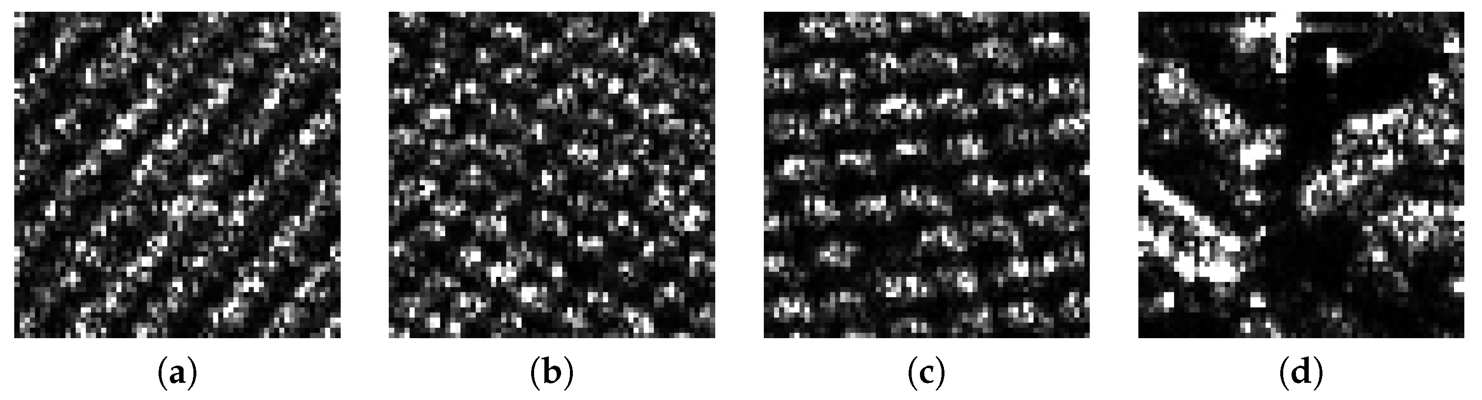
The CNN-based classification methods mainly depend on the representation learning by which data representations are automatically extracted to make it easier to perform the classification task [14,15]. However, it still remains a challenge in representation learning to identify the random and ever-changing patterns lying in SAR data, especially in the case of finite training data. The convolution in CNNs is basically a type of inner product in the Euclidean space [16], and it is equivalent to the matched filtering [17]. For example, the response (or feature) of the convolutional transformation to an image reflects the underlying spatial patterns of this image. For the SAR images, the above matched filtering becomes difficult because the spatial patterns are random and ever-changing, as shown in Figure 1. In this context, to cover the varying spatial patterns, the degrees of freedom of CNNs need to be increased, which in turn requires a large amount of training data. However, the lack of training data in SAR remote sensing is a common problem. In fact, the backscattered echoes in SAR are always varying because of the coherent imaging mechanism [18], and therefore collecting enough training samples may be intractable.
The effective representation should capture the underlying explanatory factors of the observed data for a specific task [15,19]. It is widely believed that the specific domain knowledge of the data plays an important role in helping to design effective data representation [15,20]. For the SAR image, its chaotic and unordered appearance indicates that it is a type of statistical signal. Therefore, its statistics are potentially useful for data representation [21,22]. For example, most of the traditional methods are based on the statistical analysis, and the first- and second-order statistics of SAR image have been widely used for data representation [23,24]. For example, the mean and standard deviation of SAR image do not consider the rigorous relationships between local pixels, and they can be regarded as the fluctuation representations of SAR image. Since the average operation is used to calculate the order statistics, the high variability of SAR image is significantly weakened. Figure 2 illustrates such a scatter plot. It can be observed that the high intra-class variations of SAR images become non-salient. Therefore, the objective of this paper lies in: embedding the statistical properties of SAR images in the representation learning to make it easier to perform the classification task.
1.2. Contribution
This paper explicitly makes use of the statistical nature of the SAR image in the representation learning. The proposed pattern statistics network (PSNet) has two sub-nets, including a discriminative net (DiscNet) and a pattern net (PatterNet). In the PSNet, both fluctuation and pattern representations are learned to describe an SAR image:
- The fluctuation representation is derived from SAR image statistics, including the mean and standard deviation. These image statistics are adaptively mapped into a high-dimensional space by the DiscNet to fit discriminative fluctuation representation. The fluctuation representation does not consider the rigorous relationships between local pixels, and only describes the average fluctuation of local pixels.
- In contrast to the fluctuation representation, the pattern representation, which are automatically extracted by the PatterNet, devotes to hierarchically capturing the relationships between local pixels, namely, the spatial patterns lying in SAR images.
The contributions of the fluctuation representation and pattern representation to the final representation of SAR image are learned by minimizing the classification error.
The proposed PSNet is distinguished from other CNN-based methods in that it explicitly integrates the statistical mechanism of SAR image into the representation learning. The representation extracted by the PSNet not only describes the relationships between local pixels, but also captures the average fluctuations of local pixels from a global view.
2. Related Work
A wide variety of methods for SAR image representation have been proposed. These methods can be divided into three categories: statistical models, textural analysis, and deep neural networks. This section briefly reviews the related works from which this paper draws inspiration.
2.1. Statistical Model
The chaotic and unordered appearance of speckle patterns bears no obvious relationships to the properties of illuminated objects, and most of the traditional works are based on the statistical analysis. In this line of work, the primary goal is to model the joint distribution of the texture and speckle random variables in the so-called multiplicative model [24]. In the case of fully developed speckle pattern, Gaussian assumption is valid [25]. That is, the real and imaginary parts of the backscattered signal are independent and identically distributed Gaussian variables [21]. Therefore, the exponential distribution and the gamma distribution can be respectively derived from this assumption for single-look and L-look intensity SAR images [21,26]. As the resolution increases, more details of the illuminated objects can be resolved, but the Gaussian assumption does not hold anymore [27]. In this case, the speckle patterns are partially developed, and therefore the statistical models should account for the texture variable. Many statistical models have been proposed for the high-resolution SAR images, such as Weibull, Log-Normal, and distribution [28,29]. These statistical distributions have shown success in modelling high-resolution SAR images. However, they are not flexible enough to fit different types of non-Gaussian SAR images, since these models have limited degrees of freedom. Therefore, to further increase the flexibility of the statistical models, researchers have proposed the compound and mixture probability models, such as generalized compound probability model [30], Fisher distribution [7], Gamma mixture model [31], and generalized Gamma mixture model (GMM) [32]. The basic idea behind the statistical model is to capture the statistical properties of SAR image. This idea inspires the proposed PSNet which explicitly considers the statistical properties of SAR image in the representation learning.
2.2. Texture Analysis
Texture is probably the most important feature used for describing the spatial variations of SAR images. A considerable amount of research has been dedicated to texture analysis, which can be roughly categorized into statistical, geometrical, model-based, and signal processing methods [33]. The statistical methods take the random variation of texture into account and extract a set of textural features based on the assumption that the textural information of SAR images exists in an “average” way. For example, textural features extracted by the statistical methods have been suggested for SAR image analysis in [23], and these features have been demonstrated to be effective in the classification task. However, the multiplicative property of speckle was not considered for the texture modelling in [23]. Ulaby et al. subsequently proposed a multiplicative model from which the second-order statistics of texture were derived [24], and textural features based on the second-order grey-level co-occurrence matrix (GLCM) [34] were applied to the classification of SAR images. In 2010, Esch et al. [35] used the concept of heterogeneity to describe the local development of speckle patterns. With this concept, the deviations of partially developed speckle patters from the fully developed speckle are measured with a series of thresholds, and these deviations are used for SAR image segmentation. This idea was further extended in [8] where the coefficient of variations of texture was estimated and its statistical characteristics were applied to SAR image classification. The geometrical methods borrow the idea from human visual perception and regard the texture as a superposition of a set of primitives, or the so-called textons [36]. The spatial layouts of these primitives are governed by the unordered and ordered rules, such as bag-of-features (BoF) [37] and spatial pyramid matching (SPM) [38]. The model-based methods believe that the texture is a realization of a generative model. Generally, the connections between local pixels are modeled by the Markovian framework [39,40], such as Hidden Markov Random Fields (HMRF) [41], Gaussian Markov Random Fields (GMRF) [42], and Lognormal Random Fields [43]. The signal processing methods analyze the texture from the perspective of frequency components [44]. The textural features are extracted with a bank of filters and multi-scale processing is generally used, e.g., Gabor filtering and Wavelet transforms [45,46,47]. The aforementioned methods use hand-crafted features to describe the texture information. By contrast, the presented PSNet integrates SAR image statistics into the representation learning and describes the texture with the learned features.
2.3. Deep Neural Networks
Deep neural networks automatically discover representations for SAR image with multiple processing layers. They generally fall into two categories: the deep generative and the deep discriminative networks [48,49]. The deep generative networks, such as deep Boltzmann machines (DBM) [50] and deep belief networks (DBN) [51], are devoted to learning and approximating the true distribution of SAR images [33] with hierarchical architectures. Liu et al. proposed Wishart–Bernoulli DBN (WDBN) for Polarimetric SAR imagery classification, where the conditional probabilities between the visible and hidden units were modeled by the Wishart and Bernoulli distributions [52]. In [53], the DBM model was used for SAR image classification, and it achieved higher classification accuracy than traditional methods on RADARSAT-2 data. Gao et al. combined DBN with the ensemble learning to extract discriminant features for SAR images, and they obtained promising classification performance [54]. In particular, the latest proposed generative adversarial networks (GAN) [55] have shown success in data generation, which is expected to be extended to SAR image interpretation. For the deep discriminative networks, they exploit the hierarchical architectures to directly predict the classification probability. A variety of deep discriminative networks have been proposed, such as standard CNNs [11], deep residual network (ResNet) [56], densely connected convolutional network (DenseNet) [57], and spatial pyramid pooling deep convolutional network (SPPNet) [58]. Several deep discriminative networks have been applied to SAR image classification. A deep supervised and contractive neural network (DSCNN) was presented to extract primitive features for SAR image classification [59,60]. Standard CNNs and complex-valued CNNs were proposed for PolSAR imagery classification, where both polarimetric and spatial features of PolSAR data were exploited [61,62]. Deep memory convolution neural network (M-Net) resorts to the information recorder to alleviate the overfitting problem in SAR image classification [63]. The above methods rely on the representation learning to extract features for SAR images, while the proposed PSNet integrates the inherent statistical mechanism of SAR data into the representation learning. The representations extracted by the PSNet not only capture the spatial patterns lying in SAR image, but also describe the statistical properties of SAR images.
3. Methodology
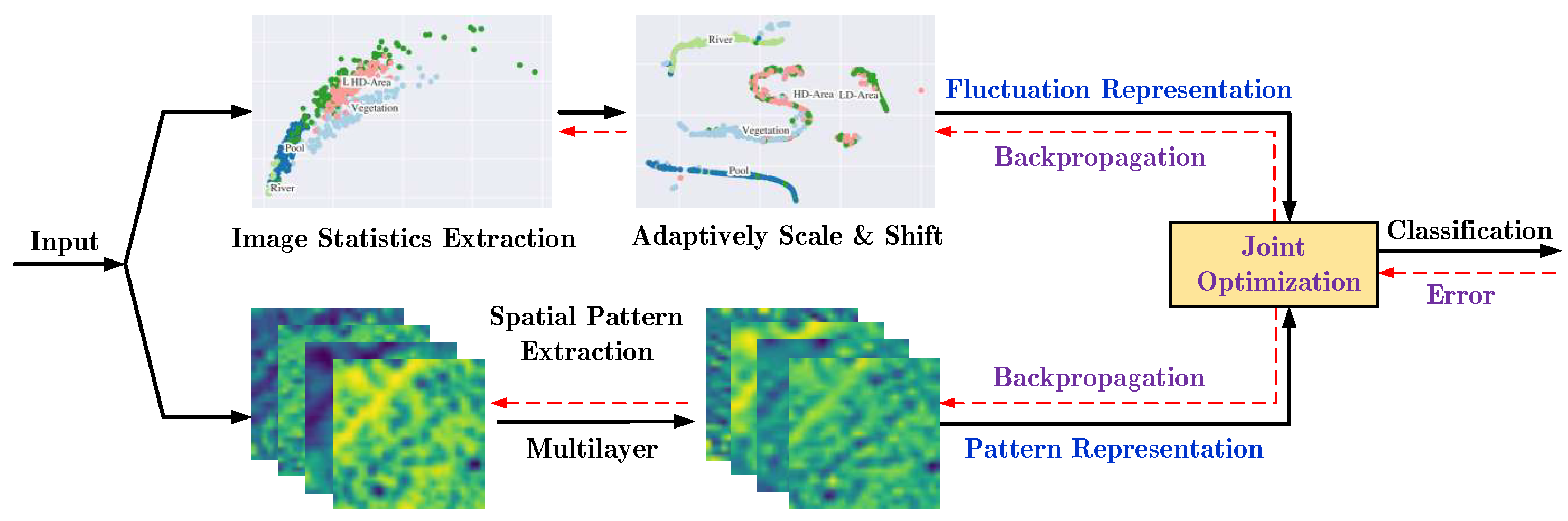
Figure 3 illustrates the framework of PSNet by which both the fluctuation and pattern representations of the input can be jointly learned. The fluctuation representation, deriving from the input statistics, does not consider the interactions between local pixels and only describes the average fluctuation of the input. By contrast, the pattern representation hierarchically captures the relationships between local pixels, namely, the spatial pattern lying in the input.
In the following subsections, firstly, the statistical behavior of SAR image is briefly reviewed and the fluctuation representation of SAR image is explained. Secondly, the proposed PSNet is described in detail. Finally, the optimization of PSNet is presented.
3.1. Statistical Behavior of SAR Images
SAR images are characterized by its unordered and granular appearance known as speckle, which is generally described by the following multiplicative model [24]:
where I denotes the intensity of the SAR image, is the mean of I, and s respectively represent the texture and speckle random variables. Note that the texture variable describes the intrinsic spatial variations of illuminated object. In this context, I is basically a random variable and its statistical behaviors are governed by the interplays of texture and speckle variables. To describe the random behaviors of SAR image, the statistical models are commonly used. For example, in the case of fully developed speckle [21], the texture variable in Equation (1) is equal to 1, and the intensity I can be decomposed as:
where L denotes the number of looks, and s follows a chi-squared distribution with degrees of freedom. The probability density function (PDF) of s is [24]
where is the Gamma function. According to the product model in Equation (2), the distribution can be derived for the intensity I, and its PDF is [24]
where is defined as:
With the increase of spatial resolution, the feature becomes more salient, leading to the partially developed speckle patterns. In this case, the statistical distribution of speckle patterns becomes more complex, and therefore the coefficient of variation is commonly used to describe the local development of speckle patterns. is defined by
where and denote the standard deviation and mean of I, respectively. Note that Equation (6) is also defined as the of speckle patterns by Goodman [21]. In this context, for the textureless and single-look intensity I, is always unity, since I is negative exponential distributed where its mean is precisely equal to its standard deviation [21]. As for the textured I, according to Equation (1), can be reformulated as [24]:
where and represent the coefficients of variation of the true texture and fully developed speckle, respectively.
The component in Equation (7) makes the textured speckle patterns deviate from the fully developed speckle, and this deviation is information bearing [8,35]. To extract this information, one straightforward strategy is to measure the difference between and , namely, . The other strategy is to calculate by
Theoretically, is equal to , since the random variable s follows a normalized chi-squared distribution with degrees of freedom [24], namely, and . In most practical cases, however, the actual needs to be estimated because the image at hand may undergo non-independent multilooking and postprocessing. This problem is equivalent to estimating the effective number of looks (ENL) [64]. ENL describes the degree of independent averaging resulted from the multilooking and postprocessing.
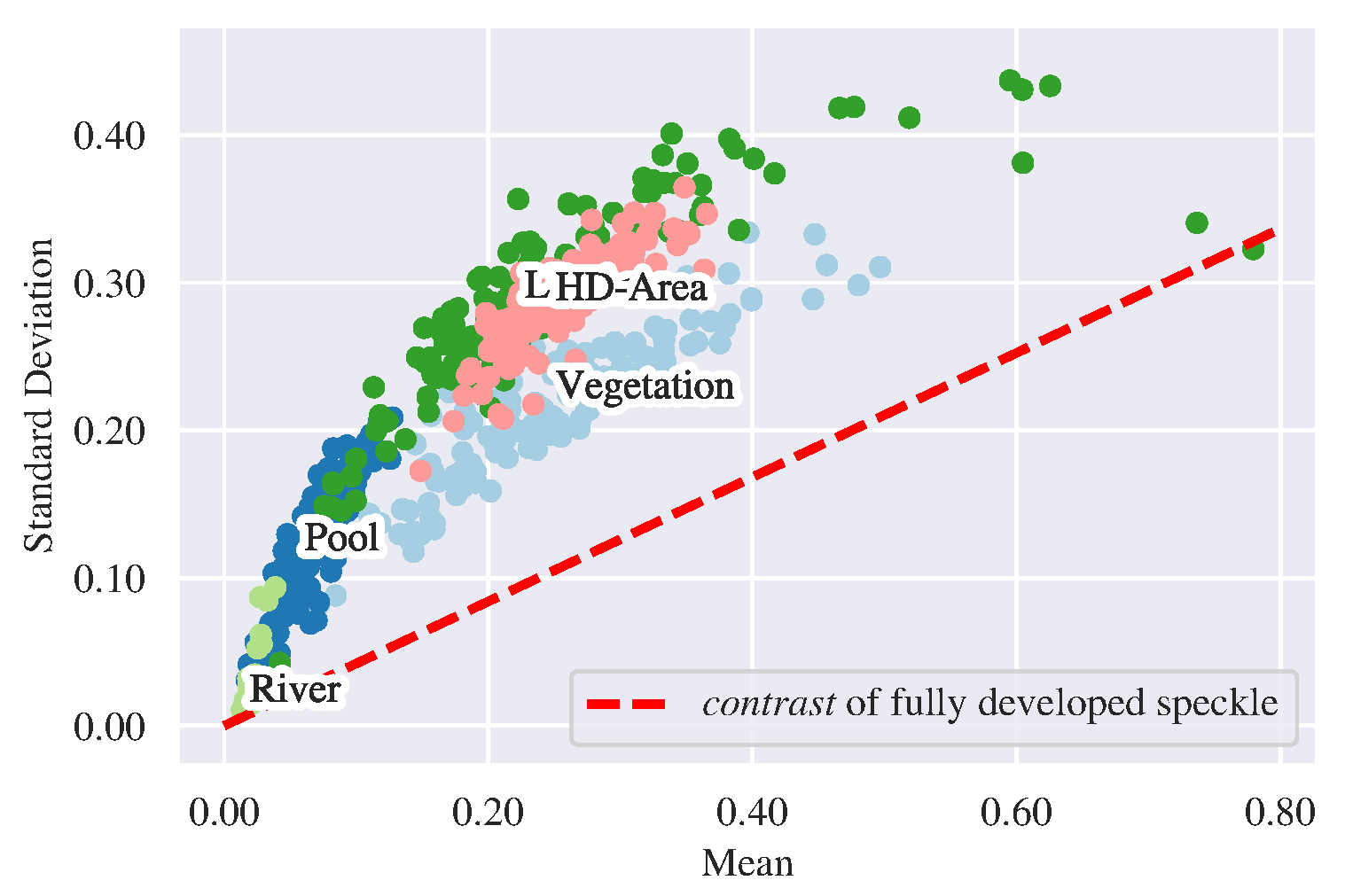
This paper bypasses the above estimation problem and lets and as the fluctuation representation for SAR image. In this context, the feature type is selected according to the specific domain knowledge about SAR data. When an SAR image is described by this fluctuation representation, the classification of this image can be performed straightforwardly based on this representation. However, the discrimination of this representation is often unsatisfactory. Figure 4 illustrates such an example. In Figure 4, the contrast of fully developed speckle is equal to , since the intensity of fully developed speckle follows a Gamma distribution with unit mean and variance. It can be observed that there are apparent inter-class confusions. In this paper, the mean and standard deviation of SAR images are used as primitives, and they are adaptively mapped into a high-dimensional feature space to fit more discriminative fluctuation representations by leveraging the power of neural networks.
3.2. Speckle Patterns Statistics Network
PSNet is composed of two sub-nets, including the discriminative net (DiscNet) and the pattern net (PatterNet), as shown in Figure 5. More specifically, in the DiscNet, the mean and standard deviation of the input are first extracted, and then they are adaptively mapped into a high-dimensional feature space to obtain the fluctuation representation for the input. In the PatterNet, the pattern representation of the input is extracted with hierarchical architecture. The contributions of the fluctuation representation and pattern representation to the final input representation are learned by minimizing the classification error.
3.2.1. DiscNet
The fluctuation representation is learned by DiscNet to describe the average fluctuation of SAR image. In the DiscNet, the mean and the standard deviation of the input are first extracted. Given an image , the mean and the standard deviation are given by
where denotes the ith pixel value, and n is the number of pixels. In order to extract with existing deep learning framework such as Caffe and Tensorflow [65,66], is re-expressed as
The extracted and are then automatically scaled and shifted by DiscNet to map them into a high-dimensional space , resulting in the feature vectors and . Taking for example, it can be mathematically expressed as
where and represent the scaling and shifting vectors, respectively. Finally, the interplays of and are optimized with respect to the classification error to form the fluctuation representation as follows:
where denotes the rectified linear unit activation function [67], and are the weight matrix and bias vector, respectively. Here, it is required that to ensure the fluctuation representation lies in a feature space with high dimensionality. This implementation is equivalent to the convolutional transformation with kernel size and M output channels. The intuition behind this implementation can be interpreted as: increasing the dimensionality of feature space with the expectation to improve the discrimination of the fluctuation representation.
3.2.2. PatterNet
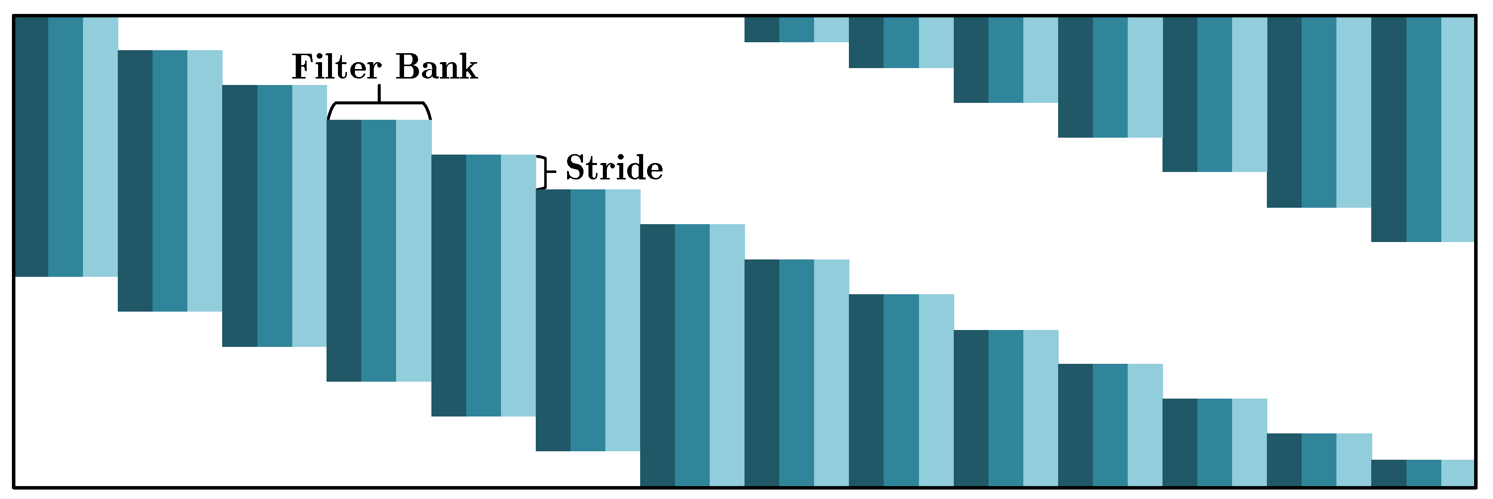
The pattern representation is extracted by PatterNet to hierarchically capture the spatial patterns lying in the input. PatterNet is a multi-layer model, including convolution, Pooling, ReLU and SPP layers [67]. The convolution layer performs spatial filtering to extract the texture feature, and this spatial filtering can be expressed as a matrix-vector multiplication [68]. Concretely, let and be the input and convolution matrix of the lth convolution layer, the spatial filtering can be expressed as . Note that has a sparse structure because of the weight sharing strategy [68], as illustrated in Figure 6. Subsequently, a series of transformations are performed, such as ReLU and Pooling. These transformations can be uniformly given by
where is the output of the lth layer, and is a composite function, such as ReLU or Pooling [67]. With this multi-layer model, the pattern representation is extracted by PatterNet for the input.
3.2.3. Optimization
The contributions of the fluctuation and pattern representations, and , to the final input representation are learned by minimizing the classification error. The final representation is expressed as
where and denote the weight matrices. The representation is fed into a softmax layer [67] for classification.
PSNet is an end-to-end learning model where the data representation and the classifier are learned together. More specifically, given a training set , where denote the label of training sample and N is the number of training samples, the learning procedure of PSNet can be mathematically formulated as the following optimization problem:
where denotes the predicted label of , and are the parameters to be learned in the lth layer of PSNet, and represents a loss function. In this paper, the cross-entropy [67] is used as the loss function measuring the divergence between two distributions, which is given by
where and denote the inner product [16] and the natural logarithm, respectively; is the label vector of the true label , generated by the One-Hot Encoding; represents the output of softmax layer [67]. Here, the jth output of softmax layer, , is defined by
where is the jth input of softmax layer and M is the number of input.
The above optimization problem can be effectively solved by the Stochastic Gradient Descent (SGD) algorithm [67]. In this paper, the gradients of loss function with respect to the parameters are estimated by every mini-batch of the training samples. Thus, the parameter in the lth layer is updated according to the following strategy:
where represents the gradient of loss function with respect to the parameter , and K is the number of training samples in a mini-batch, and is the learning rate. The gradient is calculated by the Back Propagation algorithm [67]. It should be noted that regularization [69] is used to avoid the overfitting problem during the training procedure.
4. Experiments
This section evaluates the performance of PSNet on real SAR data. The dataset and the experimental setting are given in Section 4.1 and Section 4.2, respectively. The experimental results are analyzed in Section 4.3.
4.1. Data Sets
Guangdong data: This data was acquired by the TerraSAR-X with StripMap model over an urban area of Guangdong province, China, in 2008. Figure 7 shows these data, which is a level 1B product with spatial enhanced and multi-looking ground range detected. These data were radiometrically calibrated and geometrically corrected with SNAP, a toolbox provided by the European Space Agency. The size of this data is 4656 × 7518 with 1.25 m pixel spacing both in the range and azimuth, and the looks in azimuth and range are 1.033 and 1.334, respectively. The ground truth image was generated by manual annotation according to the associated optical image which can be found in the Google Earth by the information (including longitude, latitude and acquisition date) provided in the metadata file. These data are mainly composed of five classes, including Vegetation, High-Density Residential Areas, Low-density Residential Areas, River, and Pool.
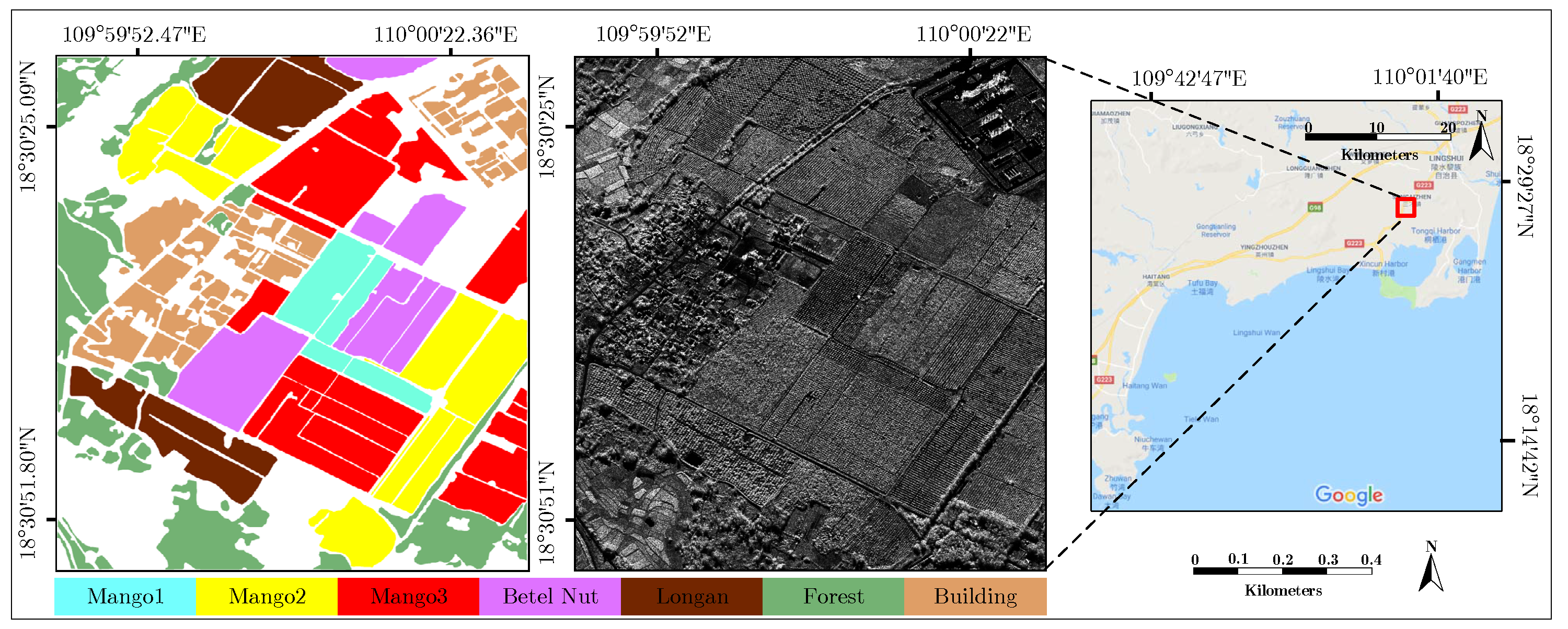
Orchard data: This data, displayed in Figure 8, was provided by the China Electronics Technology Group Corporation (CETC) 38th Institute [70]. It was acquired by the airborne sensor with X-band in Hainan province, China, in 2010. These data are a level 2 product, and the radiometric calibration and terrain correction were done by the provider. The size of these data is 2200 × 2400 with 0.5 × 0.5 m spatial resolution and four looks. The ground truth image, the left one in Figure 8, was generated by manual annotation according to our practical survey. This data consists of seven classes, including Mango1, Mango2, Mango3, Betel Nut, Longan, Forest, and Building. The unidentifiable target is shown in white in the ground truth image.
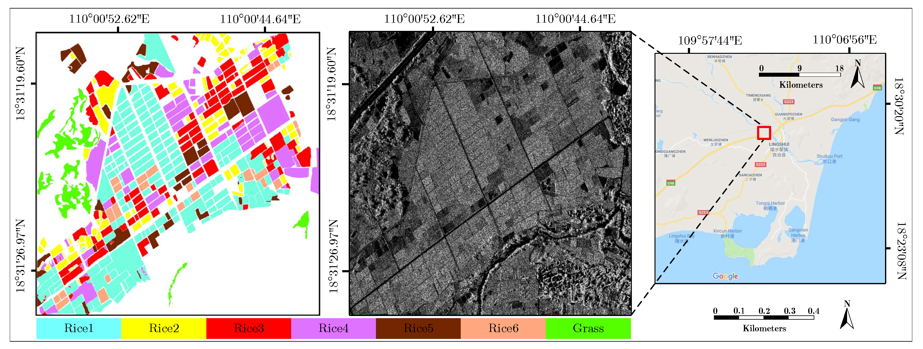
Rice data: It comes from an airborne sensor with an X-band over a cultivated area of Hainan in China in 2010. These data are a level 2 product, and it has 2048 × 2048 pixels with 0.5 × 0.5 m spatial resolution and four looks. Figure 9 shows these data; they are composed of seven categories where to represent the rice at different growth stages.
The training, validation and test sets are obtained as follows. Firstly, sub-images are randomly sampled from the original image according to the associated ground truth. Both non-overlapping and overlapping schemes are used to sample the sub-image. More specifically, for the Guangdong dataset, non-overlapping samples are drawn from the vegetation and river, while sub-images with an overlap of 14 pixels are sampled from other categories. As for the Orchard dataset and Rice dataset, an overlapping scheme (14 pixels) is used. Secondly, these sampled sub-images are shuffled and then m images per class, e.g., for the Orchard dataset, are randomly selected from these shuffled sub-images. Finally, these selected images are randomly divided into the training, validation and test sets which account for 60%, 15% and 25% of the total selected sub-images, respectively. Table 1 displays the details of Guangdong, Orchard and Rice datasets.
4.2. Experimental Settings
The CNN- and texture-based methods are considered for comparison, including standard CNN, spatial pyramid pooling network (SPPNet), GLCM, Gabor filtering and local binary pattern (LBP) [71]. The experimental settings are given as follows.
CNN: The structure of standard CNN is presented in Table 2. It consists of four convolution layers and two fully connected (FC) layers. This structure is used as the basic model in the experiment. Note that ReLU and Pooling layers are included in each convolution layer.
SPPNet: The architecture of SPPNet is similar to that of standard CNN except for the Pooling layer in Conv4. This Pooling layer is replaced by the SPP layer which performs max pooling with one level pyramid.
DiscNet: As displayed in Figure 5, both Conv1-1 and Conv2-1 have 64 output channels, and Conv3-1 has 128 channels. The output of Conv3-1 is fed into FC2 for classification. DiscNet is used to evaluate the effectiveness of the fluctuation representation.
PSNet: PSNet has two sub-nets: the DiscNet and the PatterNet, as shown in Figure 5. For the PatterNet, it shares the similar convolutional layers with the ones in standard CNN except Conv3 and Conv4. The Pooling layer in Conv3 is replaced by an SPP layer which performs max pooling with one level pyramid. The Conv4 is a convolution layer and the followed Pooling layer is removed. PSNet also has two FC layers and the settings remain consistent with that of standard CNN.
GLCM: Multiple GLCMs are created with two offsets, four orientations, (, , , ), and eight gray levels. The features considered for image description include contrast, correlation, energy, and inverse different moment.
Gabor: Gabor filters are implemented on four scales, (1, 3, 5, 7), and eight orientations, . The ratio of the mean and the standard deviation of each sub-band is used to describe the texture characteristics.
LBP: The input image is first divided into sub-patches, then the uniform LBP features are extracted from these sub-patches. These LBP features are concatenated to form the feature vector for the input image.
In the following experiments, the standard CNN, SPPNet, DiscNet, and PSNet are implemented with the Caffe deep learning framework [65]. Table 3 presents the training parameters. Note that the weight decay, namely, regularization, is used to prevent the overfitting. The classification in the GLCM, Gabor and LBP is performed by a nonlinear Support Vector Machine (SVM) [72]. The kernel type used in the SVM is the radial basis function, where the cost is tuned on the validation set and the gamma is set to default.
Evaluation metrics include the classification accuracy for each class, the average accuracy (AA), the overall accuracy (OA), and the Kappa coefficient (). AA is calculated by dividing the sum of accuracy of individual classes to the total number of classes. OA is the ratio of the number of correctly classified pixels to the total number of pixels. measures the proportion of agreement after chance agreements have been removed from considerations. It is defined as: , where is the accuracy of observed agreement, and is the estimate of chance agreement [73].
4.3. Results
4.3.1. Validation Accuracy
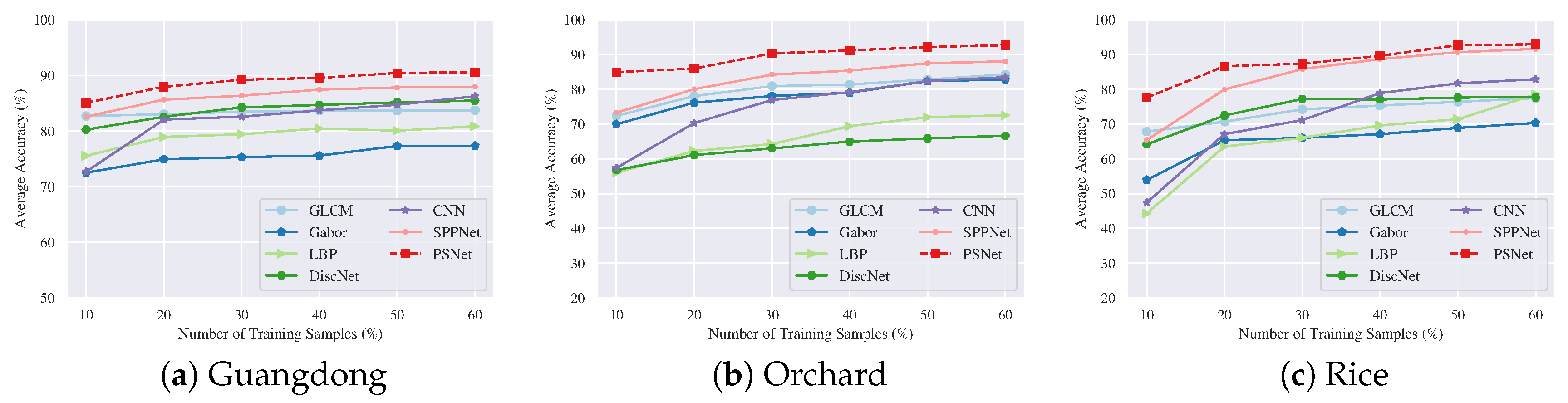
Figure 10 shows the average accuracy (AA) on the validation set with different numbers of training samples. Here, the validation set remains unchanged, while the samples used for training are randomly selected from the training set. The number of training samples, e.g., 10%, refers to the percentage of samples accounting for the total data in the dataset. The results in Figure 10 are obtained by 10 Monte Carlo runs.
From Figure 10, it can be observed that PSNet provides the highest AA than other methods even in the case of 10% training samples. This indicates that PSNet requires less training data. It is also interesting to note that DiscNet achieves promising performance, e.g., the results in Figure 10a,c. These results indicate that the fluctuation representation of SAR image is effective. However, DiscNet shows poor performance on the Orchard dataset, as displayed in Figure 10b. This is mainly because the images in the Orchard dataset present apparent structural features, as shown in Figure 11, whereas these features are not exploited by the DiscNet. For the GLCM, Gabor, and LBP, experimental results indicate that GLCM is better than Gabor and LBP. In the following experiments, GLCM is selected for comparison.
To verify the effectiveness of DiscNet, the following experiments are performed:
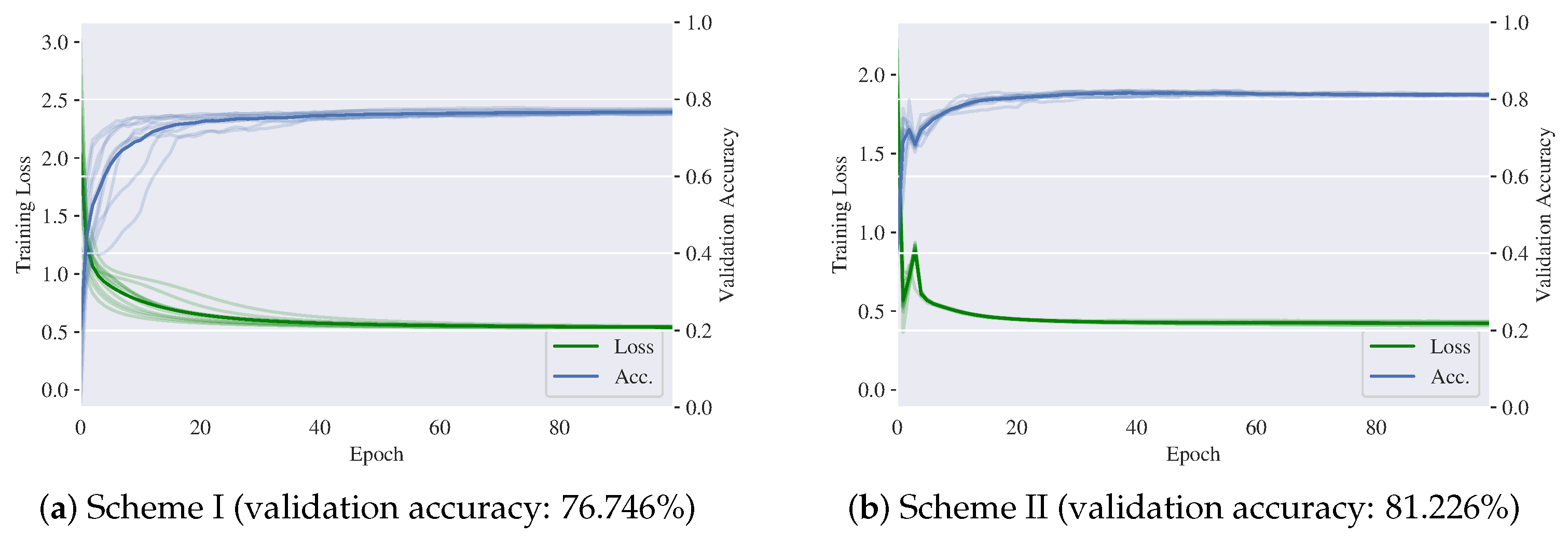
- Scheme I: the mean and standard deviation are directly used as the fluctuation representation;
- Scheme II: the fluctuation representation is fitted by the DiscNet.
Softmax classifier is used for Scheme I and Scheme II. Figure 12 and Figure 13 show the training loss and validation accuracy on the Guangdong dataset and the Orchard dataset, respectively. These results are obtained by 10 training runs. It can be observed that the validation accuracy benefits from the Scheme II, which demonstrates the effectiveness of DiscNet.
4.3.2. Classification Accuracy
The classification accuracy on the test set is investigated. In the following experiments, the samples used for training are 10% of the total samples in the Guangdong dataset and 30% both in the Orchard dataset and the Rice dataset.
Table 4 shows the results on the Guangdong dataset. It can be observed that PSNet achieves the highest AA of 85.04% and outperforms CNN and SPPNet in classifying the Vegetation, HD Area, and LD Area. The Vegetation and HD Area are typical mixed regions, resulting in high intra-class variations. For example, the HD Area consists of small-scale buildings, open land, streets, trees, and other classes. The higher classification accuracy benefits from the fluctuation representation extracted by the PSNet. This is also confirmed by the DiscNet, the classification accuracies of Vegetation and HD Area by DiscNet are up to 89.20% and 92.00%, respectively. For the LD Area, it is often composed of large-scale man-made buildings such as an industrial factory. Besides the structural feature, LD Area presents strong randomness. This is because: (1) the backscattering of LD Area is highly random and complex due to the existence of several phase centers; and (2) the spatial layouts of image elements in LD Area are generally random, since remote sensing images do not have an absolute reference. Therefore, it is crucial to describe the randomness of LD Area. In contrast to SPPNet and CNN, PSNet explicitly captures this randomness and therefore performs well in the LD Area.
Table 5 displays the results on Orchard dataset. The classification accuracy is improved by the PSNet, especially for Mango2, Longan, and Building. The AA of 90.29% achieved by PSNet is also higher than other methods. DiscNet performs effectively in classifying Mango1 with accuracy of 86.00%. However, the classification accuracy of Forest by DiscNet is only 20.00%. This is because the scattered echoes of Forest exhibit structural information, while DiscNet is not sensitive to the structural features.
Table 6 presents the results on the Rice dataset. It can be seen that PSNet performs better than other methods. The AA is significantly improved by PSNet, e.g., 13.92% and 3.92% respectively higher than CNN and SPPNet. In addition, Table 6 indicates that the classification of Rice3 and Rice4 is difficult. Compared with other methods, PSNet correctly classifies these two classes with high accuracy. The results in Table 6 demonstrate the effectiveness of PSNet.
4.3.3. Confusion Matrix
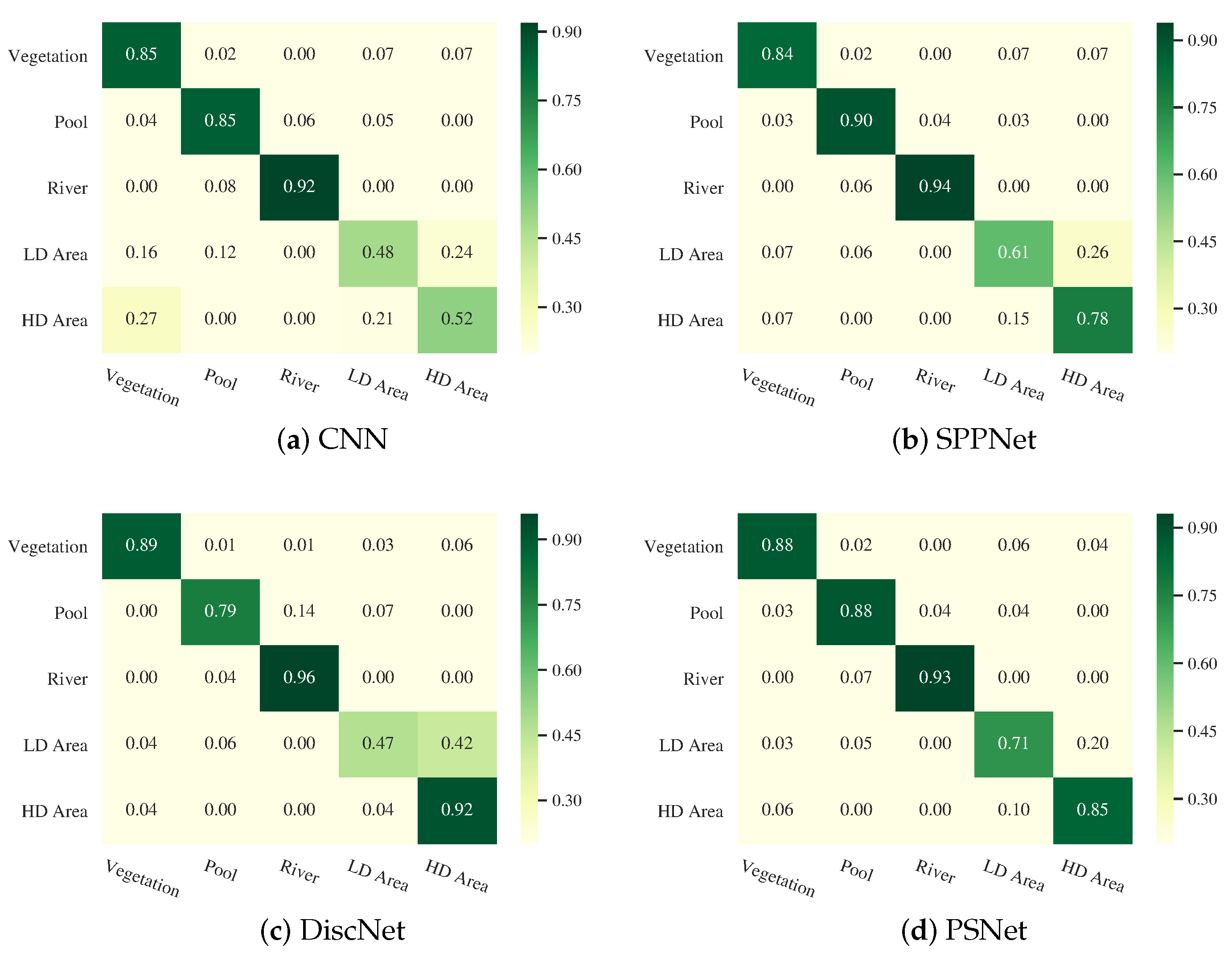
Figure 14 shows the confusion matrices for Guangdong dataset. It can be observed that the confusions mainly exist between the HD Area and the LD Area. For example, the misclassification probabilities of HD Area by CNN and PSNet are over 15.00%, as shown in Figure 14a,b. This confusion is reduced by the DiscNet, and the misclassification probability of HD Area drops to 4.00%. However, DiscNet misclassifies the LD Area as the HD Area with high risk. Compared with CNN and SPPNet, PSNet provides better performance in distinguishing the HD Area from the LD Area.
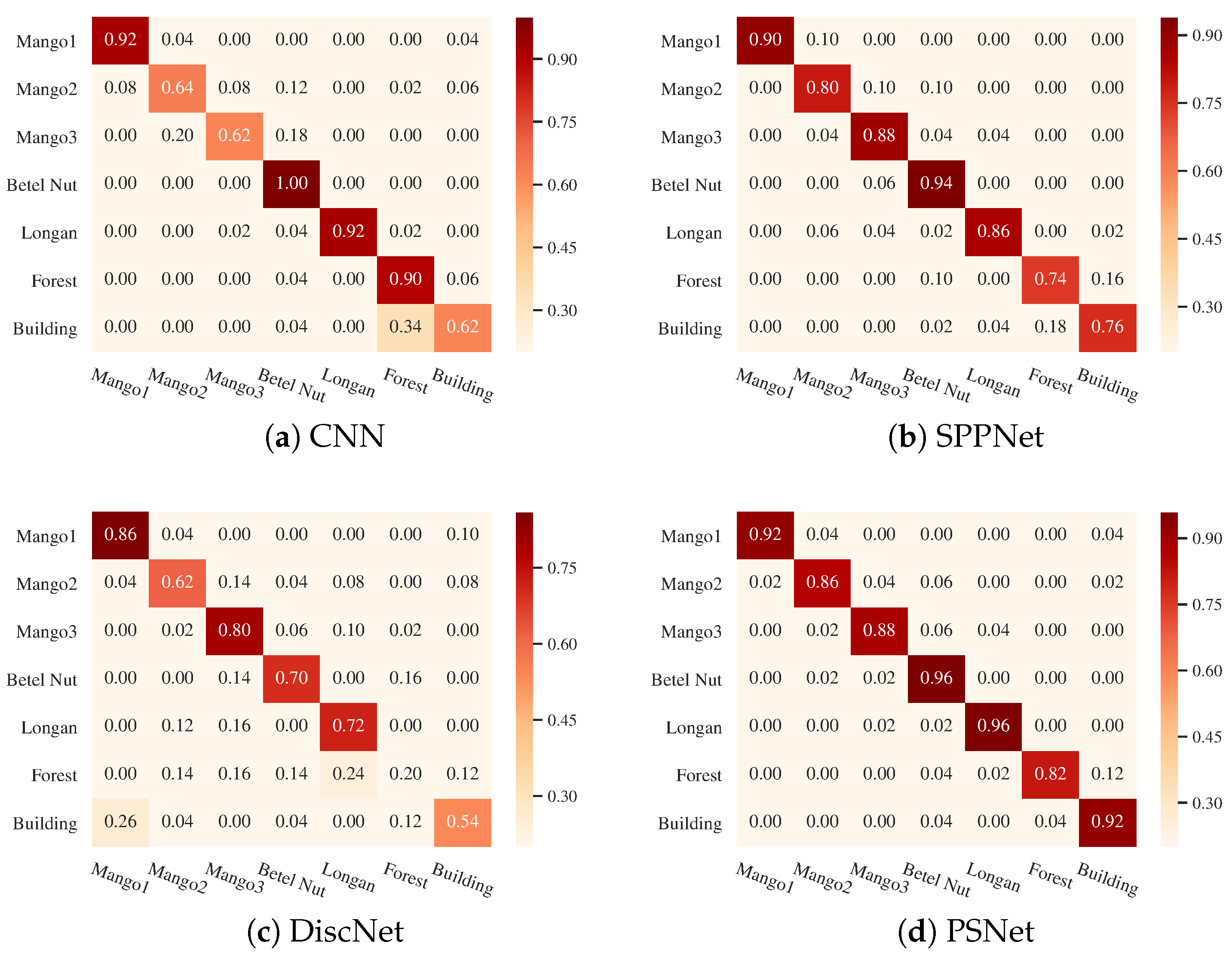
Figure 15 displays the results on Orchard dataset. It can be observed that Mango2 is difficult to be correctly recognized. For example, Mango2 is misclassified as Betel Nut by CNN and SPPNet with probabilities of 12.00% and 10.00%, respectively. This misclassification is significantly reduced to 6.00% by the PSNet, as shown in Figure 15d. The discriminative capability of DiscNet is unsatisfactory, especially for the Forest and the Building. This is because the structural feature is not extracted by the DiscNet.
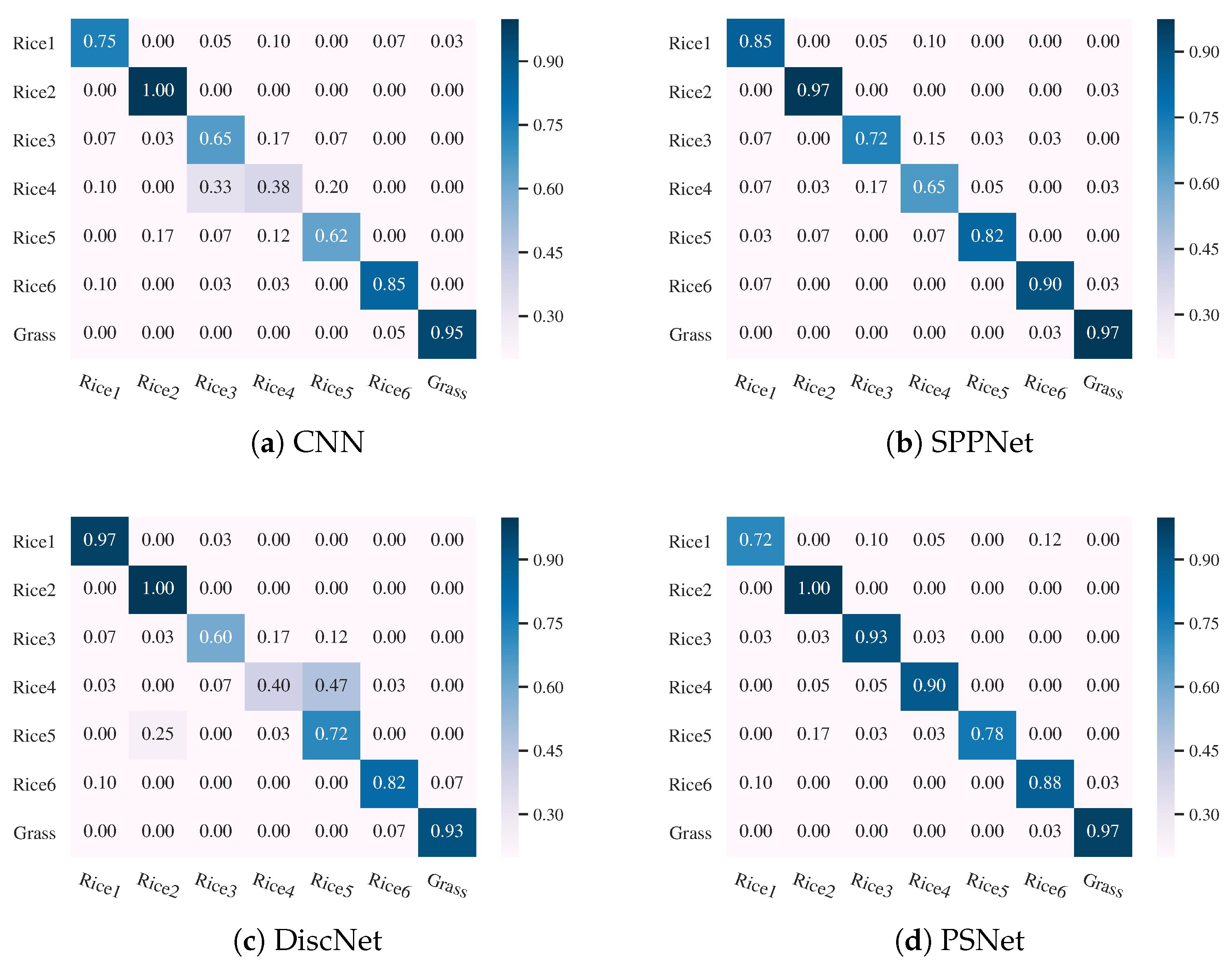
Figure 16 presents the confusion matrices for Rice dataset. It is apparent that there are confusions among Rice3, Rice4, and Rice5, as shown in Figure 16a,c. These confusions are reduced by the SPPNet, but there are still obvious confusions between Rice4 and Rice3. The confusions are further eliminated by the PSNet, as displayed in Figure 16d. The probability of misclassifying Rice3 as Rice4 drops to 3.00%. However, PSNet shows performance loss in recognizing Rice1.
4.3.4. Classification Map
The classification maps of Guangdong and Orchard data are qualitatively compared. To obtain the classification map, the sub-images, which are selected by a sliding window from the original image, are first classified to get the initial result. Then, this initial result is smoothed with a post-processing approach based on the conditional random fields [74] to generate the classification map. The strides of the sliding window in row and column directions for the Guangdong and Orchard data are set to 12 pixels and eight pixels, respectively.
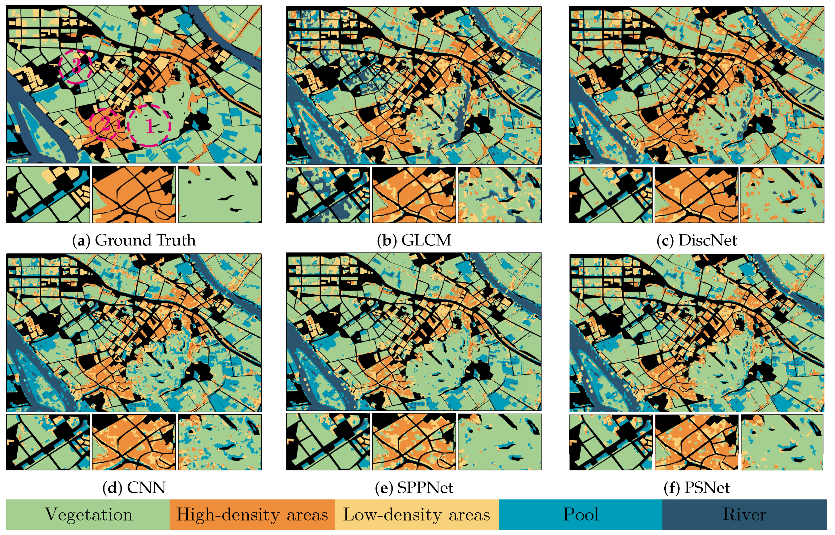
Figure 17 displays the results of Guangdong data. Three regions are highlighted in Figure 17a for the convenience of comparison. In the highlighted region 1, SPPNet and PSNet provide better performance than GLCM, DiscNet and CNN, as shown in Figure 17e,f. In region 2, PSNet performed well, while SPPNet misclassified a large portion of HD Area as the LD Area. It is interesting to note that DiscNet shows superior performance in region 2, which indicates that the fluctuation representation is useful. In region 3, the results achieved by DiscNet, CNN, SPPNet and PSNet were comparable, while the results by GLCM were unsatisfactory. Table 7 shows the qualitative comparison of each method. PSNet achieves the highest OA of 82.64% and AA of 72.37% with a of 0.75.
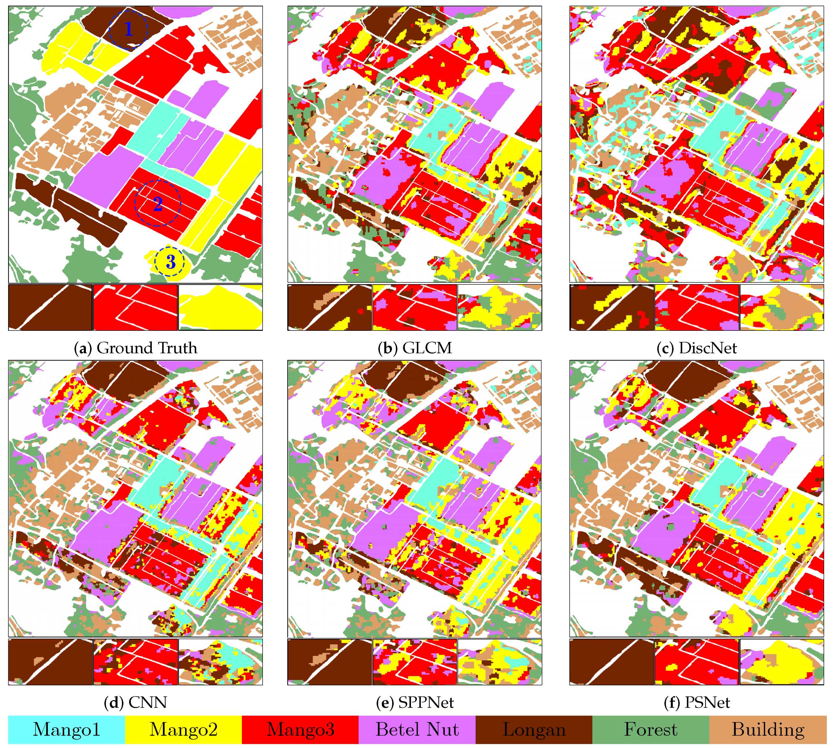
Figure 18 shows the results of Orchard data. In the highlighted region 1, PSNet obtains the best results. Almost all the Longans are correctly recognized by PSNet. In region 2, the classification of Mango3 is rather difficult and there apparent misclassification exists. Nevertheless, PSNet and GLCM perform comparably well. In region 3, most of the Mango2 are correctly classified by PSNet, while other methods provide poor classification performance. Table 8 shows the qualitative comparison of each method. PSNet provides the highest OA of 78.77% and AA of 72.47% with a of 0.74.
It should be pointed out that this paper mainly deals with the image-level classification problem. The above semantic segmentation results are only used for evaluation from the perspective of rapid scene understanding.
4.3.5. Feature Visualization
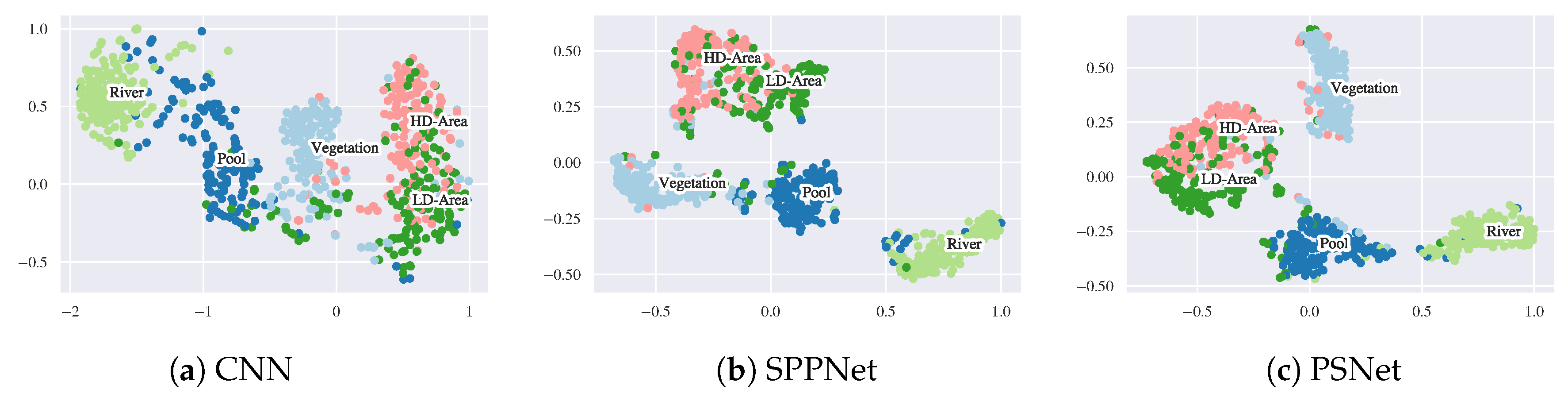
Figure 19 shows the feature visualization on the Guangdong dataset. Here, the high-dimensional features of the first fully connected layer are converted into 2D space by the T-distributed Stochastic Neighbor Embedding (t-SNE) [75] and the results are visualized. From Figure 19b, the results by CNN present large overlaps between each class, especially between the HD Area and the LD Area. These overlaps are reduced by the SPPNet and PSNet, as shown in Figure 19c,d. Moreover, compared with SPPNet, the clusters of HD Area and LD Area formed by PSNet are more distinctive, and therefore the separation between these classes becomes easy. These results indicate that the features extracted by the PSNet are more discriminative.
5. Discussion
The experimental results indicate that the proposed PSNet improves classification accuracy. For example, PSNet respectively outperforms the standard CNN and SPPNet in terms of average accuracy by 12.56% and 3.68% on the Guangdong dataset, by 10.00% and 5.29% on the Orchard dataset, and by 13.92% and 3.92% on the Rice dataset. Moreover, PSNet performs well in the case of high intra-class variations. For example, PSNet provides the highest classification accuracy for HD Area, Building and Rice3. A few discussions on this approach are given as follows.
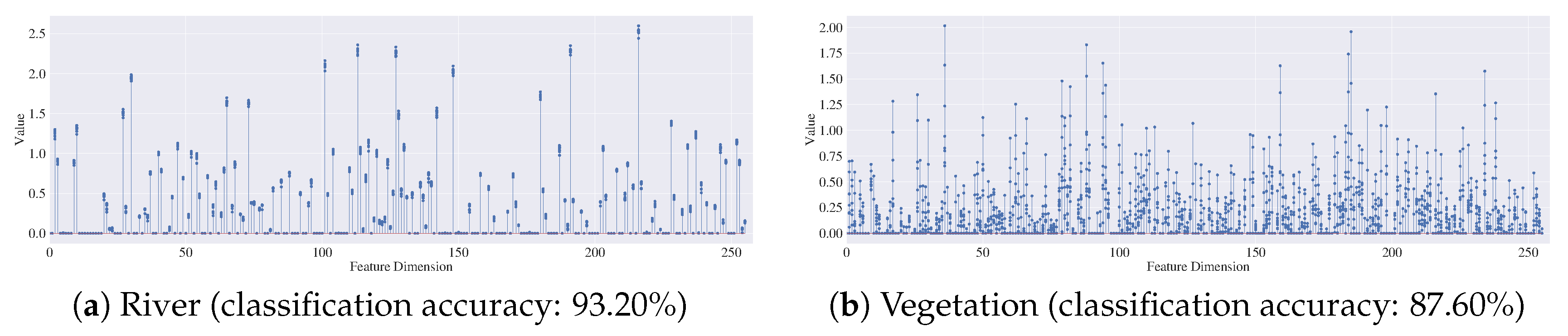
The sparsity of SAR image representation contributes to the classification accuracy. In [76], by placing sparsity constraints on an autoencoder, the discriminant of feature is enhanced, which contributes to the classification accuracy. For example, Figure 20 displays the features extracted by PSNet for the River and the Vegetation in the Guangdong dataset. It can be observed that the feature vector of River, with higher classification accuracy, tends to be sparser than that of Vegetation. This implies that it would be useful to enhance the feature discriminant by placing sparsity constraints. PSNet has not yet considered the sparsity constraint. Therefore, it would be helpful to further improve the feature discriminant.
In the proposed PSNet, the feature vector of SAR image comes from the interplays of its fluctuation and texture representations. The weight matrices, and in Equation (14), not only control the updating directions of and but also the contributions of and to the feature vector . The relationship between and will be the interest of future research.
Multi-scale representation has not yet been considered by PSNet. Multi-scale representation is a well-known concept in image processing. It originated from the scale-space theory [77], multiresolution analysis [78], and image pyramid [79]. Recently, this concept has gained attention in the field of representation learning [80,81,82]. Taking CNNs as an example, the feed-forward architecture implicitly forms a Markov chain of the successive representations for the input. This means that the representations in the current layer are only derived from its previously connected layer. As a consequence, only the features extracted by the last layer are used for image representation. However, it is believed that the features in different layers describe multiple aspects of the input image [57,82]. Therefore, the multi-scale representation will be investigated in future work.
The effectiveness of the PSNet is evaluated on relatively small-scale data sets. SAR data often present strong variations because of the sensitivity to the imaging conditions, such as the incidence angle and the descent or ascent orbit. Therefore, the generalization capability of the proposed PSNet will be assessed on the large-scale dataset. In addition, since data augmentation is a common scheme used in the case of finite training samples, it would be interesting to enhance the robustness of PSNet to the speckle noise by data augmentation.
6. Conclusions
This paper has presented a pattern statistics network (PSNet) for single-polarized SAR image classification. In the PSNet, the inherent randomness of SAR image is explicitly considered in the representation learning, and both fluctuation and pattern representations for the speckle patterns are learned. The fluctuation representation describes the average fluctuation of local pixels, while the pattern representation hierarchically captures the spatial interactions between local pixels. The interplays of the fluctuation representation and the pattern representation are learned by minimizing the classification error to obtain the final description for SAR image. The experimental results on three real SAR data indicate that integrating the statistical mechanism of SAR image into the representation learning is useful, and the classification results by PSNet are more accurate. It is also observed that the PSNet performs well in classifying the SAR images with high intra-class variations.
In future work, PSNet will be evaluated on the large-scale dataset and multi-scale representation will be considered. It would be interesting to exploit more statistical information about the SAR image in representation learning. In addition, it would be helpful to enhance the discrimination of data representation by imposing sparsity constraint on the representation.
Author Contributions
C.H. and X.L. conceived and designed the research. D.X. contributed to the experiments and the analysis of results. M.L. contributed to the discussion and suggestions for this research. X.L. drafted the manuscript, which was revised by all authors.
Funding
This research was funded by the National Key Research and Development Program of China (No. 2016YFC0803000), the National Natural Science Foundation of China (No. 61331016, No. 41371342), and the Hubei Innovation Group (No. 2018CFA006).
Acknowledgments
The authors would like to thank the anonymous reviewers, whose insightful suggestions and comments significantly strengthened this paper.
Conflicts of Interest
The authors declare no conflict of interest.
References
- Moreira, A.; Prats-Iraola, P.; Younis, M.; Krieger, G.; Hajnsek, I.; Papathanassiou, K.P. A tutorial on synthetic aperture radar. IEEE Geosci. Remote Sens. Mag. 2013, 1, 6–43. [Google Scholar] [CrossRef] [Green Version]
- Ouchi, K. Recent trend and advance of synthetic aperture radar with selected topics. Remote Sens. 2013, 5, 716–807. [Google Scholar] [CrossRef]
- Breit, H.; Fritz, T.; Balss, U.; Lachaise, M.; Niedermeier, A.; Vonavka, M. TerraSAR-X SAR processing and products. IEEE Trans. Geosci. Remote Sens. 2009, 48, 727–740. [Google Scholar] [CrossRef]
- Seguin, G.; Srivastava, S.; Auger, D. Evolution of the RADARSAT Program. IEEE Geosci. Remote Sens. Mag. 2014, 2, 56–58. [Google Scholar] [CrossRef]
- Aschbacher, J.; Milagro-Pérez, M.P. The European Earth monitoring (GMES) programme: Status and perspectives. Remote Sens. Environ. 2012, 120, 3–8. [Google Scholar] [CrossRef]
- Gu, X.; Tong, X. Overview of China Earth Observation Satellite Programs. IEEE Geosci. Remote Sens. Mag. 2015, 3, 113–129. [Google Scholar]
- Tison, C.; Nicolas, J.M.; Tupin, F.; Maître, H. A new statistical model for Markovian classification of urban areas in high-resolution SAR images. IEEE Trans. Geosci. Remote Sens. 2004, 42, 2046–2057. [Google Scholar] [CrossRef]
- Esch, T.; Schenk, A.; Ullmann, T.; Thiel, M.; Roth, A.; Dech, S. Characterization of land cover types in TerraSAR-X images by combined analysis of speckle statistics and intensity information. IEEE Trans. Geosci. Remote Sens. 2011, 49, 1911–1925. [Google Scholar] [CrossRef]
- Mahdianpari, M.; Salehi, B.; Mohammadimanesh, F.; Motagh, M. Random forest wetland classification using ALOS-2 L-band, RADARSAT-2 C-band, and TerraSAR-X imagery. ISPRS J. Photogramm. Remote Sens. 2017, 130, 13–31. [Google Scholar] [CrossRef]
- Yang, X.; Yang, W.; Song, H.; Huang, P. Polarimetric SAR Image Classification Using Geodesic Distances and Composite Kernels. IEEE J. Sel. Top. Appl. Earth Obs. Remote Sens. 2018, 11, 1606–1614. [Google Scholar] [CrossRef]
- LeCun, Y.; Bottou, L.; Bengio, Y.; Haffner, P. Gradient-based learning applied to document recognition. Proc. IEEE 1998, 86, 2278–2324. [Google Scholar] [CrossRef] [Green Version]
- Zhu, X.X.; Tuia, D.; Mou, L.; Xia, G.S.; Zhang, L.; Xu, F.; Fraundorfer, F. Deep learning in remote sensing: A comprehensive review and list of resources. IEEE Geosci. Remote Sens. Mag. 2017, 5, 8–36. [Google Scholar] [CrossRef]
- Cheng, G.; Han, J.; Lu, X. Remote Sensing Image Scene Classification: Benchmark and State of the Art. Proc. IEEE 2017, 105, 1865–1883. [Google Scholar] [CrossRef]
- LeCun, Y.; Bengio, Y.; Hinton, G. Deep learning. Nature 2015, 521, 436–444. [Google Scholar] [CrossRef] [PubMed]
- Bengio, Y.; Courville, A.; Vincent, P. Representation learning: A review and new perspectives. IEEE Trans. Pattern Anal. Mach. Intell. 2013, 35, 1798–1828. [Google Scholar] [CrossRef] [PubMed]
- Xian-Da, Z. Matrix Analysis and Applications; Cambridge University Press: Cambridge, UK, 2017; pp. 27–36. [Google Scholar]
- Xian-Da, Z. Modern Signal Processing; Tsinghua University Press: Beijing, China, 2002; pp. 163–168. [Google Scholar]
- Tomiyasu, K. Tutorial review of synthetic-aperture radar (SAR) with applications to imaging of the ocean surface. Proc. IEEE 1978, 66, 563–583. [Google Scholar] [CrossRef]
- Shwartz-Ziv, R.; Tishby, N. Opening the black box of deep neural networks via information. arXiv 2017, arXiv:1703.00810. [Google Scholar]
- Zhang, L.; Ji, Q. Image segmentation with a unified graphical model. IEEE Trans. Pattern Anal. Mach. Intell. 2010, 32, 1406–1425. [Google Scholar] [CrossRef]
- Goodman, J.W. Some fundamental properties of speckle. JOSA 1976, 66, 1145–1150. [Google Scholar] [CrossRef]
- Motoyoshi, I.; Nishida, S.; Sharan, L.; Adelson, E.H. Image statistics and the perception of surface qualities. Nature 2007, 447, 206. [Google Scholar] [CrossRef]
- Shanmugan, K.S.; Narayanan, V.; Frost, V.S.; Stiles, J.A.; Holtzman, J.C. Textural features for radar image analysis. IEEE Trans. Geosci. Remote Sens. 1981, 3, 153–156. [Google Scholar] [CrossRef]
- Ulaby, F.T.; Kouyate, F.; Brisco, B.; Williams, T.L. Textural information in SAR images. IEEE Trans. Geosci. Remote Sens. 1986, GE-24, 235–245. [Google Scholar] [CrossRef]
- Argenti, F.; Lapini, A.; Bianchi, T.; Alparone, L. A tutorial on speckle reduction in synthetic aperture radar images. IEEE Geosci. Remote Sens. Mag. 2013, 1, 6–35. [Google Scholar] [CrossRef]
- Lee, J.S.; Jurkevich, L.; Dewaele, P.; Wambacq, P.; Oosterlinck, A. Speckle filtering of synthetic aperture radar images: A review. Remote Sens. Rev. 1994, 8, 313–340. [Google Scholar] [CrossRef]
- Deng, X.; López-Martínez, C.; Chen, J.; Han, P. Statistical Modeling of Polarimetric SAR Data: A Survey and Challenges. Remote Sens. 2017, 9, 348. [Google Scholar] [CrossRef]
- Sekine, M.; Mao, Y. Weibull Radar Clutter; IEE Press: London, UK, 1990. [Google Scholar]
- Jao, J. Amplitude distribution of composite terrain radar clutter and the κ-distribution. IEEE Trans. Antennas Propag. 1984, 32, 1049–1062. [Google Scholar]
- Lampropoulos, G.; Drosopoulos, A.; Rey, N.; Anastassopoulos. High resolution radar clutter statistics. IEEE Trans. Aerosp. Electron. Syst. 1999, 35, 43–60. [Google Scholar]
- Nicolas, J.; Tupin, F. Gamma mixture modeled with “second kind statistics”: Application to SAR image processing. IEEE Int. Geosci. Remote Sens. Symp. 2002, 4, 2489–2491. [Google Scholar]
- Li, H.; Krylov, V.A.; Fan, P.Z.; Zerubia, J.; Emery, W.J. Unsupervised Learning of Generalized Gamma Mixture Model With Application in Statistical Modeling of High-Resolution SAR Images. IEEE Trans. Geosci. Remote Sens. 2016, 54, 2153–2170. [Google Scholar] [CrossRef]
- Hau, C.C. Handbook of Pattern Recognition and Computer Vision; World Scientific: Singapore, 2015. [Google Scholar]
- Haralick, R.M.; Shanmugam, K.; Dinstein, I. Textural Features for Image Classification. IEEE Trans. Syst. Man Cybern. 1973, smc-3, 610–621. [Google Scholar] [CrossRef]
- Thomas, E.; Thiel, M.; Schenk, A.; Roth, A.; Muller, A.; Dech, S. Delineation of urban footprints from TerraSAR-X data by analyzing speckle characteristics and intensity information. IEEE Trans. Geosci. Remote Sens. 2010, 48, 905–916. [Google Scholar]
- Zhu, S.C.; Guo, C.E.; Wang, Y.; Xu, Z. What are textons? Int. J. Comput. Vis. 2005, 62, 121–143. [Google Scholar] [CrossRef]
- Cui, S.; Schwarz, G.; Datcu, M. Remote sensing image classification: No features, no clustering. IEEE J. Sel. Top. Appl. Earth Obs. Remote Sens. 2015, 8, 5158–5170. [Google Scholar] [CrossRef]
- Lazebnik, S.; Schmid, C.; Ponce, J. Beyond bags of features: Spatial pyramid matching for recognizing natural scene categories. In Proceedings of the IEEE Computer Society Conference on Computer Vision and Pattern Recognition, New York, NY, USA, 17–22 June 2006; pp. 2169–2178. [Google Scholar]
- Cross, G.R.; Jain, A.K. Markov random field texture models. IEEE Trans. Pattern Anal. Mach. Intell. 1983, PAMI-5, 25–39. [Google Scholar] [CrossRef]
- Moser, G.; Serpico, S.B.; Benediktsson, J.A. Land-cover mapping by Markov modeling of spatial–contextual information in very-high-resolution remote sensing images. Proc. IEEE 2013, 101, 631–651. [Google Scholar] [CrossRef]
- Fjortoft, R.; Delignon, Y.; Pieczynski, W.; Sigelle, M.; Tupin, F. Unsupervised classification of radar images using hidden Markov chains and hidden Markov random fields. IEEE Trans. Geosci. Remote Sens. 2003, 41, 675–686. [Google Scholar] [CrossRef]
- Deng, H.; Clausi, D.A. Gaussian MRF rotation-invariant features for image classification. IEEE Trans. Pattern Anal. Mach. Intell. 2004, 26, 951–955. [Google Scholar] [CrossRef]
- Frankot, R.T.; Chellappa, R. Lognormal Random-Field Models and Their Applications to Radar Image Synthesis. IEEE Trans. Geosci. Remote Sens. 1987, GE-25, 195–207. [Google Scholar] [CrossRef]
- Randen, T.; Husoy, J.H. Filtering for texture classification: A comparative study. IEEE Trans. Pattern Anal. Mach. Intell. 1999, 21, 291–310. [Google Scholar] [CrossRef]
- Bovik, A.C.; Clark, M.; Geisler, W.S. Multichannel texture analysis using localized spatial filters. IEEE Trans. Pattern Anal. Mach. Intell. 1990, 12, 55–73. [Google Scholar] [CrossRef]
- De Grandi, G.D.; Lee, J.S.; Schuler, D.L. Target detection and texture segmentation in polarimetric SAR images using a wavelet frame: Theoretical aspects. IEEE Trans. Geosci. Remote Sens. 2007, 45, 3437–3453. [Google Scholar] [CrossRef]
- He, C.; Li, S.; Liao, Z.; Liao, M. Texture Classification of PolSAR Data Based on Sparse Coding of Wavelet Polarization Textons. IEEE Trans. Geosci. Remote Sens. 2013, 51, 4576–4590. [Google Scholar] [CrossRef]
- Deng, L.; Jaitly, N. Deep discriminative and generative models for speech pattern recognition. In Handbook of Pattern Recognition and Computer Vision; World Scientific: Singapore, 2016; pp. 27–52. [Google Scholar]
- Nie, S.; Zheng, M.; Ji, Q. The deep regression bayesian network and its applications: Probabilistic deep learning for computer vision. IEEE Signal Process. Mag. 2018, 35, 101–111. [Google Scholar] [CrossRef]
- Salakhutdinov, R.; Larochelle, H. Efficient learning of deep Boltzmann machines. In Proceedings of the International Conference on Artificial Intelligence and Statistics, Sardinia, Italy, 13–15 May 2010; pp. 693–700. [Google Scholar]
- Hinton, G.E.; Osindero, S.; Teh, Y.W. A fast learning algorithm for deep belief nets. Neural Comput. 2006, 18, 1527–1554. [Google Scholar] [CrossRef] [PubMed]
- Liu, F.; Jiao, L.; Hou, B.; Yang, S. POL-SAR image classification based on Wishart DBN and local spatial information. IEEE Trans. Geosci. Remote Sens. 2016, 54, 3292–3308. [Google Scholar] [CrossRef]
- Lv, Q.; Dou, Y.; Niu, X.; Xu, J.; Xu, J.; Xia, F. Urban land use and land cover classification using remotely sensed SAR data through deep belief networks. J. Sens. 2015, 2015, 538063. [Google Scholar] [CrossRef]
- Zhao, Z.; Jiao, L.; Zhao, J.; Gu, J.; Zhao, J. Discriminant deep belief network for high-resolution SAR image classification. Pattern Recognit. 2017, 61, 686–701. [Google Scholar] [CrossRef]
- Goodfellow, I.; Pouget-Abadie, J.; Mirza, M.; Xu, B.; Warde-Farley, D.; Ozair, S.; Courville, A.; Bengio, Y. Generative adversarial nets. In Proceedings of the Advances in Neural Information Processing Systems, Montreal, QC, Canada, 8–13 December 2014; pp. 2672–2680. [Google Scholar]
- He, K.; Zhang, X.; Ren, S.; Sun, J. Deep residual learning for image recognition. In Proceedings of the IEEE Conference on Computer Vision and Pattern Recognition, Las Vegas, NV, USA, 26 June–1 July 2016; pp. 770–778. [Google Scholar]
- Huang, G.; Liu, Z.; Van Der Maaten, L.; Weinberger, K.Q. Densely connected convolutional networks. In Proceedings of the IEEE Conference on Computer Vision and Pattern Recognition, Honolulu, HI, USA, 21–26 July 2017; pp. 4700–4708. [Google Scholar]
- He, K.; Zhang, X.; Ren, S.; Sun, J. Spatial pyramid pooling in deep convolutional networks for visual recognition. IEEE Trans. Pattern Anal. Mach. Intell. 2015, 37, 1904–1916. [Google Scholar] [CrossRef] [PubMed]
- Geng, J.; Wang, H.; Fan, J.; Ma, X. Deep supervised and contractive neural network for SAR image classification. IEEE Trans. Geosci. Remote Sens. 2017, 55, 2442–2459. [Google Scholar] [CrossRef]
- Geng, J.; Fan, J.; Wang, H.; Ma, X.; Li, B.; Chen, F. High-resolution SAR image classification via deep convolutional autoencoders. IEEE Geosci. Remote Sens. Lett. 2015, 12, 2351–2355. [Google Scholar] [CrossRef]
- Zhou, Y.; Wang, H.; Xu, F.; Jin, Y.Q. Polarimetric SAR Image Classification Using Deep Convolutional Neural Networks. IEEE Geosci. Remote Sens. Lett. 2016, 13, 1935–1939. [Google Scholar] [CrossRef]
- Zhang, Z.; Wang, H.; Xu, F.; Jin, Y.Q. Complex-valued convolutional neural network and its application in polarimetric SAR image classification. IEEE Trans. Geosci. Remote Sens. 2017, 55, 7177–7188. [Google Scholar] [CrossRef]
- Shang, R.; Wang, J.; Jiao, L.; Stolkin, R.; Hou, B.; Li, Y. SAR Targets Classification Based on Deep Memory Convolution Neural Networks and Transfer Parameters. IEEE J. Sel. Top. Appl. Earth Obs. Remote Sens. 2018, 11, 2834–2846. [Google Scholar] [CrossRef]
- Anfinsen, S.N.; Doulgeris, A.P.; Eltoft, T. Estimation of the equivalent number of looks in polarimetric synthetic aperture radar imagery. IEEE Trans. Geosci. Remote Sens. 2009, 47, 3795–3809. [Google Scholar] [CrossRef]
- Jia, Y.; Shelhamer, E.; Donahue, J.; Karayev, S.; Long, J.; Girshick, R.; Guadarrama, S.; Darrell, T. Caffe: Convolutional Architecture for Fast Feature Embedding. arXiv 2014, arXiv:1408.5093. [Google Scholar]
- Abadi, M.; Agarwal, A.; Barham, P.; Brevdo, E.; Chen, Z.; Citro, C.; Corrado, G.S.; Davis, A.; Dean, J.; Devin, M.; et al. Tensorflow: Large-scale machine learning on heterogeneous distributed systems. arXiv 2016, arXiv:1603.04467. [Google Scholar]
- Goodfellow, I.; Bengio, Y.; Courville, A.; Bengio, Y. Deep Learning; MIT Press: Cambridge, MA, USA, 2016. [Google Scholar]
- Papyan, V.; Romano, Y.; Elad, M. Convolutional neural networks analyzed via convolutional sparse coding. arXiv 2016, arXiv:1607.08194. [Google Scholar]
- Bottou, L.; Curtis, F.E.; Nocedal, J. Optimization methods for large-scale machine learning. SIAM Rev. 2018, 60, 223–311. [Google Scholar] [CrossRef]
- China Electronics Technology Group Corporation 38 Institute. Available online: http://www.cetc38.com.cn/ (accessed on 7 September 2018).
- Ojala, T.; Pietikainen, M.; Maenpaa, T. Multiresolution gray-scale and rotation invariant texture classification with local binary patterns. IEEE Trans. Pattern Anal. Mach. Intell. 2002, 24, 971–987. [Google Scholar] [CrossRef]
- Maulik, U.; Chakraborty, D. Remote Sensing Image Classification: A survey of support-vector-machine-based advanced techniques. IEEE Geosci. Remote Sens. Mag. 2017, 5, 33–52. [Google Scholar] [CrossRef]
- Congalton, R.G. A review of assessing the accuracy of classifications of remotely sensed data. Remote Sens. Environ. 1991, 37, 35–46. [Google Scholar] [CrossRef]
- Fulkerson, B.; Vedaldi, A.; Soatto, S. Class segmentation and object localization with superpixel neighborhoods. In Proceedings of the IEEE International Conference on Computer Vision, Kyoto, Japan, 29 September–2 October 2009; pp. 670–677. [Google Scholar]
- Maaten, L.v.d.; Hinton, G. Visualizing data using t-SNE. J. Mach. Learn. Res. 2008, 9, 2579–2605. [Google Scholar]
- Geng, J.; Wang, H.; Fan, J.; Ma, X. SAR image classification via deep recurrent encoding neural networks. EEE Trans. Geosci. Remote Sens. 2018, 56, 2255–2269. [Google Scholar] [CrossRef]
- Lindeberg, T. Scale-space theory: A basic tool for analyzing structures at different scales. J. Appl. Stat. 1994, 21, 225–270. [Google Scholar] [CrossRef]
- Mallat, S.G. A theory for multiresolution signal decomposition: the wavelet representation. IEEE Trans. Pattern Anal. Mach. Intell. 1989, 11, 674–693. [Google Scholar] [CrossRef] [Green Version]
- Burt, P.; Adelson, E. The Laplacian pyramid as a compact image code. IEEE Trans. Commun. 1983, 31, 532–540. [Google Scholar] [CrossRef]
- Huang, G.; Chen, D.; Li, T.; Wu, F.; van der Maaten, L.; Weinberger, K.Q. Multi-scale dense networks for resource efficient image classification. arXiv 2017, arXiv:1703.09844. [Google Scholar]
- Erhan, D.; Szegedy, C.; Toshev, A.; Anguelov, D. Scalable object detection using deep neural networks. In Proceedings of the IEEE Conference on Computer Vision and Pattern Recognition, Columbus, OH, USA, 23–28 June 2014; pp. 2147–2154. [Google Scholar]
- Yang, S.; Ramanan, D. Multi-scale recognition with DAG-CNNs. In Proceedings of the IEEE International Conference on Computer Vision, Santiago, Chile, 7–13 December 2015; pp. 1215–1223. [Google Scholar]
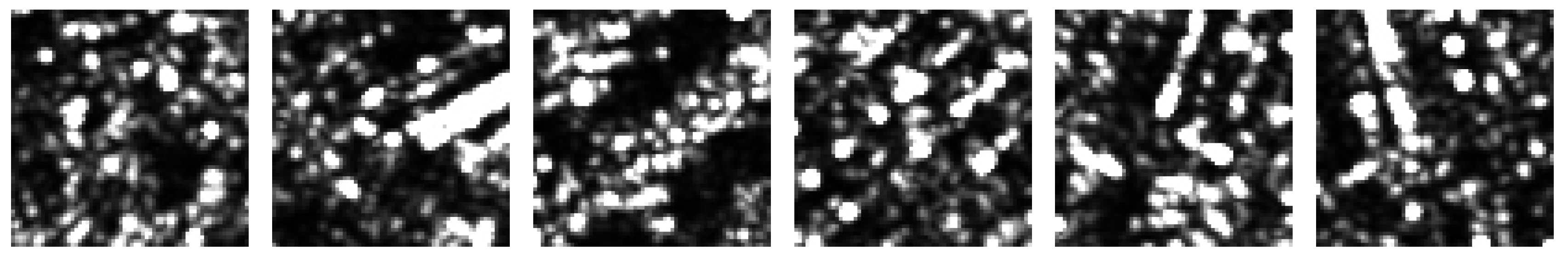
Figure 1.
High intra-class diversity of SAR images. These six images come from a high-density residential area. Although they share the same class, i.e., the high-density residential area, they present random and ever-changing spatial patterns.
Figure 1.
High intra-class diversity of SAR images. These six images come from a high-density residential area. Although they share the same class, i.e., the high-density residential area, they present random and ever-changing spatial patterns.

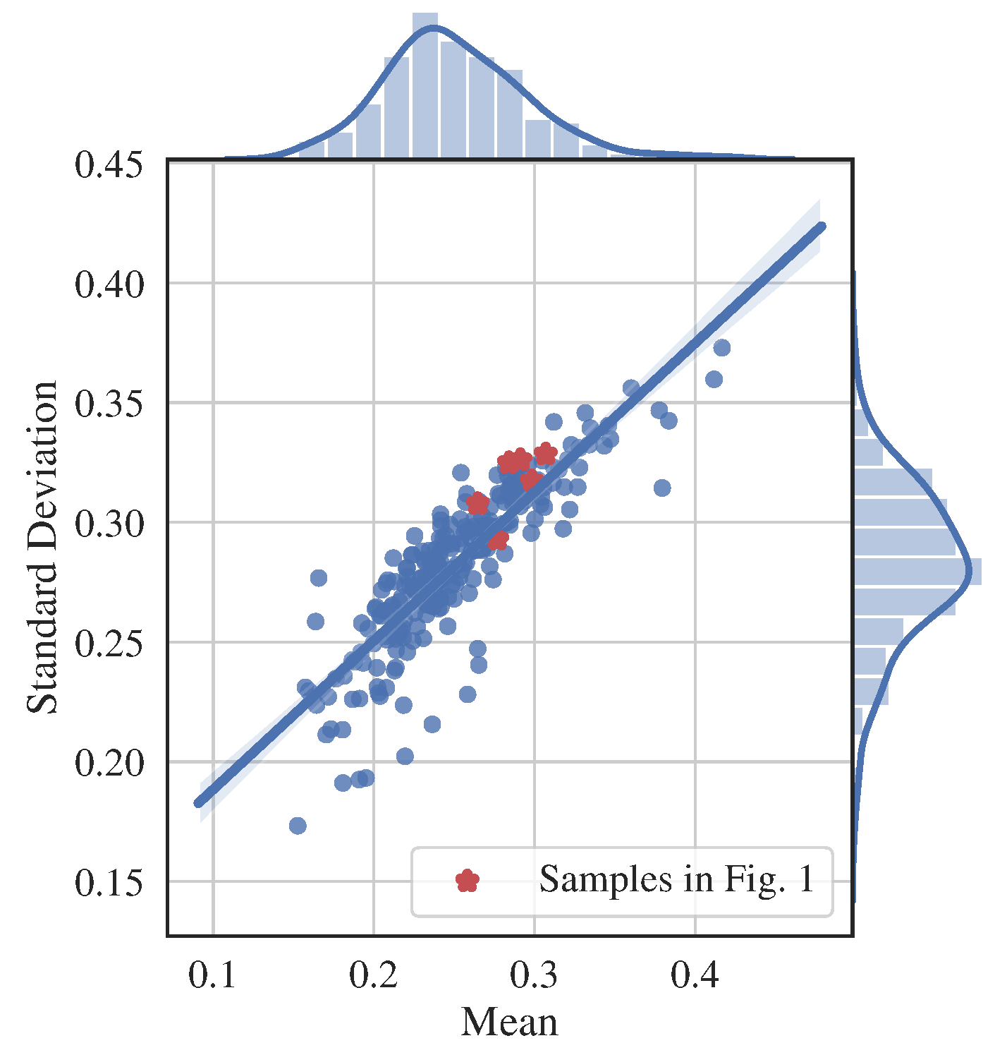
Figure 2.
SAR image representation with the mean and standard deviation. Here, the slope of the straight line is associated with the estimated coefficient of variation (see Equation (6)), which measures the local development of speckle patterns. The red points, corresponding to images in Figure 1, closely locate around the straight line. The high intra-class variations become non-salient.

Figure 3.
Framework of the proposed PSNet. The representation learned by the PSNet not only describes the average fluctuation of the input, but also captures the spatial pattern of the input.
Figure 3.
Framework of the proposed PSNet. The representation learned by the PSNet not only describes the average fluctuation of the input, but also captures the spatial pattern of the input.

Figure 4.
The discriminative capability of the mean and standard deviation. Five classes of TerraSAR-X images are represented by the mean and standard deviation which are estimated according to Equation (9). Although distinctive cluster centers are formed by River, Pool, and Vegetation, there are still apparent confusions between the high-density (HD) area and the low-density (LD) area.

Figure 5.
Architecture of the PSNet. PSNet consists of two sub-nets, including the DiscNet and the PatterNet, in which both fluctuation and pattern representations of SAR image are learned for the classification task. Max pooling is used in the PatterNet.
Figure 5.
Architecture of the PSNet. PSNet consists of two sub-nets, including the DiscNet and the PatterNet, in which both fluctuation and pattern representations of SAR image are learned for the classification task. Max pooling is used in the PatterNet.

Figure 6.
Convolution matrix with sparse structure. Here, the columns of the filter bank correspond to the filters used for spatial filtering, e.g., three filters in this example, and the stride is associated with the displacement in the convolution process. See more details in [68].
Figure 6.
Convolution matrix with sparse structure. Here, the columns of the filter bank correspond to the filters used for spatial filtering, e.g., three filters in this example, and the stride is associated with the displacement in the convolution process. See more details in [68].

Figure 7.
Overview of the Guangdong data. The unidentifiable class is shown in black in the ground truth image.
Figure 7.
Overview of the Guangdong data. The unidentifiable class is shown in black in the ground truth image.

Figure 8.
Overview of the Orchard data. The unidentifiable class is shown in white in a ground truth image.
Figure 8.
Overview of the Orchard data. The unidentifiable class is shown in white in a ground truth image.

Figure 9.
Overview of the Rice data. The unidentifiable class is shown in white in the ground truth image.
Figure 9.
Overview of the Rice data. The unidentifiable class is shown in white in the ground truth image.

Figure 10.
Average accuracy achieved on the validation set at different number of training samples. The proposed PSNet improves the average accuracy and it requires less training samples.
Figure 10.
Average accuracy achieved on the validation set at different number of training samples. The proposed PSNet improves the average accuracy and it requires less training samples.

Figure 11.
Representative examples with structural features in the Orchard dataset. (a) Mango2; (b) Mango3; (c) Longan; (d) Building.
Figure 11.
Representative examples with structural features in the Orchard dataset. (a) Mango2; (b) Mango3; (c) Longan; (d) Building.

Figure 12.
Training loss and validation accuracy of DiscNet on the Guangdong dataset (using 10% of data for training).
Figure 12.
Training loss and validation accuracy of DiscNet on the Guangdong dataset (using 10% of data for training).

Figure 13.
Training loss and validation accuracy of DiscNet on the Orchard dataset (using 30% of data for training).
Figure 13.
Training loss and validation accuracy of DiscNet on the Orchard dataset (using 30% of data for training).

Figure 14.
Confusion matrices for the Guangdong dataset.

Figure 15.
Confusion matrices for the Orchard dataset.

Figure 16.
Confusion matrices for the Rice dataset.

Figure 17.
Classification map overlaid with ground truth for the Guangdong data (using 10% of data for training). Three regions are highlighted in (a) for the convenience of comparison. The unidentifiable class is shown in black.
Figure 17.
Classification map overlaid with ground truth for the Guangdong data (using 10% of data for training). Three regions are highlighted in (a) for the convenience of comparison. The unidentifiable class is shown in black.

Figure 18.
Classification map overlaid with ground truth for the Orchard data (using 30% of data for training). Three regions are selected in (a) for the convenience of comparison. The unidentifiable class is shown in white.
Figure 18.
Classification map overlaid with ground truth for the Orchard data (using 30% of data for training). Three regions are selected in (a) for the convenience of comparison. The unidentifiable class is shown in white.

Figure 19.
Feature visualization on the Guangdong dataset. The high-dimensional features, extracted by the first fully connected layer, are mapped into 2D space by the t-SNE.
Figure 19.
Feature visualization on the Guangdong dataset. The high-dimensional features, extracted by the first fully connected layer, are mapped into 2D space by the t-SNE.

Figure 20.
Feature visualization. Here, ten samples are randomly selected from the River (a) and the Vegetation (b) in Guangdong dataset. The feature vectors extracted by PSNet for these samples are visualized.
Figure 20.
Feature visualization. Here, ten samples are randomly selected from the River (a) and the Vegetation (b) in Guangdong dataset. The feature vectors extracted by PSNet for these samples are visualized.


Table 1.
Details of the Guangdong, Orchard and Rice datasets.
| Dataset | #Class | #Samples per Class | Patch Size |
|---|---|---|---|
| Guangdong | 5 | 1000 | 64 × 64 pixels |
| Orchard | 7 | 200 | 64 × 64 pixels |
| Rice | 7 | 200 | 64 × 64 pixels |
Table 2.
Structure of the standard CNN deployed in the experiments.
| Conv1 | Conv2 | Conv3 | Conv4 | FC1 | FC2 |
|---|---|---|---|---|---|
| 3 × 3 kernel | 3 × 3 kernel | 3 × 3 kernel | 3 × 3 kernel | ||
| 1 stride | 1 stride | 1 stride | 1 stride | ||
| 12 channels | 32 channels | 64 channels | 128 channels | 256 channels | 7 channels |
| ReLU | ReLU | ReLU | ReLU | ReLU | |
| 2 × 2 pooling | 2 × 2 pooling | 2 × 2 pooling | 2 × 2 pooling |
Table 3.
Training parameters.
| Parameter | Value |
|---|---|
| base learning rate | 0.01 |
| learning rate policy | “inv” |
| gamma | 0.05 |
| power | 0.75 |
| momentum | 0.90 |
| weight decay | 0.001 |
| number of epochs | 100 |
Table 4.
Classification accuracy (%) on the Guangdong dataset. The bold number highlights the greatest classification accuracy per row.
Table 4.
Classification accuracy (%) on the Guangdong dataset. The bold number highlights the greatest classification accuracy per row.
| GLCM | DiscNet | CNN | SPPNet | PSNet | |
|---|---|---|---|---|---|
| Vegetation | 88.40 | 89.20 ± 0.01 | 84.80 ± 0.11 | 84.40 ± 0.04 | 87.60 ± 0.03 |
| Pool | 84.40 | 79.20 ± 0.01 | 85.20 ± 0.02 | 89.60 ± 0.01 | 88.40 ± 0.10 |
| River | 93.20 | 96.00 ± 0.00 | 92.00 ± 0.02 | 94.00 ± 0.01 | 93.20 ± 0.01 |
| LD Area | 63.20 | 47.20 ± 0.07 | 48.40 ± 0.06 | 60.80 ± 0.06 | 71.20 ± 0.16 |
| HD Area | 82.40 | 92.00 ± 0.09 | 52.00 ± 0.01 | 78.00 ± 0.04 | 84.80 ± 0.26 |
| AA | 82.32 | 80.72 ± 0.04 | 72.48 ± 0.04 | 81.36 ± 0.03 | 85.04 ± 0.11 |
Table 5.
Classification accuracy (%) on the Orchard dataset. The bold number highlights the greatest classification accuracy per row.
Table 5.
Classification accuracy (%) on the Orchard dataset. The bold number highlights the greatest classification accuracy per row.
| GLCM | DiscNet | CNN | SPPNet | PSNet | |
|---|---|---|---|---|---|
| Mango1 | 80.00 | 86.00 ± 0.02 | 92.00 ± 0.04 | 90.00 ± 0.13 | 92.00 ± 0.02 |
| Mango2 | 76.67 | 62.00 ± 0.17 | 64.00 ± 0.19 | 80.00 ± 0.21 | 86.00 ± 0.03 |
| Mango3 | 93.33 | 80.00 ± 0.10 | 62.00 ± 0.14 | 88.00 ± 0.14 | 88.00 ± 0.07 |
| Betel Nut | 93.33 | 70.00 ± 0.03 | 100.00 ± 0.07 | 94.00 ± 0.28 | 96.00 ± 0.05 |
| Longan | 73.33 | 72.00 ± 0.03 | 92.00 ± 0.07 | 86.00 ± 0.20 | 96.00 ± 0.03 |
| Forest | 76.67 | 20.00 ± 0.06 | 90.00 ± 0.20 | 74.00 ± 0.18 | 82.00 ± 0.15 |
| Building | 73.33 | 54.00 ± 0.01 | 62.00 ± 0.11 | 76.00 ± 0.16 | 92.00 ± 0.07 |
| AA | 80.95 | 63.43 ± 0.06 | 80.29 ± 0.12 | 84.00 ± 0.19 | 90.29 ± 0.06 |
Table 6.
Classification accuracy (%) on the Rice dataset. The bold number highlights the greatest classification accuracy per row.
Table 6.
Classification accuracy (%) on the Rice dataset. The bold number highlights the greatest classification accuracy per row.
| GLCM | DiscNet | CNN | SPPNet | PSNet | |
|---|---|---|---|---|---|
| Rice1 | 80.00 | 97.50 ± 0.01 | 75.00 ± 0.19 | 85.00 ± 0.31 | 72.50 ± 0.14 |
| Rice2 | 85.00 | 100.00 ± 0.00 | 100.00 ± 0.02 | 97.50 ± 0.02 | 100.00 ± 0.00 |
| Rice3 | 52.50 | 60.00 ± 0.13 | 65.00 ± 0.18 | 72.50 ± 0.25 | 92.50 ± 0.15 |
| Rice4 | 55.00 | 40.00 ± 0.02 | 37.50 ± 0.21 | 65.00 ± 0.16 | 90.00 ± 0.11 |
| Rice5 | 52.50 | 72.50 ± 0.05 | 62.50 ± 0.17 | 82.50 ± 0.17 | 77.50 ± 0.13 |
| Rice6 | 97.50 | 82.50 ± 0.04 | 85.00 ± 0.11 | 90.00 ± 0.31 | 87.50 ± 0.07 |
| Grass | 97.50 | 92.50 ± 0.03 | 95.00 ± 0.03 | 97.50 ± 0.04 | 97.50 ± 0.02 |
| AA | 74.29 | 77.86 ± 0.04 | 74.29 ± 0.13 | 84.29 ± 0.18 | 88.21 ± 0.09 |
Table 7.
Classification performance comparison on Guangdong data using overall accuracy (OA), average accuracy (AA) and Kappa coefficient ().
Table 7.
Classification performance comparison on Guangdong data using overall accuracy (OA), average accuracy (AA) and Kappa coefficient ().
| GLCM | DiscNet | CNN | SPPNet | PSNet | |
|---|---|---|---|---|---|
| OA | 73.93% | 76.69% | 74.93% | 81.35% | 82.65% |
| AA | 69.03% | 69.58% | 71.19% | 71.92% | 72.37% |
| 0.64 | 0.69 | 0.69 | 0.74 | 0.75 |
Table 8.
Classification performance comparison on Orchard data using overall accuracy (OA), average accuracy (AA) and Kappa coefficient ().
Table 8.
Classification performance comparison on Orchard data using overall accuracy (OA), average accuracy (AA) and Kappa coefficient ().
| GLCM | DiscNet | CNN | SPPNet | PSNet | |
|---|---|---|---|---|---|
| OA | 73.69% | 64.29% | 73.60% | 73.19% | 78.77% |
| AA | 69.01% | 53.64% | 66.23% | 64.77% | 72.47% |
| 0.68 | 0.56 | 0.68 | 0.67 | 0.74 |
© 2019 by the authors. Licensee MDPI, Basel, Switzerland. This article is an open access article distributed under the terms and conditions of the Creative Commons Attribution (CC BY) license (http://creativecommons.org/licenses/by/4.0/).
Share and Cite
MDPI and ACS Style
Liu, X.; He, C.; Xiong, D.; Liao, M. Pattern Statistics Network for Classification of High-Resolution SAR Images. Remote Sens. 2019, 11, 1942. https://0-doi-org.brum.beds.ac.uk/10.3390/rs11161942
AMA Style
Liu X, He C, Xiong D, Liao M. Pattern Statistics Network for Classification of High-Resolution SAR Images. Remote Sensing. 2019; 11(16):1942. https://0-doi-org.brum.beds.ac.uk/10.3390/rs11161942
Chicago/Turabian StyleLiu, Xinlong, Chu He, Dehui Xiong, and Mingsheng Liao. 2019. "Pattern Statistics Network for Classification of High-Resolution SAR Images" Remote Sensing 11, no. 16: 1942. https://0-doi-org.brum.beds.ac.uk/10.3390/rs11161942
Note that from the first issue of 2016, this journal uses article numbers instead of page numbers. See further details here.