Direct, ECOC, ND and END Frameworks—Which One Is the Best? An Empirical Study of Sentinel-2A MSIL1C Image Classification for Arid-Land Vegetation Mapping in the Ili River Delta, Kazakhstan

 ,
,  ,
,  , , , and
Abstract
:
1. Introduction
2. Materials and Methods
2.1. Materials
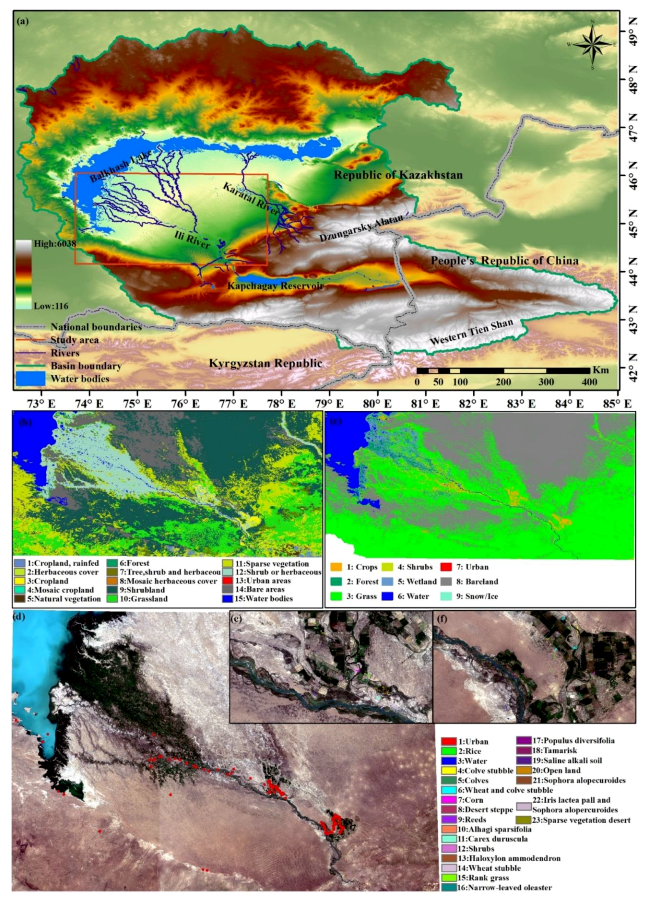
2.1.1. Study Region
2.1.2. Datasets
- Sentinel-2 data collection and preprocessing
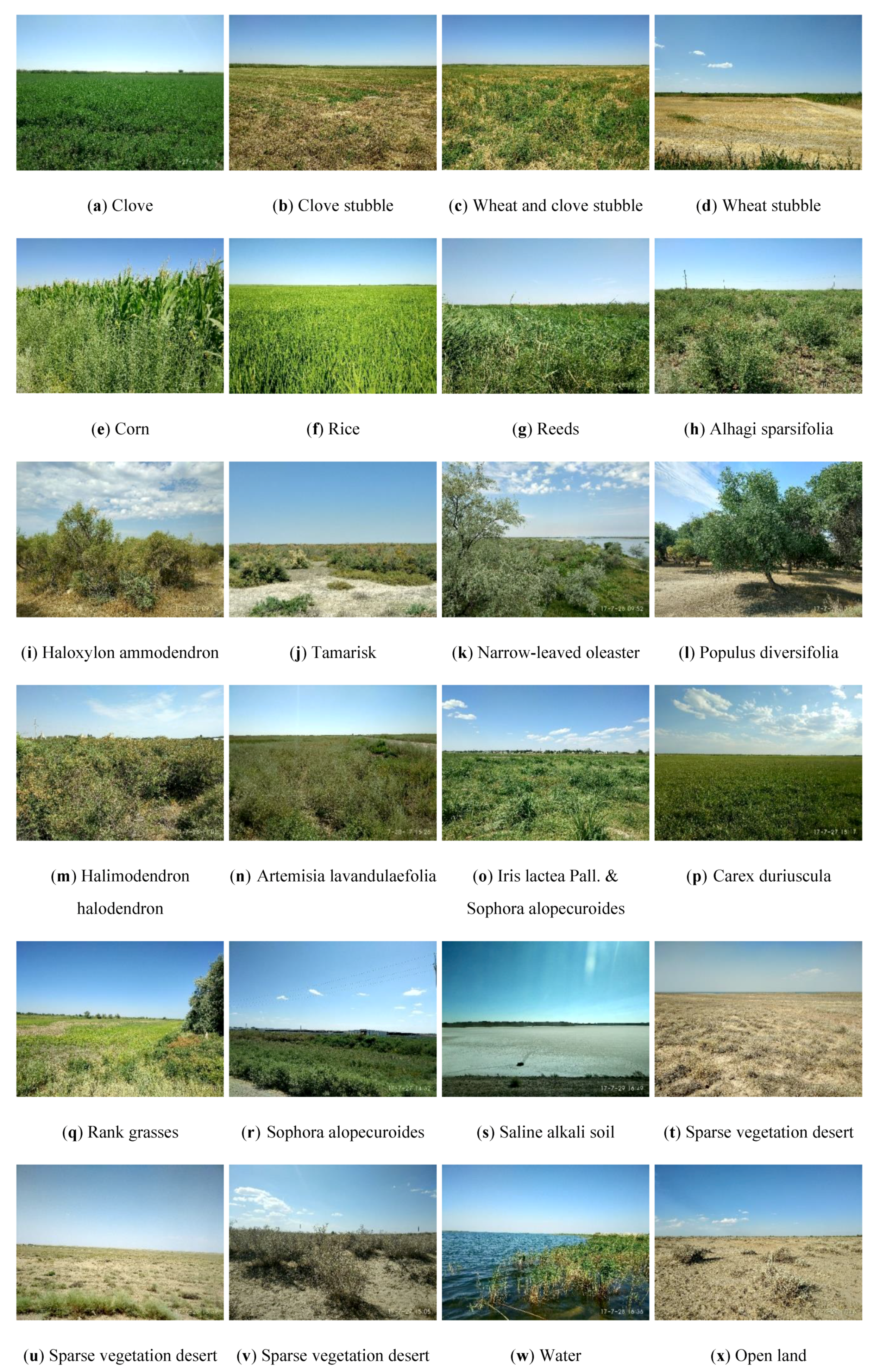
- In situ data collection
2.2. Methods
2.2.1. Related Methods
- Ensemble of nested dichotomies
- Multiresolution segmentation
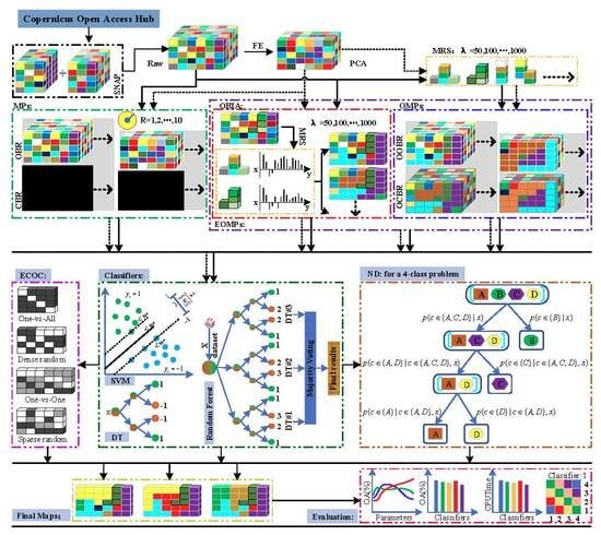
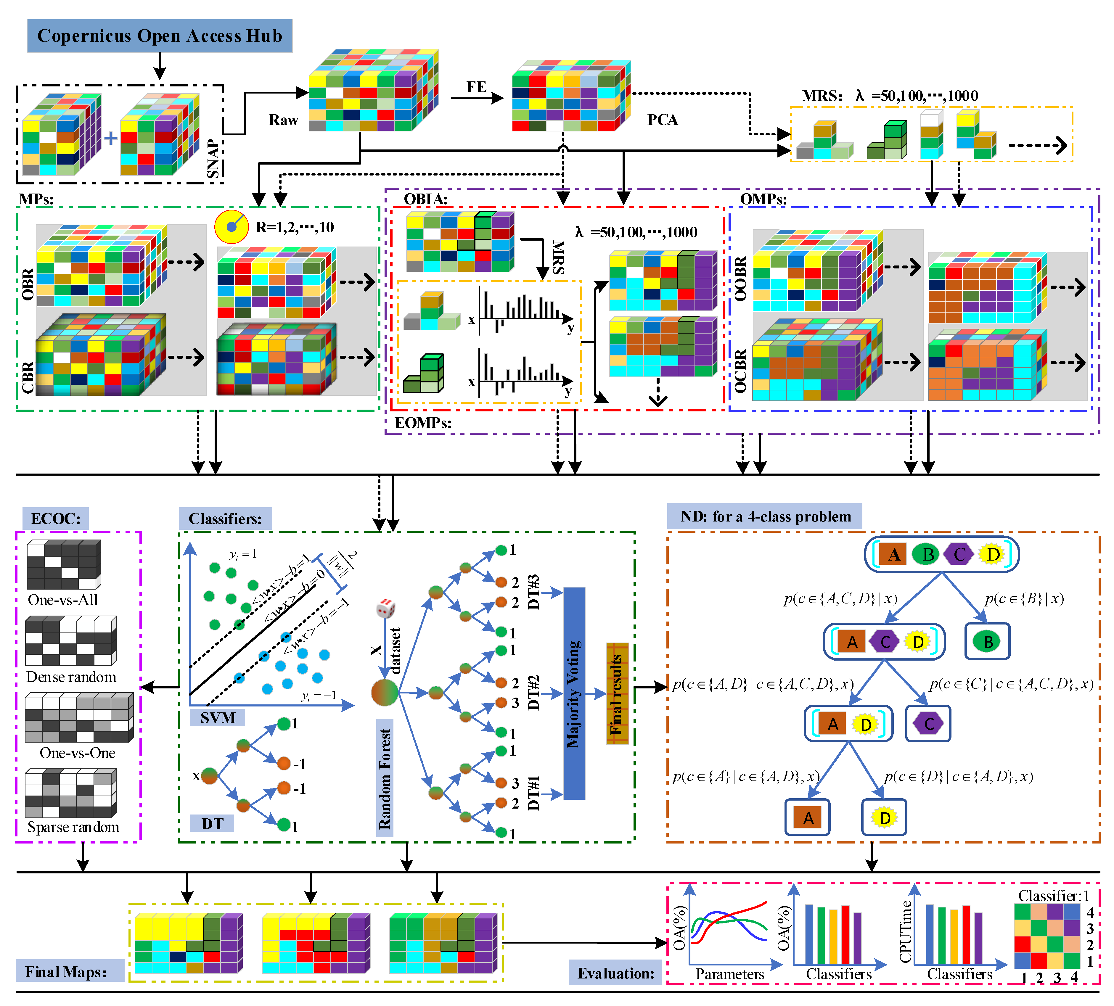
2.2.2. Proposed Method
2.2.3. Experimental Setup
3. Results
3.1. Subsection Assessment of the Feature Extractors
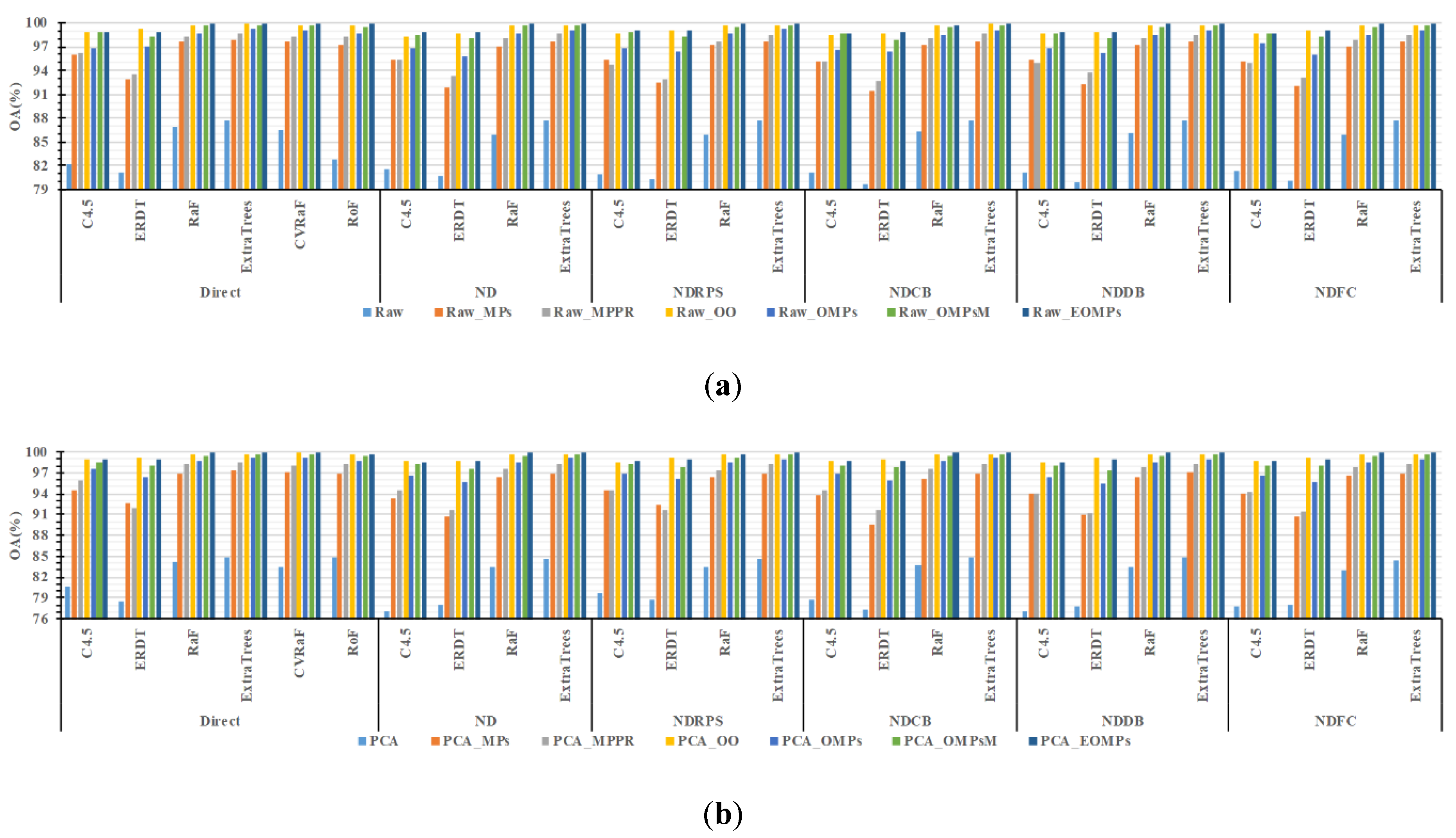
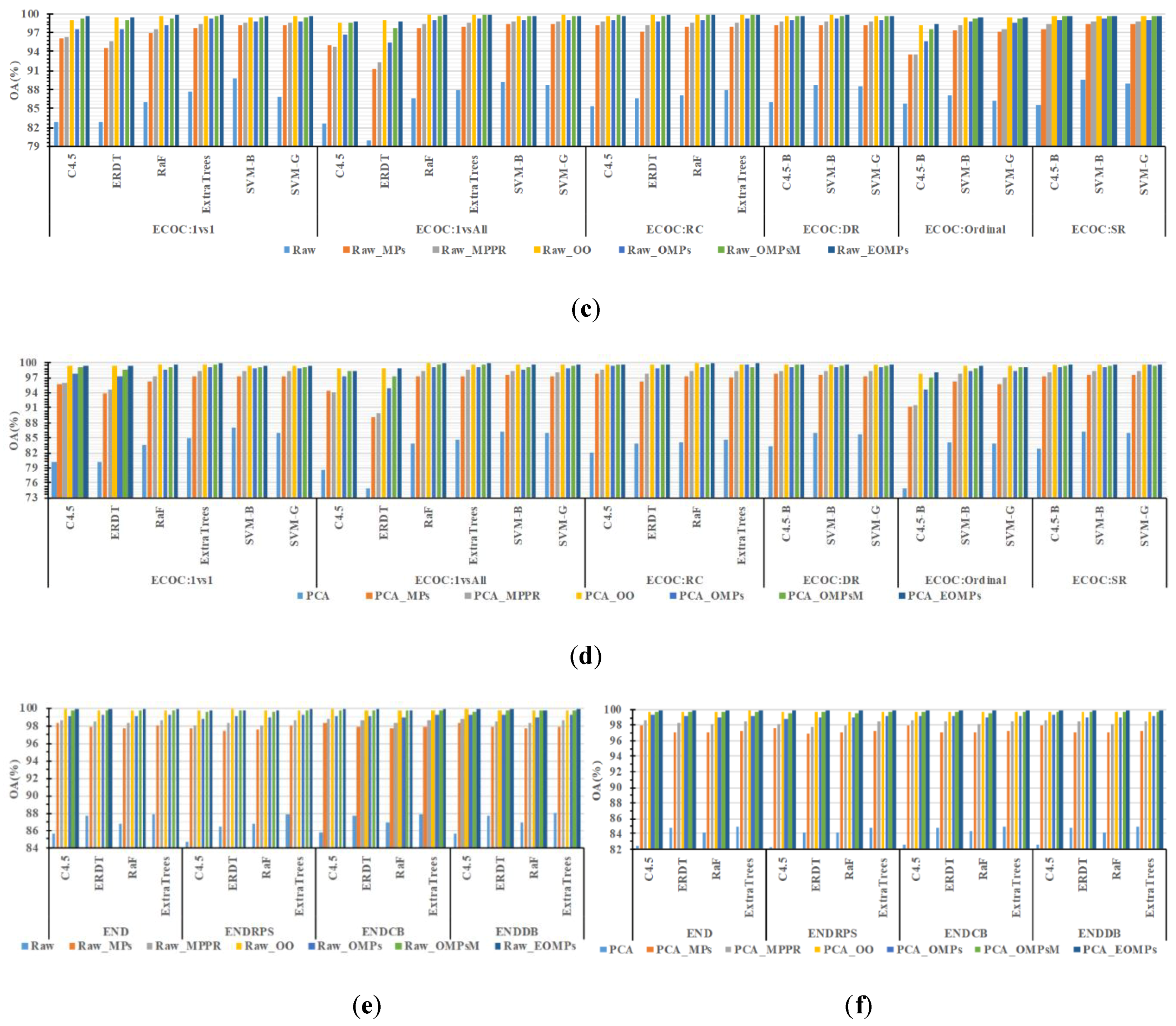
3.1.1. Accuracy Evaluation
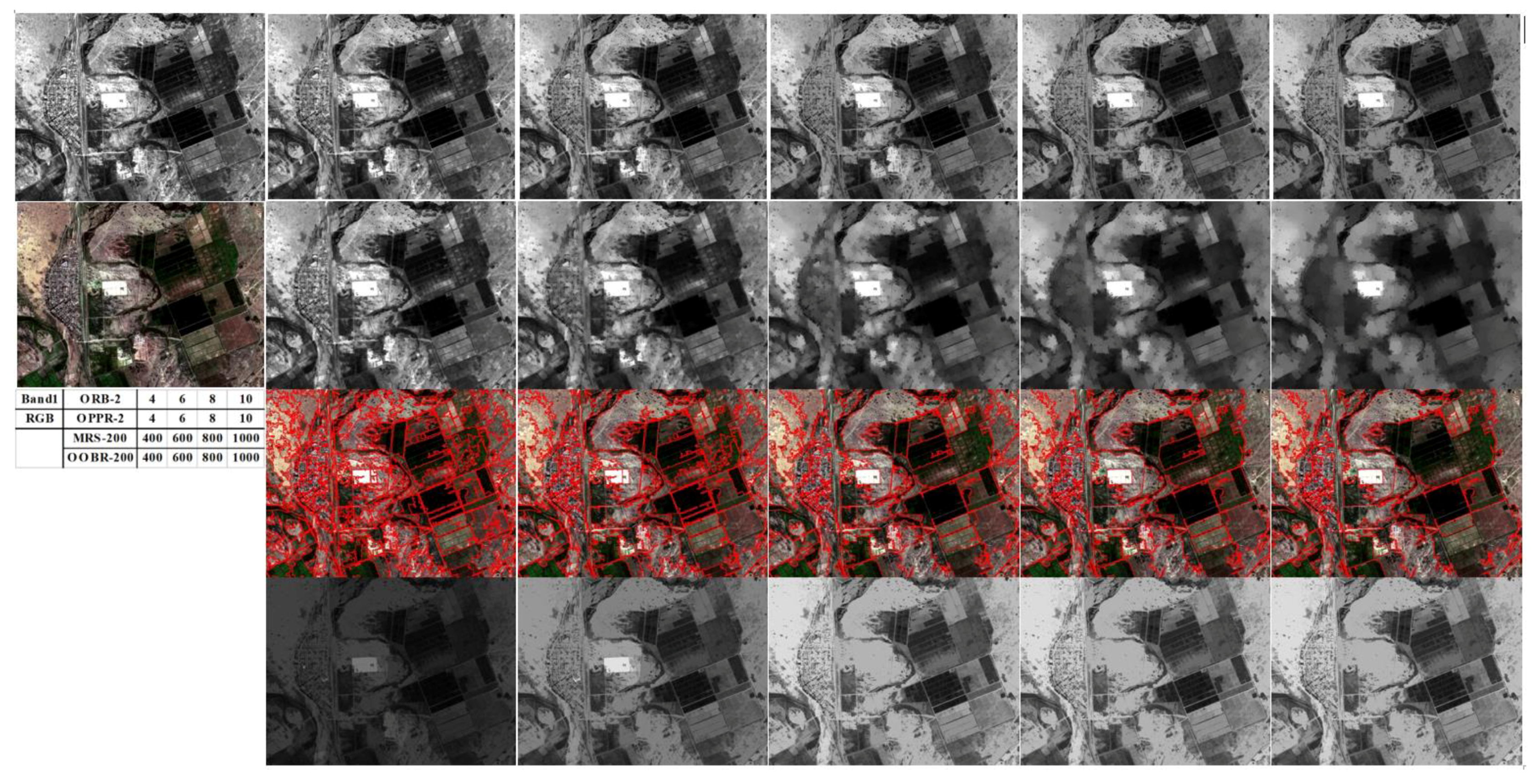
3.1.2. Visual Evaluation
3.2. Evaluation of ND and END
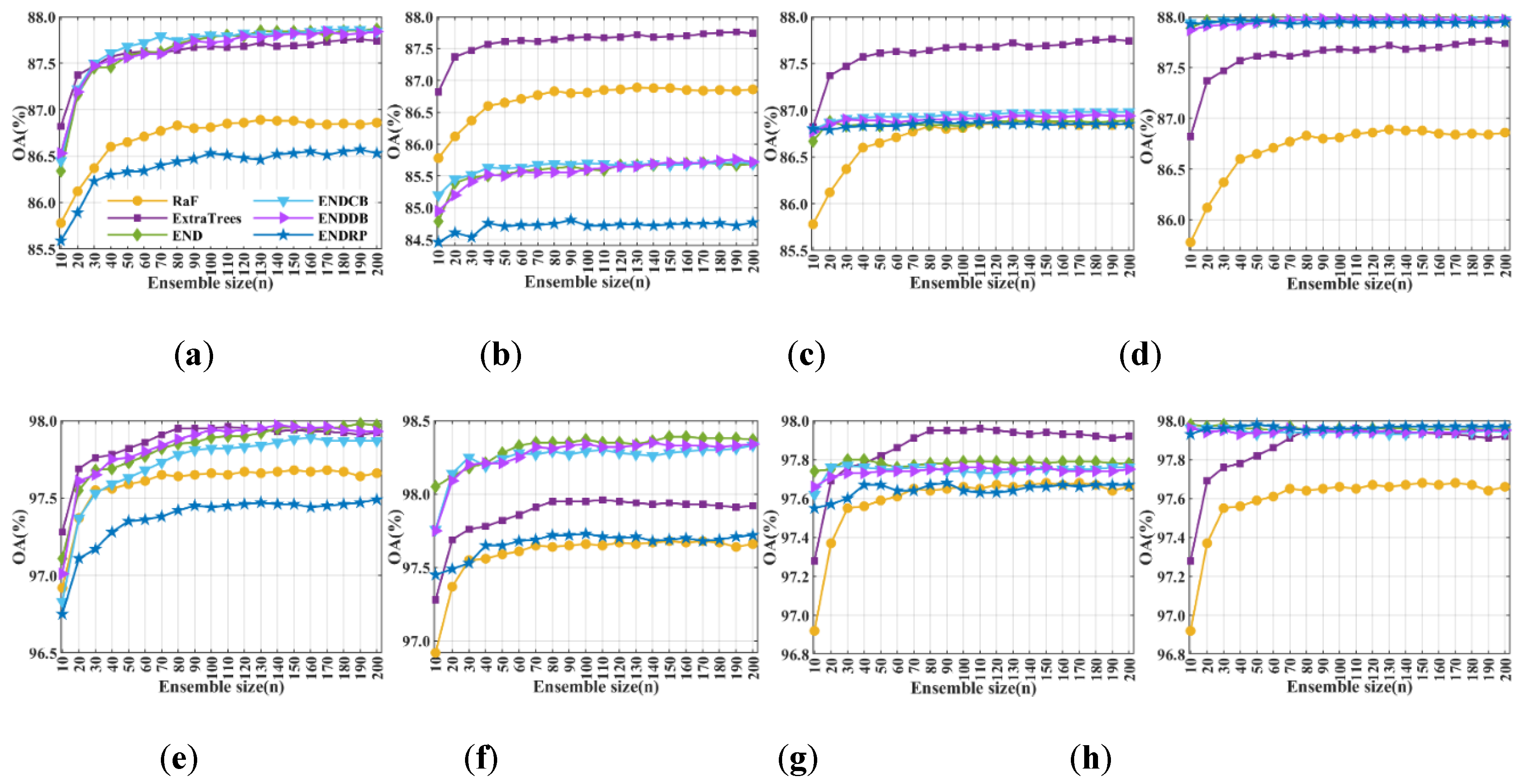
3.2.1. Classification Accuracy
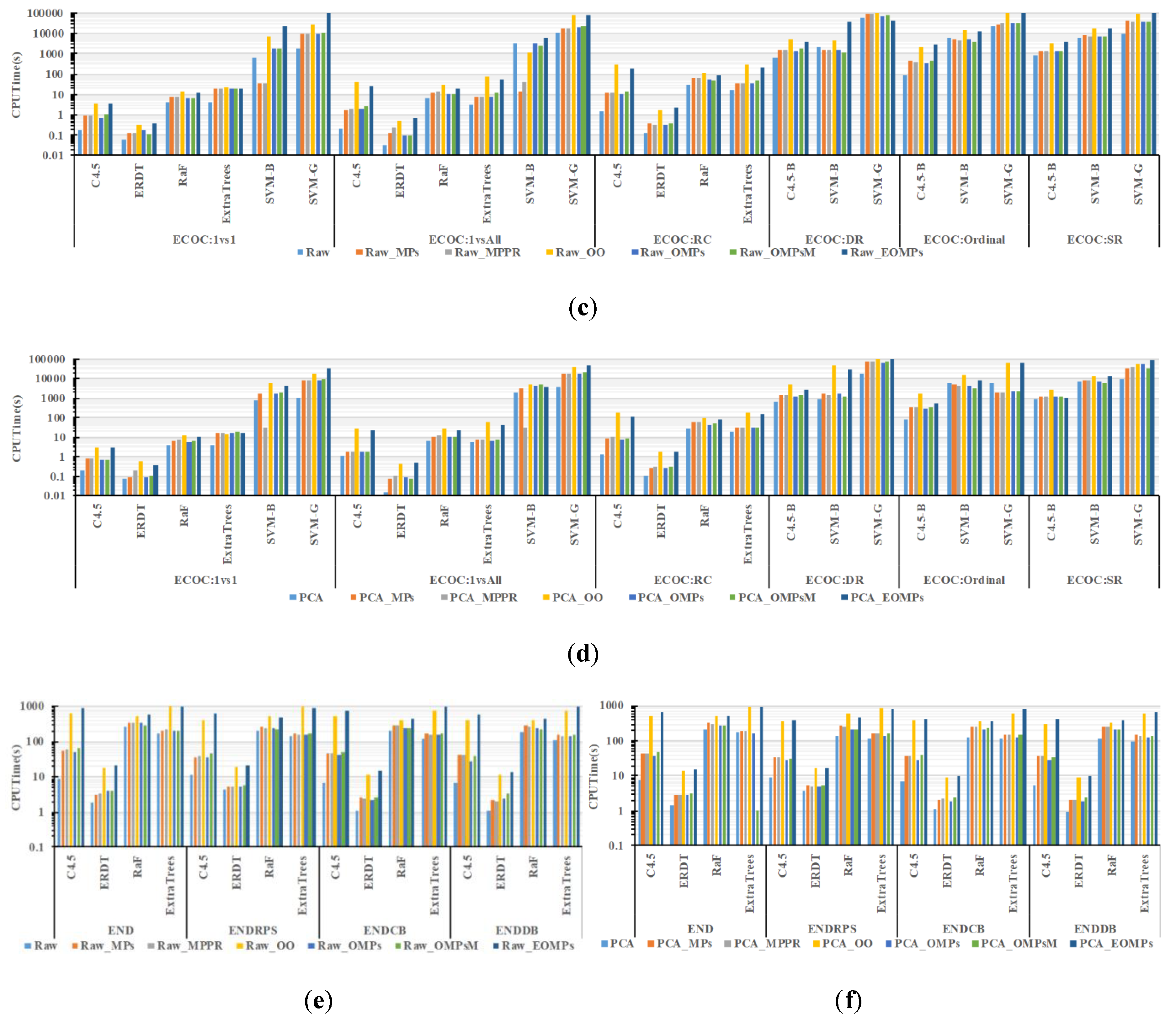
3.2.2. Computational Efficiency
3.2.3. Robustness to the Data Dimensionality
3.3. Final Vegetation Map
4. Discussion
5. Conclusions
Author Contributions
Funding
Acknowledgments
Conflicts of Interest
References
- Chen, Z.; Elvidge, C.D.; Groeneveld, D.P. Monitoring seasonal dynamics of arid land vegetation using AVIRIS data. Remote Sens. Environ. 1998, 65, 255–266. [Google Scholar] [CrossRef]
- Clark, J.S.; Bell, D.M.; Kwit, M.C.; Zhu, K. Competition-interaction landscapes for the joint response of forests to climate change. Glob. Chang. Biol. 2014, 20, 1979–1991. [Google Scholar] [CrossRef] [PubMed]
- Wu, D.; Zhao, X.; Liang, S.; Zhou, T.; Huang, K.; Tang, B.; Zhao, W. Time-lag effects of global vegetation responses to climate change. Glob. Chang. Biol. 2015, 21, 3520–3531. [Google Scholar] [CrossRef] [PubMed]
- Olefeldt, D.; Goswami, S.; Grosse, G.; Hayes, D.; Hugelius, G.; Kuhry, P.; McGuire, A.D.; Romanovsky, V.E.; Sannel, A.B.K.; Schuur, E.A.G.; et al. Circumpolar distribution and carbon storage of thermokarst landscapes. Nat. Commun. 2016, 7, 13043. [Google Scholar] [CrossRef]
- Fleischer, E.; Khashimov, I.; Hölzel, N.; Klemm, O. Carbon exchange fluxes over peatlands in Western Siberia: Possible feedback between land-use change and climate change. Sci. Total Environ. 2016, 545, 424–433. [Google Scholar] [CrossRef] [PubMed]
- Tian, H.; Cao, C.; Chen, W.; Bao, S.; Yang, B.; Myneni, R.B. Response of vegetation activity dynamic to climatic change and ecological restoration programs in Inner Mongolia from 2000 to 2012. Ecol. Eng. 2015, 82, 276–289. [Google Scholar] [CrossRef]
- Jiang, L.; Bao, A.; Guo, H.; Ndayisaba, F. Vegetation dynamics and responses to climate change and human activities in Central Asia. Sci. Total Environ. 2017, 599, 967–980. [Google Scholar] [CrossRef] [PubMed]
- Zhang, Y.; Zhang, C.; Wang, Z.; Chen, Y.; Gang, C.; An, R.; Li, J. Vegetation dynamics and its driving forces from climate change and human activities in the Three-River Source Region, China from 1982 to 2012. Sci. Total Environ. 2016, 563, 210–220. [Google Scholar] [CrossRef]
- Kerr, J.T.; Ostrovsky, M. From space to species: Ecological applications for remote sensing. Trends Ecol. Evol. 2003, 18, 299–305. [Google Scholar] [CrossRef]
- Turner, W.; Spector, S.; Gardiner, N.; Fladeland, M.; Sterling, E.; Steininger, M. Remote sensing for biodiversity science and conservation. Trends Ecol. Evol. 2003, 18, 306–314. [Google Scholar] [CrossRef]
- Madonsela, S.; Cho, M.A.; Ramoelo, A.; Mutanga, O. Remote sensing of species diversity using Landsat 8 spectral variables. ISPRS J. Photogramm. Remote Sens. 2017, 133, 116–127. [Google Scholar] [CrossRef] [Green Version]
- Gould, W. Remote sensing of vegetation, plant species richness, and regional biodiversity hotspots. Ecol. Appl. 2000, 10, 1861–1870. [Google Scholar] [CrossRef]
- Barbier, N.; Couteron, P.; Lejoly, J.; Deblauwe, V.; Lejeune, O. Self-organized vegetation patterning as a fingerprint of climate and human impact on semi-arid ecosystems. J. Ecol. 2006, 94, 537–547. [Google Scholar] [CrossRef]
- Zimmermann, N.E.; Edwards, T.C.; Moisen, G.G.; Frescino, T.S.; Blackard, J.A. Remote sensing-based predictors improve distribution models of rare, early successional and broadleaf tree species in Utah. J. Appl. Ecol. 2007, 44, 1057–1067. [Google Scholar] [CrossRef] [PubMed] [Green Version]
- Xie, Y.; Sha, Z.; Yu, M. Remote sensing imagery in vegetation mapping: A review. J. Plant Ecol. 2008, 1, 9–23. [Google Scholar] [CrossRef]
- Gaitan, J.J.; Oliva, G.E.; Bran, D.E.; Maestre, F.T.; Aguiar, M.R.; Jobbagy, E.G.; Buono, G.G.; Ferrante, D.; Nakamatsu, V.B.; Ciari, G.; et al. Vegetation structure is as important as climate for explaining ecosystem function across Patagonian rangelands. J. Ecol. 2014, 102, 1419–1428. [Google Scholar] [CrossRef] [Green Version]
- Waltari, E.; Schroeder, R.; McDonald, K.; Anderson, R.P.; Carnaval, A. Bioclimatic variables derived from remote sensing: Assessment and application for species distribution modelling. Methods Ecol. Evol. 2014, 5, 1033–1042. [Google Scholar] [CrossRef]
- Tian, F.; Brandt, M.; Liu, Y.Y.; Verger, A.; Tagesson, T.; Diouf, A.A.; Rasmussen, K.; Mbow, C.; Wang, Y.; Fensholt, R. Remote sensing of vegetation dynamics in drylands: Evaluating vegetation optical depth (VOD) using AVHRR NDVI and in situ green biomass data over West African Sahel. Remote Sens. Environ. 2016, 177, 265–276. [Google Scholar] [CrossRef] [Green Version]
- Mildrexler, D.J.; Zhao, M.; Running, S.W. Testing a MODIS global disturbance index across North America. Remote Sens. Environ. 2009, 113, 2103–2117. [Google Scholar] [CrossRef]
- Pettorelli, N.; Laurance, W.F.; O’Brien, T.G.; Wegmann, M.; Nagendra, H.; Turner, W. Satellite remote sensing for applied ecologists: Opportunities and challenges. J. Appl. Ecol. 2014, 51, 839–848. [Google Scholar] [CrossRef]
- Sulla-Menashe, D.; Kennedy, R.E.; Yang, Z.; Braaten, J.; Krankina, O.N.; Friedl, M.A. Detecting forest disturbance in the Pacific Northwest from MODIS time series using temporal segmentation. Remote Sens. Environ. 2014, 151, 114–123. [Google Scholar] [CrossRef]
- McDowell, N.G.; Coops, N.C.; Beck, P.S.; Chambers, J.Q.; Gangodagamage, C.; Hicke, J.A.; Huang, C.Y.; Kennedy, R.; Krofcheck, D.J.; Litvak, M.; et al. Global satellite monitoring of climate-induced vegetation disturbances. Trends Plant Sci. 2015, 20, 114–123. [Google Scholar] [CrossRef] [PubMed]
- Rhodes, C.J.; Henrys, P.; Siriwardena, G.M.; Whittingham, M.J.; Norton, L.R. The relative value of field survey and remote sensing for biodiversity assessment. Methods Ecol. Evol. 2015, 6, 772–781. [Google Scholar] [CrossRef]
- Assal, T.J.; Anderson, P.J.; Sibold, J. Spatial and temporal trends of drought effects in a heterogeneous semi-arid forest ecosystem. For. Ecol. Manag. 2016, 365, 137–151. [Google Scholar] [CrossRef] [Green Version]
- Harvey, K.R.; Hill, G.J.E. Vegetation mapping of a tropical freshwater swamp in the Northern Territory, Australia: A comparison of aerial photography, Landsat TM and SPOT satellite imagery. Int. J. Remote Sens. 2001, 22, 2911–2925. [Google Scholar] [CrossRef]
- Brown, M.E.; Pinzón, J.E.; Didan, K.; Morisette, J.T.; Tucker, C.J. Evaluation of the consistency of long-term NDVI time series derived from AVHRR, SPOT-vegetation, SeaWiFS, MODIS, and Landsat ETM+ sensors. IEEE Trans. Geosci. Remote Sens. 2006, 44, 1787–1793. [Google Scholar] [CrossRef]
- Vieira, M.A.; Formaggio, A.R.; Rennó, C.D.; Atzberger, C.; Aguiar, D.A.; Mello, M.P. Object based image analysis and data mining applied to a remotely sensed Landsat time-series to map sugarcane over large areas. Remote Sens. Environ. 2012, 123, 553–562. [Google Scholar] [CrossRef]
- Dubovyk, O.; Landmann, T.; Erasmus, B.F.; Tewes, A.; Schellberg, J. Monitoring vegetation dynamics with medium resolution MODIS-EVI time series at sub-regional scale in southern Africa. Int. J. Appl. Earth Obs. Geoinf. 2015, 38, 175–183. [Google Scholar] [CrossRef]
- Anchang, J.Y.; Ananga, E.O.; Pu, R. An efficient unsupervised index based approach for mapping urban vegetation from IKONOS imagery. Int. J. Appl. Earth Obs. Geoinf. 2016, 50, 211–220. [Google Scholar] [CrossRef]
- Su, Y.; Guo, Q.; Fry, D.L.; Collins, B.M.; Kelly, M.; Flanagan, J.P.; Battles, J.J. A vegetation mapping strategy for conifer forests by combining airborne LiDAR data and aerial imagery. Can. J. Remote Sens. 2016, 42, 15. [Google Scholar] [CrossRef]
- da Silveira, H.L.F.; Galvão, L.S.; Sanches, I.D.A.; de Sá, I.B.; Taura, T.A. Use of MSI/Sentinel-2 and airborne LiDAR data for mapping vegetation and studying the relationships with soil attributes in the Brazilian semi-arid region. Int. J. Appl. Earth Obs. Geoinf. 2018, 73, 179–190. [Google Scholar] [CrossRef]
- Vrieling, A.; Meroni, M.; Darvishzadeh, R.; Skidmore, A.K.; Wang, T.; Zurita-Milla, R.; Oosterbeek, K.; O’Connor, B.; Paganini, M. Vegetation phenology from Sentinel-2 and field cameras for a Dutch barrier island. Remote Sens. Environ. 2018, 215, 517–529. [Google Scholar] [CrossRef]
- Saveraid, E.H.; Debinski, D.M.; Kindscher, K.; Jakubauskas, M.E. A comparison of satellite data and landscape variables in predicting bird species occurrences in the Greater Yellowstone Ecosystem, USA. Landsc. Ecol. 2001, 16, 71–83. [Google Scholar] [CrossRef]
- Giri, C.; Ochieng, E.; Tieszen, L.L.; Zhu, Z.; Singh, A.; Loveland, T.; Masek, J.; Duke, N. Status and distribution of mangrove forests of the world using earth observation satellite data. Glob. Ecol. Biogeogr. 2011, 20, 154–159. [Google Scholar] [CrossRef]
- Kachelriess, D.; Wegmann, M.; Gollock, M.; Pettorelli, N. The application of remote sensing for marine protected area management. Ecol. Indic. 2014, 36, 169–177. [Google Scholar] [CrossRef]
- Hansen, M.C.; DeFries, R.S.; Townshend, J.R.; Sohlberg, R. Global land cover classification at 1 km spatial resolution using a classification tree approach. Int. J. Remote Sens. 2000, 21, 1331–1364. [Google Scholar] [CrossRef]
- Bartholome, E.; Belward, A.S. GLC2000: A new approach to global land cover mapping from Earth observation data. Int. J. Remote Sens. 2005, 26, 1959–1977. [Google Scholar] [CrossRef]
- Tateishi, R.; Uriyangqai, B.; Al-Bilbisi, H.; Ghar, M.A.; Tsend-Ayush, J.; Kobayashi, T.; Kasimu, A.; Hoan, N.T.; Shalaby, A.; Alsaaideh, B.; et al. Production of global land cover data–GLCNMO. Int. J. Digit. Earth 2011, 4, 22–49. [Google Scholar] [CrossRef]
- Friedl, M.A.; Sulla-Menashe, D.; Tan, B.; Schneider, A.; Ramankutty, N.; Sibley, A.; Huang, X. MODIS Collection 5 global land cover: Algorithm refinements and characterization of new datasets. Remote Sens. Environ. 2010, 114, 168–182. [Google Scholar] [CrossRef]
- Arino, O.; Perez, R.; Ramos Perez, J.J.; Kalogirou, V.; Bontemps, S.; Defourny, P.; Van Bogaert, E. Global land cover map for 2009, European Space Agency (ESA) & Université catholique de Louvain (UCL), PANGAEA. 2012. Available online: https://doi.pangaea.de/10.1594/PANGAEA.787668 (accessed on 30 July 2019).
- Chen, J.; Liao, A.; Cao, X.; Chen, L.; Chen, X.; He, C.; Han, G.; Peng, S.; Lu, M.; Zhang, W. Global land cover mapping at 30 m resolution: A POK-based operational approach. ISPRS J. Photogramm. Remote Sens. 2015, 103, 7–27. [Google Scholar] [CrossRef]
- Hansen, M.C.; Reed, B. A comparison of the IGBP DISCover and University of Maryland 1 km global land cover products. Int. J. Remote Sens. 2000, 21, 1365–1373. [Google Scholar] [CrossRef]
- Myneni, R.B.; Hoffman, S.; Knyazikhin, Y.; Privette, J.L.; Glassy, J.; Tian, Y.; Wang, Y.; Song, X.; Zhang, Y.; Smith, G.R.; et al. Global products of vegetation leaf area and fraction absorbed PAR from year one of MODIS data. Remote Sens. Environ. 2002, 83, 214–231. [Google Scholar] [CrossRef] [Green Version]
- Hansen, M.C.; DeFries, R.S.; Townshend, J.R.G.; Carroll, M.; Dimiceli, C.; Sohlberg, R.A. Global percent tree cover at a spatial resolution of 500 meters: First results of the MODIS vegetation continuous fields algorithm. Earth Interact. 2003, 7, 1–15. [Google Scholar] [CrossRef]
- Ganguly, S.; Friedl, M.A.; Tan, B.; Zhang, X.; Verma, M. Land surface phenology from MODIS: Characterization of the Collection 5 global land cover dynamics product. Remote Sens. Environ. 2010, 114, 1805–1816. [Google Scholar] [CrossRef] [Green Version]
- Gong, P.; Wang, J.; Yu, L.; Zhao, Y.; Zhao, Y.; Liang, L.; Niu, Z.; Huang, X.; Fu, H.; Liu, S.; et al. Finer resolution observation and monitoring of global land cover: First mapping results with Landsat TM and ETM+ data. Int. J. Remote Sens. 2013, 34, 2607–2654. [Google Scholar] [CrossRef]
- Tuanmu, M.N.; Jetz, W. A global 1-km consensus land-cover product for biodiversity and ecosystem modelling. Glob. Ecol. Biogeogr. 2014, 23, 1031–1045. [Google Scholar] [CrossRef]
- Zhang, H.K.; Roy, D.P. Using the 500 m MODIS land cover product to derive a consistent continental scale 30 m Landsat land cover classification. Remote Sens. Environ. 2017, 197, 15–34. [Google Scholar] [CrossRef]
- Yu, Q.; Hu, Q.; van Vliet, J.; Verburg, P.H.; Wu, W. GlobeLand30 shows little cropland area loss but greater fragmentation in China. Int. J. Appl. Earth Obs. Geoinf. 2018, 66, 37–45. [Google Scholar] [CrossRef]
- Drusch, M.; Del Bello, U.; Carlier, S.; Colin, O.; Fernandez, V.; Gascon, F.; Hoersch, B.; Isola, C.; Laberinti, P.; Meygret, A.; et al. Sentinel-2: ESA’s optical high-resolution mission for GMES operational services. Remote Sens. Environ. 2012, 120, 25–36. [Google Scholar] [CrossRef]
- Frampton, W.J.; Dash, J.; Watmough, G.; Milton, E.J. Evaluating the capabilities of Sentinel-2 for quantitative estimation of biophysical variables in vegetation. ISPRS J. Photogramm. Remote Sens. 2013, 82, 83–92. [Google Scholar] [CrossRef] [Green Version]
- Verrelst, J.; Rivera, J.P.; Leonenko, G.; Alonso, L.; Moreno, J. Optimizing LUT-based RTM inversion for semiautomatic mapping of crop biophysical parameters from Sentinel-2 and-3 data: Role of cost functions. IEEE Trans. Geosci. Remote Sens. 2014, 52, 257–269. [Google Scholar] [CrossRef]
- Kääb, A.; Winsvold, S.H.; Altena, B.; Nuth, C.; Nagler, T.; Wuite, J. Glacier remote sensing using Sentinel-2. part I: Radiometric and geometric performance, and application to ice velocity. Remote Sens. 2016, 8, 598. [Google Scholar]
- Novelli, A.; Aguilar, M.A.; Nemmaoui, A.; Aguilar, F.J.; Tarantino, E. Performance evaluation of object based greenhouse detection from Sentinel-2 MSI and Landsat 8 OLI data: A case study from Almería (Spain). Int. J. Appl. Earth Obs. Geoinf. 2016, 52, 403–411. [Google Scholar] [CrossRef]
- Belgiu, M.; Csillik, O. Sentinel-2 cropland mapping using pixel-based and object-based time-weighted dynamic time warping analysis. Remote Sens. Environ. 2018, 204, 509–523. [Google Scholar] [CrossRef]
- Griffiths, P.; Nendel, C.; Hostert, P. Intra-annual reflectance composites from Sentinel-2 and Landsat for national-scale crop and land cover mapping. Remote Sens. Environ. 2019, 220, 135–151. [Google Scholar] [CrossRef]
- Chan, J.C.W.; Paelinckx, D. Evaluation of Random Forest and Adaboost tree-based ensemble classification and spectral band selection for ecotope mapping using airborne hyperspectral imagery. Remote Sens. Environ. 2008, 112, 2999–3011. [Google Scholar] [CrossRef]
- Naidoo, L.; Cho, M.A.; Mathieu, R.; Asner, G. Classification of savanna tree species, in the Greater Kruger National Park region, by integrating hyperspectral and LiDAR data in a Random Forest data mining environment. ISPRS J. Photogramm. Remote Sens. 2012, 69, 167–179. [Google Scholar] [CrossRef]
- Kumar, P.; Gupta, D.K.; Mishra, V.N.; Prasad, R. Comparison of support vector machine, artificial neural network, and spectral angle mapper algorithms for crop classification using LISS IV data. Int. J. Remote Sens. 2015, 36, 1604–1617. [Google Scholar] [CrossRef]
- Omer, G.; Mutanga, O.; Abdel-Rahman, E.M.; Adam, E. Performance of support vector machines and artificial neural network for mapping endangered tree species using WorldView-2 data in Dukuduku forest, South Africa. IEEE J. Sel. Top. Appl. Earth Obs. Remote Sens. 2015, 8, 4825–4840. [Google Scholar] [CrossRef]
- Olofsson, P.; Foody, G.M.; Herold, M.; Stehman, S.V.; Woodcock, C.E.; Wulder, M.A. Good practices for estimating area and assessing accuracy of land change. Remote Sens. Environ. 2014, 148, 42–57. [Google Scholar] [CrossRef]
- Samat, A.; Li, J.; Liu, S.; Du, P.; Miao, Z.; Luo, J. Improved hyperspectral image classification by active learning using pre-designed mixed pixels. Pattern Recognit. 2016, 51, 43–58. [Google Scholar] [CrossRef]
- Mas, J.F.; Flores, J.J. The application of artificial neural networks to the analysis of remotely sensed data. Int. J. Remote Sens. 2008, 29, 617–663. [Google Scholar] [CrossRef]
- Mountrakis, G.; Im, J.; Ogole, C. Support vector machines in remote sensing: A review. ISPRS J. Photogramm. Remote Sens. 2011, 66, 247–259. [Google Scholar] [CrossRef]
- Maulik, U.; Chakraborty, D. Remote sensing image classification: A survey of support-vector-machine-based advanced techniques. IEEE Geosci. Remote Sens. Mag. 2017, 5, 33–52. [Google Scholar] [CrossRef]
- Samat, A.; Du, P.; Liu, S.; Li, J.; Cheng, L. E2LMs: Ensemble Extreme Learning Machines for Hyperspectral Image Classification. IEEE J. Sel. Top. Appl. Earth Obs. Remote Sens. 2014, 7, 1060–1069. [Google Scholar] [CrossRef]
- Xu, M.; Watanachaturaporn, P.; Varshney, P.K.; Arora, M.K. Decision tree regression for soft classification of remote sensing data. Remote Sens. Environ. 2005, 97, 322–336. [Google Scholar] [CrossRef]
- Du, P.; Samat, A.; Waske, B.; Liu, S.; Li, Z. Random forest and rotation forest for fully polarized SAR image classification using polarimetric and spatial features. ISPRS J. Photogramm. Remote Sens. 2015, 105, 38–53. [Google Scholar] [CrossRef]
- Belgiu, M.; Drăguţ, L. Random forest in remote sensing: A review of applications and future directions. ISPRS J. Photogramm. Remote Sens. 2016, 114, 24–31. [Google Scholar] [CrossRef]
- Zhang, L.; Zhang, L.; Du, B. Deep learning for remote sensing data: A technical tutorial on the state of the art. IEEE Geosci. Remote Sens. Mag. 2016, 4, 22–40. [Google Scholar] [CrossRef]
- Zhu, X.X.; Tuia, D.; Mou, L.; Xia, G.S.; Zhang, L.; Xu, F.; Fraundorfer, F. Deep learning in remote sensing: A comprehensive review and list of resources. IEEE Geosci. Remote Sens. Mag. 2017, 5, 8–36. [Google Scholar] [CrossRef]
- Dietterich, T.G.; Bakiri, G. Solving multiclass learning problems via error-correcting output codes. J. Artif. Intell. Res. 1994, 2, 263–286. [Google Scholar] [CrossRef]
- Allwein, E.L.; Schapire, R.E.; Singer, Y. Reducing multiclass to binary: A unifying approach for margin classifiers. J. Mach. Learn. Res. 2000, 1, 113–141. [Google Scholar]
- Duarte-Villaseñor, M.M.; Carrasco-Ochoa, J.A.; Martínez-Trinidad, J.F.; Flores-Garrido, M. Nested dichotomies based on clustering. In Iberoamerican Congress on Pattern Recognition; Springer: Berlin/Heidelberg, Germany, September 2012; pp. 162–169. [Google Scholar]
- Dong, L.; Frank, E.; Kramer, S. Ensembles of balanced nested dichotomies for multi-class problems. In European Conference on Principles of Data Mining and Knowledge Discovery; Springer: Berlin/Heidelberg, Germany, October 2005; pp. 84–95. [Google Scholar]
- Foody, G.M.; Mathur, A. A relative evaluation of multiclass image classification by support vector machines. IEEE Trans. Geosci. Remote Sens. 2004, 42, 1335–1343. [Google Scholar] [CrossRef] [Green Version]
- Plaza, A.; Benediktsson, J.A.; Boardman, J.W.; Brazile, J.; Bruzzone, L.; Camps-Valls, G.; Chanussot, J.; Fauvel, M.; Gamba, P.; Gualtieri, A.; et al. Recent advances in techniques for hyperspectral image processing. Remote Sens. Environ. 2009, 113, S110–S122. [Google Scholar] [CrossRef]
- Shao, Y.; Lunetta, R.S. Comparison of support vector machine, neural network, and CART algorithms for the land-cover classification using limited training data points. ISPRS J. Photogramm. Remote Sens. 2012, 70, 78–87. [Google Scholar] [CrossRef]
- Hüllermeier, E.; Vanderlooy, S. Combining predictions in pairwise classification: An optimal adaptive voting strategy and its relation to weighted voting. Pattern Recognit. 2010, 43, 128–142. [Google Scholar] [CrossRef] [Green Version]
- Passerini, A.; Pontil, M.; Frasconi, P. New results on error correcting output codes of kernel machines. IEEE Trans. Neural Netw. 2004, 15, 45–54. [Google Scholar] [CrossRef]
- Pujol, O.; Radeva, P.; Vitria, J. Discriminant ECOC: A heuristic method for application dependent design of error correcting output codes. IEEE Trans. Pattern Anal. Mach. Intell. 2006, 28, 1007–1012. [Google Scholar] [CrossRef]
- Escalera, S.; Pujol, O.; Radeva, P. On the decoding process in ternary error-correcting output codes. IEEE Trans. Pattern Anal. Mach. Intell. 2010, 32, 120–134. [Google Scholar] [CrossRef]
- Pal, M. Class decomposition Approaches for land cover classification: A comparative study. In Proceedings of the IEEE International Geoscience and Remote Sensing Symposium, IGARSS 2006, Denver, CO, USA, 31 July–4 August 2006; pp. 2731–2733. [Google Scholar]
- Mera, D.; Fernández-Delgado, M.; Cotos, J.M.; Viqueira, J.R.R.; Barro, S. Comparison of a massive and diverse collection of ensembles and other classifiers for oil spill detection in sar satellite images. Neural Comput. Appl. 2017, 28, 1101–1117. [Google Scholar] [CrossRef]
- Frank, E.; Kramer, S. Ensembles of nested dichotomies for multi-class problems. In Proceedings of the Twenty-First International Conference on Machine Learning, Banff, AB, Canada, 4–8 July 2004; p. 39. [Google Scholar]
- Rodríguez, J.J.; García-Osorio, C.; Maudes, J. Forests of nested dichotomies. Pattern Recognit. Lett. 2010, 31, 125–132. [Google Scholar] [CrossRef]
- Quinlan, J.R. Bagging, boosting, and C4. 5. In Proceedings of the AAAI’96 Proceedings of the Thirteenth National Conference on Artificial Intelligence, Portland, OR, USA, 4–8 August 1996; Volume 1, pp. 725–730. [Google Scholar]
- Rätsch, G.; Onoda, T.; Müller, K.R. Soft margins for AdaBoost. Mach. Learn. 2001, 42, 287–320. [Google Scholar] [CrossRef]
- Breiman, L. Random forests. Mach. Learn. 2001, 45, 5–32. [Google Scholar] [CrossRef]
- Rodriguez, J.J.; Kuncheva, L.I.; Alonso, C.J. Rotation forest: A new classifier ensemble method. IEEE Trans. Pattern Anal. Mach. Intell. 2006, 28, 1619–1630. [Google Scholar] [CrossRef] [PubMed]
- Geurts, P.; Ernst, D.; Wehenkel, L. Extremely randomized trees. Mach. Learn. 2006, 63, 3–42. [Google Scholar] [CrossRef] [Green Version]
- Cortes, C.; Vapnik, V. Support vector machine. Mach. Learn. 1995, 20, 273–297. [Google Scholar] [CrossRef]
- Fauvel, M.; Tarabalka, Y.; Benediktsson, J.A.; Chanussot, J.; Tilton, J.C. Advances in spectral-spatial classification of hyperspectral images. Proc. IEEE 2013, 101, 652–675. [Google Scholar] [CrossRef]
- Li, M.; Zang, S.; Zhang, B.; Li, S.; Wu, C. A review of remote sensing image classification techniques: The role of spatio-contextual information. Eur. J. Remote Sens. 2014, 47, 389–411. [Google Scholar] [CrossRef]
- Chen, Y.; Zhao, X.; Jia, X. Spectral-spatial classification of hyperspectral data based on deep belief network. IEEE J. Sel. Top. Appl. Earth Obs. Remote Sens. 2015, 8, 2381–2392. [Google Scholar] [CrossRef]
- He, L.; Li, J.; Liu, C.; Li, S. Recent advances on spectral-spatial hyperspectral image classification: An overview and new guidelines. IEEE Trans. Geosci. Remote Sens. 2018, 56, 1579–1597. [Google Scholar] [CrossRef]
- Liao, W.; Chanussot, J.; Dalla Mura, M.; Huang, X.; Bellens, R.; Gautama, S.; Philips, W. Taking Optimal Advantage of Fine Spatial Resolution: Promoting partial image reconstruction for the morphological analysis of very-high-resolution images. IEEE Geosci. Remote Sens. Mag. 2017, 5, 8–28. [Google Scholar] [CrossRef] [Green Version]
- Samat, A.; Persello, C.; Liu, S.; Li, E.; Miao, Z.; Abuduwaili, J. Classification of VHR Multispectral Images Using ExtraTrees and Maximally Stable Extremal Region-Guided Morphological Profile. IEEE J. Sel. Top. Appl. Earth Obs. Remote Sens. 2018, 11, 3179–3195. [Google Scholar] [CrossRef]
- Samat, A.; Liu, S.; Persello, C.; Li, E.; Miao, Z.; Abuduwaili, J. Evaluation of ForestPA for VHR RS image classification using spectral and superpixel-guided morphological profiles. Eur. J. Remote Sens. 2019, 52, 107–121. [Google Scholar] [CrossRef] [Green Version]
- Blaschke, T. Object based image analysis for remote sensing. ISPRS J. Photogramm. Remote Sens. 2010, 65, 2–16. [Google Scholar] [CrossRef] [Green Version]
- Blaschke, T.; Hay, G.J.; Kelly, M.; Lang, S.; Hofmann, P.; Addink, E.; Queiroz Feitosa, R.; van der Meer, F.; van der Werff, H.; Tiede, D.; et al. Geographic object-based image analysis–towards a new paradigm. ISPRS J. Photogramm. Remote Sens. 2014, 87, 180–191. [Google Scholar] [CrossRef] [PubMed]
- Ma, L.; Li, M.; Ma, X.; Cheng, L.; Du, P.; Liu, Y. A review of supervised object-based land-cover image classification. ISPRS J. Photogramm. Remote Sens. 2017, 130, 277–293. [Google Scholar] [CrossRef]
- Kezer, K.; Matsuyama, H. Decrease of river runoff in the Lake Balkhash basin in Central Asia. Hydrol. Process. Int. J. 2006, 20, 1407–1423. [Google Scholar] [CrossRef]
- Propastin, P.A. Simple model for monitoring Balkhash Lake water levels and Ili River discharges: Application of remote sensing. Lakes Reserv. Res. Manag. 2008, 13, 77–81. [Google Scholar] [CrossRef]
- Propastin, P. Problems of water resources management in the drainage basin of Lake Balkhash with respect to political development. In Climate Change and the Sustainable Use of Water Resources; Springer: Berlin/Heidelberg, Germany, 2012; pp. 449–461. [Google Scholar]
- Petr, T.; Mitrofanov, V.P. The impact on fish stocks of river regulation in Central Asia and Kazakhstan. Lakes Reserv. Res. Manag. 1998, 3, 143–164. [Google Scholar] [CrossRef]
- Bai, J.; Chen, X.; Li, J.; Yang, L.; Fang, H. Changes in the area of inland lakes in arid regions of central Asia during the past 30 years. Environ. Monit. Assess. 2011, 178, 247–256. [Google Scholar] [CrossRef]
- Klein, I.; Gessner, U.; Kuenzer, C. Regional land cover mapping and change detection in Central Asia using MODIS time-series. Appl. Geogr. 2012, 35, 219–234. [Google Scholar] [CrossRef]
- Chen, X.; Bai, J.; Li, X.; Luo, G.; Li, J.; Li, B.L. Changes in land use/land cover and ecosystem services in Central Asia during 1990. Curr. Opin. Environ. Sustain. 2013, 5, 116–127. [Google Scholar] [CrossRef]
- De Beurs, K.M.; Henebry, G.M.; Owsley, B.C.; Sokolik, I. Using multiple remote sensing perspectives to identify and attribute land surface dynamics in Central Asia 2001. Remote Sens. Environ. 2015, 170, 48–61. [Google Scholar] [CrossRef]
- Zhang, C.; Lu, D.; Chen, X.; Zhang, Y.; Maisupova, B.; Tao, Y. The spatiotemporal patterns of vegetation coverage and biomass of the temperate deserts in Central Asia and their relationships with climate controls. Remote Sens. Environ. 2016, 175, 271–281. [Google Scholar] [CrossRef]
- Leathart, T.; Pfahringer, B.; Frank, E. Building ensembles of adaptive nested dichotomies with random-pair selection. In Joint European Conference on Machine Learning and Knowledge Discovery in Data Bases; Springer: Cham, Switzerland, 2016; pp. 179–194. [Google Scholar]
- Leathart, T.; Frank, E.; Pfahringer, B.; Holmes, G. Ensembles of Nested Dichotomies with Multiple Subset Evaluation. arXiv 2018, arXiv:1809.02740. [Google Scholar]
- Wever, M.; Mohr, F.; Hüllermeier, E. Ensembles of evolved nested dichotomies for classification. In Proceedings of the Genetic and Evolutionary Computation Conference, Kyoto, Japan, 15–19 July 2018; pp. 561–568. [Google Scholar]
- Myint, S.W.; Gober, P.; Brazel, A.; Grossman-Clarke, S.; Weng, Q. Per-pixel vs. object-based classification of urban land cover extraction using high spatial resolution imagery. Remote Sens. Environ. 2011, 115, 1145–1161. [Google Scholar] [CrossRef]
- Drăguţ, L.; Eisank, C. Automated object-based classification of topography from SRTM data. Geomorphology 2012, 141, 21–33. [Google Scholar] [CrossRef]
- Drăguţ, L.; Csillik, O.; Eisank, C.; Tiede, D. Automated parameterisation for multi-scale image segmentation on multiple layers. ISPRS J. Photogramm. Remote Sens. 2014, 88, 119–127. [Google Scholar] [CrossRef]
- Benz, U.C.; Hofmann, P.; Willhauck, G.; Lingenfelder, I.; Heynen, M. Multi-resolution, object-oriented fuzzy analysis of remote sensing data for GIS-ready information. ISPRS J. Photogramm. Remote Sens. 2004, 58, 239–258. [Google Scholar] [CrossRef]
- Kim, M.; Warner, T.A.; Madden, M.; Atkinson, D.S. Multi-scale GEOBIA with very high spatial resolution digital aerial imagery: Scale, texture and image objects. Int. J. Remote Sens. 2011, 32, 2825–2850. [Google Scholar] [CrossRef]
- Drǎguţ, L.; Tiede, D.; Levick, S.R. ESP: A tool to estimate scale parameter for multiresolution image segmentation of remotely sensed data. Int. J. Geogr. Inf. Sci. 2010, 24, 859–871. [Google Scholar] [CrossRef]
- Benediktsson, J.A.; Palmason, J.A.; Sveinsson, J.R. Classification of hyperspectral data from urban areas based on extended morphological profiles. IEEE Trans. Geosci. Remote Sens. 2005, 43, 480–491. [Google Scholar] [CrossRef]
- Fauvel, M.; Benediktsson, J.A.; Chanussot, J.; Sveinsson, J.R. Spectral and spatial classification of hyperspectral data using SVMs and morphological profiles. IEEE Trans. Geosci. Remote Sens. 2008, 46, 3804–3814. [Google Scholar] [CrossRef]
- Dalla Mura, M.; Villa, A.; Benediktsson, J.A.; Chanussot, J.; Bruzzone, L. Classification of hyperspectral images by using extended morphological attribute profiles and independent component analysis. IEEE Geosci. Remote Sens. Lett. 2011, 8, 542–546. [Google Scholar] [CrossRef]
- Plaza, A.; Martinez, P.; Perez, R.; Plaza, J. A new approach to mixed pixel classification of hyperspectral imagery based on extended morphological profiles. Pattern Recognit. 2004, 37, 1097–1116. [Google Scholar] [CrossRef]
- Aptoula, E.; Lefèvre, S. A comparative study on multivariate mathematical morphology. Pattern Recognit. 2007, 40, 2914–2929. [Google Scholar] [CrossRef] [Green Version]
- Samat, A.; Gamba, P.; Liu, S.; Miao, Z.; Li, E.; Abuduwaili, J. Quad-PolSAR data classification using modified random forest algorithms to map halophytic plants in arid areas. Int. J. Appl. Earth Obs. Geoinf. 2018, 73, 503–521. [Google Scholar] [CrossRef]
- Snoek, J.; Larochelle, H.; Adams, R.P. Practical bayesian optimization of machine learning algorithms. In Proceedings of the Advances in Neural Information Processing Systems, Lake Tahoe, NV, USA, 3–6 December 2012; pp. 2951–2959, Curran Associates. [Google Scholar]
- Du, P.; Xia, J.; Zhang, W.; Tan, K.; Liu, Y.; Liu, S. Multiple classifier system for remote sensing image classification: A Review. Sensors (Basel) 2012, 12, 4764–4792. [Google Scholar] [CrossRef]
- Samat, A.; Gamba, P.; Du, P.; Luo, J. Active extreme learning machines for quad-polarimetric SAR imagery classification. Int. J. Appl. Earth Obs. Geoinf. 2015, 35, 305–319. [Google Scholar] [CrossRef]
- Vihervaara, P.; Auvinen, A.P.; Mononen, L.; Törmä, M.; Ahlroth, P.; Anttila, S.; Böttcher, K.; Forsius, M.; Heino, J.; Koskelainen, M.; et al. How essential biodiversity variables and remote sensing can help national biodiversity monitoring. Glob. Ecol. Conserv. 2017, 10, 43–59. [Google Scholar] [CrossRef]
- Gholizadeh, H.; Gamon, J.A.; Zygielbaum, A.I.; Wang, R.; Schweiger, A.K.; Cavender-Bares, J. Remote sensing of biodiversity: Soil correction and data dimension reduction methods improve assessment of α-diversity (species richness) in prairie ecosystems. Remote Sens. Environ. 2018, 206, 240–253. [Google Scholar] [CrossRef]
- Gholizadeh, H.; Gamon, J.A.; Townsend, P.A.; Zygielbaum, A.I.; Helzer, C.J.; Hmimina, G.Y.; Moore, R.M.; Schweiger, A.K.; Cavender-Bares, J. Detecting prairie biodiversity with airborne remote sensing. Remote Sens. Environ. 2019, 221, 38–49. [Google Scholar] [CrossRef]


| Acronyms | Full Name | Acronyms | Full Name |
|---|---|---|---|
| AA | Average accuracy | MSIL1C | MultiSpectral Instrument Level-1C |
| AFs | Attribute filters | MSER-MPs | Maximally stable extremal region-guided MPs |
| ANNs | Artificial neural networks | ND | Nested dichotomies |
| AVHRR | Advanced VHR Radiometer | NDBC | ND based on clustering |
| CBR | Closing by reconstruction | NDCB | ND with class balancing |
| CVRFR | Classification via RaF regression | NDDB | ND with data balancing |
| DL | Deep learning | NDFC | ND with further centroid |
| DNNs | Deep neural networks | NDRPS | ND with random-pair selection |
| DTs | Decision trees | OA | Overall accuracy |
| ECOC | Error-correcting output code | OBIA | Object-based image analysis |
| EERDTs | Ensemble of ERDTs | OBR | Opening by reconstruction |
| EL | Ensemble learning | OBPR | Opening by partial reconstruction |
| ELM | Extreme learning machine | OLI | Operational Land Imager |
| END | Ensembles of ND | OMPs | Object-guided MPs |
| ENDBC | Ensemble of NDBC | OMPsM | OMPs with mean values |
| ENDCB | Ensemble of NDCB | OO | Object-oriented |
| ENDDB | Ensemble of NDDB | OOBR | Object guided OBR |
| ENDRPS | Ensemble of NDRPS | PCA | Principal component analysis |
| END-ERDT | END with ERDT | RaF | Random forest |
| EOMPs | Extended object-guided MPs | RBF | Radial basis function |
| ERDT | Extremely randomized DT | ROI | Region of interest |
| ESA | European Space Agency | RoF | Rotation forest |
| ETM | Enhanced Thematic Mapper | SE | Structural element |
| ExtraTrees | Extremely randomized trees | SEOM | ESA’s Scientific Exploration of Operational Missions |
| EVI | Enhanced vegetation index | SNAP | Sentinel Application Platform |
| GEOBIA | Geographic OBIA | SPOT | Satellite for Observation of Earth |
| GPS | Global positioning system | SR | Sparse representation |
| HR | High resolution | SRM | Structural risk minimization |
| LDA | Linear discriminate analysis | SVM | Support vector machine |
| LR | Logistic regression | SVM-B | SVM with Bayes optimization |
| ML | Machine learning | SVM-G | SVM with grid-search optimization |
| MM | Mathematical morphology | SWIR | Short wave infrared |
| MPs | Morphological profiles | UA | User accuracy |
| MPPR | MPs with partial reconstruction | UMD | University of Maryland |
| MRFs | Markov random fields | TOA | Top-of-atmosphere |
| MRS | Nulti-resolution segmentation | VHR | Very high resolution |
| MODIS | Moderate Resolution Imaging Spectroradiometer | VI | Vegetation index |
| MSI | MultiSpectral Instrument | VNIR | Visible and the near-infrared |
| LC Types | 1 | 2 | 3 | 4 | 5 | 6 | 7 | 8 | 9 | 10 | 11 | 12 | 13 | 14 | 15 | 16 | 17 | 18 | 19 | 20 | 21 | 22 | 23 | Total |
|---|---|---|---|---|---|---|---|---|---|---|---|---|---|---|---|---|---|---|---|---|---|---|---|---|
| ROIs | 253 | 39 | 30 | 17 | 30 | 13 | 6 | 7 | 16 | 1 | 4 | 20 | 9 | 33 | 7 | 6 | 2 | 5 | 19 | 15 | 5 | 8 | 37 | 582 |
| Train | 147 | 230 | 295 | 144 | 325 | 225 | 128 | 19 | 304 | 12 | 92 | 164 | 42 | 277 | 117 | 45 | 27 | 75 | 976 | 171 | 30 | 238 | 475 | 4558 |
| Test | 2794 | 4366 | 5600 | 2726 | 6180 | 4269 | 2428 | 352 | 5768 | 218 | 1753 | 3113 | 794 | 5256 | 2226 | 852 | 516 | 1429 | 18542 | 3246 | 560 | 4523 | 9021 | 86532 |
| Total | 2941 | 4596 | 5895 | 2870 | 6505 | 4494 | 2556 | 371 | 6072 | 230 | 1845 | 3277 | 836 | 5533 | 2343 | 897 | 543 | 1504 | 19518 | 3417 | 590 | 4761 | 9496 | 91090 |
| Class No. | END-ERDT | ECOC:1vsAll (SVM-G) | ||||||||||||
|---|---|---|---|---|---|---|---|---|---|---|---|---|---|---|
| Raw | Raw_MPs | Raw_MPPR | Raw_OMPs | Raw_OMPsM | Raw_OO | Raw_EOMPs | Raw | Raw_MPs | Raw_MPPR | Raw_OMPs | Raw_OMPsM | Raw_OO | Raw_EOMPs | |
| 1 | 54.01 | 92.27 | 96.21 | 96.06 | 98.50 | 99.64 | 99.64 | 62.53 | 93.52 | 93.59 | 92.95 | 96.39 | 97.57 | 98.85 |
| 2 | 98.12 | 99.63 | 99.84 | 100.00 | 100.00 | 100.00 | 100.00 | 97.64 | 99.59 | 99.86 | 100.00 | 99.91 | 100.00 | 100.00 |
| 3 | 99.86 | 99.86 | 99.88 | 99.95 | 99.96 | 100.00 | 100.00 | 99.66 | 99.52 | 100.00 | 99.88 | 99.86 | 100.00 | 100.00 |
| 4 | 63.65 | 92.99 | 97.62 | 98.31 | 99.85 | 100.00 | 100.00 | 55.58 | 97.80 | 97.10 | 98.86 | 99.96 | 100.00 | 100.00 |
| 5 | 79.79 | 96.25 | 98.03 | 97.59 | 99.97 | 100.00 | 100.00 | 82.44 | 96.73 | 97.98 | 97.61 | 99.92 | 99.92 | 99.92 |
| 6 | 95.46 | 99.32 | 99.88 | 100.00 | 100.00 | 100.00 | 100.00 | 97.77 | 99.11 | 99.98 | 100.00 | 100.00 | 100.00 | 100.00 |
| 7 | 89.62 | 97.65 | 98.64 | 99.14 | 99.14 | 97.57 | 98.02 | 94.28 | 98.27 | 99.05 | 99.63 | 98.89 | 97.32 | 97.32 |
| 8 | 25.28 | 92.90 | 97.44 | 100.00 | 100.00 | 100.00 | 100.00 | 37.50 | 99.43 | 98.86 | 99.15 | 99.72 | 100.00 | 100.00 |
| 9 | 88.68 | 98.60 | 99.03 | 99.90 | 99.97 | 100.00 | 100.00 | 88.18 | 98.75 | 98.44 | 99.77 | 99.69 | 100.00 | 100.00 |
| 10 | 15.14 | 75.23 | 95.41 | 94.95 | 96.79 | 98.17 | 100.00 | 2.75 | 92.66 | 97.71 | 94.95 | 92.20 | 100.00 | 100.00 |
| 11 | 79.52 | 98.40 | 99.32 | 99.54 | 99.89 | 100.00 | 100.00 | 88.82 | 98.75 | 99.83 | 99.77 | 99.89 | 100.00 | 100.00 |
| 12 | 77.42 | 94.96 | 93.61 | 97.59 | 98.49 | 98.33 | 99.97 | 79.25 | 94.47 | 93.90 | 94.67 | 99.16 | 98.30 | 98.30 |
| 13 | 58.19 | 97.23 | 97.86 | 99.37 | 99.24 | 99.87 | 99.87 | 87.41 | 97.98 | 96.98 | 99.12 | 99.37 | 99.87 | 99.87 |
| 14 | 90.56 | 97.03 | 98.21 | 98.99 | 99.66 | 99.90 | 99.96 | 91.86 | 98.12 | 98.82 | 99.09 | 99.71 | 100.00 | 100.00 |
| 15 | 43.17 | 91.06 | 95.46 | 97.84 | 99.42 | 99.28 | 99.28 | 37.11 | 93.89 | 94.12 | 98.88 | 99.46 | 98.97 | 99.06 |
| 16 | 53.40 | 93.54 | 96.48 | 97.07 | 98.71 | 99.77 | 99.77 | 56.57 | 94.13 | 95.66 | 96.71 | 99.41 | 99.77 | 99.77 |
| 17 | 33.33 | 76.74 | 95.16 | 90.50 | 93.99 | 95.54 | 96.12 | 58.91 | 91.47 | 96.32 | 88.18 | 92.05 | 95.16 | 95.16 |
| 18 | 75.86 | 97.90 | 93.98 | 98.39 | 99.72 | 100.00 | 100.00 | 73.20 | 98.25 | 99.16 | 98.53 | 99.51 | 100.00 | 100.00 |
| 19 | 99.43 | 99.94 | 99.89 | 99.90 | 99.98 | 99.98 | 100.00 | 99.36 | 99.94 | 99.95 | 99.92 | 99.98 | 100.00 | 100.00 |
| 20 | 96.12 | 98.95 | 99.32 | 99.63 | 99.32 | 99.54 | 99.51 | 97.13 | 98.86 | 99.17 | 99.88 | 99.45 | 99.54 | 99.54 |
| 21 | 20.89 | 76.79 | 76.79 | 93.39 | 97.32 | 97.50 | 97.50 | 1.79 | 87.50 | 90.00 | 90.71 | 96.61 | 97.50 | 97.50 |
| 22 | 89.61 | 99.31 | 99.34 | 99.73 | 99.96 | 99.82 | 99.93 | 89.94 | 99.47 | 99.89 | 99.78 | 99.82 | 99.76 | 99.89 |
| 23 | 99.92 | 99.94 | 99.93 | 99.93 | 100.00 | 100.00 | 100.00 | 99.99 | 100.00 | 100.00 | 100.00 | 100.00 | 100.00 | 100.00 |
| AA | 70.74 | 94.20 | 96.84 | 98.16 | 99.13 | 99.34 | 99.55 | 73.03 | 96.88 | 97.67 | 97.74 | 98.74 | 99.29 | 99.36 |
| OA | 87.80 | 97.82 | 98.62 | 99.17 | 99.71 | 99.75 | 99.85 | 88.71 | 98.42 | 98.74 | 99.01 | 99.60 | 99.67 | 99.72 |
| Kappa | 0.87 | 0.98 | 0.98 | 0.99 | 1.00 | 1.00 | 1.00 | 0.88 | 0.98 | 0.99 | 0.99 | 1.00 | 1.00 | 1.00 |
| CPUTime | 1.14 | 2.61 | 2.16 | 2.32 | 3.52 | 11.22 | 15.20 | 11333.50 | 18625.80 | 18746.10 | 20524.90 | 22582.60 | 11898.40 | 62736.90 |
© 2019 by the authors. Licensee MDPI, Basel, Switzerland. This article is an open access article distributed under the terms and conditions of the Creative Commons Attribution (CC BY) license (http://creativecommons.org/licenses/by/4.0/).
Share and Cite
Samat, A.; Yokoya, N.; Du, P.; Liu, S.; Ma, L.; Ge, Y.; Issanova, G.; Saparov, A.; Abuduwaili, J.; Lin, C. Direct, ECOC, ND and END Frameworks—Which One Is the Best? An Empirical Study of Sentinel-2A MSIL1C Image Classification for Arid-Land Vegetation Mapping in the Ili River Delta, Kazakhstan. Remote Sens. 2019, 11, 1953. https://0-doi-org.brum.beds.ac.uk/10.3390/rs11161953
Samat A, Yokoya N, Du P, Liu S, Ma L, Ge Y, Issanova G, Saparov A, Abuduwaili J, Lin C. Direct, ECOC, ND and END Frameworks—Which One Is the Best? An Empirical Study of Sentinel-2A MSIL1C Image Classification for Arid-Land Vegetation Mapping in the Ili River Delta, Kazakhstan. Remote Sensing. 2019; 11(16):1953. https://0-doi-org.brum.beds.ac.uk/10.3390/rs11161953
Chicago/Turabian StyleSamat, Alim, Naoto Yokoya, Peijun Du, Sicong Liu, Long Ma, Yongxiao Ge, Gulnura Issanova, Abdula Saparov, Jilili Abuduwaili, and Cong Lin. 2019. "Direct, ECOC, ND and END Frameworks—Which One Is the Best? An Empirical Study of Sentinel-2A MSIL1C Image Classification for Arid-Land Vegetation Mapping in the Ili River Delta, Kazakhstan" Remote Sensing 11, no. 16: 1953. https://0-doi-org.brum.beds.ac.uk/10.3390/rs11161953