Cotton Yield Estimate Using Sentinel-2 Data and an Ecosystem Model over the Southern US


Laboratory of Environmental Model and Data Optima, Laurel, MD 20707, USA
*
Author to whom correspondence should be addressed.
Remote Sens. 2019, 11(17), 2000; https://0-doi-org.brum.beds.ac.uk/10.3390/rs11172000
Submission received: 27 June 2019
/
Revised: 10 August 2019
/
Accepted: 21 August 2019
/
Published: 24 August 2019
(This article belongs to the Special Issue Earth Observations and Crop Models for Sustainable Agricultural Management)
Abstract
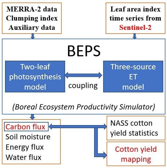
:High-resolution data with nearly global coverage from Sentinel-2 mission open a new era for crop growth monitoring and yield estimation from remote sensing. The objective of this study is to demonstrate the potential of using Sentinel-2 biophysical data combined with an ecosystem modeling approach for estimation of cotton yield in the southern United States (US). The Boreal Ecosystems Productivity Simulator (BEPS) ecosystem model was used to simulate the cotton gross primary production (GPP) over three Sentinel-2 tiles located in Mississippi, Georgia, and Texas in 2017. Leaf area index (LAI) derived from Sentinel-2 measurements and hourly meteorological data from Modern-Era Retrospective Analysis for Research and Applications, Version 2 (MERRA-2) reanalysis were used to drive the ecosystem model. The simulated GPP values at 20-m grid spacing were aggregated to the county level (17 counties in total) and compared to the cotton lint yield estimates at the county level which are available from National Agricultural Statistics Service in the United States Department of Agriculture. The results of the comparison show that the BEPS-simulated cotton GPP explains 85% of variation in cotton yield. Our study suggests that the integration of Sentinel-2 LAI time series into the ecosystem model results in reliable estimates of cotton yield.
1. Introduction
There are two major cotton types in the United States (US), one is the Pima cotton, located in the counties of Pinal and Graham in Arizona, and another type is the upland cotton (Gossypium hirsutum), a species that is native to Central America, Mexico, and the Caribbean and Gulf Coast regions, and is mainly located in southern states below 36°30′ north (N), since cotton grows well at higher temperature and in sunlight. Upland cotton is the most common type of cotton in the US, making up 95% of the planted cotton area in the US, and it is the focus of this study. Although cotton is naturally a perennial shrub, it is primarily grown as an annual crop to help pest control. In the US, the cotton is planted in spring, varying from the beginning of February to the beginning of June, and harvested in the fall. Its growing season is approximately 150 to 180 days, making it the longest of annually planted crops in the US. Since cotton is a thermophilic crop, the growing season length is important to the cotton yield. Although cotton is somewhat salt- and drought-tolerant and is an attractive crop for arid and semiarid regions, the cotton yield heavily relies on irrigation.
The cotton yield is determined by a few key factors, including species and genetics [1], soil [2] and nutrition [3,4] conditions, weather [5], irrigation [6,7], and management events [8]. Specifically, cotton is a perennial warm-season crop that requires a long growing period. Therefore, the length of growing season for cotton has a significant effect on cotton yield. For example, lint yield in double-cropping systems is significantly lower than that in monocultures [8,9].
Reliable estimation of cotton yield relies on the available information during the cotton growing season. Crop growth models, such as the Decision Support System for Agrotechnology Transfer (DSSAT) [10], are very mature in yield simulations at the plot level; however, they heavily rely on accurate inputs, such as numerous cotton traits, which are usually unavailable for large-scale applications. In contrast, remote sensing was proven as a practical approach for yield estimation at the regional and global scales [11,12,13,14,15,16,17,18]. However, the accuracy of cotton yield estimation based on remote sensing still relies on how much information is used to capture the important physiological stages during cotton development [19,20,21,22].
Using a single vegetation index [23], such as normalized difference vegetation index (NDVI), from a specific date (e.g., the maximum NDVI) can only provide limited information about cotton yield. For example, directly relating NDVI to cotton yield often gives low correlation (R2 = 0.47) [24]. Zhao et al. [25] suggested that lint yield best correlates to the canopy reflectance indices measured at the early flower stage of cotton growth (R2 of 0.56–0.89). Yang et al. [26] found that cotton yield variation (R2 = 0.52) is mostly explained by airborne hyperspectral imagery collected 9.9 weeks after planting. Inclusion of multitemporal remote sensing to capture the phenology of cotton improves the accuracy of cotton yield estimation [27,28,29,30].
Further improvement of the estimation of cotton yield requires the integration of a crop growth simulation model, remote sensing, and climate data via a data assimilation approach [31,32,33]. Essentially, remote sensing provides the biophysical parameters, e.g., leaf area index (LAI), to the crop growth model for the simulation of gross primary production (GPP), net primary production (NPP), and cotton biomass, where GPP and NPP are the indicators of crop productivity [34]. GPP is the rate at which plants capture and store atmospheric carbon dioxide to generate oxygen and energy as biomass. NPP is the difference between GPP and the energy lost during plant autotrophic respiration. NPP, thus, represents the daily accumulation of standing biomass. Since yield is related to the cumulative production of biomass during a growing season, integration of multi-source datasets achieves high accuracy in cotton yield estimation, e.g., R2 = 89% in the study of Hebbar et al. [35]. By incorporating geospatial data from remote sensing, such as LAI, into a crop growth model, Thorp et al. [36] reported that the root-mean-squared errors between measured and simulated seed cotton yield were 5% or less. In contrast to the use of complicated crop growth models, the light use efficiency (LUE) model is simple for implementation in cotton yield estimation; the LUE model can incorporate some meteorological parameters, such as temperature and vapor pressure deficit, into the yield estimation process [37], while it often lacks the capability to simulate soil water stress and the mechanism to explain the effects of CO2 fertilization (i.e., the increased rate of photosynthesis in plants that results from increased levels of carbon dioxide in the atmosphere) [38].
In addition to the improvements in modeling, the satellite images for cotton yield estimation evolved from low to high spatial resolution, e.g., Advanced Very-High-Resolution Radiometer [39], Moderate Resolution Imaging Spectroradiometer (MODIS) [40], Landsat [41], and Sentinel-2 [42]. In particular, the Sentinel-2 mission is a constellation that consists of twin satellites (Sentinel-2A and Sentinel-2B) and is operated by the European Union (EU) Copernicus Program. With these two satellites, Sentinel-2 is able to map land surface with 13 bands in the visible, near-infrared, and shortwave-infrared spectrum, a five-day revisiting time, and spatial resolutions of up to 10 m. Given its powerful capability of data collection and free, full, and open data policy, Sentinel-2 opens a new era for operational agricultural monitoring.
With only Sentinel-2A data and a 10-day revisit interval, cloud contamination is an open issue for consistently tracking the growing conditions of cotton; this challenge is similar to using only Landsat 8 for crop growth monitoring. To mitigate the cloud contamination, the available approach is to blend MODIS and Landsat for practical mapping of crop progress [43,44]. Since 2017, both Sentinel-2A and B data are available; this gives an opportunity to rely on a single data source for operational agricultural applications, as the probability of cloud contamination is reduced.
So far, the utilities of Sentinel-2A and 2B data for cotton yield mapping are still limited [42,45,46]. The objective of this study was to evaluate the potential of Sentinel-2 data as the key input to simulate cotton GPP for the purpose of yield estimation in an ecosystem model. For this aim, we collected Sentinel-2 reflectance data to derive the time series of LAI as the input of an ecosystem model; the ecosystem model integrated LAI, meteorological data, and soil data to simulate cotton GPP; the cotton GPP–yield relationship was then calibrated using yield data collected from the National Agricultural Statistics Service (NASS) in the United States Department of Agriculture (Section 2 and Section 3). The uncertainty of the GPP simulation and conclusions are summarized in Section 4 and Section 5.
2. Materials and Methods
2.1. Ecosystem Model for GPP Simulation
The Boreal Ecosystems Productivity Simulator (BEPS), hourly version, is a process-based ecosystem model to simulate water, energy, and carbon budgets [47,48,49,50,51,52]; it was used in this study to simulate cotton GPP. BEPS is in development for the last 20 years [53]. Although BEPS was initially developed for boreal ecosystems, it was expanded and used for temperate and tropical ecosystems in regional and global scales [48,51,52,54,55,56,57,58,59] and for the estimation of winter wheat yield in China [18], as C3 plants share the same photosynthesis theory at the leaf level, i.e., Farquhar’s leaf-level biochemical model [60], and BEPS has a “two-leaf” approach to upscale the ecosystem GPP to canopy level for various ecosystems including crops [49,61].
In BEPS, the canopy-level photosynthesis (GPP; ) is simulated as the sum of the total photosynthesis of sunlit and shaded leaf groups [49]:
where the subscripts “sun” and “sh” denote the sunlit and shaded components of the photosynthesis (A) and LAI (L), whereas is the stomatal resistance for carbon molecules. The sunlit and shaded LAI are separated by Equation (2) [49,61].
where is the solar zenith angle, and is the clumping index. In this study, the Sentinel-2 data were integrated into the GPP simulation through the LAI product as described in Section 2.4.
In BEPS, the vegetation biophysical and biochemical parameters are defined for plant function types including crops. For crop GPP simulation (cotton in this study), the clumping index was set to as 0.8. A detailed description of BEPS is provided in the Supplementary Materials.
2.2. Cotton-Specific Photosynthetic Parameters
Cotton leaf is characterized by a very high light saturation point (LSP). In well-watered conditions, the cotton LSP can reach 2304 µmol m−2∙s−1, and the maximum CO2 assimilation rate can reach 43.1 µmol∙m−2∙s−1 according to the experiments by Zhang et al. [62]. In photosynthesis model, Vcmax and Jmax are two important parameters to describe the photosynthetic rate at the leaf level. Vcmax is the maximum rate of carboxylation for Rubisco-limited (or light-saturated) conditions, and Jmax is the maximum rate of electron transport for the light-limited condition [60]. According to the measurements of by Harley et al. [63], cotton has a temperature optimum near 40 °C for Vcmax and 35 °C for Jmax. The Vcmax and Jmax at the optimum temperatures are four and two times higher than their respective values at 25 °C [64]; therefore, the optimum temperatures for maximum carboxylation and electron transport were set to 313.15 K and 308.15K, respectively, in BEPS. The Vcmax at 25 °C varies with leaf nitrogen and phosphorus [65,66]. Since such nutrition information is not reliably available from Sentinel-2, the cotton Vcmax at 25 °C was set to 120 µmol∙m−2∙s−1 to be consistent with our previous modeling for crops [52]. For BEPS simulation, the CO2 concentration data were obtained from https://www.esrl.noaa.gov/gmd/ccgg/trends/global.html.
2.3. Yield Estimation and Prediction
Given the total cotton GPP (g∙C∙m−2∙year−1) in the growing season simulated by BEPS, the cotton lint yield (Y, in units of kg∙ha−1) was estimated as follows:
where CUE is the carbon use efficiency or the NPP-to-GPP ratio, ranging from 0 to 1 for different species [67] and often set to 0.5 as an average of global ecosystems [68]; b is the biomass to carbon ratio; since Schlesinger [69] noted that the carbon content of biomass is almost always found to be between 45 and 50% (by oven-dry mass), b is close to 2:1; HI is the harvest index as the ratio of harvested product (grain for food crops, lint and seed for cotton) to total dry biomass (sometimes refer to the total dry aboveground biomass); this is largely determined by the percentage of bolls in the total dry biomass of cotton; l is the lint percentage of cotton (lint weight to seed cotton weight), and 10 is the ratio from g∙m−2 to kg∙ha−1.
Y = GPP × CUE × b × HI × l × 10,
The cotton HI varies with species and is affected by human management. The HI (seed cotton yield to total aboveground biomass) shown in Hussein et al. [70] was 0.34, and the lint percentage was 41%. Maheswarappa et al. [71] reported an HI of 0.3; however, the cotton HI was less than 0.1 according to the report by Pettigrew et al. [72], with a lint percentage of 41.4% on average under the rotation conditions. Huang [73] reported HI values (seed cotton to aboveground biomass) from 0.28 to 0.33. According to Dowd et al. [74], the seed-to-fiber ratio was 1.41 ± 0.11, corresponding to a lint percentage of 41% (1/2.41). Pettigrew, Bruns, and Reddy [72] reported similar lint percentages (41%). If the HI includes both seed cotton and boll trash, then l is the gin turnout ratio, which is less than the lint percentage.
Given the small variations in CUE, b, HI, and l for cotton, it is desirable to directly link GPP to yield by one coefficient C for practical application as follows:
Equation (4) assumes a linear relationship between GPP and yield; the correlation coefficient is examined below. Such a linear relationship is backed up by the strong correlation (R2 = 0.93) between biomass and seed cotton yield as measured by Huang [73]; in contrast, the LAI can only explain 51% of variance in seed cotton yield as shown in the same study. Similarly, Lambert, Traoré, Blaes, Baret, and Defourny [42] reported that the aboveground biomass explains more variation in crop yield than the peak LAI.
Once the coefficient C is derived, the yield for each pixel can be estimated with cotton GPP at the end of the growing season, and the cotton production (P) for a given region can be estimated by
where Yi is the cotton yield estimation for each pixel, A is the pixel area, and n is the number of pixels.
2.4. Sources of Model Input
The Copernicus Sentinel-2 mission comprises twin polar-orbiting satellites in the same sun-synchronous orbit, phased at 180°, aiming at monitoring land surface conditions at five-day intervals under cloud-free conditions. Each satellite carries a multispectral imager (MSI) with a swath of 290 km. The MSI provides a set of 13 spectral bands spanning from the visible and near-infrared to the shortwave-infrared, featuring four spectral bands at 10-m, six bands at 20-m, and three bands at 60-m spatial resolution. Sentinel-2A was launched on 23 June 2015 and Sentinel-2B was launched on 7 March 2017.
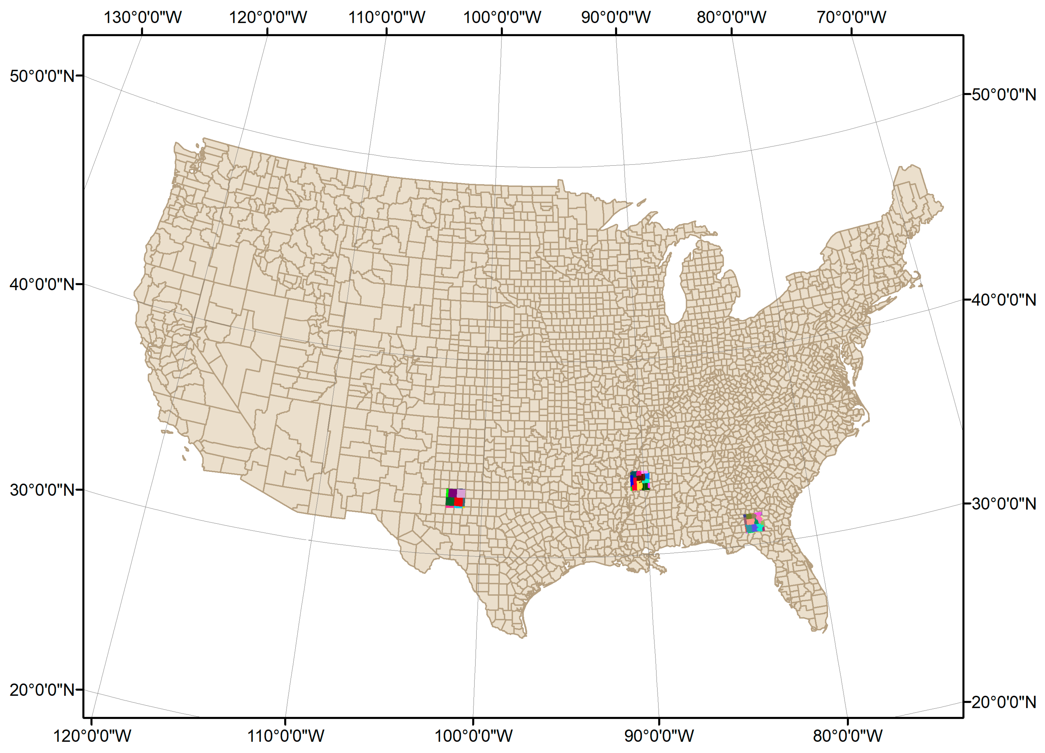
In this study, Sentinel-2 Level-1C data, top-of-atmosphere (TOA) reflectances, were used as input to the Sen2Cor atmospheric correction processor in order to convert the TOA reflectance images to the top-of-canopy (TOC) reflectance [75]. The Level-1C product results from using a digital elevation model (DEM) to project the images in cartographic geometry and is organized into tiles having an area of about 100 km2 in the Universal Transverse Mercator projection and World Geodetic System 1984 ellipsoid; the Level-1C product is available from the Copernicus Open Access Hub (https://scihub.copernicus.eu/dhus/#/home). Three tiles (14SKB, 15SYT, and 17RKQ) in 2017 were chosen in order to cover a range of high to low cotton yields in southern US as summarized in Table 1. We chose 2017 as this is the first year when both Sentinel-2A and Sentinel-2B data were available in order to minimize the contamination of cloud for cotton yield mapping; furthermore, cotton yield data for validation in 2018 were unavailable at the time when the study was conducted. The tile in Georgia (GA; 17RKQ) represents the cotton along the coastal states and a cotton yield in the middle ranges, the tile in Mississippi (MS; 15SYT) represents the cotton with better irrigation conditions and a higher yield, and the tile in Texas (TX; 14SKB) represents drier conditions and a lower cotton yield. The locations of these three tiles are shown in Figure 1.
LAI is defined as one-half of the total green leaf area per unit ground surface area (m2/m2) for broadleaf canopies [76]. It is an important structural property of vegetation. Because leaf surfaces are the common boundary for atmosphere-biosphere energy and mass exchange, important processes such as canopy interception, evapotranspiration, and gross photosynthesis are directly proportional to LAI. In BEPS, LAI is one of the most important parameters to determine the total photosynthetic rate at the canopy level. The LAI data are derived using TOC reflectance as the input to the biophysical processor available from the Sentinel Application Platform (SNAP). In SNAP, the LAI retrieval is based on an artificial neural network that relates TOC reflectances in eight bands and sun-view geometries to LAI [77]. The eight bands are B3 (560 nm), B4 (665 nm), B5 (705 nm), B6 (740 nm), B7 (783 nm), B8a (865 nm), B11 (1610 nm), and B12 (2190 nm). For the neural network training, TOC reflectances were simulated with the PROSPECT + SAIL (Scattering by Arbitrarily Inclined Leaves) model [78] corresponding to the eight Sentinel-2 bands and considering variations of primary biophysical variables related to leaf optical properties and to the canopy structure. According to Verrelst, Muñoz, Alonso, Delegido, Rivera, Camps-Valls, and Moreno [77], the uncertainty of LAI retrievals from SNAP is 0.51 m2/m2. The LAI products are derived in 20-m resolution.
Although Sentinel-2 has a high revisit frequency, the availability of cloud-free and cloud shadow-free images is limited depending on the tile location. The LAI retrievals from SNAP are often contaminated by cloud and cloud shadow; therefore, abrupt decreased LAI values are shown in the time series. To minimize the effects of cloud contamination, a locally adjusted cubic-spline capping (LACC) method was used to screen affected LAI data points and to replace them through temporal interpolation. [79]. The interpolated LAI data at the daily step were used as input to BEPS for GPP simulation.
A global reanalysis dataset, Modern-Era Retrospective Analysis for Research and Applications, Version 2 (MERRA-2), was chosen to drive BEPS simulation [80]. Six key meteorological elements including relative humidity, wind speed, and air temperature at 2 m above the surface, surface atmosphere pressure and incoming solar shortwave flux, and total precipitation at the surface level were resampled into 20-m resolution as input.
In BEPS, the soil is stratified into five layers (up to 2 m depth) for the simulation of soil water and heat fluxes. For BEPS input, four soil attributes, including texture, bulk density, organic content, and reference depth, were extracted from Soil Grids (https://soilgrids.org) [81], which provides global soil attributes at 250-m resolution.
After the cotton is harvested from the field, the raw cotton (or seed cotton) goes through the ginning processing, in order to separate the raw fiber (cotton lint) from the seeds and other debris. The raw fiber is compressed into bales. According to the Joint Cotton Industry Bale Packaging Committee (JCIBPC) in the US established in 2001, a standard cotton bale weighs 500 pounds. However, specific cotton bale weight varies between 480 and 500 pounds in different states; for example, the average bale weight in 2017 was 490 pounds (https://www.nass.usda.gov/Publications/Todays_Reports/reports/ctgnan18.pdf). For statistical purposes, NASS often reports cotton yield based on 480-pound net weight bales. In this study, we used the reported planted area (acres) and quantity of bales to calculate yield, and the bale weight was taken as 490 pounds according to the NASS statistics. The cotton yield data at the county level in 2017 from NASS were used in this study. The NASS cotton yield data are based on surveys and are the only publicly available data that cover statistics of cotton yield for all US counties.
The USDA Cropland Data Layer (CDL) product in 2017 [82,83] was used to mask out non-cotton areas for GPP simulation in the same year. The simulated cotton GPP values at 20-m resolution for each US county were averaged according to their Federal Information Processing Standard (FIPS) county code; the county-average GPP for cotton was then compared to the county-level yield data from NASS.
3. Results
3.1. Spatial Distribution of Cotton GPP in Three Sentinel-2 Tiles
One challenge to accurately simulate cotton GPP using BEPS is to determine the irrigation information. We developed an irrigation module in the GPP simulation; when this module is turned on, the soil moisture in each layer is increased to 0.42 m3/m3 (volumetric soil water content) if it is below this level every few days (e.g., 14 days). We chose 0.42 m3/m3 because this is the maximum field capacity for all soil textures [84]. In this study, there is no ideal way to identify which and when a pixel is irrigated. According to the NASS statistics, the ratios of irrigated cotton area are 32%, 34%, and 51% for Texas (TX), Georgia (GA), and Mississippi (MS), respectively; therefore, the irrigation module was turned on for tile 15SYT (MS) only.
Another challenge is to determine the start and end of growing season for cotton. In MS, the cotton is usually planted in later April or May, and the harvest begins in October and November. In the southern part of the Great Plains (covering 14SKB), the plant date can be in June. Since both cotton plots in tiles 14SKB and 15SYT are single-cropping systems, the LAI out of the growing season is low; therefore, the annual GPP is a good proxy for cotton GPP in the whole growing season. This is not true for the tile 17RKQ in GA. In the coastal plain, especially in lower south Georgia where the growing season is long, double cropping is popular. GA is characterized by a wheat–cotton cropping system, and the cotton is often planted in June; therefore, the cotton growing season for BEPS simulation was limited from June 1 to October 31.
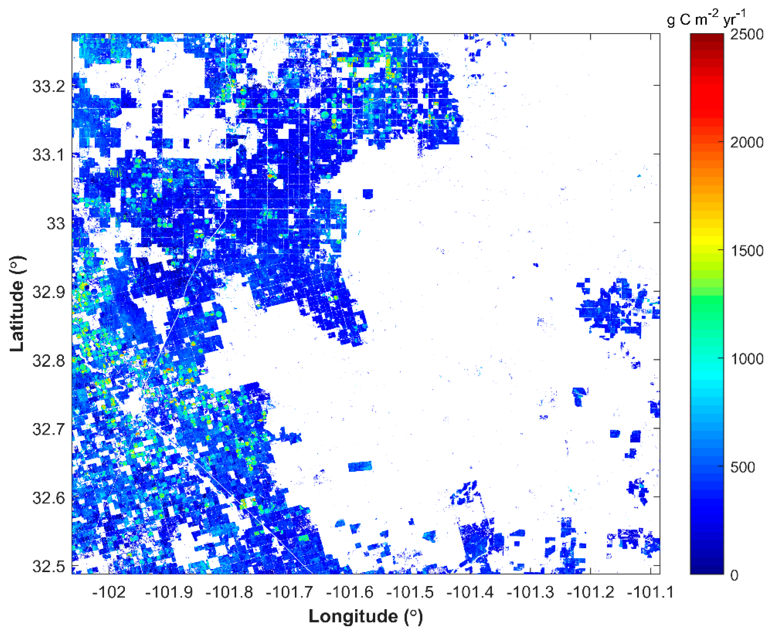
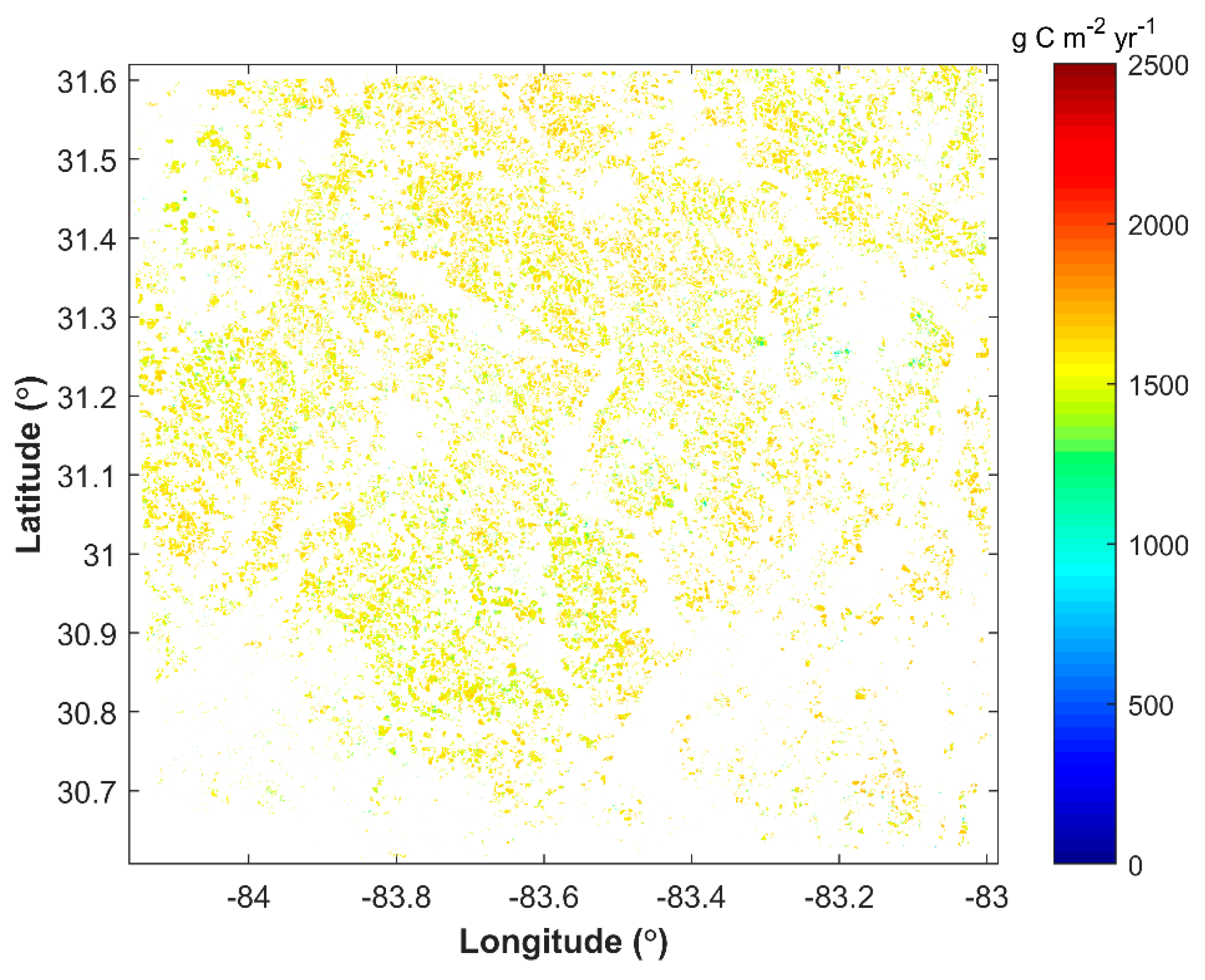
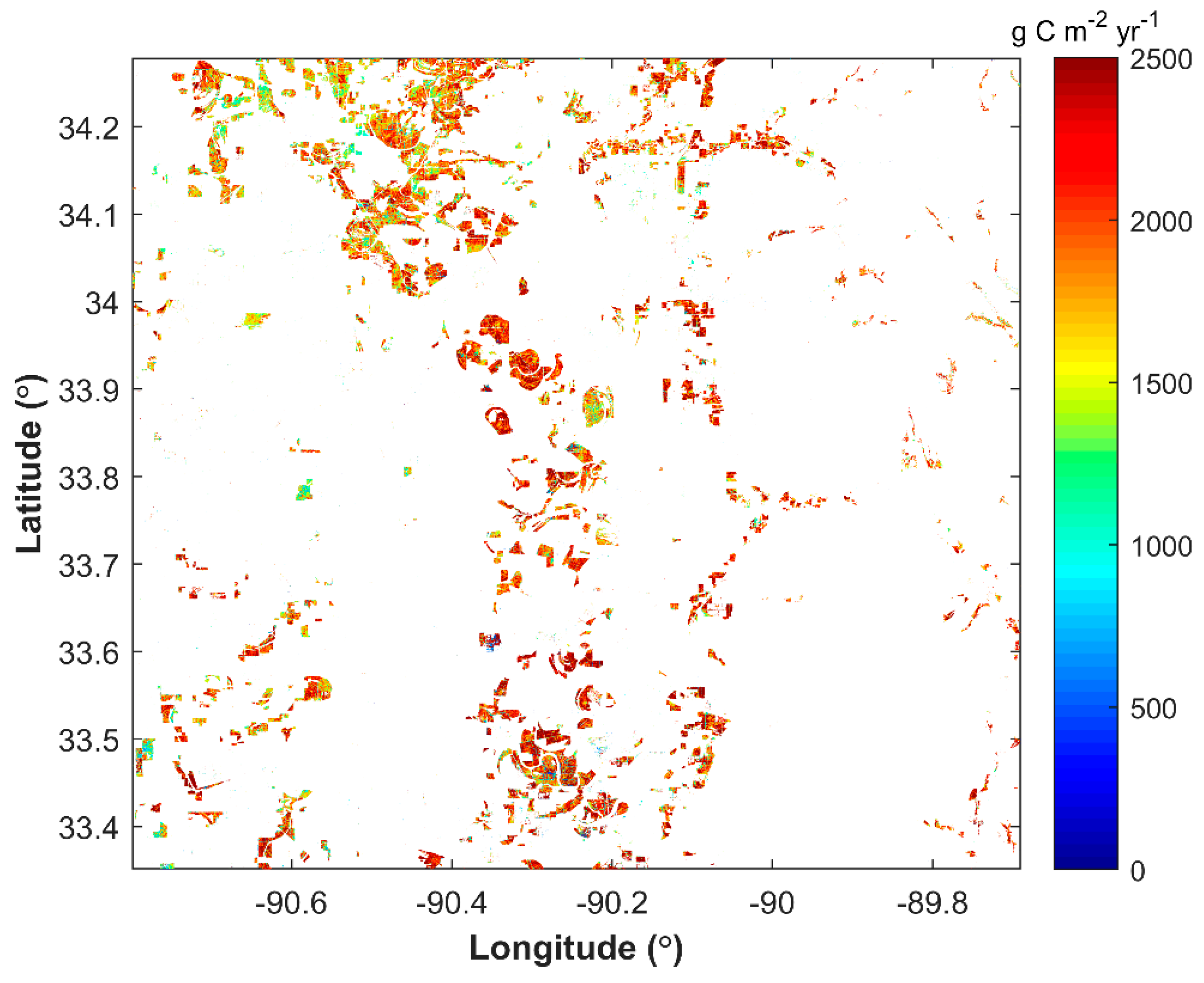
Mainly rainfed, the tile 14SKB in TX is characterized by low GPP values (726 ± 74 g∙C∙m−2∙year−1) from the BEPS simulation, although some high GPP values (~1500 g∙C∙m−2∙year−1) appear to be associated with the center-pivot irrigation (Figure 2). The GPP in the cotton growing season for tile 17RKQ is 1482 ± 74 g∙C∙m−2∙year−1 (Figure 3). Owing to the long growing season, the annual GPP for tile 15SYT is 2005 ± 177 g∙C∙m−2∙year−1 (Figure 4). The statistics of average GPP values for each county are listed in Table 2.
3.2. The GPP–Lint Yield Relationship for Upland Cotton
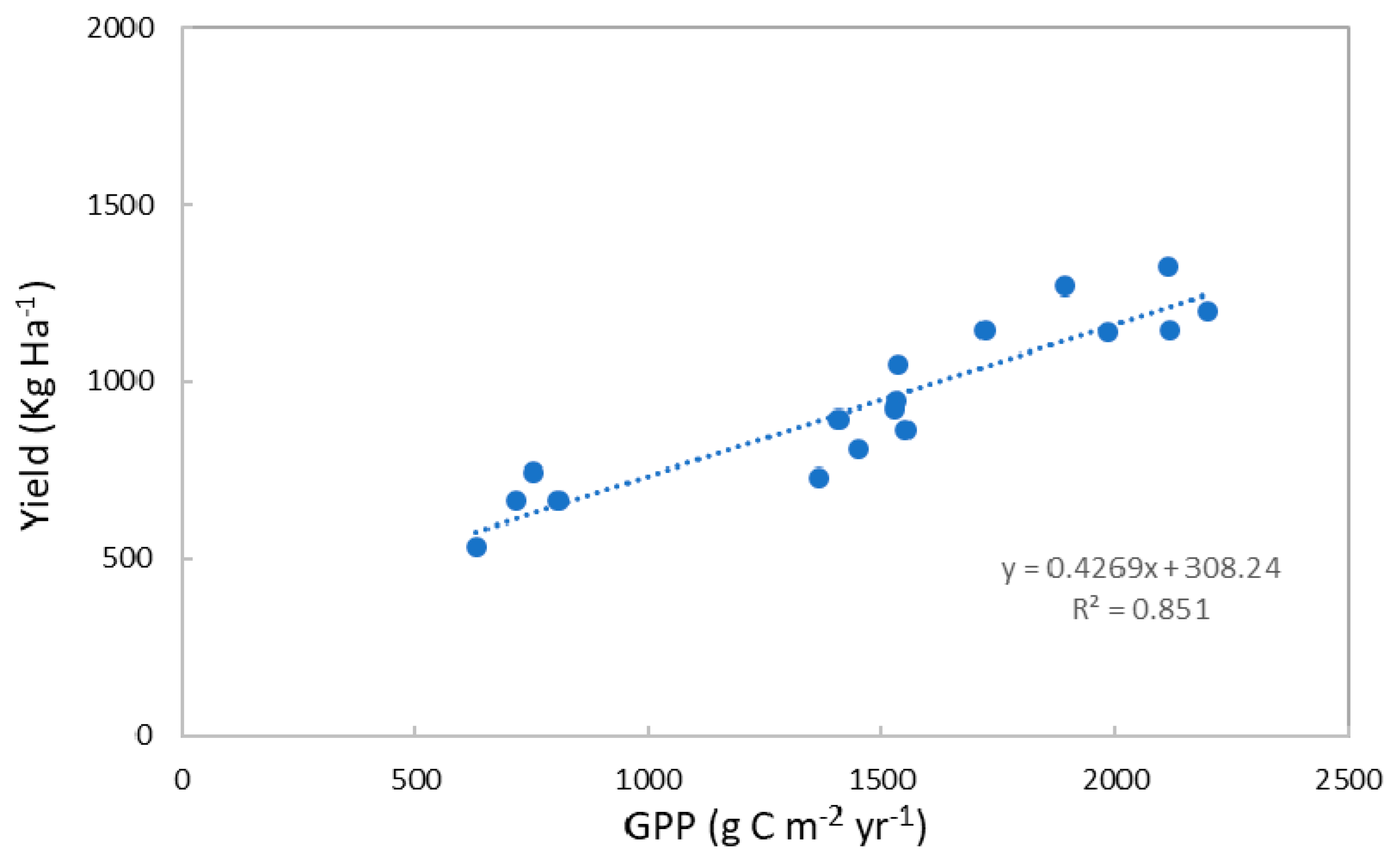
As shown in Figure 5, BEPS-simulated GPP strongly correlated with cotton lint yield from the NASS statistics for the 17 counties (R2 = 0.85). This suggests that cotton GPP from simulation can be used as a reliable proxy for cotton yield. It is noteworthy to mention that Equations (3) and (4) have no intercepts, while the regression equation in Figure 5 has an intercept. If the intercept is forced to zero in Figure 5, the slope is 0.61 and the R2 is 0.67. A similar intercept was also observed when cotton biomass was used to explain the variation in seed cotton as shown in Huang [73]. This small intercept suggests that there may be systematic uncertainty in the GPP simulation or that the correlation between GPP and cotton yield is nonlinear when both GPP and cotton yield are small. For example, the cotton Vcmax was fixed to 120 µmol∙m−2∙s−1 in our simulations as, currently, there is no such information available for each pixel from the satellite.
As shown in Table 2, the cotton lint yield in tile 17RKA (GA) was lower than the full-season cotton yield in MS. Cotton needs enough heat to grow. With respect to cotton grown in a double-crop system following wheat, the length of fruiting period and adequate temperature accumulation for boll maturation are reduced, thereby lowering the lint yield potential. Dodds et al. [85] found that, for cotton after wheat in a double-cropping system, the lint yield is generally low depending on the plant dates (lint yield range: 750–944 kg/ha). As shown in the 2012 Georgia cotton production guide (http://www.ugacotton.com/vault/productionguide/2012CottonProductionGuide.pdf), the cotton yield in a double-cropping system can have a yield reduction of up to 30% due to the limited growing season, when compared to full-season cotton planted in early May. In Arkansas, the yield potential decreases by 2% every day if cotton is planted past May 20 (https://www.uaex.edu/publications/PDF/FSA-2163.pdf). This suggests the importance of capturing planting date for cotton yield estimation, while our GPP simulation explained such variation in cotton growing season.
4. Discussions
4.1. Crop Growth Modeling
One of the core tasks for yield mapping is the modeling of crop photosynthesis. The crop growth models share in common the use of either a light use efficiency model or an enzyme kinetics-based model. For example, the modeling of cotton photosynthesis in Agricultural Production Systems Simulator (APSIM) [86] is to relate photosynthesis to radiation using an empirical equation [87]. In Crop Environment REsource Synthesis (CERES)-Wheat, the daily photosynthesis is modeled using an LUE approach [88]; the WOFOST (World Food Studies) [89] also uses Farquhar’s model [60]; the Simple Algorithm for Yield Estimation model (SAFY) also uses an LUE model for photosynthesis [90]. In common, BEPS is a process-based two-leaf enzyme kinetic ecosystem model, and the photosynthesis module of BEPS is sufficient for accurate simulation of crop photosynthesis rate. Although BEPS was initially developed for boreal ecosystems, it was expanded and used for estimations of winter wheat yield in China [18,91], for yield estimation of rapeseed in Hubei province [92], for estimation of maize yield in China [93,94], and for crop GPP modeling in Europe [95] and the US [96].
The abovementioned crop growth models have the strengths of crop trait modeling and handling of soil nutrition and water management. However, such an approach necessitates availability of these crop traits at large scales. Operational cotton yield mapping may require a compromise between large scale and high spatial resolution, and simplicity of the model structure. Similar to this work, two recent studies used Sentinel-2-derived LAI for biomass and yield mapping. Punalekar et al. [97] reported that the R2 between pasture biomass and LAI ranged from 0.16–0.73 to 0.22–0.76 for the NDVI-derived LAI and radiative transfer model-based LAI, respectively. Lambert, Traoré, Blaes, Baret, and Defourny [42] demonstrated that the R2 values between LAI and yield were 0.68, 0.62, 0.8, and 0.48 for cotton, maize, millet, and sorghum, respectively. Here, we show that the R2 value between GPP and lint yield was 0.85. Despite a single factor C in Equation (4) being used, our study demonstrates the advantage of integrating both biotic and abiotic factors for cotton yield mapping at very high spatial resolutions.
4.2. Yield Variations in Southern US Tiles
As expected, the modeled GPP did not show much variations for these tiles (14SKB and 15SYT), showing no obvious variations in cotton yield among counties either. Within tile 17RKQ, the modeled GPP explained 50% of variations in cotton yield within a narrow range. For tile 14SKB with variations in irrigation conditions (Figure 2), there were large variations in modeled GPP ranging from 500 g∙C∙m−2∙year−1 to 2500 g∙C∙m−2∙year−1, although these variations were averaged at the county level; the area with center-pivot irrigation (circles) was characterized by high GPP values up to 2500 g∙C∙m−2∙year−1. Although our study showed the important climatological effect on cotton yield, the region with highest yield was not located in GA where the condition is most ideal because of the short cotton growing season due to crop rotations; instead, the highest yield in our study was shown in MS due to their longer growing season and irrigation. This suggests that our model captured the role of crop management, in addition to the climatological effect.
5. Conclusions
In this study, we evaluated the potential of Sentinel-2A and 2B data for mapping cotton lint yield in an ecosystem model. Three Sentinel-2 tiles in southern US were chosen, covering regions with low to high cotton yields. BEPS-simulated GPP values at the pixel level were averaged into the county level and compared to the cotton lint yield data collected from NASS. Our study suggests that BEPS-simulated GPP explains 85% of variation in cotton lint yield and can be used as a reliable indicator for estimation of cotton lint yield. We also found that there may be systemic bias in our GPP simulation due to limited knowledge about cotton Vcmax, which is related to leaf nitrogen content. Accurate GPP simulation for cotton in a double-cropping system relies on the knowledge of the start and end dates of the cotton growing season, and this posed a challenge in our simulation due to certain cloud contamination in Sentinel-2 images in southern Georgia; therefore, we suggest the fusion of multi-satellite data, such as from Landsat 7 and 8, Sentinel-2, or synthetic aperture radar data from Sentinel-1 at similar spatial resolutions in order to track the key phenology stages of cotton development for a more reliable estimation of cotton yield.
Supplementary Materials
Supplementary Materials can be found at https://0-www-mdpi-com.brum.beds.ac.uk/2072-4292/11/17/2000/s1.
Author Contributions
L.H. and G.M. designed the experiment. L.H. conducted the analysis, and wrote the draft. G.M. prepared the model inputs and refined the draft. They both revised the manuscript.
Funding
This research received no external funding.
Acknowledgments
The authors thank Ting Zheng for her constructive discussion and thank Clement Atzberger for his insightful comments.
Conflicts of Interest
The authors declare no conflicts of interest.
References
- Singh, P.; Boote, K.J.; Kadiyala, M.D.M.; Nedumaran, S.; Gupta, S.K.; Srinivas, K.; Bantilan, M.C.S. An assessment of yield gains under climate change due to genetic modification of pearl millet. Sci. Total Environ. 2017, 601–602, 1226–1237. [Google Scholar] [CrossRef] [PubMed]
- Singh, K.; Mishra, S.K.; Singh, H.P.; Singh, A.; Chaudhary, O.P. Improved soil physical properties and cotton root parameters under sub-soiling enhance yield of Cotton-Wheat cropping system. Data Brief 2019, 24. [Google Scholar] [CrossRef]
- Raphael, J.P.A.; Echer, F.R.; Rosolem, C.A. Shading and nitrogen effects on cotton earliness assessed by boll yield distribution. Crop Sci. 2019, 59, 697–707. [Google Scholar] [CrossRef]
- Peng, Y.; Zhu, T.; Li, Y.; Dai, C.; Fang, S.; Gong, Y.; Wu, X.; Zhu, R.; Liu, K. Remote prediction of yield based on LAI estimation in oilseed rape under different planting methods and nitrogen fertilizer applications. Agric. For. Meteorol. 2019, 271, 116–125. [Google Scholar] [CrossRef]
- Gutierrez, A.P.; Ponti, L.; Herren, H.R.; Baumgärtner, J.; Kenmore, P.E. Deconstructing Indian cotton: Weather, yields, and suicides. Environ. Sci. Eur. 2015, 27, 12. [Google Scholar] [CrossRef]
- Masasi, B.; Taghvaeian, S.; Boman, R.; Datta, S. Impacts of irrigation termination date on cotton yield and irrigation requirement. Agriculture (Switzerland) 2019, 9, 39. [Google Scholar] [CrossRef]
- Li, P.; Ren, L. Evaluating the effects of limited irrigation on crop water productivity and reducing deep groundwater exploitation in the North China Plain using an agro-hydrological model: I. Parameter sensitivity analysis, calibration and model validation. J. Hydrol. 2019, 574, 497–516. [Google Scholar] [CrossRef]
- Du, X.; Chen, B.; Meng, Y.; Zhao, W.; Zhang, Y.; Shen, T.; Wang, Y.; Zhou, Z. Effect of cropping system on cotton biomass accumulation and yield formation in double-cropped wheat-cotton. Int. J. Plant Prod. 2015, 10, 29–44. [Google Scholar]
- Feng, L.; Wang, G.; Han, Y.; Li, Y.; Zhu, Y.; Zhou, Z.; Cao, W. Effects of planting pattern on growth and yield and economic benefits of cotton in a wheat-cotton double cropping system versus monoculture cotton. Field Crop. Res. 2017, 213, 100–108. [Google Scholar] [CrossRef]
- Jones, J.W.; Hoogenboom, G.; Porter, C.H.; Boote, K.J.; Batchelor, W.D.; Hunt, L.A.; Wilkens, P.W.; Singh, U.; Gijsman, A.J.; Ritchie, J.T. The DSSAT cropping system model. Eur. J. Agron. 2003, 18, 235–265. [Google Scholar] [CrossRef]
- Battude, M.; Al Bitar, A.; Morin, D.; Cros, J.; Huc, M.; Marais Sicre, C.; Le Dantec, V.; Demarez, V. Estimating maize biomass and yield over large areas using high spatial and temporal resolution Sentinel-2 like remote sensing data. Remote Sens. Environ. 2016, 184, 668–681. [Google Scholar] [CrossRef]
- Gao, F.; Anderson, M.; Daughtry, C.; Johnson, D. Assessing the Variability of Corn and Soybean Yields in Central Iowa Using High Spatiotemporal Resolution Multi-Satellite Imagery. Remote Sens. 2018, 10, 1489. [Google Scholar] [CrossRef]
- Habyarimana, E.; Piccard, I.; Catellani, M.; De Franceschi, P.; Dall’Agata, M. Towards Predictive Modeling of Sorghum Biomass Yields Using Fraction of Absorbed Photosynthetically Active Radiation Derived from Sentinel-2 Satellite Imagery and Supervised Machine Learning Techniques. Agronomy 2019, 9, 203. [Google Scholar] [CrossRef]
- Jin, Z.; Azzari, G.; Burke, M.; Aston, S.; Lobell, D.B. Mapping smallholder yield heterogeneity at multiple scales in eastern Africa. Remote Sens. 2017, 9, 931. [Google Scholar] [CrossRef]
- Jin, Z.; Azzari, G.; You, C.; Di Tommaso, S.; Aston, S.; Burke, M.; Lobell, D.B. Smallholder maize area and yield mapping at national scales with Google Earth Engine. Remote Sens. Environ. 2019, 228, 115–128. [Google Scholar] [CrossRef]
- Liao, C.; Wang, J.; Dong, T.; Shang, J.; Liu, J.; Song, Y. Using spatio-temporal fusion of Landsat-8 and MODIS data to derive phenology, biomass and yield estimates for corn and soybean. Sci. Total Environ. 2019, 650, 1707–1721. [Google Scholar] [CrossRef]
- Meshesha, D.T.; Abeje, M. Developing crop yield forecasting models for four major Ethiopian agricultural commodities. Remote Sens. Appl. Soc. Environ. 2018, 11, 83–93. [Google Scholar] [CrossRef]
- Wang, P.; Sun, R.; Zhang, J.; Zhou, Y.; Xie, D.; Zhu, Q. Yield estimation of winter wheat in the North China Plain using the remote-sensing-photosynthesis-yield estimation for crops (RS-P-YEC) model. Int. J. Remote Sens. 2011, 32, 6335–6348. [Google Scholar] [CrossRef]
- Huang, J.; Gómez-Dans, J.L.; Huang, H.; Ma, H.; Wu, Q.; Lewis, P.E.; Liang, S.; Chen, Z.; Xue, J.-H.; Wu, Y.; et al. Assimilation of remote sensing into crop growth models: Current status and perspectives. Agric. For. Meteorol. 2019. [Google Scholar] [CrossRef]
- Huang, J.; Ma, H.; Sedano, F.; Lewis, P.; Liang, S.; Wu, Q.; Su, W.; Zhang, X.; Zhu, D. Evaluation of regional estimates of winter wheat yield by assimilating three remotely sensed reflectance datasets into the coupled WOFOST–PROSAIL model. Eur. J. Agron. 2019, 102, 1–13. [Google Scholar] [CrossRef]
- Huang, J.; Sedano, F.; Huang, Y.; Ma, H.; Li, X.; Liang, S.; Tian, L.; Zhang, X.; Fan, J.; Wu, W. Assimilating a synthetic Kalman filter leaf area index series into the WOFOST model to improve regional winter wheat yield estimation. Agric. For. Meteorol. 2016, 216, 188–202. [Google Scholar] [CrossRef]
- Chao, Z.; Liu, N.; Zhang, P.; Ying, T.; Song, K. Estimation methods developing with remote sensing information for energy crop biomass: A comparative review. Biomass Bioenergy 2019, 414–425. [Google Scholar] [CrossRef]
- Zarco-Tejada, P.J.; Ustin, S.L.; Whiting, M.L. Temporal and spatial relationships between within-field yield variability in cotton and high-spatial hyperspectral remote sensing imagery. Agron. J. 2005, 97, 641–653. [Google Scholar] [CrossRef]
- Huang, Y.; Sui, R.; Thomson, S.J.; Fisher, D.K. Estimation of cotton yield with varied irrigation and nitrogen treatments using aerial multispectral imagery. Int. J. Agric. Biol. Eng. 2013, 6, 37–41. [Google Scholar]
- Zhao, D.; Reddy, K.R.; Kakani, V.G.; Read, J.J.; Koti, S. Canopy reflectance in cotton for growth assessment and lint yield prediction. Eur. J. Agron. 2007, 26, 335–344. [Google Scholar] [CrossRef]
- Yang, C.; Everitt, J.H.; Bradford, J.M.; Murden, D. Airborne hyperspectral imagery and yield monitor data for mapping cotton yield variability. Precis. Agric. 2004, 5, 445–461. [Google Scholar] [CrossRef]
- Meng, L.; Zhang, X.L.; Liu, H.; Guo, D.; Yan, Y.; Qin, L.; Pan, Y. Estimation of Cotton Yield Using the Reconstructed Time-Series Vegetation Index of Landsat Data. Can. J. Remote Sens. 2017, 43, 244–255. [Google Scholar] [CrossRef]
- Haghverdi, A.; Washington-Allen, R.A.; Leib, B.G. Prediction of cotton lint yield from phenology of crop indices using artificial neural networks. Comput. Electron. Agric. 2018, 152, 186–197. [Google Scholar] [CrossRef]
- Maestrini, B.; Basso, B. Predicting spatial patterns of within-field crop yield variability. Field Crop. Res. 2018, 219, 106–112. [Google Scholar] [CrossRef]
- Shi, Z.; Ruecker, G.R.; Mueller, M.; Conrad, C.; Ibragimov, N.; Lamers, J.P.A.; Martius, C.; Strunz, G.; Dech, S.; Vlek, P.L.G. Modeling of cotton yields in the Amu Darya river floodplains of Uzbekistan integrating multitemporal remote sensing and minimum field data. Agron. J. 2007, 99, 1317–1326. [Google Scholar] [CrossRef]
- Guo, C.; Tang, Y.; Lu, J.; Zhu, Y.; Cao, W.; Cheng, T.; Zhang, L.; Tian, Y. Predicting wheat productivity: Integrating time series of vegetation indices into crop modeling via sequential assimilation. Agric. For. Meteorol. 2019, 272–273, 69–80. [Google Scholar] [CrossRef]
- Kang, Y.; Özdoğan, M. Field-level crop yield mapping with Landsat using a hierarchical data assimilation approach. Remote Sens. Environ. 2019, 228, 144–163. [Google Scholar] [CrossRef]
- Meng, L.; Liu, H.; Zhang, X.; Ren, C.; Ustin, S.; Qiu, Z.; Xu, M.; Guo, D. Assessment of the effectiveness of spatiotemporal fusion of multi-source satellite images for cotton yield estimation. Comput. Electron. Agric. 2019, 162, 44–52. [Google Scholar] [CrossRef]
- Ryu, Y.; Berry, J.A.; Baldocchi, D.D. What is global photosynthesis? History, uncertainties and opportunities. Remote Sens. Environ. 2019, 223, 95–114. [Google Scholar] [CrossRef]
- Hebbar, K.B.; Venugopalan, M.V.; Seshasai, M.V.R.; Rao, K.V.; Patil, B.C.; Prakash, A.H.; Kumar, V.; Hebbar, K.R.; Jeyakumar, P.; Bandhopadhyay, K.K.; et al. Predicting cotton production using Infocrop-cotton simulation model, remote sensing and spatial agro-climatic data. Curr. Sci. 2008, 95, 1570–1579. [Google Scholar]
- Thorp, K.R.; Hunsaker, D.J.; French, A.N.; Bautista, E.; Bronson, K.F. Integrating geospatial data and cropping system simulation within a geographic information system to analyze spatial seed cotton yield, water use, and irrigation requirements. Precis. Agric. 2015, 16, 532–557. [Google Scholar] [CrossRef]
- Alganci, U.; Ozdogan, M.; Sertel, E.; Ormeci, C. Estimating maize and cotton yield in southeastern Turkey with integrated use of satellite images, meteorological data and digital photographs. Field Crop. Res. 2014, 157, 8–19. [Google Scholar] [CrossRef]
- Kirschbaum, M.U.F. Does Enhanced Photosynthesis Enhance Growth? Lessons Learned from CO2 Enrichment Studies. Plant. Physiol. 2011, 155, 117–124. [Google Scholar] [CrossRef]
- Domenikiotis, C.; Spiliotopoulos, M.; Tsiros, E.; Dalezios, N.R. Early cotton yield assessment by the use of the NOAA/AVHRR derived Vegetation Condition Index (VCI) in Greece. Int. J. Remote Sens. 2004, 25, 2807–2819. [Google Scholar] [CrossRef]
- Palacios-Orueta, A.; Huesca, M.; Whiting, M.L.; Litago, J.; Khanna, S.; Garcia, M.; Ustin, S.L. Derivation of phenological metrics by function fitting to time-series of Spectral Shape Indexes AS1 and AS2: Mapping cotton phenological stages using MODIS time series. Remote Sens. Environ. 2012, 126, 148–159. [Google Scholar] [CrossRef]
- Guo, W.; Maas, S.J.; Bronson, K.F. Relationship between cotton yield and soil electrical conductivity, topography, and Landsat imagery. Precis. Agric. 2012, 13, 678–692. [Google Scholar] [CrossRef]
- Lambert, M.J.; Traoré, P.C.S.; Blaes, X.; Baret, P.; Defourny, P. Estimating smallholder crops production at village level from Sentinel-2 time series in Mali’s cotton belt. Remote Sens. Environ. 2018, 216, 647–657. [Google Scholar] [CrossRef]
- Gao, F.; Anderson, M.C.; Zhang, X.; Yang, Z.; Alfieri, J.G.; Kustas, W.P.; Mueller, R.; Johnson, D.M.; Prueger, J.H. Toward mapping crop progress at field scales through fusion of Landsat and MODIS imagery. Remote Sens. Environ. 2017, 188, 9–25. [Google Scholar] [CrossRef] [Green Version]
- Feng, G.; Masek, J.; Schwaller, M.; Hall, F. On the blending of the Landsat and MODIS surface reflectance: Predicting daily Landsat surface reflectance. IEEE Trans. Geosci. Remote 2006, 44, 2207–2218. [Google Scholar] [CrossRef]
- Wu, M.; Yang, C.; Song, X.; Hoffmann, W.C.; Huang, W.; Niu, Z.; Wang, C.; Li, W.; Yu, B. Monitoring cotton root rot by synthetic Sentinel-2 NDVI time series using improved spatial and temporal data fusion. Sci. Rep. UK 2018, 8, 2016. [Google Scholar] [CrossRef]
- Falagas, A.; Karantzalos, K. A cotton yield estimation model based on agrometeorological and high resolution remote sensing data. Precis. Agric. 2019, 469–475. [Google Scholar] [CrossRef]
- Chen, B.Z.; Chen, J.M.; Ju, W.M. Remote sensing-based ecosystem-atmosphere simulation scheme (EASS)—Model formulation and test with multiple-year data. Ecol. Model. 2007, 209, 277–300. [Google Scholar] [CrossRef]
- Chen, J.M.; Mo, G.; Pisek, J.; Liu, J.; Deng, F.; Ishizawa, M.; Chan, D. Effects of foliage clumping on the estimation of global terrestrial gross primary productivity. Glob. Biogeochem. Cycles 2012, 26. [Google Scholar] [CrossRef]
- Chen, J.M.; Liu, J.; Cihlar, J.; Goulden, M.L. Daily canopy photosynthesis model through temporal and spatial scaling for remote sensing applications. Ecol. Model. 1999, 124, 99–119. [Google Scholar] [CrossRef] [Green Version]
- He, L.; Chen, J.M.; Liu, J.; Mo, G.; Bélair, S.; Zheng, T.; Wang, R.; Chen, B.; Croft, H.; Arain, M.A.; et al. Optimization of water uptake and photosynthetic parameters in an ecosystem model using tower flux data. Ecol. Model. 2014, 294, 94–104. [Google Scholar] [CrossRef]
- He, L.; Chen, J.M.; Liu, J.; Bélair, S.; Luo, X. Assessment of SMAP soil moisture for global simulation of gross primary production. J. Geophys. Res. Biogeosci. 2017, 122. [Google Scholar] [CrossRef]
- He, L.; Chen, J.M.; Gonsamo, A.; Luo, X.Z.; Wang, R.; Liu, Y.; Liu, R.G. Changes in the Shadow: The Shifting Role of Shaded Leaves in Global Carbon and Water Cycles Under Climate Change. Geophys. Res. Lett. 2018, 45, 5052–5061. [Google Scholar] [CrossRef] [Green Version]
- Liu, J.; Chen, J.M.; Cihlar, J.; Park, W.M. A process-based boreal ecosystem productivity simulator using remote sensing inputs. Remote Sens. Environ. 1997, 62, 158–175. [Google Scholar] [CrossRef]
- Matsushita, B.; Tamura, M. Integrating remotely sensed data with an ecosystem model to estimate net primary productivity in East Asia. Remote Sens. Environ. 2002, 81, 58–66. [Google Scholar] [CrossRef]
- Matsushita, B.; Xu, M.; Chen, J.; Kameyama, S.; Tamura, M. Estimation of regional net primary productivity (NPP) using a process-based ecosystem model: How important is the accuracy of climate data? Ecol. Model. 2004, 178, 371–388. [Google Scholar] [CrossRef]
- Feng, X.; Liu, G.; Chen, J.M.; Chen, M.; Liu, J.; Ju, W.M.; Sun, R.; Zhou, W. Net primary productivity of China’s terrestrial ecosystems from a process model driven by remote sensing. J. Environ. Manag. 2007, 85, 563–573. [Google Scholar] [CrossRef]
- Wang, Q.; Tenhunen, J.; Falge, E.; Bernhofer, C.; Granier, A.; Vesala, T. Simulation and scaling of temporal variation in gross primary production for coniferous and deciduous temperate forests. Glob. Chang. Biol 2004, 10, 37–51. [Google Scholar] [CrossRef]
- Chen, Z.; Chen, J.M.; Zhang, S.; Zheng, X.; Ju, W.; Mo, G.; Lu, X. Optimization of terrestrial ecosystem model parameters using atmospheric CO2 concentration data with the Global Carbon Assimilation System (GCAS). J. Geophys. Res. Biogeosci. 2017. [Google Scholar] [CrossRef]
- Luo, X.Z.; Chen, J.M.; Liu, J.E.; Black, T.A.; Croft, H.; Staebler, R.; He, L.M.; Arain, M.A.; Chen, B.; Mo, G.; et al. Comparison of Big-Leaf, Two-Big-Leaf, and Two-Leaf Upscaling Schemes for Evapotranspiration Estimation Using Coupled Carbon-Water Modeling. J. Geophys. Res. Biogeosci. 2018, 123, 207–225. [Google Scholar] [CrossRef]
- Farquhar, G.D.; Caemmerer, S.V.; Berry, J.A. A Biochemical-Model of Photosynthetic CO2 Assimilation in Leaves of C-3 Species. Planta 1980, 149, 78–90. [Google Scholar] [CrossRef]
- Norman, J.M. Simulation of Microclimates. In Biometeorology in Integrated Pest Management; Jerry, H., Ed.; Academic Press: Cambridge, MA, USA, 1982; pp. 65–99. [Google Scholar]
- Zhang, Y.-L.; Hu, Y.-Y.; Luo, H.-H.; Chow, W.S.; Zhang, W.-F. Two distinct strategies of cotton and soybean differing in leaf movement to perform photosynthesis under drought in the field. Funct. Plant. Biol. 2011, 38, 567–575. [Google Scholar] [CrossRef] [Green Version]
- Harley, P.C.; Thomas, R.B.; Reynolds, J.F.; Strain, B.R. Modelling photosynthesis of cotton grown in elevated CO2. Plant Cell Environ. 1992, 15, 271–282. [Google Scholar] [CrossRef]
- Leuning, R. Temperature dependence of two parameters in a photosynthesis model. Plant Cell Environ. 2002, 25, 1205–1210. [Google Scholar] [CrossRef]
- Archontoulis, S.V.; Yin, X.; Vos, J.; Danalatos, N.G.; Struik, P.C. Leaf photosynthesis and respiration of three bioenergy crops in relation to temperature and leaf nitrogen: How conserved are biochemical model parameters among crop species? J. Exp. Bot. 2011, 63, 895–911. [Google Scholar] [CrossRef]
- Singh, S.K.; Badgujar, G.B.; Reddy, V.R.; Fleisher, D.H.; Timlin, D.J. Effect of Phosphorus Nutrition on Growth and Physiology of Cotton Under Ambient and Elevated Carbon Dioxide. J. Agron. Crop Sci. 2013, 199, 436–448. [Google Scholar] [CrossRef] [Green Version]
- Zhang, Y.; Xu, M.; Chen, H.; Adams, J. Global pattern of NPP to GPP ratio derived from MODIS data: Effects of ecosystem type, geographical location and climate. Glob. Ecol. Biogeogr. 2009, 18, 280–290. [Google Scholar] [CrossRef]
- Tang, X.; Carvalhais, N.; Moura, C.; Ahrens, B.; Koirala, S.; Fan, S.; Guan, F.; Zhang, W.; Gao, S.; Magliulo, V.; et al. Global variability of carbon use efficiency in terrestrial ecosystems. Biogeosci. Discuss. 2019, 2019, 1–19. [Google Scholar] [CrossRef]
- Schlesinger, W.H. Biogeochemistry: An Analysis of Global Change; Academic Press: San Diego, CA, USA, 1991. [Google Scholar]
- Hussein, F.; Janat, M.; Yakoub, A. Assessment of yield and water use effi ciency of drip-irrigated cotton (Gossypium hirsutum L.) as aff ected by defi cit irrigation. Turk. J. Agric. For. 2011, 35, 611–621. [Google Scholar]
- Maheswarappa, H.P.; Srinivasan, V.; Lal, R. Carbon Footprint and Sustainability of Agricultural Production Systems in India. J. Crop Improv. 2011, 25, 303–322. [Google Scholar] [CrossRef]
- Pettigrew, W.T.; Bruns, H.A.; Reddy, K.N. Agronomy and Soils: Growth and Agronomic Performance of Cotton When Grown in Rotation with Soybean. J. Cotton Sic. 2016, 20, 299–308. [Google Scholar]
- Huang, J. Effects of Meteorological Parameters Created by Different Sowing Dates on Drip Irrigated Cotton Yield and Yield Components in Arid Regions in China. J. Hortic. 2015, 2, 63–83. [Google Scholar] [CrossRef]
- Dowd, M.K.; Pelitire, S.M.; Delhom, C.D. Seed-Fiber Ratio, Seed Index, and Seed Tissue and Compositional Properties of Current Cotton Cultivars. J. Cotton Sci. 2018, 22, 60–74. [Google Scholar]
- Richter, R.; Louis, J.; Müller-Wilm, U. Sentinel-2 MSI—Level 2A Products Algorithm Theoretical Basis Document. S2PAD-ATBD-0001. Eur. Space Agency (Spec. Publ.) ESA SP 2012, 49, 1–72. [Google Scholar]
- CHEN, J.M.; BLACK, T.A. Defining leaf area index for non-flat leaves. Plant Cell Environ. 1992, 15, 421–429. [Google Scholar] [CrossRef]
- Verrelst, J.; Muñoz, J.; Alonso, L.; Delegido, J.; Rivera, J.P.; Camps-Valls, G.; Moreno, J. Machine learning regression algorithms for biophysical parameter retrieval: Opportunities for Sentinel-2 and -3. Remote Sens. Environ. 2012, 118, 127–139. [Google Scholar] [CrossRef]
- Jacquemoud, S.; Verhoef, W.; Baret, F.; Bacour, C.; Zarco-Tejada, P.J.; Asner, G.P.; François, C.; Ustin, S.L. PROSPECT + SAIL models: A review of use for vegetation characterization. Remote Sens. Environ. 2009, 113, S56–S66. [Google Scholar] [CrossRef]
- Chen, J.M.; Deng, F.; Chen, M.Z. Locally adjusted cubic-spline capping for reconstructing seasonal trajectories of a satellite-derived surface parameter. IEEE Trans. Geosci. Remote 2006, 44, 2230–2238. [Google Scholar] [CrossRef]
- Rienecker, M.M.; Suarez, M.J.; Gelaro, R.; Todling, R.; Bacmeister, J.; Liu, E.; Bosilovich, M.G.; Schubert, S.D.; Takacs, L.; Kim, G.K.; et al. MERRA: NASA’s Modern-Era Retrospective Analysis for Research and Applications. J. Clim. 2011, 24, 3624–3648. [Google Scholar] [CrossRef]
- Hengl, T.; de Jesus, M.J.; Heuvelink, G.B.M.; Ruiperez Gonzalez, M.; Kilibarda, M.; Blagotić, A.; Shangguan, W.; Wright, M.N.; Geng, X.; Bauer-Marschallinger, B.; et al. SoilGrids250m: Global gridded soil information based on machine learning. Plos ONE 2017, 12, e0169748. [Google Scholar] [CrossRef]
- USDA National Agricultural Statistics Service. Cropland Data Layer; USDA-NASS: Washington, DC, USA, 2017.
- Lark, T.J.; Mueller, R.M.; Johnson, D.M.; Gibbs, H.K. Measuring land-use and land-cover change using the U.S. department of agriculture’s cropland data layer: Cautions and recommendations. Int J. Appl. Earth Obs. 2017, 62, 224–235. [Google Scholar] [CrossRef]
- Saxton, K.E.; Rawls, W.J. Soil Water Characteristic Estimates by Texture and Organic Matter for Hydrologic Solutions. Soil Sci. Soc. Am. J. 2006, 70, 1569–1578. [Google Scholar] [CrossRef] [Green Version]
- Dodds, D.M.; Dixon, T.H.; Catchot, A.L.; Golden, B.R.; Larson, E.; Varco, J.J.; Samples, C.A. Evaluation of Wheat Stubble Management and Seeding Rates for Cotton Grown Following Wheat Production. J. Cotton Sci. 2017, 21, 104–112. [Google Scholar]
- Holzworth, D.P.; Huth, N.I.; deVoil, P.G.; Zurcher, E.J.; Herrmann, N.I.; McLean, G.; Chenu, K.; van Oosterom, E.J.; Snow, V.; Murphy, C.; et al. APSIM—Evolution towards a new generation of agricultural systems simulation. Environ. Model. Softw. 2014, 62, 327–350. [Google Scholar] [CrossRef]
- Hearn, A.B. OZCOT: A simulation model for cotton crop management. Agric. Syst. 1994, 44, 257–299. [Google Scholar] [CrossRef]
- Singh, A.K.; Tripathy, R.; Chopra, U.K. Evaluation of CERES-Wheat and CropSyst models for water–nitrogen interactions in wheat crop. Agric. Water Manag. 2008, 95, 776–786. [Google Scholar] [CrossRef]
- de Wit, A.; Boogaard, H.; Fumagalli, D.; Janssen, S.; Knapen, R.; van Kraalingen, D.; Supit, I.; van der Wijngaart, R.; van Diepen, K. 25 years of the WOFOST cropping systems model. Agric. Syst. 2019, 168, 154–167. [Google Scholar] [CrossRef]
- Duchemin, B.; Maisongrande, P.; Boulet, G.; Benhadj, I. A simple algorithm for yield estimates: Evaluation for semi-arid irrigated winter wheat monitored with green leaf area index. Environ. Model. Softw. 2008, 23, 876–892. [Google Scholar] [CrossRef] [Green Version]
- Wang, P.; Xie, D.; Zhang, J.; Sun, R.; Chen, S.; Zhu, Q. Application of BEPS model in estimating winter wheat yield in North China Plain. Nongye Gongcheng Xuebao/Trans. Chin. Soc. Agric. Eng. 2009, 25, 148–153. [Google Scholar] [CrossRef]
- Ji, C.; Zhang, J.; Yao, F. The yield estimation of rapeseed in hubei province by BEPS process-based model and MODIS satellite data. Commun. Comput. Inf. Sci. 2015, 482, 643–652. [Google Scholar]
- Yao, F.; Tang, Y.; Wang, P.; Zhang, J. Estimation of maize yield by using a process-based model and remote sensing data in the Northeast China Plain. Phys. Chem. Earth 2015, 87–88, 142–152. [Google Scholar] [CrossRef]
- Yao, F.; Liu, D.; Zhang, J.; Wang, P. Estimation of Rice Yield with a Process-Based Model and Remote Sensing Data in the Middle and Lower Reaches of Yangtze River of China. J. Indian Soc. Remote Sens. 2017, 45, 477–484. [Google Scholar] [CrossRef]
- Zhang, S.; Zhang, J.; Bai, Y.; Koju, U.A.; Igbawua, T.; Chang, Q.; Zhang, D.; Yao, F. Evaluation and improvement of the daily boreal ecosystem productivity simulator in simulating gross primary productivity at 41 flux sites across Europe. Ecol. Model. 2018, 368, 205–232. [Google Scholar] [CrossRef]
- Bai, Y.; Zhang, J.; Zhang, S.; Yao, F.; Magliulo, V. A remote sensing-based two-leaf canopy conductance model: Global optimization and applications in modeling gross primary productivity and evapotranspiration of crops. Remote Sens. Environ. 2018, 215, 411–437. [Google Scholar] [CrossRef]
- Punalekar, S.M.; Verhoef, A.; Quaife, T.L.; Humphries, D.; Bermingham, L.; Reynolds, C.K. Application of Sentinel-2A data for pasture biomass monitoring using a physically based radiative transfer model. Remote Sens. Environ. 2018, 218, 207–220. [Google Scholar] [CrossRef]
Figure 1.
The locations of three Sentinel-2 tiles used in this study. Left tile: 14SKB in Texas (TX); middle tile: 15SYT in Mississippi (MS); right tile: 17RKQ in Georgia (GA). The colors highlight the location of each county.
Figure 1.
The locations of three Sentinel-2 tiles used in this study. Left tile: 14SKB in Texas (TX); middle tile: 15SYT in Mississippi (MS); right tile: 17RKQ in Georgia (GA). The colors highlight the location of each county.

Figure 2.
The simulated annual gross primary production (GPP) for cotton by the Boreal Ecosystems Productivity Simulator (BEPS) in 2017 for Sentinel-2 tile 14SKB.
Figure 2.
The simulated annual gross primary production (GPP) for cotton by the Boreal Ecosystems Productivity Simulator (BEPS) in 2017 for Sentinel-2 tile 14SKB.

Figure 3.
The simulated annual GPP for cotton by BEPS in 2017 for Sentinel-2 tile 17RKQ.

Figure 4.
The simulated annual GPP for cotton by BEPS in 2017 for Sentinel-2 tile 15SYT.

Figure 5.
The linear relationship between cotton GPP and lint yield for 17 counties in the three Sentinel-2 tiles in 2017.
Figure 5.
The linear relationship between cotton GPP and lint yield for 17 counties in the three Sentinel-2 tiles in 2017.


Table 1.
Summary of Sentinel-2 images used in this study. The three tiles cover 17 United States (US) counties in total. ID—identifier; TX—Texas; MS—Mississippi; GA—Georgia.
Table 1.
Summary of Sentinel-2 images used in this study. The three tiles cover 17 United States (US) counties in total. ID—identifier; TX—Texas; MS—Mississippi; GA—Georgia.
| Tile ID | Number of Images | Summary |
|---|---|---|
| 14SKB | 25 | TX, mainly rainfed |
| 15SYT | 16 | MS, largely irrigated |
| 17RKQ | 20 | GA, mainly rainfed |
Table 2.
The statistics of cotton area, production, and yield from the National Agricultural Statistics Service (NASS) and the Boreal Ecosystems Productivity Simulator (BEPS) in 2017 for the three Sentinel-2 tiles. FIPS—Federal Information Processing Standard; GPP—gross primary production.
Table 2.
The statistics of cotton area, production, and yield from the National Agricultural Statistics Service (NASS) and the Boreal Ecosystems Productivity Simulator (BEPS) in 2017 for the three Sentinel-2 tiles. FIPS—Federal Information Processing Standard; GPP—gross primary production.
| County | FIPS | Area | Production | Lint Yield | GPP (BEPS) |
|---|---|---|---|---|---|
| (ha) | (kg) | (kg/ha) | (g∙C∙m−2∙year−1) | ||
| TX (14SKB) | |||||
| Lynn | 48,305 | 120,522 | 79,922,356 | 663 | 715 |
| Garza | 48,169 | 16,593 | 12,322,983 | 743 | 752 |
| Dawson | 48,115 | 105,198 | 69,978,487 | 665 | 805 |
| Borden | 48,033 | 23,329 | 12,449,007 | 534 | 630 |
| MS (15SYT) | |||||
| Coahoma | 28,027 | 36,881 | 42,187,930 | 1144 | 1722 |
| Quitman | 28,119 | 10,192 | 11,590,623 | 1137 | 1985 |
| Tallahatchie | 28,135 | 17,839 | 23,602,659 | 1323 | 2116 |
| Sunflower | 28,133 | 8379 | 10,650,446 | 1271 | 1891 |
| Leflore | 28,083 | 17,748 | 21,326,898 | 1202 | 2200 |
| Carroll | 28,015 | 8859 | 10,161,688 | 1147 | 2118 |
| GA (17RKQ) | |||||
| Worth | 13,321 | 22,541 | 21,292,891 | 945 | 1532 |
| Tift | 13,277 | 9227 | 8,268,221 | 896 | 1409 |
| Colquitt | 13,071 | 19,223 | 20,181,571 | 1050 | 1536 |
| Cook | 13,075 | 7244 | 5,267,657 | 727 | 1364 |
| Berrien | 13,019 | 11,088 | 9,001,692 | 812 | 1451 |
| Thomas | 13,275 | 12,505 | 10,779,804 | 862 | 1552 |
| Brooks | 13,027 | 15,459 | 14,291,575 | 924 | 1529 |
© 2019 by the authors. Licensee MDPI, Basel, Switzerland. This article is an open access article distributed under the terms and conditions of the Creative Commons Attribution (CC BY) license (http://creativecommons.org/licenses/by/4.0/).
Share and Cite
MDPI and ACS Style
He, L.; Mostovoy, G. Cotton Yield Estimate Using Sentinel-2 Data and an Ecosystem Model over the Southern US. Remote Sens. 2019, 11, 2000. https://0-doi-org.brum.beds.ac.uk/10.3390/rs11172000
AMA Style
He L, Mostovoy G. Cotton Yield Estimate Using Sentinel-2 Data and an Ecosystem Model over the Southern US. Remote Sensing. 2019; 11(17):2000. https://0-doi-org.brum.beds.ac.uk/10.3390/rs11172000
Chicago/Turabian StyleHe, Liming, and Georgy Mostovoy. 2019. "Cotton Yield Estimate Using Sentinel-2 Data and an Ecosystem Model over the Southern US" Remote Sensing 11, no. 17: 2000. https://0-doi-org.brum.beds.ac.uk/10.3390/rs11172000
Note that from the first issue of 2016, this journal uses article numbers instead of page numbers. See further details here.