Snow Depth Estimation with GNSS-R Dual Receiver Observation


1
School of Environmental Science and Spatial Informatics, China University of Mining and Technology, Xuzhou 221116, China
2
School of Geodesy and Geomatics, Wuhan University, Wuhan 430079, China
*
Author to whom correspondence should be addressed.
Remote Sens. 2019, 11(17), 2056; https://0-doi-org.brum.beds.ac.uk/10.3390/rs11172056
Submission received: 1 July 2019
/
Revised: 25 August 2019
/
Accepted: 27 August 2019
/
Published: 1 September 2019
Abstract
:Two estimation methods using a dual GNSS (Global Navigation Satellite System) receiver system are proposed. The dual-frequency combination method combines the carrier phase observations of dual-frequency signals, whereas the single-frequency combination method combines the pseudorange and carrier phase observations of a single-frequency signal, both of which are geometry-free strictly combination and free of the effect of ionospheric delay. Theoretical models are established in the offline phase to describe the relationship between the spectral peak frequency of the combined sequence and the antenna height. A field experiment was conducted recently and the data processing results show that the root mean squared error (RMSE) of the dual-frequency combination method is 5.04 cm with GPS signals and 6.26 cm with BDS signals, which are slightly greater than the RMSE of 4.16 cm produced by the single-frequency combination method of L1 band with GPS signals. The results also demonstrate that the proposed two combination methods and the SNR method achieve similar performance. A dual receiver system enables the better use of GNSS signal carrier phase observations for snow depth estimation, achieving increased data utilization.

1. Introduction
Snow is one of the most widely geographically distributed substances on Earth’s surface and has one of the most significant seasonal and inter-annual variabilities in the cryosphere [1]. It plays a very important role in the adjustment of the global climate and hydrological cycle [2,3]. A wide range of snow abnormalities can cause atmospheric circulation anomalies. As climate change becomes more evident and climatic extremes occur more frequently, snowfall will also change greatly, which will in turn affect the cryosphere and other spheres of the Earth. Therefore, accurate information on snowfall can help to better understand the impact of snow on climate and environmental changes.
Global navigation satellite system (GNSS) not only provides the basic services of positioning, navigation, and timing, but it is also exploited to achieve other functions such as surveillance, communication, and remote sensing. GNSS remote sensing consists of two different technologies; one is GNSS radio occultation (GNSS-RO) and the other is GNSS reflectometry (GNSS-R).
GNSS-R technology was first applied to sea surface altimetry in the early 1990s [4]. Due to a number of advantages, such as low cost effectiveness and high spatial-temporal resolution, GNSS-R technology has drawn significant attention from both academia and industry. The successful launch of the United Kingdom’s TDS-1 satellite in 2014 and the eight United States’ CYGNSS (Cyclone GNSS) satellites in 2016 demonstrates the significance of this technology. Other satellite missions have also demonstrated the capabilities of GNSS-R, which includes UK-DMC (United Kingdom – Disaster Monitoring Constellation) and SMAP (Soil Moisture Active Passive) [5,6]. Over the past quarter century, the GNSS-R theoretical framework has been greatly enhanced and its application has been extended from marine remote sensing [7,8,9,10,11,12,13] to land remote sensing [14,15,16,17,18,19,20].
One of the land applications of GNSS-R technology is the measurement of snow depth. In 2009, scientists first proposed to use the signal-to-noise ratio (SNR) data recorded by continuous operating reference station (CORS) receivers to estimate snow depth, because the SNR time series contains the reflected signal component, which is associated with the snow surface height [21]. Ozeki and Heki proposed to combine the dual-frequency phase observation of the L1 carrier and the L2 carrier of GPS (Global Positioning System) signals to estimate snow depth, which is called the L4 method [22]. Yu et al. proposed a triple-frequency phase combination method that simultaneously eliminates the effects of geometry and ionospheric delay [23]. In addition, the use of GNSS-R technology for snow depth estimation has been expanded from a single GPS satellite constellation to multiple constellations, such as GLONASS (GLObal NAvigation Satellite System) [24] and BDS (BeiDou Navigation Satellite System) [25], and from a single parameter combination to a multi-parameter combination [25].
This paper introduces two combination methods, both of which consist of two steps. First, the relevant observations from the same receiver are combined to eliminate the influence of geometric distance, and then the results from two individual receivers are combined. When the signals transmitted from a satellite are simultaneously received by the dual receivers that are close to each other, the two propagation paths are approximately the same, so the combination can eliminate the influence of ionospheric delay. The combinations also eliminate or greatly weaken the effects of satellite ephemeris errors and satellite clock errors. This is because the two methods proposed in this paper use two differences, the first one is the difference between pseudorange observations and carrier phase observations of the same receiver, which can decrease the satellite clock error and ephemeris error.
2. Fundamentals of Snow Depth Estimation by GNSS-R
2.1. Signal Model with Multipath Effects
We consider the case where a typical ground GNSS receiver is used for positioning at a fixed station, such as a continuous operating reference station (CORS) in an outdoor environment. Although various techniques are developed to mitigate multipath interference, the ground reflected signal will pass through the antenna even though the amplitude is greatly reduced. When the direct signal and the reflected signal are superimposed at the receiving antenna and the receiver front end, they are simultaneously down-converted and then correlated with a replica of the pseudorandom noise code of the satellite produced by the receiver baseband digital signal processing function module, which results in multipath-induced pseudorange and carrier phase errors in GNSS measurements.
Basically, there are two different types of reflection [26]. One is the specular reflection, producing a reflected signal scattered at a single angle; the other is the diffuse reflection, resulting in multiple reflected signals scattered at many different angles, the sum of which is often modeled as an additional noise term. The specular reflection has the shortest path for the signal to reach the receiver in the ground-based observation platform when the ground surface is flat and has a power significantly greater than that of the diffuse reflection signal in the case of a flat reflection surface. Because the surface of interest is the outdoor snow surface, only the specular reflection signal is considered for the theoretical modeling and analysis for simplicity in this paper, which is simply called the reflected signal. Due to power loss caused by penetration, absorption, and propagation over a longer distance, the power of the reflected signal is significantly lower than the direct signal.
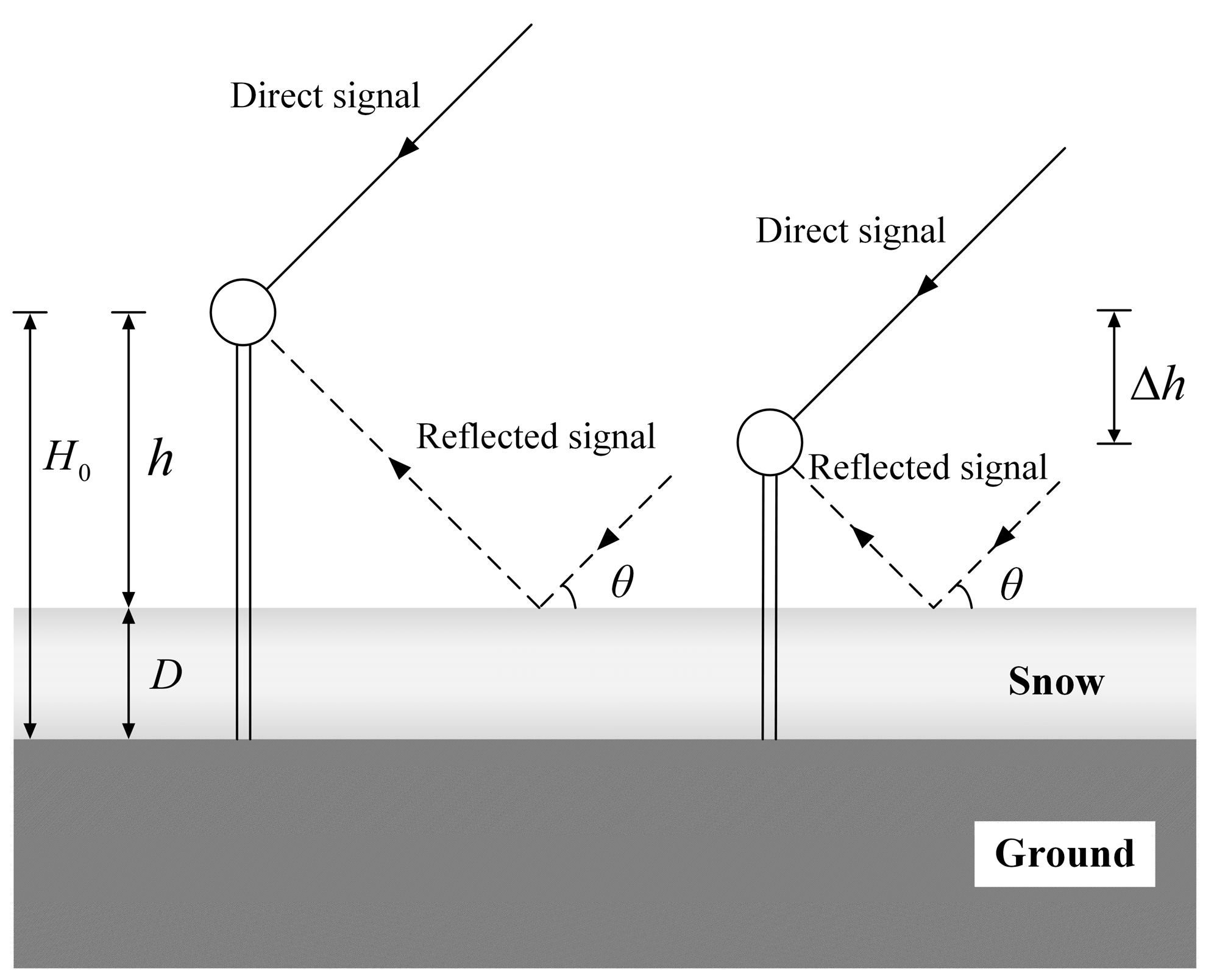
Figure 1 illustrates the dual receiver system in the presence of snow on the ground. A ground-based synchronous observation is conducted with two individual receivers separated not far away from each other. The selection of the distance between the two receivers mainly depends on the ionospheric delay. The satellite signals propagating to the two receivers should have approximately the same propagation path. Further theoretical study is needed to determine the effect of distance between the two receivers on the snow depth estimation accuracy. In the experiment to be discussed later, the distance between a pair of receivers is about 10 m. Two antennas of the same type are respectively used to capture the GNSS signal for the two receivers and there is a considerable height difference between the two antennas to form a dual receiver system. is the height of the taller antenna relative to the snow-free ground, and h is the antenna height relative to the snow surface. Snow depth D is the difference between H0 and h. Δh is the antenna height difference and θ is the satellite elevation angle.
For a single receiver, according to the geometric relationship, the reflected signal travels an extra distance compared with the direct signal, which is
Therefore, the delay time of the reflected signal relative to the direct signal is
where c is the speed of light. From (2), the interferometric phase can be readily obtained as [27]
where λ is the carrier wavelength. Only geometric delays are considered here, and phase delays caused by the antenna radiation pattern and other Fresnel reflection coefficients, such as complex values, are ignored [28].
2.2. Multipath-Induced Carrier Phase Error and Pseudorange Error
In the presence of multipath interference, the received signal is actually composed of a direct signal and a reflected signal. The pseudocode tracking loop tracks the pseudocode phase of the synthesized signal, and the difference between the tracked local pseudocode phase and the pseudocode phase of the direct signal is the multipath-induced pseudocode phase error (i.e., pseudorange error), which is [29]
where α is the amplitude ratio between the reflected and direct signal. It can be seen from (1) and (4) that the multipath-induced pseudorange error is proportional to the antenna height. Thus, to enable significant magnitude in the pseudorange error, the antenna height should be sufficient high.
The carrier tracking loop tracks the carrier phase of the synthesized signal. The difference between the tracked local carrier phase and the carrier phase of the direct signal is the multipath-induced carrier phase error, which is [23]
The modeling of the multipath-induced carrier phase error and pseudorange error greatly facilitates snow depth estimation based on GNSS-R, which is also the theoretical basis of the existing snow depth estimation methods based on carrier phase and pseudorange observations.
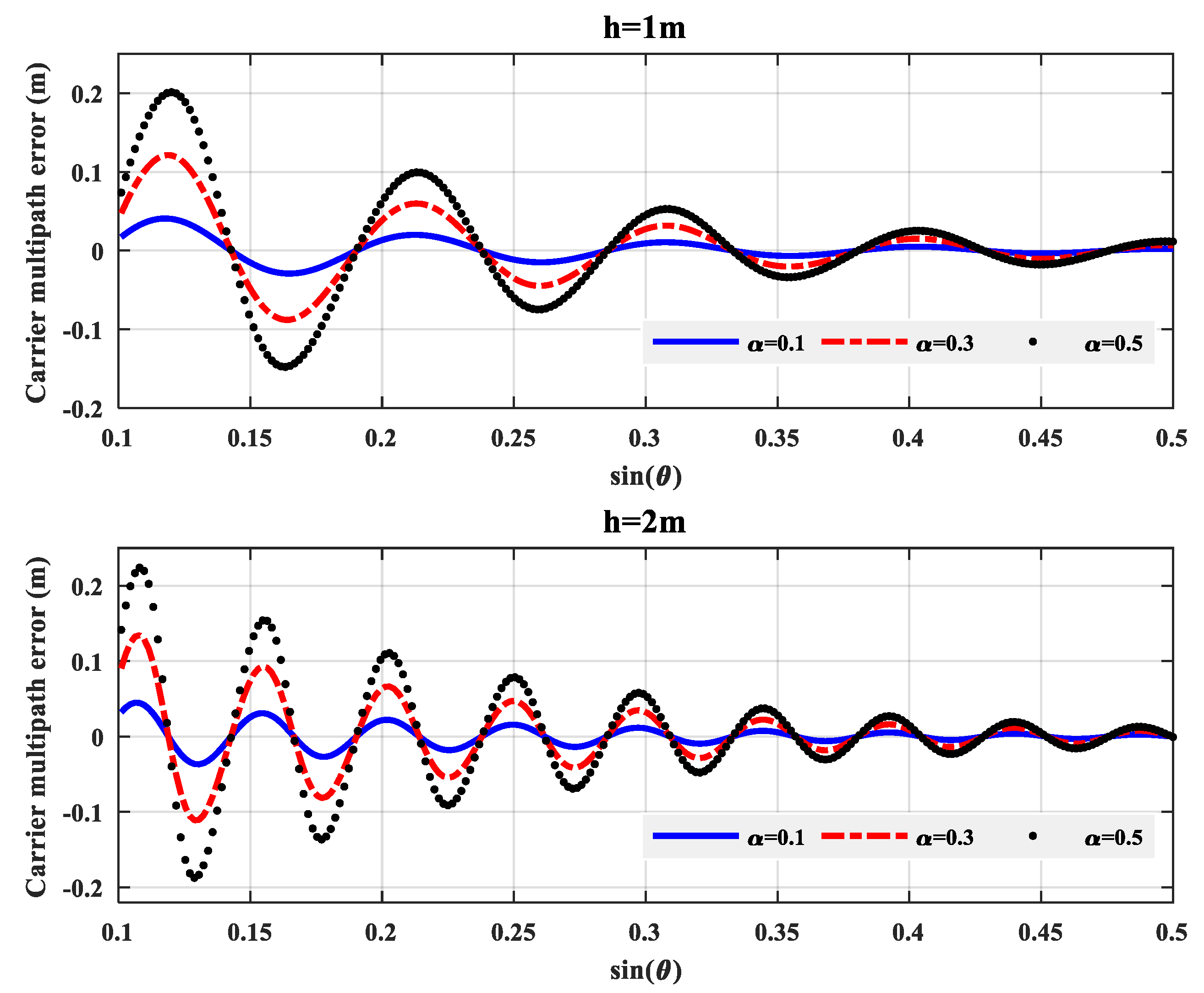
Figure 2 and Figure 3 show the variation of multipath-induced carrier phase errors and pseudorange errors with the sine of the satellite elevation angle under three different amplitude ratios, respectively. All of the oscillation curves have periodicity, and the oscillation period is the same at the same antenna height. As the relative antenna height h increases, the oscillation period becomes smaller. For a given relative antenna height h, the amplitude of the oscillation increases with α. In addition, the amplitudes of the multipath-induced errors are gradually reduced with the increase of the satellite elevation angle. This is mainly caused by the antenna radiation pattern, which usually suppresses the reflected signals more at higher elevation angles. The attenuation of the multipath-induced carrier phase error is significantly larger than the multipath-induced pseudorange error when the satellite elevation angle increase, which indicates that the observation of pseudorange errors over a longer period can be used to extract the useful information, such as the main frequency of the signal.
3. Signal Processing
3.1. The Combination Methods
Two dual-receiver based combination methods are proposed. The first one makes use of observations of two single-frequency receivers, while the second one utilizes observations of two dual-frequency receivers. For convenience, they are termed single-frequency combination (SFC) method and dual-frequency combination (DFC) method, respectively. These two methods use a similar combination procedure. That is, the combination between the observations from a single receiver is performed first, and then the combination results from the individual receivers are combined again. It is assumed that the snow depths around the two antennas are the same or the snow depth difference due to the location difference can be neglected.
The snow depth measurement system consists of GNSS satellites, two GNSS-R receivers, and two antennas. For each of the two receivers, the observation equation of the carrier phase measurement is [30]
where (unit in cycle) is the carrier phase observation multiplied by carrier wavelength; is the geometric distance between the receiver and the satellite; is the multipath-induced carrier phase error; is the receiver clock error; is satellite clock error; is the integer ambiguity; (unit in meters) is the ionospheric delay; and (unit in meters) is the tropospheric delay. Because the ionospheric delay of the pseudorange observation and that of the carrier phase are equal in value, opposite in sign, the observation equation of the pseudorange measurement is given by
where is the pseudorange observation, and l is the multipath-induced pseudorange error.
Other error sources (e.g., satellite ephemeris errors and measurement noise) are not modeled for simplicity, but they will incur an additional noise term to the final solution, if they are not removed by differential operation. The two receivers in the dual receiver system make synchronous observations and are close to each other, so that the signal propagation paths from the same satellite to the two receivers at the same time are actually the same. The ionospheric delay is a function of the signal frequency and the Total Electron Content (TEC) on the signal propagation path, so that the ionospheric delay of the same frequency is the same for both receivers under this circumstance. That is
In the SFC method, the carrier phase observations and pseudorange observations of each receiver are first combined according to
Clearly, the subtraction eliminates the geometric effect. The satellite clock error and receiver clock error are also removed by the subtraction since the pseudorange and carrier phase data are received by the same receiver and transmitted by the same satellite. The tropospheric delay is also eliminated since the propagation path associated with the pseudorange and that related to the carrier phase are exactly the same. Next, we performed a subtraction between two receivers produces
Here, is a constant during the observation period. The combination is repeatedly carried out over a consecutive number of carrier phase and pseudorange observations to generate a combination time series. Note that the combination or subtraction between the two time series in Equation (10) is with respect to the sine of the elevation angle. However, the receivers at different locations usually have different elevation angles of the same satellite. To solve this problem, the observation of one receiver with an elevation angle is combined with that of the other receiver with the most similar elevation angle. In reality, the difference between the sines of the two elevation angles would be very small. For instance, the difference between the two elevation angles considered in the processing of the data to be discussed in Section 4 is less than 0.05°. Accordingly, the difference between the sines of the two elevation angles is less than 8.73 × 10⁻⁴. The average magnitude of the difference would be close to zero. In addition, the maximum time difference between the two time-series of Equation (10) in experimental data processing is 0.5 s. Thus, the effect of the time lag on the removal of errors by differential operations would be negligible.
The DFC method uses dual frequency carrier phase observations. In the first combination, the carrier phase observations of two different frequencies of each receiver are combined as
Clearly, the geometric parameters are completely excluded due to the subtraction of two ranges. In the second combination, the first combination result of the first receiver is subtracted by that of the second receiver, yielding
Here, is a constant during the observation period.
The combinations established by the two methods are the linear combination of the multipath-induced pseudorange errors and carrier phase errors. Both multipath-induced errors are a function of carrier wavelength, relative antenna height, amplitude ratio and the sine of satellite elevation angle. The sine of satellite elevation angle is considered as an independent variable, and the amplitude ratio is empirically selected for modeling and generating theoretical results, so that different combined multipath error sequences can be obtained at different antenna height differences.
3.2. Spectral Peak Frequency Analysis
Considering that the amplitude ratio is much smaller than one due to reflection and antenna radiation pattern, Equations (4) and (5) can be approximated as
If the amplitude ratio (α) is a constant, the multipath-induced carrier phase error and pseudorange error are sinusoidal waves with frequency related to the interferometric phase and the sine of the satellite elevation angle. By treating sinθ(t) as an independent time variable, the two multipath-induced errors have a frequency given by
which is proportional to the antenna height relative to the reflection surface and inversely proportional to the carrier wavelength. However, the elevation angles vary with time and the amplitude ratio also changes with time or with the elevation angle especially due to the GNSS antenna radiation pattern which is designed to mitigate the multipath effect. As a consequence, the pseudorange and carrier phase errors are quasi-sinusoidal signals with many components of different frequencies. That is, in the frequency domain, instead of a spike at a single frequency point, a pulse-like spike with a certain bandwidth would occur. Examples of the pulse-like spike are displayed in Figure 4.
Fourier spectral analysis is commonly used to convert the time domain sequences distributed continuously and uniformly into frequency spectral sequences. Although the GNSS observation data are sampled uniformly in the time domain, such as once per second, the distribution of the sine of the satellite elevation angle is a nonlinear function of time. That is, the so-called time variable, the sine of the elevation angle, is not uniformly distributed. Therefore, Fourier transform cannot be employed for spectral analysis on the combined error signals. Instead, the Lomb Scargle method is used to perform spectrum analysis for an unevenly distributed time series [31,32].
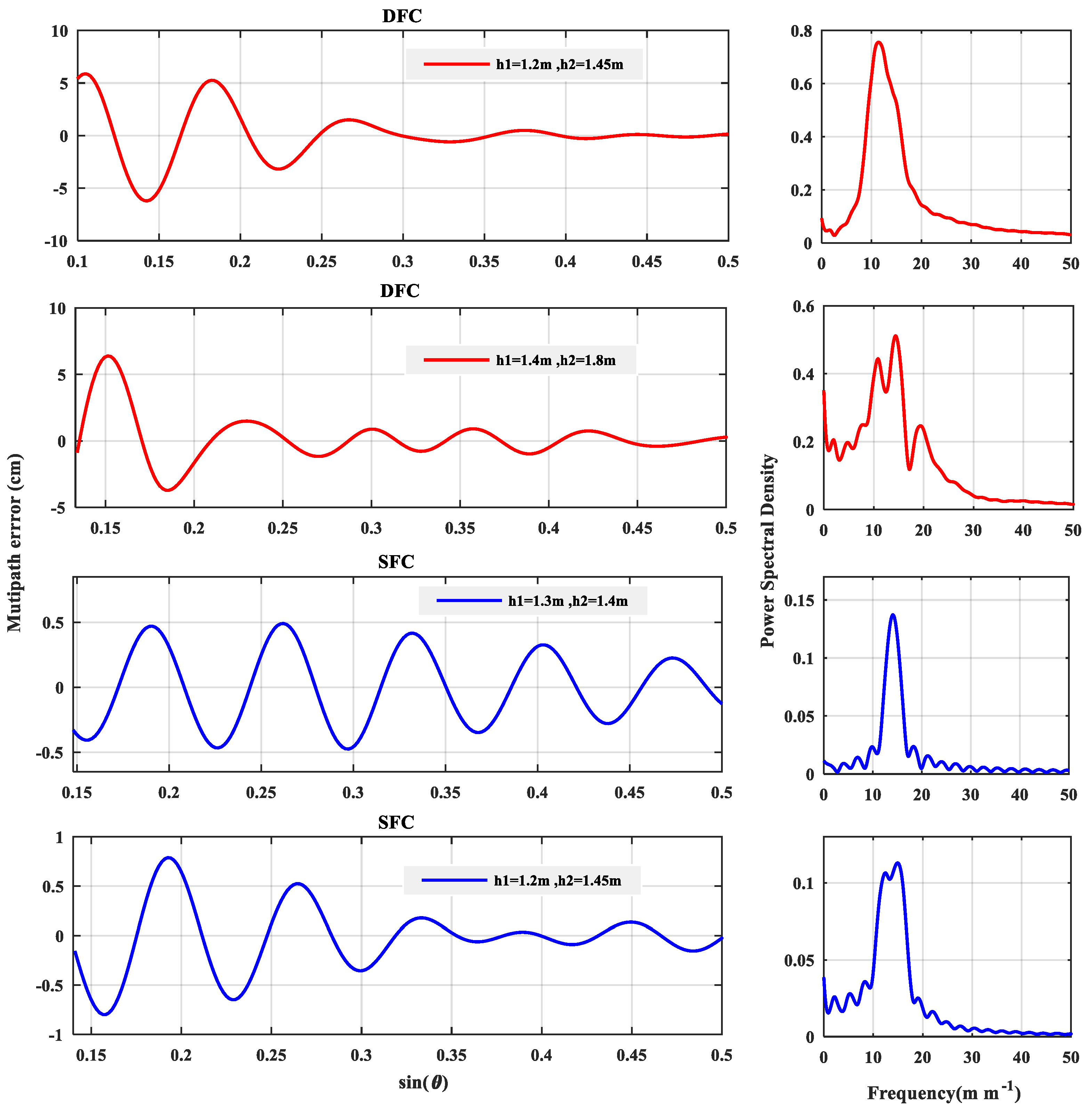
Since two receivers have two different antenna heights, the SFC method will produce signal components with two different peak frequencies. For the DFC method, there would be four different peak frequencies. Signal components of different peak frequencies will be superimposed under certain conditions. Therefore, one or two peaks will appear in the power spectrum of the SFC method, while the DFC method will have one to four peaks, depending on the two antenna heights. Figure 4 shows a few examples of the time series and power spectrum of the two combination methods.
3.3. Theoretical Model
The L-band carrier commonly used in GNSS satellites is the right-hand circularly polarized (RHCP) plane wave [33]. Due to the irregularity of the terrain and the different reflection characteristics of the surface medium, the energy of the weak signal transmitted from the satellite to the earth will be attenuated again and some signal components will be changed from the RHCP signal to the left-hand circularly polarized (LHCP) signal after being reflected by the surface. That is, the received reflected signal will consist of both RHCP and LHCP components. As the satellite elevation angle increases, the RHCP component of the reflected signal decreases and the LHCP component increases. When the ground or snow surface is flat and the reflection coefficient is a constant, the individual peak frequencies of the combined multipath-induced error are independent of the selection of satellite and satellite elevation angle range. Due to such zenith-looking placement of the continuously operating reference stations (CORS) antennas and the antenna radiation pattern, the reflected signal is stronger when the satellite elevation angle is smaller. In general, when the satellite elevation angle is in the range of 5° to 30°, better multipath information can be obtained. The combined multipath-induced error sequence is supposed to be generated over a suitable range of satellite elevation angles, and the periodogram of the multipath-induced error sequence can be obtained by Lomb Scargle spectrum analysis.
The spectral peak of the combined error time series will change from single peak to multiple peaks or vice-versa as the two antenna heights change. The inevitable ambiguity of the number of peaks brings trouble in modeling and subsequent measured data processing. In the case of a single spectral peak, it is trivial to select the peak frequency for offline modeling and online snow depth estimation. In the case of multiple spectral peaks, it is better to choose the frequency with the possible highest spectral power in the offline modeling to reduce the effect of noise. As shown in Figure 4, for instance, the spectrograms have one to three peaks. In the case of the second spectrogram, the second peak has the largest power spectral density. The corresponding peak frequency is selected for modeling. The modeling should be carried out with respect to a specific antenna and a specific signal wavelength in the case of DFC. Equation (14) can be used to find out the correspondence between the spectral peak and the antenna height and signal wavelength. Accordingly, in the online snow depth estimation, the frequency with the highest peak may be simply selected.
With Lomb Scargle spectrum analysis, the relationship between antenna height and the spectral peak frequencies of the combined error time series can be obtained by least squares fitting. Figure 5 shows the modeling case where the antenna height difference is 0.32 m. The peak frequency is positively correlated with the antenna height, hence the snow depth. Clearly, both are in good agreement with the linear model, and the simulation results of the SFC method are in better agreement with the linear model than that of the DFC method. Table 1 shows the fitting coefficients for the two different satellite constellations (GPS and BDS) and the fitting errors in terms of root mean square error (RMSE) of the linear model. For both methods, the lower antenna height (h1) above the reflection surface is assumed to be from 0.8 m to 1.5 m, and the height difference between the two antennas is 0.32 m. The selection of the antenna height difference is based on the antenna heights measured in the field experiment. The linear model can be described as
In theoretical modeling, the DFC method has an inferior fitting accuracy to the SFC method, mainly because the former produces up to four peaks superimposed and perhaps blurred in the spectrum analysis and the latter produces up to only two spectral peaks. The DFC method with BDS generates a larger fitting error. This is because when the height of the lower antenna is equal or close to 0.8 m, the points significantly deviate from the linear model. This indicates that the antenna height should be adequate to minimize the fitting error.
Assuming that the ground surface is flat and the antenna gain mode remains unchanged, the same model can be applied as long as the elevation angle range and the two antenna heights remain the same. In the measurement of snow depth, the pseudorange and carrier phase data are collected from the receiver, the data are combined according SFC or DFC to produce the error time series, the Lomb Scargle spectrum analysis is performed to obtain the spectral peak frequency of the time series, the antenna height relative to the snow surface is directly calculated by Equation (15), and finally the snow depth estimate is generated.
4. Experimental Results and Analysis
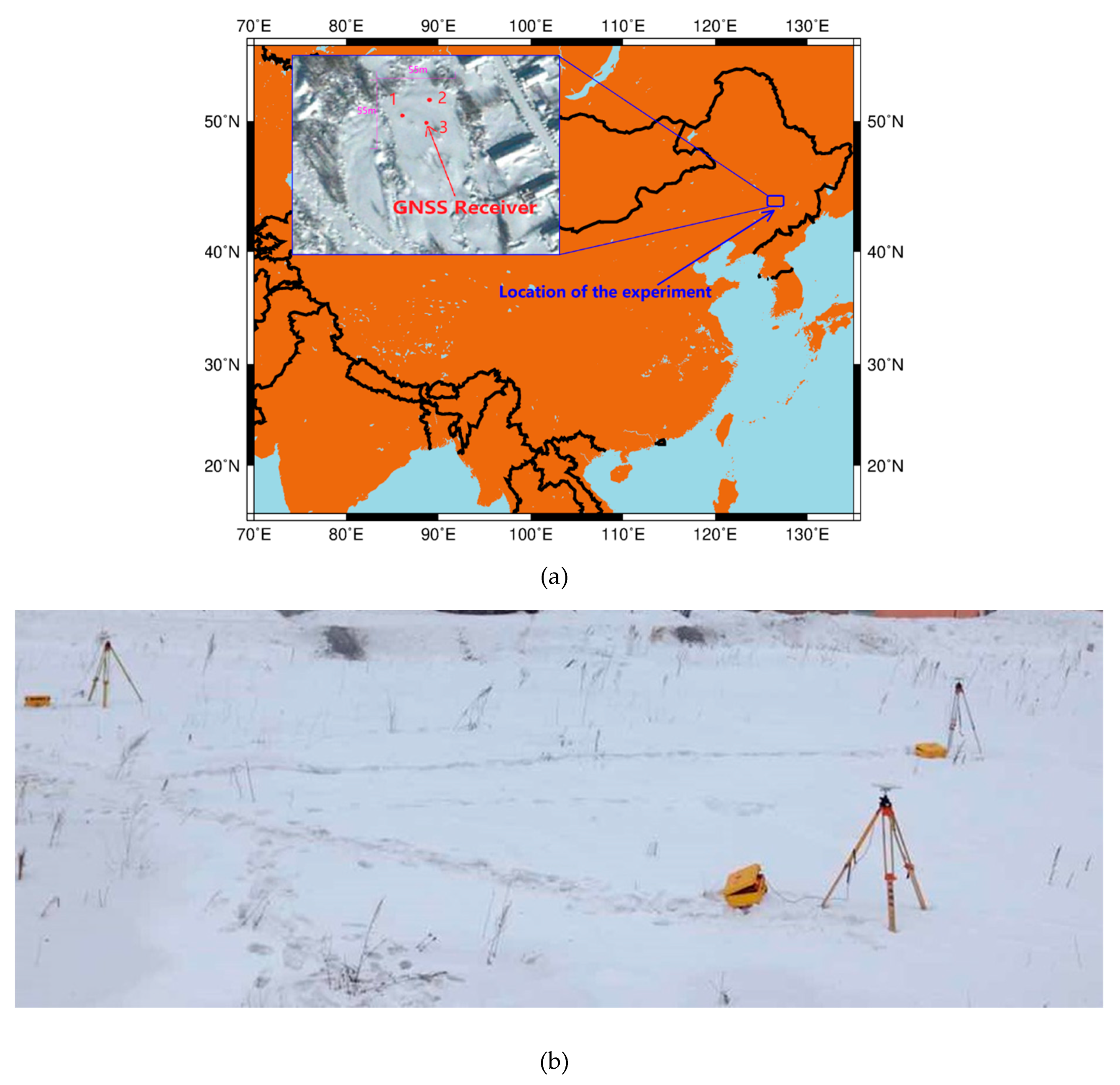
On 31 December 2016, a team from the School of Geodesy and Geomatics at Wuhan University started the experiment in a village close to Mudanjiang, Heilongjiang Province, China. The location of the experiment is shown in Figure 6a. Three receivers marked with 1, 2, and 3 were used to collect GNSS observations. The latitude and longitude of these receivers are (44.5934°,128.3986°), (44.5936°,128.3987°) and (44.5935°,128.3985°), respectively. The length and width of the experiment area are about 55 m and 55 m. As a typical climate of northeast China, snowfall occurs usually from November to March in the experimental area. The ground was covered by snow throughout the observation period. The snow depth was measured three times a day at 8:00 a.m., 11:00 a.m., and 15:00 p.m., respectively. The average snow depth in the location was between 28 cm and 60 cm during the experiment period. The increase in the snow depth was mainly caused by snowfall. As the period of the experiment was not very long, the minor decrease in the snow depth was mainly caused by wind. The snow depth changes caused by metamorphism of the snowpack were rather marginal.
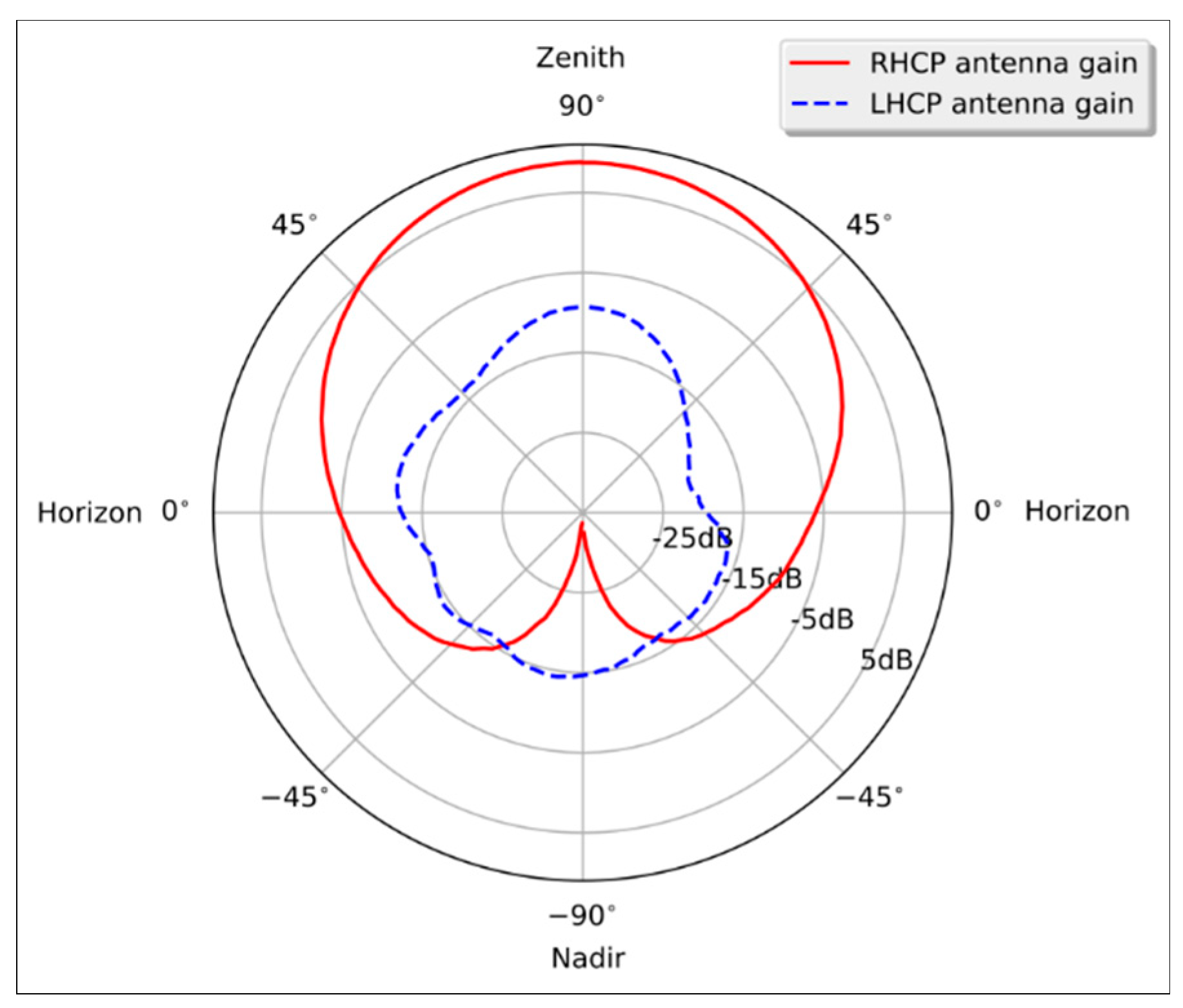
Considering the factors such as traffic and topography, a flat field adjacent to the village was selected for the experiment. Figure 6b shows the field when the ground was covered with snow. The Trimble Zephyr2 geodetic antennas were used to capture GNSS signals, adopting an advanced technology to generate a desired antenna radiation pattern to mitigate multipath effect. Figure 7 shows the typical antenna radiation pattern of a geodetic antenna. When installing, the antennas were facing up in a way similar to CORS setup. The collected GNSS signals were processed by Trimble R9 GNSS receivers, which can process signals transmitted from satellites of all four constellations (GPS, GLONASS, BDS, and Galileo).
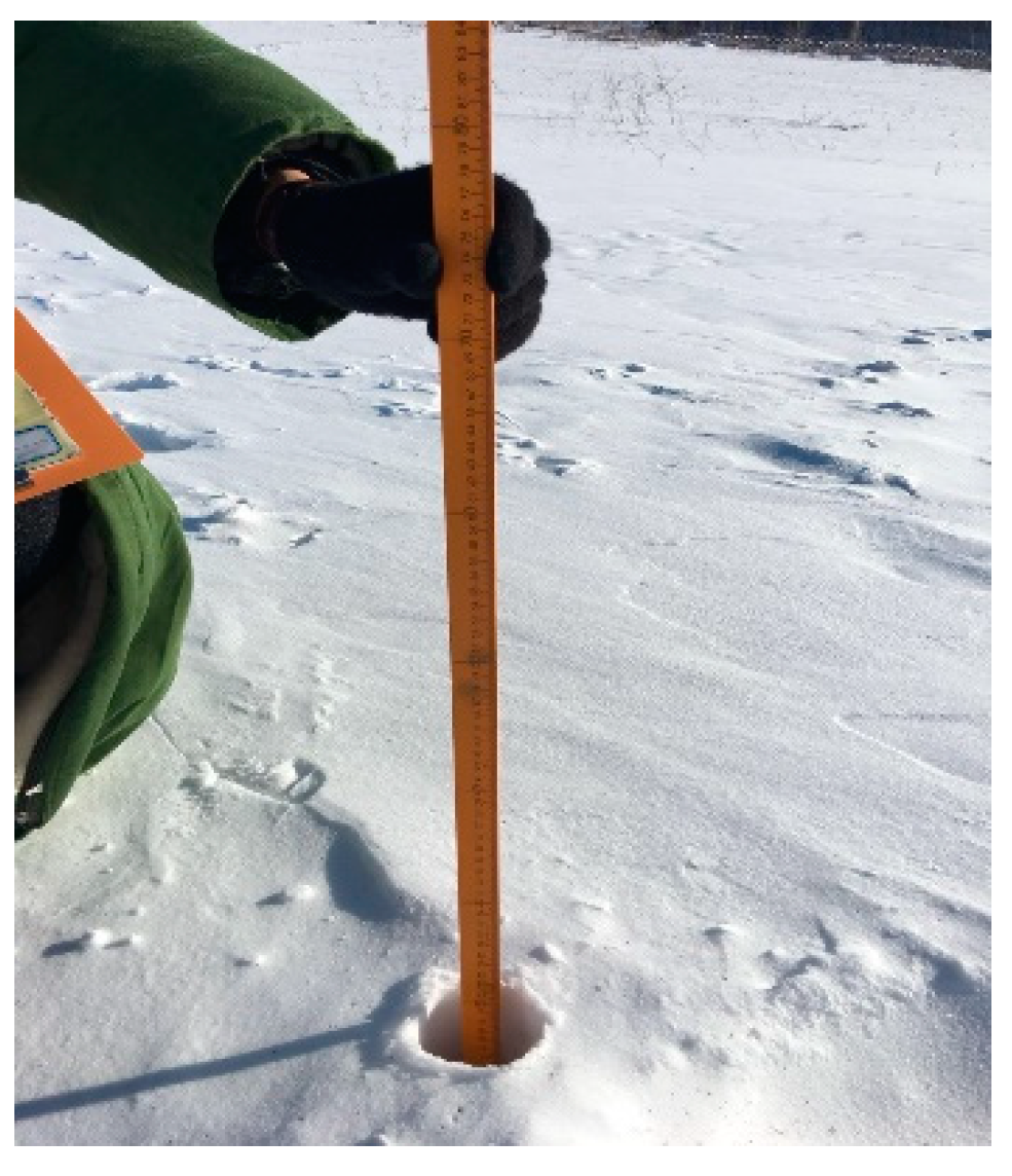
The experimental campaign was not only to estimate the snow depth, but also to estimate the snow water equivalent (SWE), although SWE estimation is not reported in this paper. The ground truth data needed to be collected and compared with the estimation result based on the GNSS-R method. An optical plummet was used to search for the snow surface point, which is on the plummet line starting from the antenna phase center point. A sampling tube of length 1m was used to dig a hole through the snow from the surface point. A steel-made tape was then used to measure the distance from a marked point on the antenna edge to the bottom of the hole, which is on the ground surface. The measured distance was used to calculate the antenna height . Since the tape was not rigid but flexible, an error in the antenna height measurement could occur. However, it has been shown that the error is typically smaller than 1 cm based on many tests. A wooden ruler was used to measure the snow depth. As shown in Figure 8, the wooden ruler was directly inserted into the hollow where the snow had been removed.
In order to obtain as many available observation data as possible, three receivers about 10 m away from each other were set for simultaneous observation, as shown in Figure 6. Table 2 shows the GNSS satellite signals of the pseudorange and carrier phase which were used to estimate snow depth. The antenna height was from 0.8 m to 1.6 m, and the antenna height difference ranged from 9.43 cm to 40.56 cm. The experiment campaign was conducted over 12 consecutive days. The GNSS antennas remained fixed, while the receiver batteries were taken away for recharging after eight-hour observation each day.
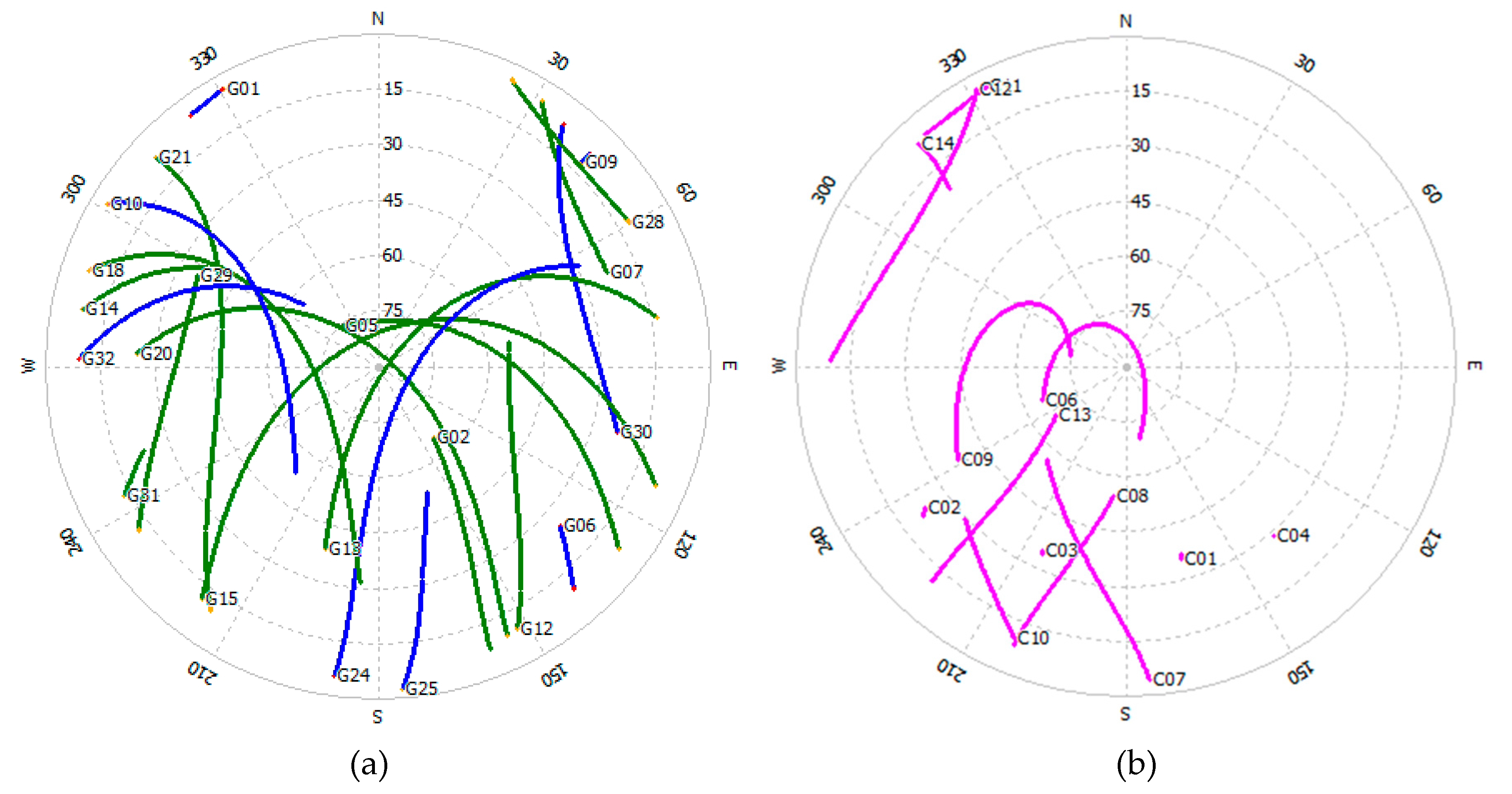
Figure 9 shows the skyplots of GPS and BDS satellites observed at one of the receivers over an interval of about eight hours on 2 January 2017. Clearly, the number of visible GPS satellites is much larger than that of BDS satellites.
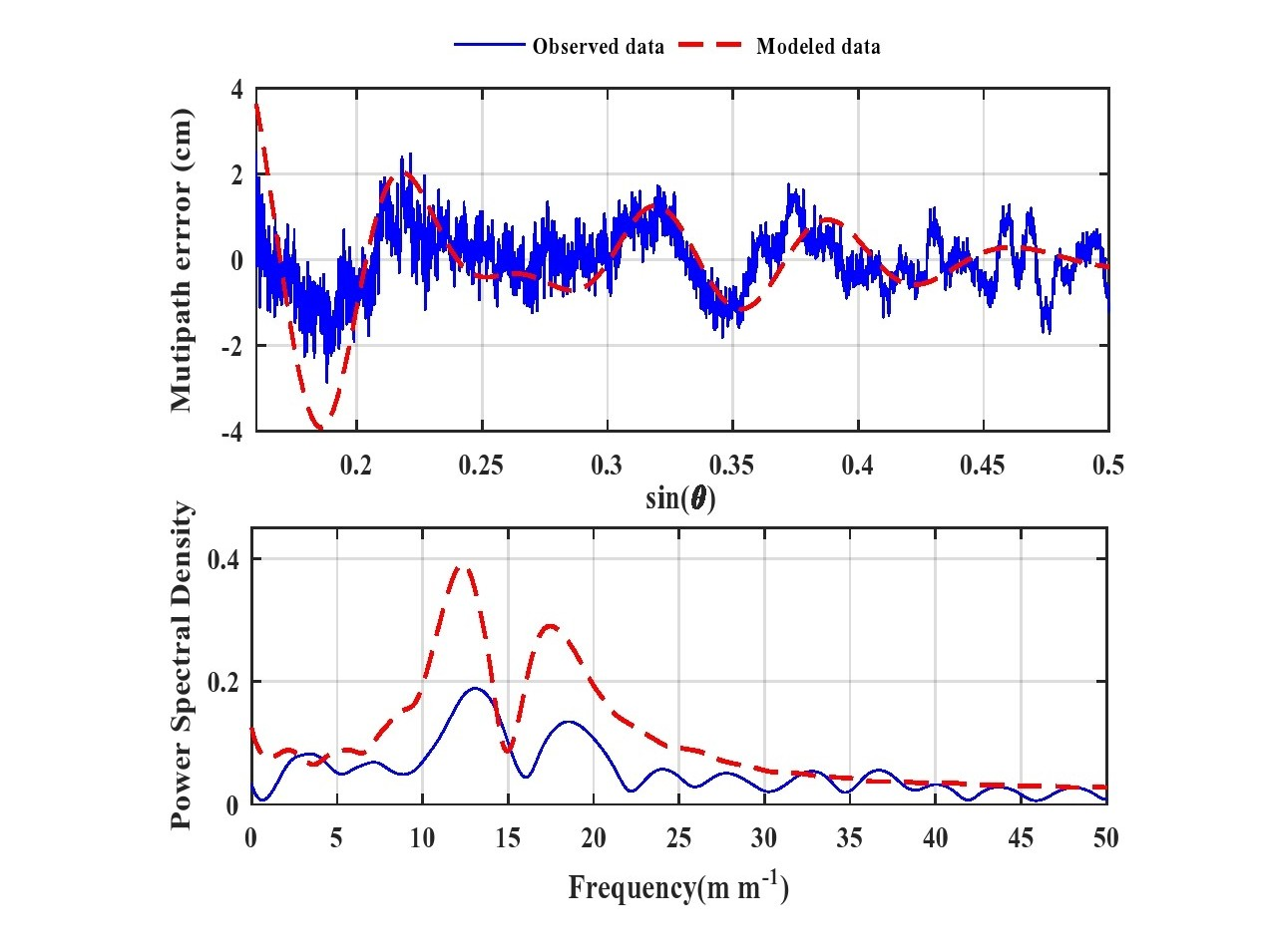
Figure 10 shows a typical example of a multipath-induced time series produced by DFC method and its power spectral density. Results from both the modeling and experiment are presented. Clearly, the time series generated from experimental data shows a clear oscillating pattern, which has a good match with the modeled time series. Although the power spectrum patterns of the modelled time series and the observed one are very similar in terms of the two spikes, the spectral power of the observed data is significantly lower than the modelled one due to noise. Furthermore, the two spectral peak frequencies of the observed data slightly deviate from those of modelled data due to noise corruption.
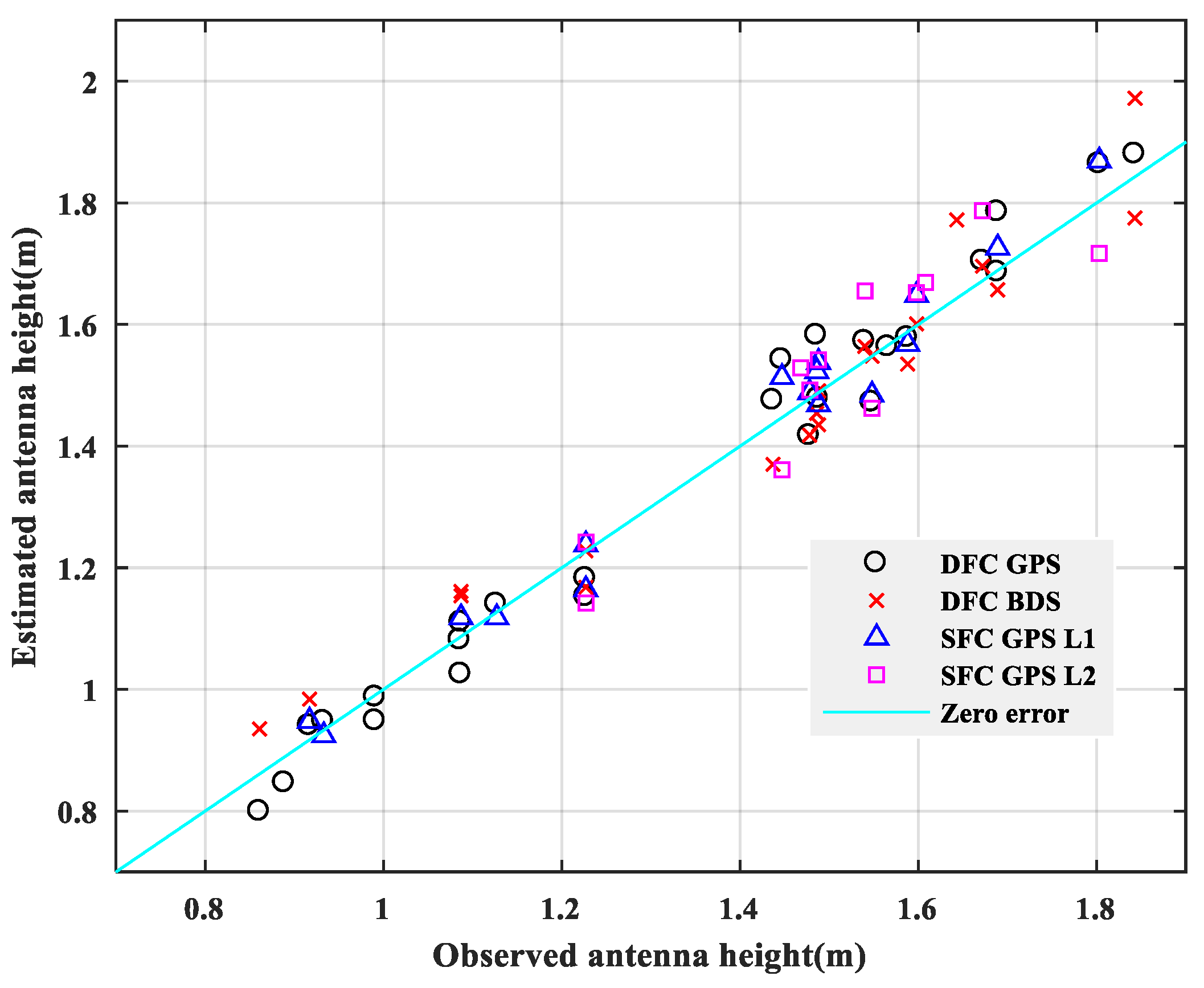
The observation data collected by two receivers with fixed antenna height difference in the same satellite system were processed to obtain the observation antenna heights corresponding to the estimated antenna heights under the two estimation methods. Figure 11 shows the comparison between the estimated antenna heights of the two combination methods with different satellite systems and the true antenna heights. The straight line represents the zero-error line.
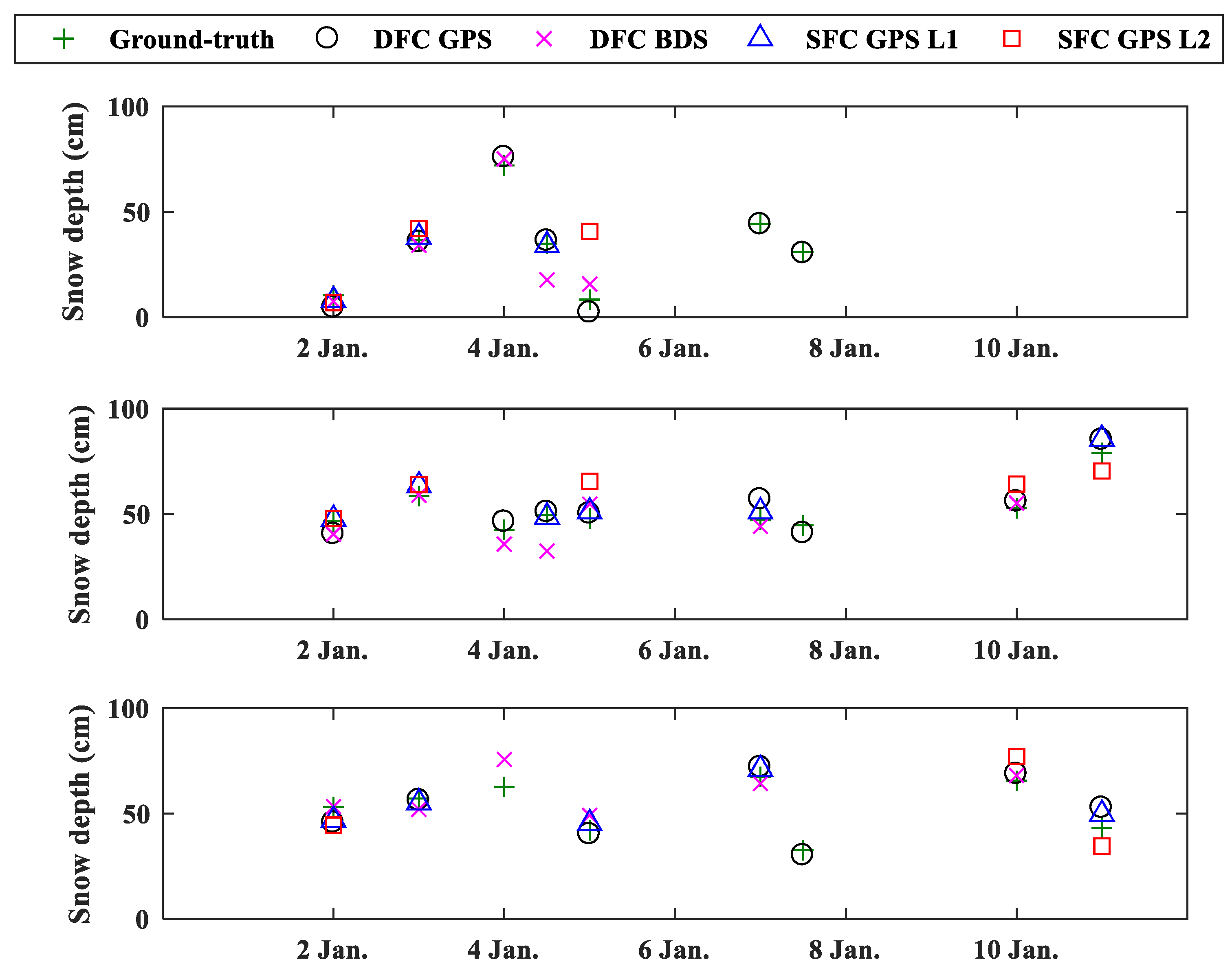
Figure 12 shows the daily snow depth observed (i.e., ground truth) and estimated results associated with three receivers. In general, there is good agreement between the ground truth and all estimates using the two combination methods under different satellite systems. It can be seen that the estimation results with GPS signals are generally better than the estimation results with BDS signals, probably because the BDS pseudorange observation data contains stronger noise under this circumstance. The SFC method of the L1 band was superior to the DFC method with the same satellite system, whereas the SFC method of the L2 band had different characteristics, which showed the worst estimation result. The main reason could be that the SFC method was considerably less affected by the superposition of multiple spectral peaks, and the theoretical modeling of DFC method was less accurate than the SFC method. However, the SFC method was more sensitive to data quality, and pseudorange observations of the L1 band contained larger noise than that of the L2 band.
Table 3 also confirms this conclusion from a statistical point of view, which shows the mean error, error standard deviation (STD), and RMSE of the snow depth estimation for three methods (i.e., SNR method [23], DFC method, and SFC method) with the two different satellite systems. The SFC method of the L1 band slightly outperformed the SNR method. Both combination methods with GPS observation data tended to have an underestimation of the actual antenna height, resulting in the overestimation of the snow depth. BDS observations produced opposite results to GPS observations, which underestimated the snow depth. The penetration of the signal and inner reflection beneath the snow surface could also bring estimation errors. The observation area was not perfectly flat, and there were some dried grasses on the floor mixed with the snow, producing additional errors.
In addition, when the snow depth suddenly increases or decreases, due to wind, an additional estimation error will be produced. Such a wind-caused variation would depend on the wind speed and direction as well as its duration. Furthermore, strict simultaneous observations are not guaranteed between the two receivers, making the effects of geometry and ionospheric delays incompletely eliminated. These factors may also contribute to the snow depth estimation error.
5. Conclusions
This paper proposed two new methods for estimating snow depth using a dual GNSS receiver system. One uses observations of dual-frequency carrier phases, and the other uses observations of single-frequency carrier phases and pseudorange. Both methods can eliminate the influence of geometric distance and the influence of ionospheric delay. The snow depth is indirectly obtained by establishing a theoretical model between the peak frequency and the antenna height. The theoretical model relies on the satellite elevation angle and antenna gain pattern. For given two antenna heights, the snow depth estimate can be obtained using the same model, which greatly simplifies the data processing. The estimation accuracy of the proposed two methods is affected by the superposition of peaks for some relative antenna heights above snow surface, and the DFC method suffers a greater impact. It is significant to select the heights and height difference of two antennas, so as to minimize such impact. The SFC method has different estimation results in different bands. The L2 band contains larger noise, which makes its estimation accuracy lower. By comparison, the estimation accuracy of the SNR method is better than the DFC method, and the estimation accuracy of the SFC method of the L1 band is the best.
Future research will focus on mitigating the effect of noise, such as by data fusion of signals of different frequencies and different satellites, to improve the estimation accuracy and look into the selection of the distance between two receivers as well as the selection of the heights of two antennas. In addition, SWE is a more useful index to measure snowfall, and SWE estimation will be an ongoing research issue.
Author Contributions
Y.L. and X.C. designed and performed the experiment and made initial processing of the data; J.L. helped to organize the experiment and to obtain the equipment for the experiment, and provided supervision; S.W. analyzed the data, wrote the initial version of the paper, and validated the new combination methods; K.Y. conceived the new combination methods, organized the experiment, wrote the revised version of the paper, and provided supervision.
Funding
This research was funded by the National Natural Science Foundation of China under Grants 41574031 and 41730109, Advanced Research Projects of the 13th Five-Year Plan of Civil Aerospace Technology, Key Laboratory of Geospace Environment and Geodesy, Ministry of Education, Wuhan University under Grant 17-02-07 and Jiangsu Dual Creative Teams Programme Project awarded in 2017 (Grant ID CUMT07180005).
Acknowledgments
The authors would like to thank senior engineer Zhonghai Zhao at the Heilongjiang No.1 Mapping Engineering Institute for his help with the experiment.
Conflicts of Interest
The authors declare no conflict of interest.
References
- Armstrong, R.L.; Brun, E. Snow and climate: Physical processes, surface energy exchange and modeling. Polar Res. 2010, 29, 461–462. [Google Scholar]
- Qian, Y.; Gustafson, W.I.; Leung, L.R.; Ghan, S.J. Effects of soot-induced snow albedo change on snowpack and hydrological cycle in western United States based on Weather Research and Forecasting chemistry and regional climate simulations. J. Geophys. Res. Atmos. 2009, 114. [Google Scholar] [CrossRef] [Green Version]
- Qian, Y.; Flanner, M.G.; Leung, L.; Wang, W. Impacts of Tibetan Plateau snowpack pollution on the Asian hydrological cycle and monsoon climate. Atmos. Chem. Phys. 2010, 10. [Google Scholar] [CrossRef]
- Martin-Neira, M. A passive reflectometry and interferometry system (Paris): Application to ocean altimetry. ESA J. 1993, 17, 331–355. [Google Scholar]
- Gleason, S.; Hodgard, S.; Sun, Y.; Gommenginger, C.; Mackin, S.; Adjrad, M.; Unwin, M. Detection and processing of bistatically reflected GPS signals from a low Earth orbit for the purpose of ocean remote sensing. IEEE Trans. Geosci. Remote Sens. 2005, 43, 1229–1241. [Google Scholar] [CrossRef]
- Carreno-Luengo, H.; Lowe, S.T.; Zuffada, C.; Esterhuizen, S.; Oveisgharan, S. Spaceborne GNSS-R from the SMAP mission; first assessment of polarimetric scatterometry over land and cryosphere. Remote Sens. 2017, 9, 362. [Google Scholar] [CrossRef]
- Auber, J.C.; Bilbaut, A.; Rigal, L. Characterization of Multipath on Land and Sea at GPS Frequencies. In Proceedings of the ION-GPS-94 Conference, Paris, France, 20–23 September 1994; pp. 1155–1171. [Google Scholar]
- Anderson, K.D. A GPS tide gauge. GPS World Showcase 1995, 6, 44. [Google Scholar]
- Katzberg, S.J.; Garrison, J.J.L. Utilizing GPS to Determine Ionospheric Delay Over the Ocean; NASA Langley Technical Report Server: Hampton, Virginia, USA, December 1996. [Google Scholar]
- Zavorotny, V.U.; Voronovich, A.G. Scattering of GPS signals from the ocean with wind remote sensing application. IEEE Trans. Geosci. Remote Sens. 2000, 38, 951–964. [Google Scholar] [CrossRef] [Green Version]
- Fabra, F.; Cardellach, E.; Rius, A.; Ribo, S.; Oliveras, S.; Nogues-Correig, O.; Rivas, M.B.; Semmling, M.; D’Addio, S. Phase altimetry with dual polarization GNSS-R over sea ice. IEEE Trans. Geosci. Remote Sens. 2012, 50, 2112–2121. [Google Scholar] [CrossRef]
- Welk, B.; Kodama, R. Detection of a Sea Surface Salinity Gradient Using Data Sets of Airborne Synthetic Aperture Radiometer HUT-2-D and a GNSS-R Instrument. IEEE Trans. Geosci. Remote Sens. 2011, 49, 4561–4571. [Google Scholar]
- Valencia, E.; Camps, A.; Rodriguez-Alvarez, N.; Park, H.; Ramos-Perez, I. Using GNSS-R Imaging of the Ocean Surface for Oil Slick Detection. IEEE J. Sel. Topics Appl. Earth Observ. 2013, 6, 217–223. [Google Scholar] [CrossRef]
- Masters, D.; Axelrad, P.; Katzberg, S. Initial results of land-reflected GPS bistatic radar measurements in SMEX02. Remote Sens. Environ. 2004, 92, 507–520. [Google Scholar] [CrossRef]
- Egido, A.; Paloscia, S.; Motte, E.; Guerriero, L.; Pierdicca, N.; Caparrini, M.; Santi, E.; Fontanelli, G.; Floury, N. Airborne GNSS-R Polarimetric Measurements for Soil Moisture and Above-Ground Biomass Estimation. IEEE J. Sel. Topics Appl. Earth Observ. 2014, 7, 1522–1532. [Google Scholar] [CrossRef]
- Rodriguez-Alvarez, N.; Camps, A.; Vall-llossera, M.; Bosch-Lluis, X.; Monerris, A.; Ramos-Perez, I.; Valencia, E.; Marchan-Hernandez, J.F.; Martinez-Fernandez, J.; Baroncini-Turricchia, G.; et al. Land Geophysical Parameters Retrieval Using the Interference Pattern GNSS-R Technique. IEEE Trans. Geosci. Remote Sens. 2010, 49, 71–84. [Google Scholar] [CrossRef]
- Rodriguez-Alvarez, N.; Bosch-Lluis, X.; Camps, A.; Ramos-Perez, I.; Valencia, E.; Park, H.; Vall-llossera, M. Vegetation Water Content Estimation Using GNSS Measurements. IEEE Trans. Geosci. Remote Sens. 2012, 9, 282–286. [Google Scholar] [CrossRef]
- Gamba, M.T.; Marucco, G.; Pini, M.; Ugazio, S.; Falletti, E.; Lo Presti, L. Prototyping a GNSS-Based Passive Radar for UAVs: An Instrument to Classify the Water Content Feature of Lands. Sensors 2015, 15, 28287–28313. [Google Scholar] [CrossRef] [PubMed]
- Larson, K.M. A new way to detect volcanic plumes. Geophys. Res. Lett. 2013, 40, 2657–2660. [Google Scholar] [CrossRef]
- Ferrazzoli, P.; Guerriero, L.; Pierdicca, N.; Rahmoune, R. Forest biomass monitoring with GNSS-R: Theoretical simulations. Adv. Space Res. 2011, 47, 1823–1832. [Google Scholar] [CrossRef]
- Larson, K.M.; Gutmann, E.E.; Zavorotny, V.U.; Braun, J.J.; Williams, M.W.; Nievinski, F.G. Can we measure snow depth with GPS receivers? Geophys. Res. Lett. 2009, 21, 876–880. [Google Scholar] [CrossRef]
- Ozeki, M.; Heki, K. GPS snow depth meter with geometry-free linear combinations of carrier phases. J. Geod. 2012, 86, 209–219. [Google Scholar] [CrossRef]
- Yu, K.; Ban, W.; Zhang, X.; Yu, X. Snow depth estimation based on multipath phase combination of GPS triple-frequency signals. IEEE Geosci. Remote Sens. Lett. 2015, 53, 5100–5109. [Google Scholar] [CrossRef]
- Qian, X.; Jin, S. Estimation of Snow Depth from GLONASS SNR and Phase-Based Multipath Reflectometry. IEEE J. Sel. Top. Appl. Earth Observ. 2016, 9, 4817–4823. [Google Scholar] [CrossRef]
- Yu, K.; Li, Y.; Xin, C. Snow Depth Estimation Based on Combination of Pseudorange and Carrier Phase of GNSS Dual-Frequency Signals. IEEE Trans. Geosci. Remote Sens. 2019, 57, 1817–1828. [Google Scholar] [CrossRef]
- Hinrikus, H. Electromagnetic Waves; Wiley Encyclopedia of Biomedical Engineering: Hoboken, New Jersey, 2006. [Google Scholar]
- Bilich, A.; Larson, K.M. Mapping the gps multipath environment using the signal-to-noise ratio (SNR). Radio Sci. 2007, 42, 1–16. [Google Scholar] [CrossRef]
- Nievinski, F.G.; Larson, K.M. Forward modeling of GPS multipath for near-surface reflectometry and positioning applications. GPS Solut. 2014, 18, 309–322. [Google Scholar] [CrossRef]
- Axelrad, P.; Larson, K.; Jones, B. Use of the correct satellite repeat period to characterize and reduce site-specific multipath errors. In Proceedings of the 18th Intnational Technical Meeting Satellite Division Institute Navigation (ION GNSS), Long Beach, CA, USA, 13–16 September 2005; pp. 2638–2648. [Google Scholar]
- Enge, P.K. The Global Positioning System: Signals, measurements, and performance. Int. J. Wirel. Inf. Netw. 1994, 1, 83–105. [Google Scholar] [CrossRef]
- Lomb, N.R. Least-squares frequency analysis of unequally spaced data. Astrophys. Space Sci. 1976, 39, 447–462. [Google Scholar] [CrossRef]
- Scargle, J.D. Studies in astronomical time series analysis. II—Statistical aspects of spectral analysis of unevenly spaced data. Astrophys. J. 1982, 263, 835–853. [Google Scholar] [CrossRef]
- Hofmann-Wellenhof, B.; Lichtenegger, H.; Wasle, E. GNSS—Global Navigation Satellite Systems: GPS, GLONASS Galileo and More; Springer: New York, NY, USA, 2008. [Google Scholar]
Figure 1.
The dual receiver system for snow depth estimation.

Figure 2.
Considering the actual antenna radiation pattern, the multipath-induced carrier phase error of GPS L1 band signals vary with the sine of the satellite elevation angle when the antenna height is 1 m (top) and 2 m (bottom).
Figure 2.
Considering the actual antenna radiation pattern, the multipath-induced carrier phase error of GPS L1 band signals vary with the sine of the satellite elevation angle when the antenna height is 1 m (top) and 2 m (bottom).

Figure 3.
Considering the actual antenna radiation pattern, the multipath-induced pseudorange phase error of GPS L1 band signals vary with the sine of the satellite elevation angle when the antenna height is 1 m (top) and 2 m (bottom).
Figure 3.
Considering the actual antenna radiation pattern, the multipath-induced pseudorange phase error of GPS L1 band signals vary with the sine of the satellite elevation angle when the antenna height is 1 m (top) and 2 m (bottom).

Figure 4.
The variation of combined sequence with the sine of the satellite elevation angle and spectrograms under different antenna heights.
Figure 4.
The variation of combined sequence with the sine of the satellite elevation angle and spectrograms under different antenna heights.

Figure 5.
Linear relationship between the lower antenna height and spectral peak frequency by least squares fitting using GPS observation, when the antenna height difference is 0.32 m.
Figure 5.
Linear relationship between the lower antenna height and spectral peak frequency by least squares fitting using GPS observation, when the antenna height difference is 0.32 m.

Figure 6.
(a) Location of the experiment; (b) three receivers for GNSS data collection are not far away from each other.
Figure 6.
(a) Location of the experiment; (b) three receivers for GNSS data collection are not far away from each other.

Figure 7.
Example of radiation patterns of a typical geodetic GNSS antenna.

Figure 8.
A wooden ruler for measuring snow depth.

Figure 9.
The skyplots of different satellite constellations on 2 January 2017. (a) The skyplot of GPS satellites. (b) the skyplot of BDS satellites.
Figure 9.
The skyplots of different satellite constellations on 2 January 2017. (a) The skyplot of GPS satellites. (b) the skyplot of BDS satellites.

Figure 10.
Time series and power spectral density produced by DFC method with simulated data (dashed red line) and observed data (solid blue line) of the GPS G18 when the heights of the two antennas are 1.486 m and 1.689 m, respectively.
Figure 10.
Time series and power spectral density produced by DFC method with simulated data (dashed red line) and observed data (solid blue line) of the GPS G18 when the heights of the two antennas are 1.486 m and 1.689 m, respectively.

Figure 11.
Observed (ground-truth) antenna heights versus estimated antenna heights obtained by the proposed methods with GPS and BDS observation data.
Figure 11.
Observed (ground-truth) antenna heights versus estimated antenna heights obtained by the proposed methods with GPS and BDS observation data.

Figure 12.
The three scatter plots show the daily snow depth observed and estimated results for GPS and BDS by two proposed methods. The three subplots are produced using models generated with the three antennas of the three receivers, respectively.
Figure 12.
The three scatter plots show the daily snow depth observed and estimated results for GPS and BDS by two proposed methods. The three subplots are produced using models generated with the three antennas of the three receivers, respectively.


Table 1.
Fitting coefficients for GPS and BDS.
| Method | GNSS | Antenna | a (m−1) | b (m) | RMSE (cm) |
|---|---|---|---|---|---|
| DFC | GPS | h1 | 0.0991 | −0.0021 | 0.70 |
| h2 | 0.0991 | 0.3179 | |||
| BDS | h1 | 0.0961 | 0.0363 | 1.16 | |
| h2 | 0.0961 | 0.3563 | |||
| SFC | GPS | h1 | 0.0932 | −0.3030 | 0.47 |
| h2 | 0.0932 | 0.0170 |
Table 2.
GNSS observation codes for GPS and BDS.
| GNSS System | Band | Signals | |
|---|---|---|---|
| Pseudorange | Carrier Phase | ||
| GPS | L1 | C1C | L1C |
| L2 | — | L2W | |
| BDS | B1 | C2I | L2I |
| B2 | — | L7I | |
Table 3.
Mean error, STD, and RMSE of different methods.
| Method | GNSS | Band | Mean (cm) | STD (cm) | RMSE (cm) |
|---|---|---|---|---|---|
| SNR | GPS | L1 | 0.84 | 4.23 | 4.31 |
| L2 | 0.92 | 4.36 | 4.46 | ||
| DFC | GPS | L1, L2 | −0.21 | 5.04 | 5.04 |
| BDS | L1, L2 | 0.02 | 6.26 | 6.26 | |
| SFC | GPS | L1 | −1.28 | 3.96 | 4.16 |
| L2 | −1.22 | 7.54 | 7.64 |
© 2019 by the authors. Licensee MDPI, Basel, Switzerland. This article is an open access article distributed under the terms and conditions of the Creative Commons Attribution (CC BY) license (http://creativecommons.org/licenses/by/4.0/).
Share and Cite
MDPI and ACS Style
Yu, K.; Wang, S.; Li, Y.; Chang, X.; Li, J. Snow Depth Estimation with GNSS-R Dual Receiver Observation. Remote Sens. 2019, 11, 2056. https://0-doi-org.brum.beds.ac.uk/10.3390/rs11172056
AMA Style
Yu K, Wang S, Li Y, Chang X, Li J. Snow Depth Estimation with GNSS-R Dual Receiver Observation. Remote Sensing. 2019; 11(17):2056. https://0-doi-org.brum.beds.ac.uk/10.3390/rs11172056
Chicago/Turabian StyleYu, Kegen, Shuyao Wang, Yunwei Li, Xin Chang, and Jiancheng Li. 2019. "Snow Depth Estimation with GNSS-R Dual Receiver Observation" Remote Sensing 11, no. 17: 2056. https://0-doi-org.brum.beds.ac.uk/10.3390/rs11172056
Note that from the first issue of 2016, this journal uses article numbers instead of page numbers. See further details here.