Analysis of Ship Detection Performance with Full-, Compact- and Dual-Polarimetric SAR

Abstract

Polarimetric synthetic aperture radar (SAR) is currently drawing more attention due to its advantage in Earth observations, especially in ship detection. In order to establish a reliable feature selection method for marine vessel monitoring purposes, forty features are extracted via polarimetric decomposition in the full-polarimetric (FP), compact-polarimetric (CP), and dual-polarimetric (DP) modes. These features were comprehensively quantified and evaluated using the Euclidean distance and mutual information, and the result indicated that the features in CP SAR are better than those of FP or DP SAR in general. The CP SAR features are thus further studied, and a new feature, named phase factor, in CP SAR mode is presented that can distinguish ships and the sea surface by the constant 0 without complex calculation. Furthermore, the phase factor is independent of the sea surface roughness, and hence it performs stably for ship detection even in high sea states. Experiments demonstrated that the ship detection performance of the phase factor detector is better than that of roundness, delta, HESA and CFAR detectors in low, medium and high sea states.

1. Introduction

Ship detection is of great significance in maritime traffic, immigration control, and fishing activity monitoring. Synthetic aperture radar (SAR) can work day and night with high resolution, even under cloudy conditions, and has been widely used in ship detection.

Constant false alarm rate (CFAR) detection is a classic method and has been used extensively and effectively in SAR images for ship target detection. The key to the CFAR method is the selection of a threshold, and the threshold depends on the probability density function (PDF) of the sea clutter (the backscatter of the sea surface). Many different probability density models have been proposed to simulate the sea clutter distribution, including the Log-normal, Weibull, Rayleigh, G⁰, K, gamma, generalized Gamma, and generalized Gaussian Rayleigh distributions. Ni and Anfinsen [1] discussed the advantages and disadvantages of using a statistical model to describe the sea clutter in the CFAR algorithm. Although CFAR detection has a better performance in a uniform background region, the results will be greatly affected in multitarget and clutter-edge environments. Ai et al. [2] presented a new algorithm that utilizes the strong gray intensity correlation in the ship target and the 2-D joint Log-normal distribution in the clutter. Experiments demonstrated that the detection performance is much better. Qin et al. [3] proposed a novel CFAR detection algorithm for high-resolution SAR images using the generalized Gamma distribution (GΓD), and the performance of the proposed algorithm is better than the Weibull distribution. However, with the higher resolution of the SAR image, the sea clutter becomes complex in the time and spatial domains, and then the existing models are not suitable, resulting in the severe degradation of the CFAR detection performance and many false alarms [4]. Additionally, the parameter estimation is complex, and the threshold cannot be acquired easily [5].

To overcome the drawbacks of the CFAR method, ship detection methods based on new features have been studied by researchers, and many results has been achieved [6,7,8]. For example, based on Cloude decomposition, Wang et al. [9] used the local uniformity of the third eigenvalue of a polarization coherence matrix (T) to detect ships. Sugimoto et al. [10] combined Yamaguchi decomposition theory and the CFAR method to detect ships by analyzing the differences between the scattering mechanisms of the sea surface and ships. Shirvany et al. [11] indicated the effectiveness of the degree of polarization (DoP) in ship detection. Then, this work was further studied by Touzi et al. [12], who defined an extension of the DoP to enhance significant ship-sea contrasts. In contrast to using a single feature, Yin et al. [13] investigated the capability of m-α and m-χ decompositions in coastal ship detection. Then, three features extracted from compact-polarimetric (CP) SAR were proven to have a good performance in ship detection in [14]. Furthermore, Paes et al. [15] provided a more detailed analysis of the detection capability and sensitivity of δ together with m, μ_c,|μ_xy|, and the entropy H_ω. Gui et al. [16] extracted a new feature from the proposed power-entropy decomposition, called the high-entropy scattering amplitude (HESA), to detect ships, and experiments verified that HESA achieves good detection performance.

The polarization features used in ship detection are extracted from different SAR polarimetric modes. With the development of radar systems, SAR data acquisition modes have been extended from single-polarimetric, dual-polarimetric (DP) and full-polarimetric (FP) SAR to CP SAR [16]. FP SAR can provide more target scattering information than single-polarimetric and DP SAR [17]. Compared with FP SAR, CP SAR is a new type of sensor with a wider swath of coverage and smaller energy budget [18]. According to the polarization state, three CP SAR modes exist, including π/4, dual circular polarization, and circular transmission and linear reception (CTLR) polarization [19,20,21]. The CTLR mode is simpler, more stable and less sensitive to noise than the other two modes. Furthermore, the CTLR mode achieves a better performance in self-calibration and engineering [22]. At present, RISA-1 in India, ALOS-2 in Japan, and even the future Canadian RADARSAT Constellation Mission (RCM) all support CP SAR. It can be predicted that there will be more polarization features for ship detection in the future.

Although much research has been done, there are still some drawbacks. (1) At present, there are dozens of polarization features, but most of the studies are based on just one or several features. The problem is how to choose suitable features from these features for marine vessel monitoring purposes. (2) Considering the difficulty of ship detection under complex sea states, how to develop new features to improve the ship detection rate, especially for the detection of weak and small ship targets in a high sea state, is another problem.

In this paper, we perform a comprehensive quantification and evaluation of the polarization features extracted from FP, CP and DP modes in C-band SAR data. Our motivation is to establish a reliable feature selection method for marine vessel monitoring purposes. CP SAR features [23] are further studied owing to their advantages for ship detection. In order to develop new CP SAR features that are simple and suitable for complex sea states, we analyzed the scattering difference between the ships and the sea surface by introducing the sea surface roughness. On the basis, a new feature is proposed that is stable and simple for ship detection, especially in a high sea state. Finally, experiments are carried out to verify the better ship detection performance based on the new feature compared with the roundness, delta, HESA and CFAR methods in low, medium and high sea states. The main parts are shown in Figure 1.

Section 2 introduces DP, FP and CP SAR data and polarization features. In Section 3, the feature selection method is analyzed by the Euclidean distance and mutual information. Three features are analyzed with the introduced sea surface roughness, and a feature is presented for ship detection in Section 4. In Section 5, the performances of different detectors are compared. Finally, conclusions are drawn in Section 6.

2. Data and Polarization Features

2.1. Data

In this paper, five RADARSAT-2 images are used, and information on the five images is shown in

Table 1. Information of the five SAR images.

Scene ID	Imaging Time	Polarization Mode	Incident Angle	Resolution
01	16 December, 2008	HH/HV/VH/VV	28°	8/m
02	22 January, 2014	HH/HV/VH/VV	44°	8/m
03	25 September, 2014	HH/HV/VH/VV	40°	8/m
04	29 March, 2015	HH/HV/VH/VV	27°	8/m
05	21 November, 2015	HH/HV/VH/VV	20°	8/m

.

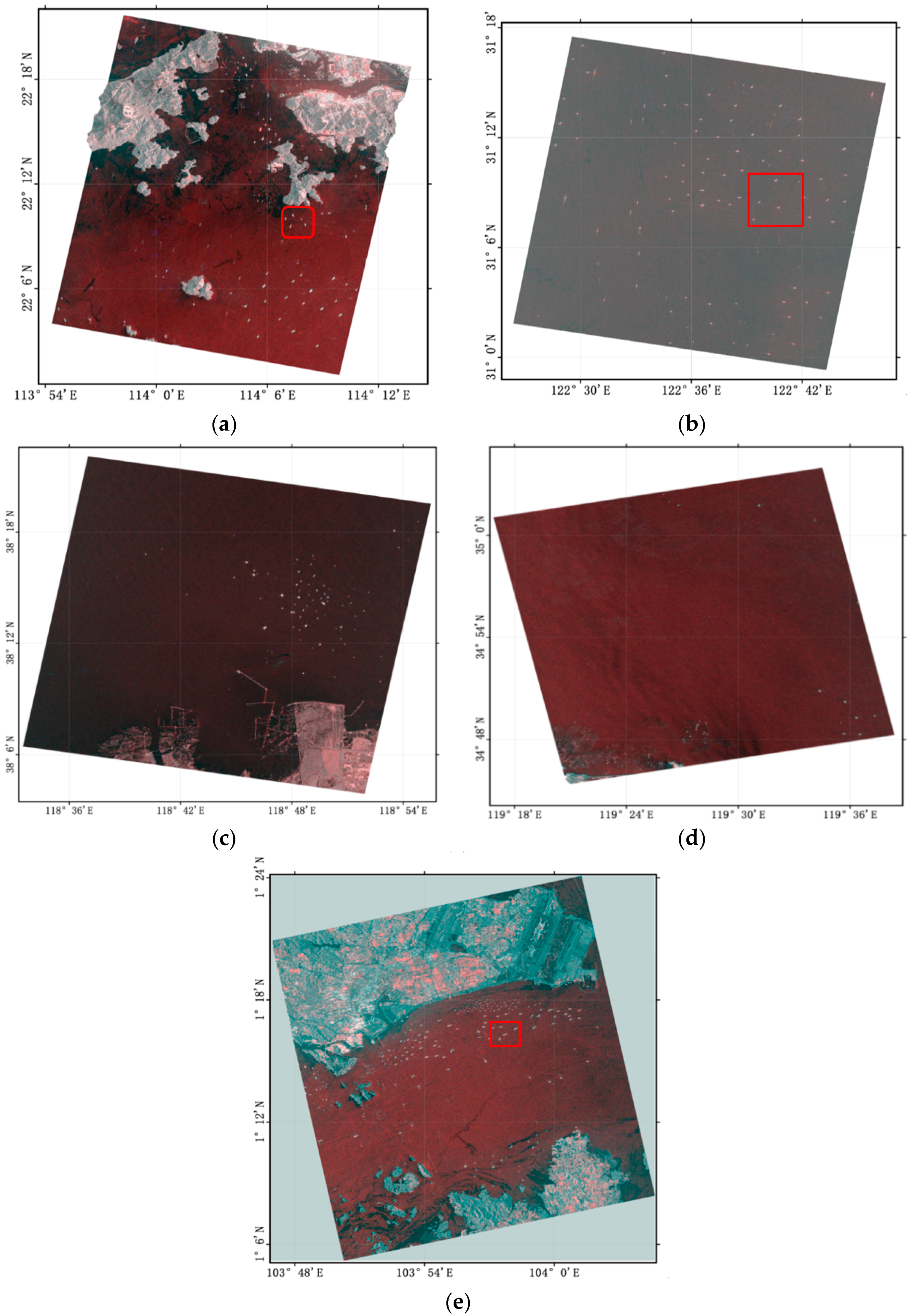
Figure 2a–e show the five RADARSAT-2 images with longitude and latitude information after geometric correction, among which, R = HH, G = HV and B = VH. The locations are the sea areas of the West Lamma Channel in Hong Kong, the Yangtze Estuary, the Yellow River Estuary, Lianyungang and Singapore, respectively. In these images, the bright dots with strong scattering echoes are ship targets, while the dark areas are the sea surface. The scattering echo intensity of the ship target is significantly greater than that of the sea surface. On the whole, many ships can be observed in Figure 2 except Figure 2d. In Figure 2a, the ships are located in the West Lamma Channel. In Figure 2c,e, the ships are mainly located near the port and shore, while in Figure 2b, there is no land area, the ships are mainly concentrated in the middle of the image, and some of the ships have strong crosswise side lobes.

The sea surface wind speeds are calculated by CMOD5 [24], which is a C-band geophysical model function for the inversion of the sea surface wind speed [25]. Combined with the Beaufort wind scale [26], the sea state in scene 04 reaches level 6, which belongs to the high sea state, and scene 03 belongs to the medium sea state; scenes 01–02 and 05 belong to the low sea state. The average wind speeds of the five images are listed in

Table 2. The average wind speed of five SAR images.

Scene ID	01	02	03	04	05
Average wind speed (m/s)	3.8	2.6	9.1	10.9	4.7
Sea state	3	2	5	6	3

.

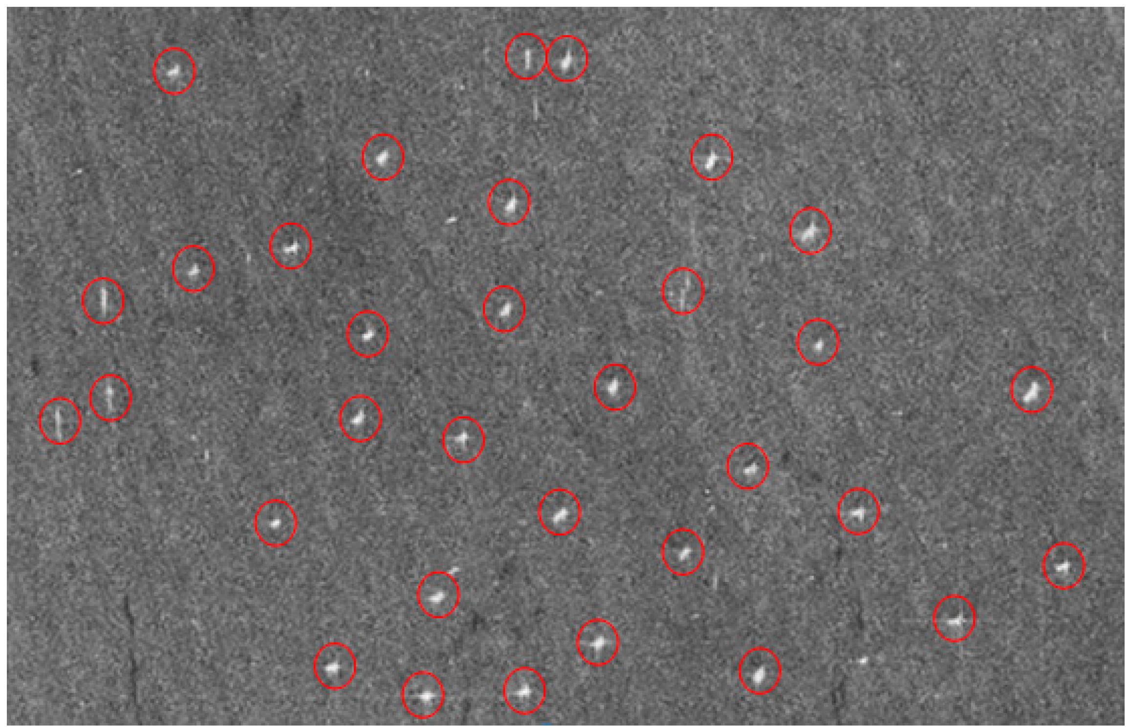
The ships in these five images are all matched by the Automatic Identification System (AIS) [27,28]. The AIS was developed primarily as a tool for maritime safety. The AIS equipment aboard vessels continuously and autonomously transmits information about the vessel including its identity, position, course and speed. Figure 3 is part of scene 02, and it shows the matching result, in which the SAR image contains 33 ships.

2.2. Extraction of Features from FP, CP and DP Data

2.2.1. Features from FP Data

First, we extracted several features by polarimetric decomposition, and the features are shown in

Table 3. Polarization features extracted under FP, CP and DP SAR modes.

FP SAR	CP SAR	DP SAR
Amplitudes: f1: |HH| f2: |HV| f3: |VV| f4: |HH-VV| f5: |HH+VV|	c1: |RH| c2: |RV|	d1: |HH| d2: |HV|
Polarimetric coherences: f6: HH/HV f7: HH/VV	c3: RH/RV	d3: HH/HV
Polarimetric phase differences:
f8: HH/HV f9: HH/VV	c4: RH/RV	d4: HH/HV
Eigenvalue parameters: f10: Entropy f11: Alpha f12: Anisotropy	c5: Entropy c6: Alpha	d5: Entropy d6: Alpha
Freeman decomposition: f13: Surface f14: Double f15: Volume Yamaguchi decomposition: f16: Surface f17: Double f18: Volume f19: Helix	Cloude decomposition: c7: Surface c8: Double c9: Random Raney decomposition: c10: DoP c11: Roundness c12: Delta c13: Surface c14: Double c15: Random

. The first column of Table 3 shows the features extracted from the FP data (f1–f16). The methods used in this paper are described below.

In FP mode, assuming that S_HV = S_VH, each pixel of an image can be represented by a linear scattering vector as follows:

$$k_L={[S_{HH}\sqrt{2}{S}_{HV}{S}_{VV}]}^T$$

(1)

where S_HH, S_HV, and S_VV are elements of the scattering matrix. The Pauli scattering vector enhances the scattering mechanism and is given by:

$$k_P=\frac{1}{\sqrt{2}}{[S_{HH}+S_{VV}{S}_{HH}-S_{VV}2S_{HV}]}^T$$

(2)

Features f1–f5 are defined as the amplitudes of the five polarization components introduced in Equations (1) and (2).

Features f6 and f7 are the polarimetric coherences of (HH, HV) and (HH, VV), respectively, and f8 and f9 are the phase differences of (HH, HV) and (HH, VV), respectively. The polarimetric coherence γ and phase difference $\Delta \varphi$ between HH and HV are described by

$${\gamma }_{HH/HV}=\frac{\left|\langle S_{HH}{S}_{HV}^{\ast }\rangle \right|}{\sqrt{\langle {\left|S_{HH}\right|}^2\rangle \langle {\left|S_{HV}\right|}^2\rangle }}$$

(3)

$$\Delta {\varphi }_{HH/HV}=\arg (\langle S_{HH}{S}_{HV}^{\ast }\rangle )$$

(4)

where $\langle \rangle$ indicates averaging in an 11 × 11 window. Features f10, f11, and f12 are the entropy, alpha, and anisotropy, respectively. These features are derived from eigenvalues analysis of the averaged coherency matrix T [29,30], $\langle T\rangle =\langle k_P{k}_P^{\ast T}\rangle$.

Features f13–f19 are components from a model-based decomposition. Among which, f13–f15 are amplitudes of surface scattering, double scattering and random scattering from Freeman decomposition, respectively [31]. Similarly, f16–f19 are amplitudes of surface scattering, double bounce, volume scattering, and helix scattering from Yamaguchi decomposition, respectively [32]. Based on the corresponding scattering mechanisms, the surface scattering, double scattering and random scattering from the Freeman decomposition are

$$\{\begin{array}{l}{P}_S={\mathrm{f}}_S(1+{\left|\beta \right|}^2)\\ P_D={\mathrm{f}}_D(1+{\left|\alpha \right|}^2)\\ P_V=f_V\end{array}$$

(5)

where $P_S+P_D+P_V={\left|S_{HH}\right|}^2+2{\left|S_{HV}\right|}^2+{\left|S_{VV}\right|}^2$ and α, β depend on the sign of $R\mathrm{e}(\langle S_{HH}{S}_{VV}^{\ast }\rangle )$. If $R\mathrm{e}(\langle S_{HH}{S}_{VV}^{\ast }\rangle )\ge 0$, surface scattering is dominant (α = −1); otherwise, double scattering is dominant (β = 1).

On the basis of three-component decomposition, Yamaguchi presented four-component decomposition [33]. In this decomposition method, $\langle S_{HH}{S}_{HV}^{\ast }\rangle \ne 0$ and $\langle S_{VH}{S}_{VV}^{\ast }\rangle \ne 0$ are introduced to show that the symmetry hypothesis is not true. The features f16, f17, f18, and f19 are defined as follows

$$\begin{array}{ll}{P}_S={\mathrm{f}}_S(1+{\left|\beta \right|}^2),& P_D={\mathrm{f}}_D(1+{\left|\alpha \right|}^2)\\ P_C=f_C,& P_V=f_V\end{array}$$

(6)

where $P_S+P_D+P_C+P_V={\left|S_{HH}\right|}^2+2{\left|S_{HV}\right|}^2+{\left|S_{VV}\right|}^2$ is the total scattering power.

2.2.2. Features from CP and DP Data

In this paper, to compare the performance among different polarization modes, the CP and DP data are simulated from the FP SAR data. We applied right-hand circular polarization (i.e., CTLR) [34,35] because circular transmission enables a better reconstruction of pseudo-FP information [36]. The CP data constructed from the FP data are shown as follows:

$${\left[\begin{array}{cc}{S}_{RH}& S_{RV}\end{array}\right]}^T={\left[\begin{array}{cc}{S}_{HH}-i{S}_{HV}& S_{VH}-i{S}_{VV}\end{array}\right]}^T$$

(7)

where S_RH and S_RV represent the scattering coefficients.

The second column of Table 3 (c1–c9) shows the features from the CP data. c1 and c2 are the amplitudes of S_RH and S_RV. c3 and c4 are the polarimetric coherence and phase difference between S_RH and S_RV, which we calculated using the same formulas as (3) and (4). Features c5 and c6 are the entropy and the alpha angle, respectively, extracted from the reconstructed coherency matrix proposed by Nord [36]. The formulas are

$$\{\begin{array}{l}{H}_{CTLR}=-{\displaystyle \sum _{i=1}^2{p}_{i}lo{g}_2{p}_i}\\ \alpha ={\displaystyle \sum _{i=1}^2{p}_i{\alpha }_i}\end{array}$$

(8)

respectively, where $p_i={\lambda }_i/{\displaystyle {\sum }_{i=1}^2{\lambda }_i}$, ${\alpha }_i$ is an eigenvector corresponding to ${\lambda }_i$, and i = 1,2…. c7–c9 are the components of a Cloude decomposition [37]. The formulas are

$$P_S=\frac{1}{2}{g}_{0}m(1+\cos 2{\alpha }_s)$$

(9)

$$P_d=\frac{1}{2}{g}_{0}m(1-\cos 2{\alpha }_s)$$

(10)

$$P_v=g_0(1-m)$$

(11)

respectively, where ${\alpha }_s=1/2{\tan }^{-1}(\sqrt{g_1^2+g_2^2}/(-g_3))$. c10–c15 are components from Raney’s decomposition using the Stokes parameters of the scattering matrix [34,38]. The formulas are

$$m=\frac{{(g_1^2+g_2^2+g_3^2)}^{1/2}}{g_0}0<m<1\tan \delta =-\frac{g_3}{g_2}\sin 2\chi =-\frac{g_3}{m{g}_0}$$

(12)

$${\left[\begin{array}{c}{P}_d\\ P_v\\ P_s\end{array}\right]}_{m-\delta }=\left[\begin{array}{c}{(m{g}_0\frac{1-\sin \delta }{2})}^{1/2}\\ {(g_0(1-m))}^{1/2}\\ {(m{g}_0\frac{1+\sin \delta }{2})}^{1/2}\end{array}\right]$$

(13)

The third column of Table 3 shows the features from the DP data, the first four of which are extracted from FP features: d1 = f1, d2 = f2, d3 = f6, and d4 = f8. d5 and d6 are the pseudo entropy and the alpha angle, respectively, and are calculated from the eigenvalue analysis of a 2 × 2 covariance matrix [39,40].

2.3. Sample Selection

To assess the performance of features for ship detection, we select samples with ships only, samples with sea only and samples with both ships and sea. The numbers of regions of interest in the samples are 75, 75 and 50, respectively.

3. Comprehensive Quantification and Evaluation of Features for Ship Detection

First, we introduce the Euclidean distance to quantitatively evaluate the capacity of features for detecting ships. Then, we identify good features for ship detection by measuring the redundancy via the mutual information. The results can provide a reference for feature selection in practical applications.

3.1. Evaluation of Different Features by Euclidean Distance

Based on the features’ scattering differences, the Euclidean distance between ships and the surrounding sea area is used to evaluate the performance of 40 features extracted from FP, CP and DP decomposition. The distance is defined as in [41]:

$$D=\frac{\left|M_{SHIP}-M_{SEA}\right|}{\sqrt{{\sigma }_{SHIP}^2+{\sigma }_{SEA}^2}}$$

(14)

where $M_{SHIP}$ and $M_{SEA}$ correspond to the statistical average of the samples of ships and the sea surface, respectively, and ${\sigma }_{SHIP}^2$ and ${\sigma }_{SEA}^2$ denote the variance in ships and sea surface, respectively. This equation implies that the larger the distance is, the better the performance of the features in distinguishing ships from the surrounding sea.

The five RADARSAT-2 images in Table 1 are used to calculate the Euclidean distance. For each image, we use 30 regions of interest: 15 ship samples and 15 surrounding sea samples. The final Euclidean distance is the average of the 15 calculated values.

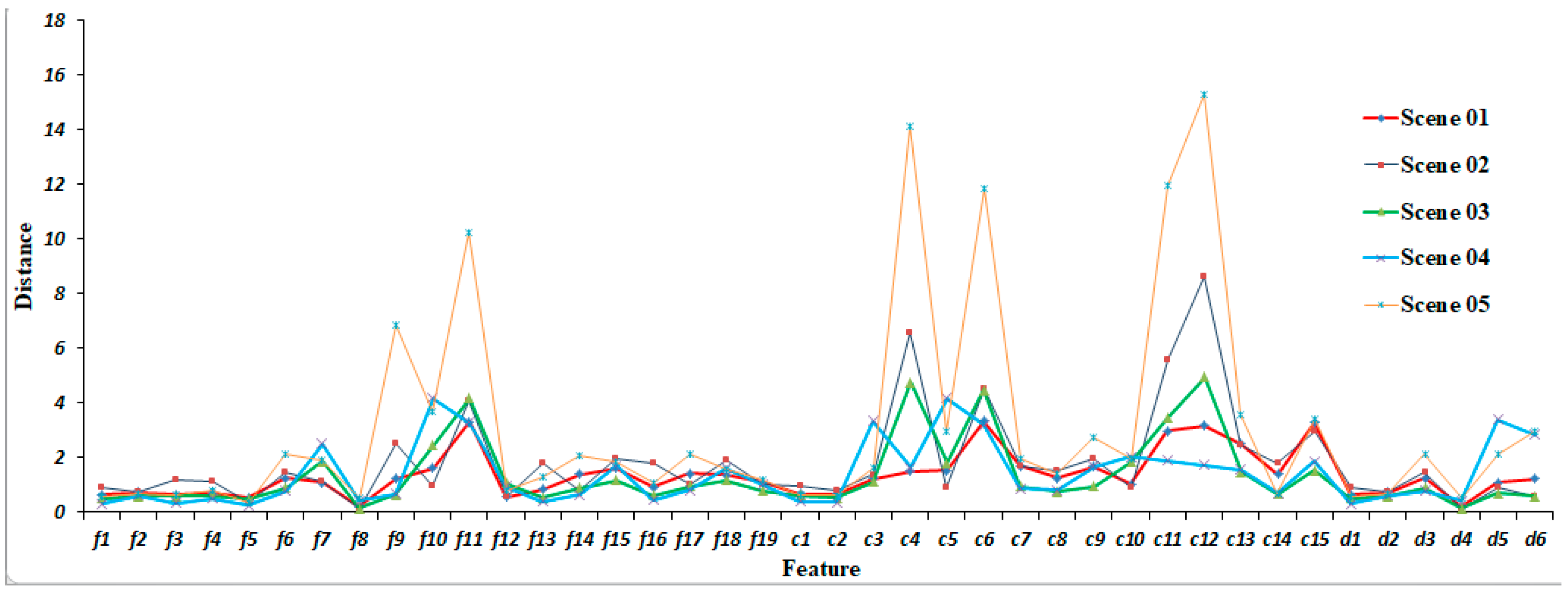
Figure 4 shows the distances between ships and the sea area for f1–f19, c1–c15, and d1–d6. In general, the trend in the distance between different features is consistent in the five images. The distances between features in CP mode are generally larger than those in FP and DP mode; the next largest distances between features are in FP mode, and the distances between features in DP mode are the smallest, especially in scenes 02 and 05. Therefore, the features from CP mode are more suitable for ship detection than those from FP and DP mode. Moreover, with larger distances, f9, f11, c4, c6, c11 and c12 have good ship detection performance. In each scene, the values of these six features are several to more than ten times the values of the other polarization features, especially in scene 05. Then, f7, c5, c15 and d5 are smaller than f9, f11, c4, c6, c11 and c12 but larger than the other features. Note that the distances of c4, c6, c11 and c12 are larger than 10 in scene 05, which indicates the best ship detection performance among these features out of scenes 01–05.

3.2. Mutual Information Analysis

Based on the selected features in Section 3.1, the information from the features (f7, f9, f11, c4, c5, c6, c11, c12, c15 and d5) should be quantified for better accuracy and efficiency in ship detection. The relevance between ships and features, and the redundancy among different features, should be further evaluated. Mutual information is a correlation measure based on the information-theoretical concept of entropy and has become an important measure in the analysis of informational content [42,43,44].

Given two random variables X and Y, the mutual information is defined as

$$I(X|Y)=H(X)-H(X|Y)$$

(15)

where H(X) denotes the entropy of X and H(X|Y) denotes the conditional entropy of X given Y. The formulas of H(X) and H(X|Y) are

$$H(X)=-{\displaystyle \sum _{i}P(x_i){\log }_2(P(x_i))}$$

(16)

$$H(X|Y)=-{\displaystyle \sum _{j}P(y_j)}{\displaystyle \sum _{i}P(x_i|y_j){\log }_2(P(x_i|y_j))}$$

(17)

where P(x_i) are the prior probabilities for all values of X and P(x_i|y_j) are the posterior probabilities of X given the values of Y.

The intuitive concept behind this definition of I describes the fraction of information that is shared mutually by both X and Y, called “information overlap.” Moreover, the mutual information I(X|Y) is symmetric in X and Y, which means that I(X|Y) = I(Y|X) in a strictly mathematical sense. We normalize I(X|Y) by dividing it by H(X) + H(Y) to achieve increased comparability. The formula is as follows:

$$SU(X,Y)=\frac{I(X|Y)}{H(X)+H(Y)}$$

(18)

Twenty regions of interest are selected to calculate the normalized mutual information. The final mutual information value is the average of the calculated values.

Table 4. Normalized mutual information of ship and feature.

Feature	f7	f9	f11	c4	c5	c6	c11	c12	c15	d5
I(x|y)	0.383	0.522	0.603	0.610	0.519	0.625	0.658	0.631	0.315	0.359

shows the normalized mutual information of the ships and features. In this case, X is a ship and Y is a feature, and a high mutual information I implies a strong predictive value of feature Y for identifying ship X. The values of f11, c4, c6, c11 and c12 are greater than 0.6, which indicates a high relevance between the ship and the feature, and this is consistent with the conclusion mentioned in section A. The performance of the features selected above is thus further confirmed.

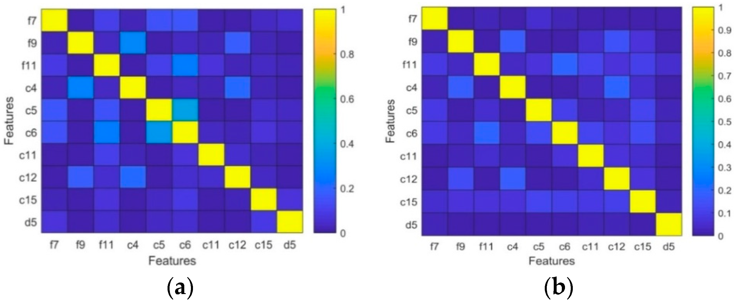
Figure 5 shows the normalized mutual information of features. Figure 5a,b are symmetric about the main diagonal, which confirms the symmetry of the mutual information mentioned above. Furthermore, the normalized mutual information between a feature and itself is 1, while the values among different features are less than 1. In general, the trends in the normalized mutual information values in (a) and (b) are consistent with low information redundancy. The features in CP and FP mode have a higher relevance than the features in DP mode, which may be due to the loss of polarization information in DP mode. In detail, the feature pairs with relatively high information overlap are (f11, c6), (f9, c4) and (c5, c6). Among these, f11 and c6 represent the alphas extracted from the H/alpha decompositions; f9 and c4 represent the polarimetric coherence extracted from HH/VV and RH/RV, respectively; and c5 and c6 represent the entropy and alpha extracted from the H/alpha decomposition, respectively. This result indicates that features from the same polarimetric decomposition have higher redundancy. For the feature pairs, (f7, c5), (f7, c6), (f9, c12), (c4, c12) and (c6, c11) have a lower redundancy than (f11, c6), (f9, c4) and (c5, c6). There is little information overlap between both c15 and d5 and the other features. Hence, combined with the Euclidean distance and normalized mutual information, c4, c6, c11 and c12 are selected for further study.

4. A New Feature: Phase Factor

Section 3 concludes that the features in CP mode are more suitable than the DP and FP modes for ship target detection. Therefore, in this section, the features in CP mode are further studied. To analyze the theoretical ship detection performance of features, the relationship between the coherency matrix and the Stokes vector is established. Then, the X-Bragg scattering model is introduced to describe the Stokes vector. Finally, a new feature, which has a good ship detection performance, is proposed.

In CTLR mode, the radar antenna transmits a circular signal and simultaneously receives two orthogonal linear polarization signals. Consider a radar that transmits a right circular signal. The scattering vector [37,45] is

$${\overrightarrow{k}}_l={[E_{RH}{E}_{RV}]}^T=\frac{1}{\sqrt{2}}{(S_{HH}-j{S}_{HV},-j{S}_{VV}+S_{HV})}^T$$

(19)

The coherency matrix T is defined by Huynen parameters [46]:

$$T={\overrightarrow{k}}_p{\overrightarrow{k}}_p^H=\left[\begin{array}{ccc}{T}_{11}& T_{12}& T_{13}\\ T_{21}& T_{22}& T_{23}\\ T_{31}& T_{32}& T_{33}\end{array}\right]=\left[\begin{array}{ccc}2A_0& C-jD& H+jG\\ C+jD& B_0+B& E+jF\\ H-jG& E-jF& B_0-B\end{array}\right]$$

(20)

where ${\overrightarrow{k}}_p=1/\sqrt{2}{\left[S_{HH}+S_{VV}{S}_{HH}-S_{VV}2S_{HV}\right]}^T$, and A₀, B, B₀, C, D, E, F, G, and H are the Huynen parameters. Note that A₀, B₀, and F are rotation invariants.

Matrix T can be expressed by S_HH, S_HV, and S_VV, but it is extremely complicated [32]. In this case, a new idea is proposed by using the elements of the scattering vector:

$$\{\begin{array}{l}{E}_{RH}+\mathrm{j}{E}_{RV}=S_{HH}+S_{VV}\\ E_{RH}-\mathrm{j}{E}_{RV}=S_{HH}-S_{VV}-2j{S}_{HV}\end{array}$$

(21)

Then, a new matrix Y is given by

$$\begin{array}{cc}\hfill Y& =\left[\begin{array}{l}{E}_{RH}+\mathrm{j}{E}_{RV}\\ E_{RH}-\mathrm{j}{E}_{RV}\end{array}\right]\left[\begin{array}{cc}{(E_{RH}+\mathrm{j}{E}_{RV})}^H& {(E_{RH}-\mathrm{j}{E}_{RV})}^H\end{array}\right]\hfill \\ & =\left[\begin{array}{l}{S}_{HH}+S_{VV}\\ S_{HH}-S_{VV}-2j{S}_{HV}\end{array}\right]\left[\begin{array}{cc}{(S_{HH}+S_{VV})}^H& {(S_{HH}-S_{VV}-2j{S}_{HV})}^H\end{array}\right]\hfill \\ & =\left[\begin{array}{cc}(S_{HH}+S_{VV}){(S_{HH}+S_{VV})}^{\ast }& (S_{HH}+S_{VV})({(S_{HH}-S_{VV})}^{\ast }+2\mathrm{j}{S}_{HV}^{\ast })\\ (S_{HH}-S_{VV}-2j{S}_{HV}){(S_{HH}+S_{VV})}^{\ast }& (S_{HH}-S_{VV}-2j{S}_{HV})({(S_{HH}-S_{VV})}^{\ast }+2\mathrm{j}{S}_{HV}^{\ast })\end{array}\right]\hfill \end{array}$$

(22)

Combined with matrix T and the Huynen parameters, matrix Y can be obtained:

$$Y=\left[\begin{array}{cc}{T}_{11}& T_{12}+j{T}_{13}\\ T_{12}^{\ast }-j{T}_{13}^{\ast }& T_{22}+T_{33}-2\mathrm{Im}(T_{23})\end{array}\right]=\left[\begin{array}{cc}2A_0& (C-G)+j(H-D)\\ (C-G)-j(H-D)& 2(B_0-F)\end{array}\right]$$

(23)

In [46], the Stokes vector of the scattered wave in CTLR mode is written as

$$g=\left[\begin{array}{c}{g}_0\\ g_1\\ g_2\\ g_3\end{array}\right]=\left[\begin{array}{c}{A}_0+B_0-F\\ C-G\\ H-D\\ -A_0+B_0-F\end{array}\right]$$

(24)

Therefore, Y can be derived from Equations (23) and (24):

$$Y=\left[\begin{array}{cc}{T}_{11}& T_{12}+\mathrm{j}{T}_{13}\\ T_{12}^{\ast }-j{T}_{13}^{\ast }& T_{22}+T_{33}-2\mathrm{Im}(T_{23})\end{array}\right]=\left[\begin{array}{cc}{\mathrm{g}}_0-g_3& {\mathrm{g}}_1+j{g}_2\\ {\mathrm{g}}_1-j{g}_2& {\mathrm{g}}_0+g_3\end{array}\right]$$

(25)

As a result, the Stokes vector is described by the coherency matrix:

$$\{\begin{array}{l}{\mathrm{g}}_0=\frac{T_{11}+T_{22}+T_{33}}{2}-\mathrm{Im}(T_{23})\\ {\mathrm{g}}_1=\mathrm{Re}(T_{12})-\mathrm{Im}(T_{13})\\ g_2=\mathrm{Im}(T_{12})+\mathrm{Re}(T_{13})\\ g_3=\frac{-T_{11}+T_{22}+T_{33}}{2}-\mathrm{Im}(T_{23})\end{array}$$

(26)

Based on the theory mentioned above, the coherency matrix T is used to represent the Stokes vector through the constructed matrix Y. For a better description of the features, the X-Bragg scattering model is introduced below.

The X-Bragg scattering model was first introduced by Hajnsek to solve the case of nonzero cross-polarized backscattering and depolarization [23]. By assuming a roughness disturbance-induced random surface slope β, X-Bragg scattering is modeled as a reflection depolarizer by rotating the Bragg coherency matrix about an angle β and performing configurational averaging over a given distribution P(β):

$$[T]={\displaystyle {\int }_0^{2\pi }[T(\beta )]}P(\beta )d\beta$$

(27)

assuming that P(β) is a uniform distribution of approximately zero with width β₁ (β₁ < π/2). The width β₁ describes the roughness component of the sea surface. The coherency matrix for the rough surface becomes Equation (28) with $\sin c(x)=\sin (x)/x$.

$$T_{X\text{-}B\mathrm{ragg}}=\left[\begin{array}{ccc}{T}_{11}& T_{12}& T_{13}\\ T_{21}& T_{22}& T_{23}\\ T_{31}& T_{32}& T_{33}\end{array}\right]=\left[\begin{array}{ccc}{C}_1& C_2\sin c(2{\beta }_1)& 0\\ C_2\sin c(2{\beta }_1)& C_3(1+\sin c(4{\beta }_1))& 0\\ 0& 0& C_3(1-\sin c(4{\beta }_1))\end{array}\right]$$

(28)

where

$$\{\begin{array}{c}{C}_1={\left|R_S+R_P\right|}^2={\left|S_{HH}+S_{VV}\right|}^2/2\\ C_2=(R_S+R_P)(R_S^{\ast }-R_P^{\ast })=(S_{HH}+S_{VV}){(S_{HH}-S_{VV})}^{\ast }/2\\ C_3=\frac{1}{2}{\left|R_S-R_P\right|}^2={\left|S_{HH}-S_{VV}\right|}^2/4\end{array}$$

Substituting Equation (28) into Equation (26), the Stokes vector in CP SAR can be described by an X-Bragg scattering matrix

$$\{\begin{array}{l}{\mathrm{g}}_0=\frac{T_{11}+T_{22}+T_{33}}{2}-\mathrm{Im}(T_{23})=\frac{C_1+2C_3}{2}\\ {\mathrm{g}}_1=\mathrm{Re}(T_{12})-\mathrm{Im}(T_{13})=\mathrm{Re}(C_2\sin c(2{\beta }_1))\\ g_2=\mathrm{Im}(T_{12})+\mathrm{Re}(T_{13})=\mathrm{Im}(C_2\sin c(2{\beta }_1))\\ g_3=\frac{-T_{11}+T_{22}+T_{33}}{2}-\mathrm{Im}(T_{23})=\frac{-C_1+2C_3}{2}\end{array}$$

(29)

Note that $g_0$ and $g_3$ are rotation invariants because they are independent of ${\beta }_1$, while $g_1$ and $g_2$ are related to the rotation angle ${\beta }_1$. Hence, the features described by $g_0$ and $g_3$ are stable for separating ships from sea, even in a high sea state.

For a better explanation of the features with strong ship detection abilities, the roundness (c11), delta (c12) and the HESA [16] are listed as examples. Combined with the model derived from Equation (29), the polarization features are derived by the X-Bragg scattering matrix, which shows the scattering difference between ships and the sea surface. On this basis, a new feature, the phase factor, is presented.

4.1. Roundness

The formula of roundness is

$$\sin 2\chi =-\frac{g_3}{\sqrt{g_1^2+g_2^2+g_3^2}}$$

(30)

According to Equations (29) and (30), roundness is given by

$$\sin 2\chi =\frac{C_1-2C_3}{\sqrt{4{(C_2\sin c(2{\beta }_1))}^2+(-C_1+2C_3{)}^2}}$$

(31)

In Equation (31), the sign of the roundness is consistent with that of $\sin 2\chi$. On the right side of Equation (31), the denominator is positive, so the sign of the roundness depends on the sign of the numerator. The numerator of Equation (31) can be derived as

$$C_1-2C_3=2\mathrm{Re}(S_{HH}{S}_{VV}^{\ast }))$$

(32)

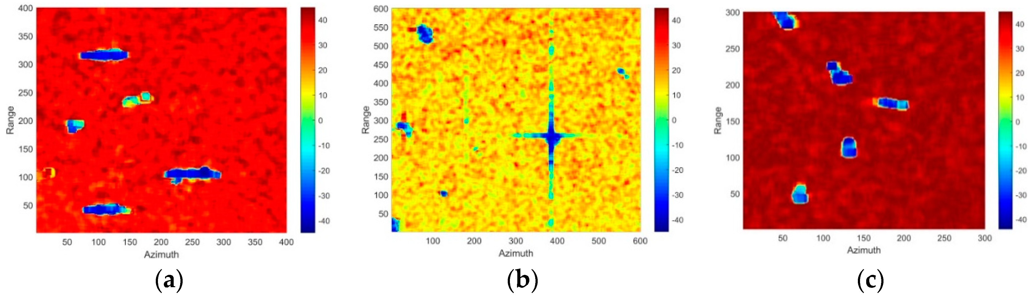
As shown in Equation (32), the value of C₁–2C₃ is depends on $\mathrm{Re}(S_{HH}{S}_{VV}^{\ast })$. When single scattering is dominant, the sign of $\mathrm{Re}(S_{HH}{S}_{VV}^{\ast })$ is positive, and when even scattering is dominant, the sign of $\mathrm{Re}(S_{HH}{S}_{VV}^{\ast })$ is negative [47]. In fact, the sea surface is mainly characterized by single scattering, while ships are mainly characterized by even scattering. Consequently, the value of the sea surface should be positive, and the value of a ship should be negative. The areas shown in Figure 6a–c represent the red box insets shown in Figure 2a,b,e. The images are derived from RADARSAT-2 scenes 01, 02 and 05 respectively, which were each acquired at low sea state. The ships and the sea surface can be separated by a constant 0 in the feature roundness. Note that there exists a “ship” in the lower left corner of (a) without AIS information, so it is uncertain whether it is a ship or not.

Combined with Equations (29) and (31), the roundness is related to angle ${\beta }_1$, which means that a higher sea state can lead to a decline of the roundness detector’s performance. What’s worse, small ships even cannot be distinguished from the sea clutter.

4.2. Delta

The formula for delta is

$$\delta ={\tan }^{-1}(\frac{g_3}{g_2})$$

(33)

Then, delta is obtained by substituting Equation (29) into Equation (33):

$$\delta =-\frac{1}{\sin c(2{\beta }_1)}\frac{\mathrm{Re}(S_{HH}{S}_{VV}^{\ast })}{\mathrm{Im}(S_{HH}{S}_{VV}^{\ast })}$$

(34)

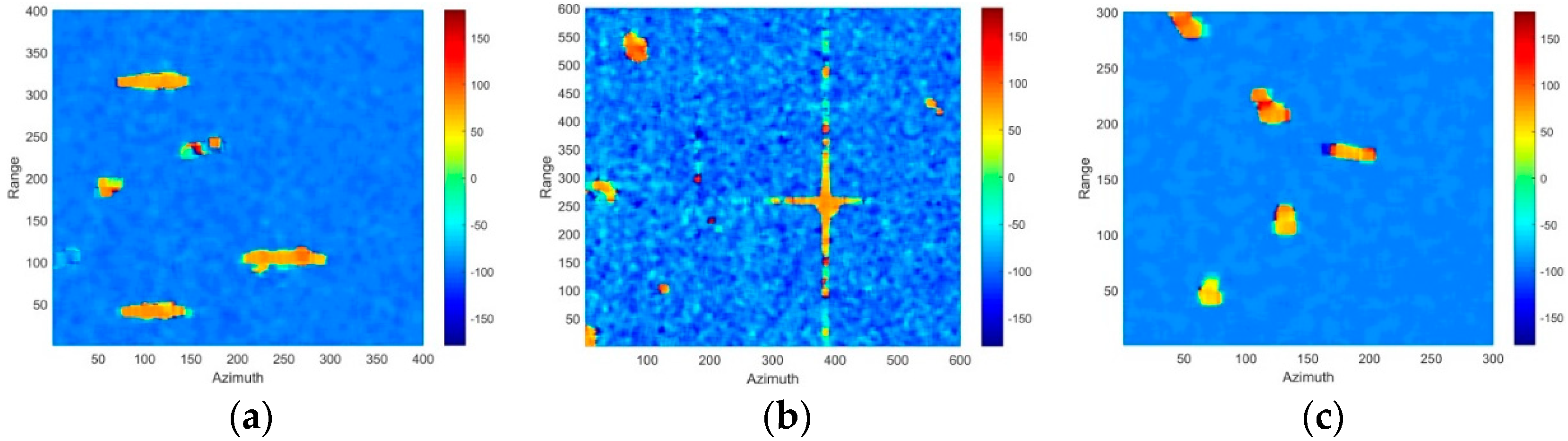
In Equation (34), for single scattering, the sign of delta is negative; for even scattering, the sign of delta is positive [47]. Due to the scattering differences, ships in the SAR image are mainly characterized by even scattering, while the sea is mainly characterized by single scattering. Therefore, the sign of delta for ships should be positive, and the sign of delta for the sea surface should be negative. The areas shown in Figure 7a–c represent the red box insets shown in Figure 2a,b,e. The images are derived from RADARSAT-2 scenes 01, 02 and 05 respectively, which were each acquired at low sea state. The constant 0 can be used to distinguish ships from the sea surface in the feature delta.

Note that the value of delta is related to angle ${\beta }_1$ in Equation (34), and the surface roughness increases with the increasing sea state. Therefore, the value of delta is unstably influenced by ${\beta }_1$, making it difficult to use in distinguishing ships and the sea surface in a high sea state.

4.3. HESA

The formula of the HESA is

$$HESA=\sqrt{g_0{H}_{\omega }}$$

(35)

where

$$H_{\omega }=-{\displaystyle \sum _{i=1}^2{p}_i{\log }_2{p}_i},p_{1,2}=\frac{g_0\pm \sqrt{g_1^2+g_2^2+g_3^2}}{2g_0}$$

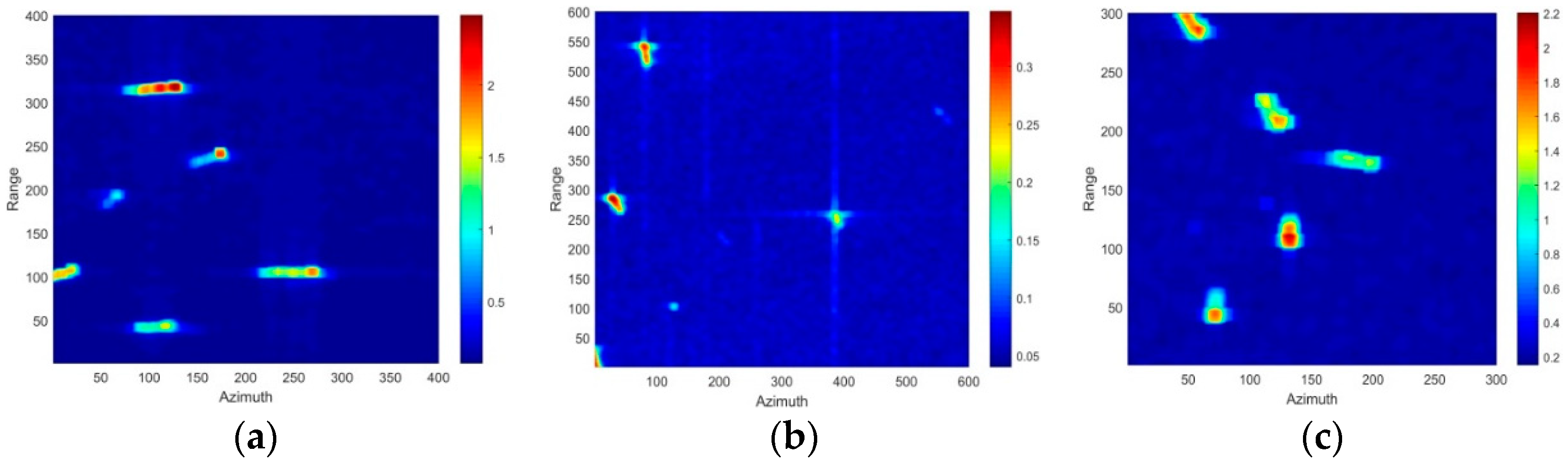
The areas shown in Figure 8a–c represent the red box insets shown in Figure 2a,b,e. The images are derived from RADARSAT-2 scenes 01, 02 and 05 respectively, which were each acquired at low sea state. In Equation (35), the value of the HESA is positive, as shown in Figure 8, and the outlines of ships are clear. However, the HESA is related not only to the dielectric constant and the incidence angle but also to the rotation angle ${\beta }_1$. ${\beta }_1$ represents the sea surface roughness, and the HESA may cause a severe decline when the sea state is high. The constant 1 can be selected to separate ships from the sea surface.

4.4. Phase Factor

Based on the analysis of the above features, a new feature $\varsigma$, called the phase factor, is presented in this paper. The formula of the phase factor is

$$\varsigma ={\tan }^{-1}(\frac{g_0}{g_3})$$

(36)

Combined with Equation (29), the phase factor can be derived by

$$\varsigma ={\tan }^{-1}(\frac{g_0}{g_3})={\tan }^{-1}(\frac{T_{11}+T_{22}+T_{33}-2\mathrm{Im}(T_{23})}{-T_{11}+T_{22}+T_{33}-2\mathrm{Im}(T_{23})})={\tan }^{-1}(\frac{C_1+2C_3}{-C_1+2C_3})$$

(37)

Equivalently,

$$\begin{array}{cc}\hfill \tan \varsigma & =\frac{C_1+2C_3}{-C_1+2C_3}=\frac{{\left|R_S-R_P\right|}^2+{\left|R_S+R_P\right|}^2}{{\left|R_S-R_P\right|}^2-{\left|R_S+R_P\right|}^2}\hfill \\ & =\frac{{\left|S_{HH}-S_{VV}\right|}^2+{\left|S_{HH}+S_{VV}\right|}^2}{{\left|S_{HH}-S_{VV}\right|}^2-{\left|S_{HH}+S_{VV}\right|}^2}=\frac{{\left|S_{HH}-S_{VV}\right|}^2+{\left|S_{HH}+S_{VV}\right|}^2}{-4\mathrm{Re}(S_{HH}{S}_{VV}^{\ast })}\hfill \end{array}$$

(38)

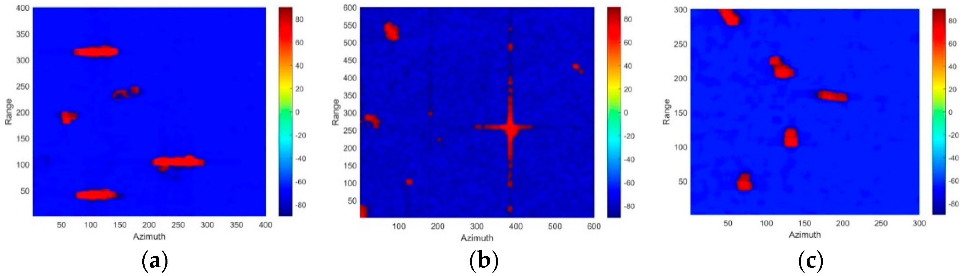
In Equation (38), the sign of the phase factor depends on the sign of $-\mathrm{Re}(S_{HH}{S}_{VV}^{\ast })$. For single scattering, the value of $\mathrm{Re}(S_{HH}{S}_{VV}^{\ast })$ is positive, so the value of the phase factor is negative; for even scattering, the value of the phase factor is positive [47]. Considering that ships are mainly characterized by even scattering, while sea surfaces are mainly characterized by single scattering, the sign of ships is positive, and the sign of the sea surface is negative. In other words, the phase factor is able to distinguish single scattering and even scattering to determine the dominant scattering mechanism. When the phase factor is positive, the even scattering is stronger than the surface scattering; when the phase factor is negative, the surface scattering is stronger than the even scattering. The areas shown in Figure 9a–c represent the red box insets shown in Figure 2a,b,e. The images are derived from RADARSAT-2 scenes 01, 02 and 05 respectively, which were each acquired at low sea state. In Figure 9, the sign of ships is positive, while the sign of the sea surface is negative, which means that the constant 0 can be used to distinguish ships and sea surface.

Furthermore, Equation (38) shows that the value of the phase factor is related only to the dielectric constant and incident angle and is independent of the random surface slope ${\beta }_1$. This finding indicates that the phase factor is rotation invariant and stable to different sea states (especially the high sea state), which is of great benefit to ship detection. Therefore, the phase factor theoretically achieves a better detection performance than the other abovementioned polarization features.

5. Detection Results and Discussion

In this section, experiments were performed using CTLR mode emulated from C-band RADARSAT-2 FP SAR data to validate the superiority of the phase factor in ship detection. The phase factor is compared with the roundness, delta, HESA and CFAR detectors, respectively.

5.1. Comparisons Between Phase Factor and Roundness, Delta, HESA Detectors

In this section, comparisons are made among roundness, delta, HESA and phase factor detectors by analyzing the scattering difference between ships and the sea surface.

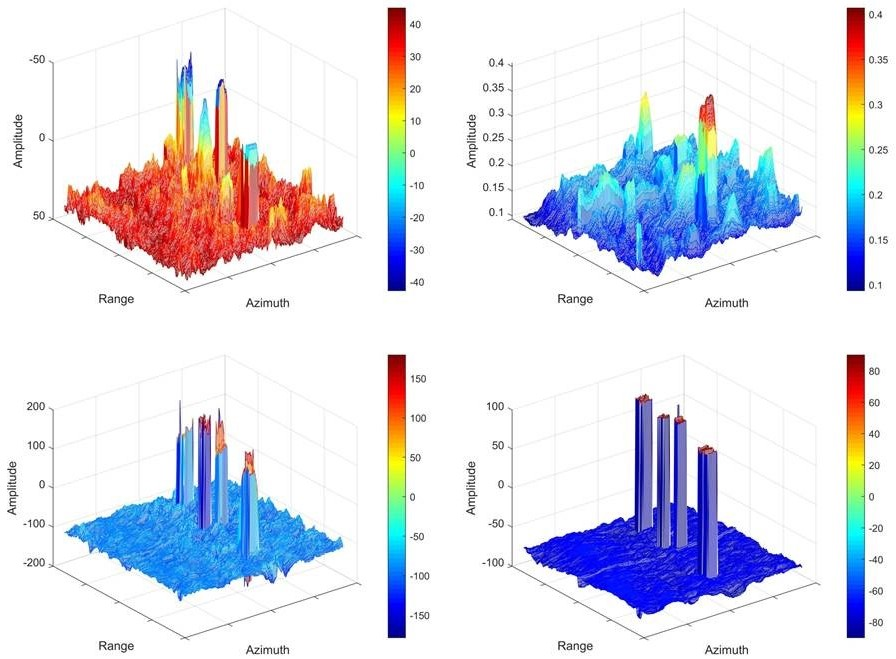
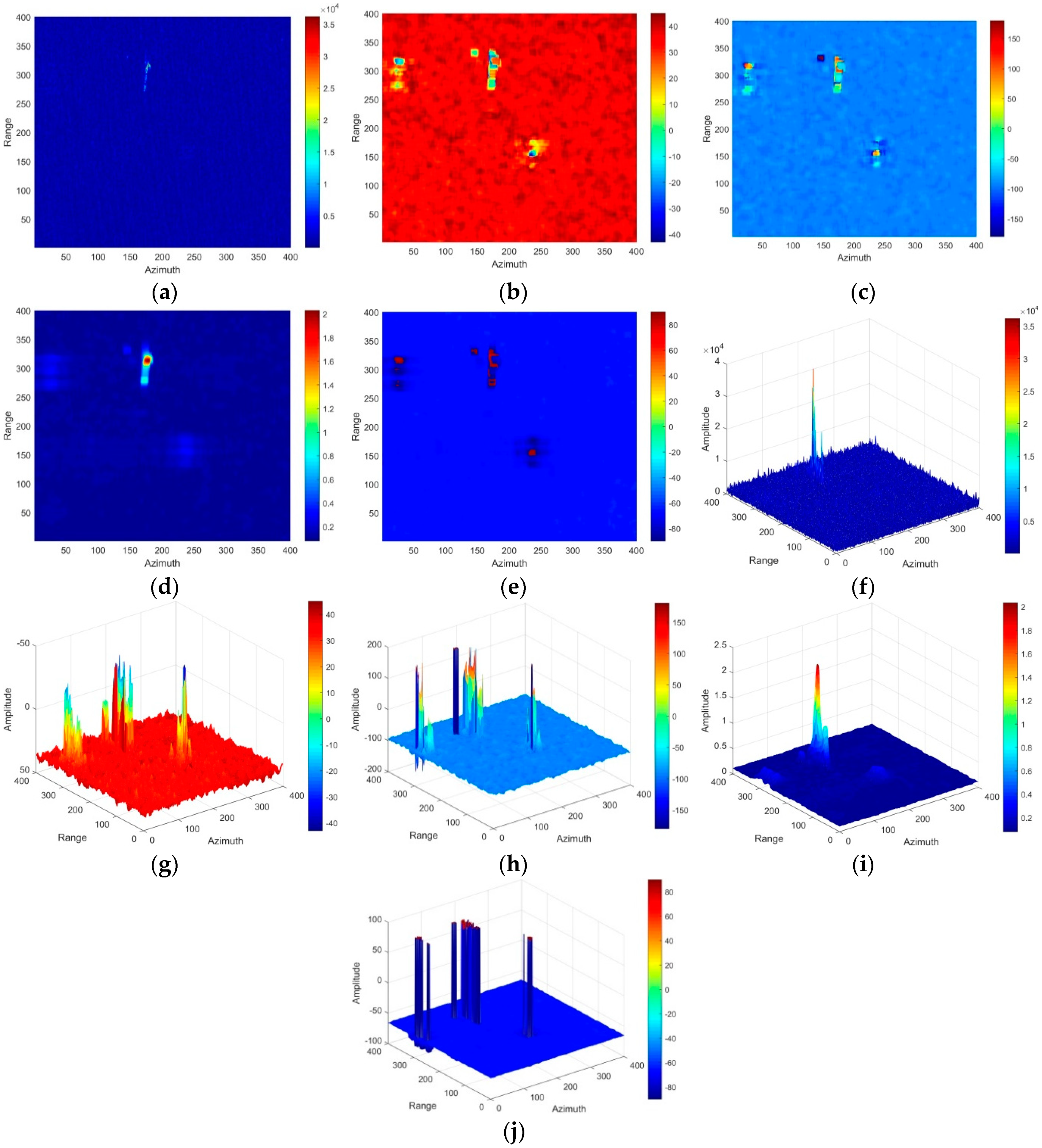
Two experiments comparing five detectors in ship detection are performed, as shown in Figure 10 (#1) and Figure 11 (#2). Figure 10 shows the detection results in a medium sea state. The roundness, delta, the HESA and the phase factor perform better than the amplitude in detection tasks because the detected ships in (b)–(f) all have clear outlines, and the ship pixels were very bright with respect to the surrounding sea clutter. The results indicate that the four features from CP decomposition can effectively distinguish ships from sea clutter. In (a), (d), (f) and (i), only one ship is detected by the amplitude and HESA, while three ships are detected by the other three features. For the roundness, delta and phase factor, the signs of the ship and sea clutter data are opposites, which facilitate distinguishing ships from the sea clutter by means of a constant 0. For the HESA, the signs of ships and sea clutter data are all positive, so it is hard to select a proper value to separate ships from sea surface. Note that the spans of the roundness, delta and the phase factor are dozens of times larger than that of the HESA.

For the sake of fairness, $P=\left|M_{SHIP}-M_{SEA}\right|/\max f$ is used to evaluate the ship detection performance, where $M_{SHIP}$ and $M_{SEA}$ correspond to the statistical average of the samples of ships and sea surface, respectively, and f represents features. Note that P ranges from 0 to 2, which can describe the scattering difference and can distinguish ships from the surrounding sea surface. This finding indicates that the higher the value P, the better the detection performance is. The results are listed in

Table 5. Performances comparison of the five detectors.

Feature	Experiment no.	Amplitude	Roundness	Delta	HESA	Phase Factor
P	#1	0.02	1.07	0.82	0.18	1.29
	#2	0.05	1.37	1.19	0.32	1.83
Multiples	#1	1	54	41	9	65
	#2	1	27	24	7	37

. Multiples represent the performance ratio of the roundness, delta, HESA or phase factor to the amplitude.

The performances of five detectors are listed in descending order: phase factor, roundness, delta, HESA, and amplitude of RV polarization. Note that the performances of the phase factor, roundness, delta, and the HESA are 65, 54, 41 and 9 times the amplitude of RV polarization, respectively. Thus, according to the value and the scattering difference between the ships and the sea surface, the phase factor can detect ships better than the other four detectors. In another respect, the phase factor is irrelevant to the sea surface roughness, and thus it is sufficiently stable with an increasing sea state, as shown in (e) and (j). In contrast, the roundness, delta and HESA are related to the sea surface roughness. The sea surface is very rough in a high sea state, and sea spikes can cause false alarms and an increased difficulty in the detection.

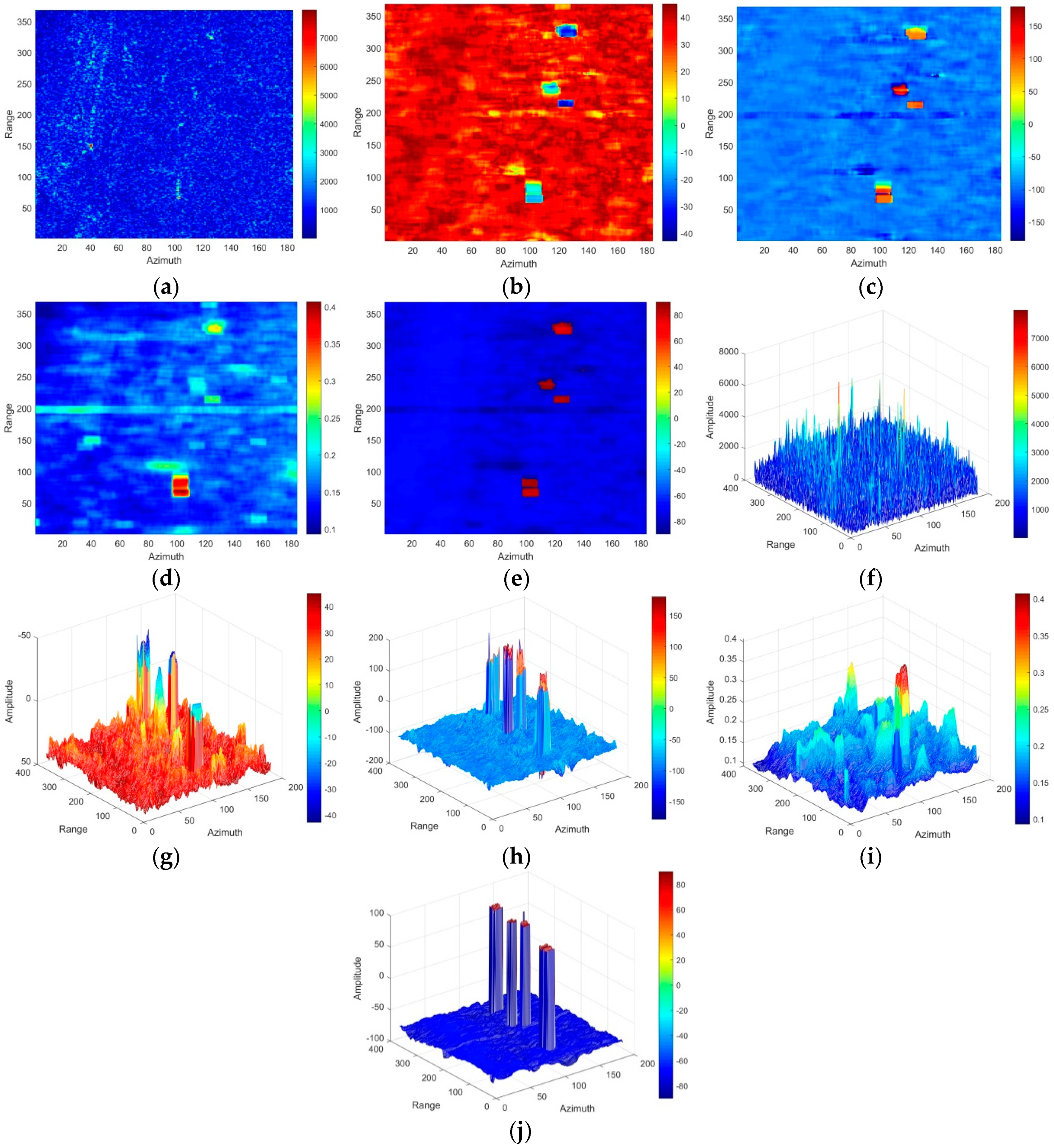
Figure 11 is another comparison of the detectors in a high sea state (#2). Combined with the AIS, the image contains four small ships. All the ships can be detected with the five detectors. Influenced by strong winds, many false alarms appear in (b)–(d) and (g)–(i), resulting in the severe performance degradation of the roundness and HESA detectors.

The performances of the five detectors are shown in Table 5, which are consistent with results from #1. The performances of the phase factor, roundness, delta, and HESA are 37, 27, 24 and 7 times that of the amplitude of the RV polarization, respectively. According to the performance ratio, although the detectors in a high sea state are smaller than those in a medium state, the phase factor is always the best among the five detectors. The results demonstrate that the phase factor is an effective detector with strong robustness, especially in a high sea state, which is useful in practical applications.

5.2. Comparisons Between Phase Factor and CFAR Detectors

Comparisons between phase factor and CFAR detectors were made to verify the superiority of the phase factor detector for ship detection in low, medium and high sea states. The CFAR detector is based on the Weibull, Log-normal, G⁰, K and generalized Gamma distribution (GГD) of the sea clutter, and the method of log-cumulants (MoLC) based on the Mellin transform is used for the parameter estimation of the sea clutter model.

Considering the false alarm rate and detection rate, the FOM is used for the detection performance analysis [48]

$$FOM=\frac{N_{tt}}{N_{fa}+N_{gt}}$$

(39)

where N_tt and N_fa are the numbers of detected ships and false alarms, respectively. N_gt is the number of ships that matched with AIS. It is indicated from (39) that the larger the FOM, the better the detection performance.

The amplitude of RV (Radar transmit in right circular and receive in vertical) polarization emulated from the five RADARSAT-2 FP SAR images shown in Figure 2 is used for ship detection. 19 regions of interest, including 97, 40 and 28 ships in low, medium and high sea states, respectively, are extracted, and each area is 400*400 pixels. The false alarm rate is set to 0.001, which is the best after multiple tests for CFAR ship detection. The phase factor detector uses a constant 0 to distinguish ships and the surrounding sea surface. In low, medium and high sea states,

Table 6. Detection performance comparison of CFAR and phase factor detectors.

Model	Sea State	False Alarms	Correct Detections	FOM
Weibull-CFAR	Low	22	89	0.75
	medium	4	40	0.9
	high	16	28	0.64
Log-normal-CFAR	Low	1	83	0.85
	medium	1	36	0.88
	high	0	16	0.57
G0-CFAR	Low	0	58	0.59
	medium	2	32	0.76
	high	0	12	0.43
K-CFAR	Low	74	94	0.55
	medium	14	40	0.74
	high	40	28	0.41
GFD-CFAR	Low	6	74	0.72
	medium	1	36	0.88
	high	8	28	0.78
Phase factor	Low	5	96	0.94
	medium	0	40	1
	high	0	24	0.86

shows the detection results by the CFAR and phase factor detectors.

In low sea state, the FOMs of these detectors in descending order are phase factor, Log-normal-CFAR, Weibull-CFAR, GГD-CFAR, G⁰-CFAR and K-CFAR; in medium sea state, they are phase factor, Weibull-CFAR, Log-normal-CFAR, GГD-CFAR, G⁰-CFAR and K-CFAR; in high sea state, they are phase factor, GГD-CFAR, Weibull-CFAR, Log-normal-CFAR, G⁰-CFAR and K-CFAR. The results indicate that the phase factor detector has the best performance in low (FOM: 0.94), medium (FOM: 1) and high sea states (FOM: 0.86) for ship detection, followed by Weibull-CFAR, Log-normal-CFAR and GГD-CFAR, while G⁰-CFAR and K-CFAR are the worst, which is caused by high false alarms, low correct detection rates, or both. In contrast with the CFAR detector, the phase factor can discriminate ships and the sea easily by a constant 0 without complex calculation or false alarm rate setting. Moreover, the phase factor is independent of the sea surface roughness, and hence it can perform well in different sea states, even in high sea state.

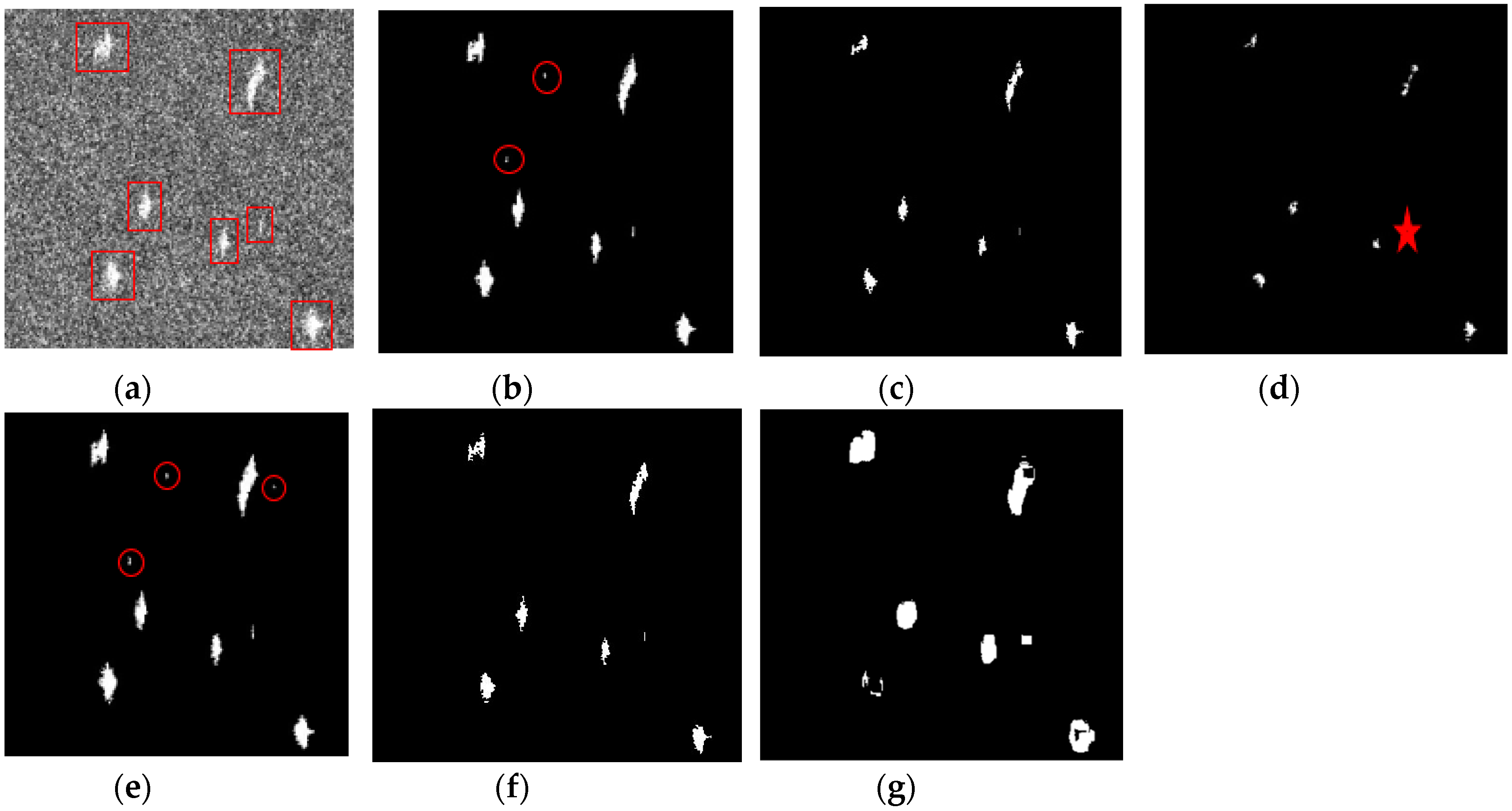
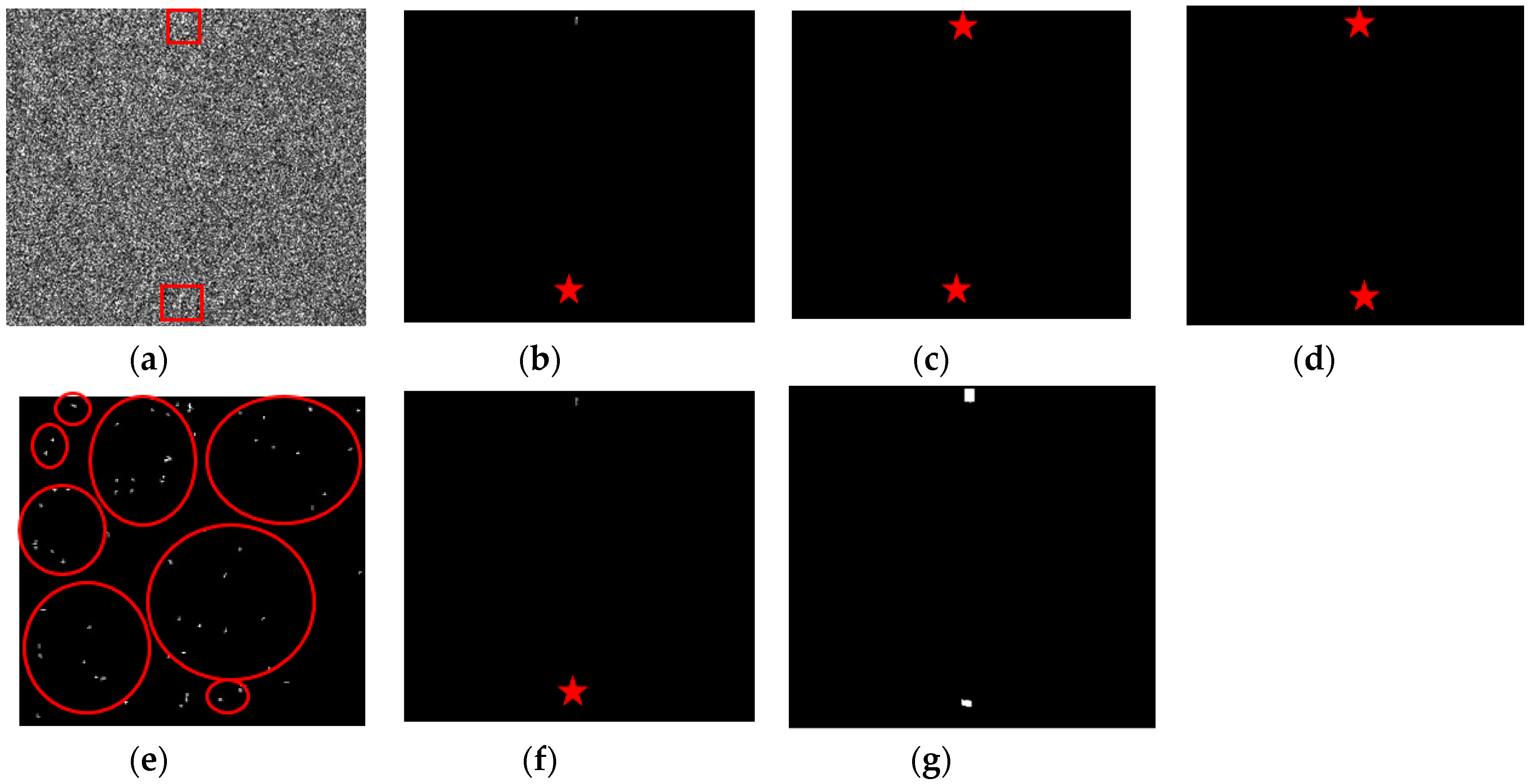
Figure 12, Figure 13 and Figure 14 show three examples of detection results in low, medium and high sea states respectively. In Figure 12, Figure 13 and Figure 14, (b)–(g) are the ship detection results of the Weibull-CFAR, Log-normal-CFAR, G⁰-CFAR, K-CFAR, GГD-CFAR and phase factor detectors. The red boxes and red circles represent ships matched with AIS and false alarms respectively, and the red stars represent ships undetected. In Figure 12 (low sea state), the Weibull-CFAR, K-CFAR and phase factor detectors are the best without false alarms or missing ships, while a ship is missing in Log-normal-CFAR and GГD-CFAR detection, what’s worse, two ships are missing in G⁰-CFAR detection.

In Figure 13 (medium sea state), the Log-normal-CFAR, GГD-CFAR and phase factor detectors perform better than the other detectors. Two and three false alarms exist in Weibull-CFAR and K-CFAR respectively, and a ship in G⁰-CFAR is failed to be detected.

In Figure 14 (high sea state), only the phase factor detector detects two ships without any false alarm. Weibull-CFAR, GГD-CFAR, Log-normal-CFAR and G⁰-CFAR missing one or two ships, and K-CFAR detected all ships but with too many false alarms. The results indicate that the CFAR method is not stable in different conditions, easily causing false alarms and missing detection. In general, the phase factor performs better than the other detectors even in high sea state, while the detection performance of the Weibull-CFAR, Log-normal-CFAR, G⁰-CFAR, K-CFAR and GГD-CFAR decrease with the increasing sea state. The results are in accordance with the theory presented in Section 4.4.

6. Conclusions

In this paper, in order to establish a reliable feature selection method for marine vessel monitoring purposes, CP and DP SAR data were simulated by five FP RADARSAT-2 images, and forty features were extracted from the FP, CP and DP decomposition. We comprehensively quantified and evaluated these features for ship detection by using the Euclidean distance. The result indicated that features f7, f9, f11, c4, c5, c6, c11, c12, c15 and d5 perform better than the other features. For features selected by the Euclidean distance, the relevance between ships and features, along with the redundancy among different features, are further analyzed. The ship detection performance of f7, f9, f11, c4, c5, c6, c11, c12, c15 and d5 from the mutual information are consistent with those from the Euclidean distance. Furthermore, the mutual information among the features f7, f9, f11, c4, c5, c6, c11, c12, c15 and d5 are low. In conclusion, f11, c4, c6, c11 and c12 are used for ship detection, which indicates that the features’ performance in CP SAR mode is better than that in DP and FP SAR mode.

The features in CP SAR mode are further studied to present a new feature that is simple and suitable for use in complex sea states for ship detection. After a series of derivations and analyses by introducing the sea surface roughness, a new feature, named the phase factor, is proposed that can discriminate the ships and sea surface by a constant 0 and is simpler than the CFAR method without the need for false alarm setting and complex threshold calculations by using a segmentation algorithm. What’s more, it is independent of the sea surface roughness and can achieve good performance even in a high sea state.

Experiments demonstrate that the phase factor is stable and better than the roundness, delta, HESA and CFAR detectors in low, medium and high sea states. The performances of the phase factor, roundness, delta, and the HESA are 65, 54, 41 and 9 times that of the amplitude of RV polarization, respectively. In comparison with CFAR method, the phase factor detector is best in low (FOM: 0.94), medium (FOM: 1) and high sea states (FOM: 0.86) for ship detection, followed by Weibull-CFAR, Log-normal-CFAR and GГD-CFAR, while G⁰-CFAR and K-CFAR are the worst, which is caused by high false alarms, low correct detection rates, or both. Therefore, the phase factor can be used in complex sea states for ship detection, especially for the detection of weak and small ship targets in a high sea state.

References

- Nicolas, J.M.; Anfinsen, S.N. Introduction to second kind statistics: Application of log-moments and log-cumulants to the analysis of radar image distributions. Trait. Signal 2002, 19, 139–167. [Google Scholar]
- Ai, J.; Qi, X.; Yu, W.; Yu, W.; Deng, Y.; Liu, F.; Shi, L. A new CFAR ship detection algorithm based on 2-D joint log-normal distribution in SAR images. IEEE Geosci. Remote Sens. Lett. 2010, 7, 806–810. [Google Scholar] [CrossRef]
- Qin, X.; Zhou, S.; Zou, H.; Gao, G. A CFAR detection algorithm for generalized gamma distributed background in high-resolution SAR images. IEEE Geosci. Remote Sens. Lett. 2012, 10, 806–810. [Google Scholar]
- Angelliaume, S.; Rosenberg, L.; Ritchie, M. Modeling the Amplitude Distribution of Radar Sea Clutter. Remote Sens. 2019, 11, 319. [Google Scholar] [CrossRef]
- He, Z.; Zhou, X.G.; Lu, J.; Kuang, G.Y. A fast CFAR detection algorithm based on the G0 distribution for SAR images. J. Natl. Univ. Def. Technol. 2009, 31, 47–51. [Google Scholar]
- Mahdianpari, M.; Salehi, B.; Mohammadimanesh, F.; Brisco, B. An assessment of simulated compact polarimetric SAR data for wetland classification using random forest algorithm. Can. J. Remote Sens. 2017, 43, 468–484. [Google Scholar] [CrossRef]
- Ouchi, K. Recent Trend and Advance of Synthetic Aperture Radar with Selected Topics. Remote Sens. 2013, 5, 716–807. [Google Scholar] [CrossRef] [Green Version]
- Mazzarella, F.; Vespe, M.; Santamaria, C. SAR ship detection and self-reporting data fusion based on traffic knowledge. IEEE Geosci. Remote Sens. Lett. 2015, 12, 1685–1689. [Google Scholar] [CrossRef]
- Sun, Y.; Wang, C.; Zhang, H.; Wu, F.; Zhang, B. A new PolSAR ship detector on RADARSAT-2 data. Proc. SPIE 2012, 8525. [Google Scholar] [CrossRef]
- Sugimoto, M.; Ouchi, K.; Nakamura, Y. On the novel use of model-based decomposition in SAR polarimetry for target detection on the sea. Remote Sens. Lett. 2013, 4, 843–852. [Google Scholar] [CrossRef]
- Shirvany, R.; Chabert, M.; Tourneret, J.Y. Ship and oil-spill detection using the degree of polarization in linear and hybrid/compact dual-pol SAR. IEEE J. Sel. Top. Appl. Earth Observ. Remote Sens. 2012, 5, 885–892. [Google Scholar] [CrossRef]
- Touzi, R.; Vachon, P.W. RCM polarimetric SAR for enhanced ship detection and classification. Can. J. Remote Sens. 2015, 41, 473–484. [Google Scholar] [CrossRef]
- Yin, J.; Yang, J. Ship detection by using the M-Chi and M-Delta decomposition. In Proceedings of the 2014 IEEE Geoscience and Remote Sensing Symposium, Quebec City, QC, Canada, 13–18 July 2014. [Google Scholar]
- Yin, J.; Yang, J.; Zhou, Z.S.; Song, J. The Extended Bragg Scattering Model-Based Method for Ship and Oil-Spill Observation Using Compact Polarimetric SAR. IEEE J. Sel. Top. Appl. Earth Observ. 2015, 8, 3760–3772. [Google Scholar] [CrossRef]
- Paes, R.L.; Nunziata, F.; Migliaccio, M. On the capability of hybrid-polarity features to observe metallic targets at sea. IEEE J. Ocean. Eng. 2016, 41, 346–361. [Google Scholar] [CrossRef]
- Gao, G.; Gao, S.; He, J.; Li, G. Adaptive Ship Detection in Hybrid-Polarimetric SAR Images Based on the Power-Entropy Decomposition. IEEE Trans. Geosci. Remote Sens. 2018, 56, 5394–5407. [Google Scholar] [CrossRef]
- Buono, A.; Nunziata, F.; Migliaccio, M. Analysis of full and compact polarimetric SAR features over the sea surface. IEEE Geosci. Remote Sens. Lett. 2016, 13, 1527–1531. [Google Scholar] [CrossRef]
- Charbonneau, F.J.; Brisco, B.; Raney, R.K.; McNairn, H.; Liu, C.; Vachon, P.W.; Geldsetzer, T. Compact polarimetry overview and applications assessment. Can. J. Remote Sens. 2010, 36, S298–S315. [Google Scholar] [CrossRef]
- Buono, A.; Nunziata, F.; Migliaccio, M. Polarimetric analysis of compact-polarimetry SAR architectures for sea oil slick observation. IEEE Trans. Geosci. Remote Sens. 2016, 54, 5862–5874. [Google Scholar] [CrossRef]
- Souyris, J.C.; Imbo, P.; Fjortoft, R. Compact polarimetry based on symmetry properties of geophysical media: The/spl pi//4 mode. IEEE Trans. Geosci. Remote Sens. 2005, 43, 634–646. [Google Scholar] [CrossRef]
- Raney, R.K. Comparing compact and quadrature polarimetric SAR performance. IEEE Geosci. Remote Sens. Lett. 2016, 13, 861–864. [Google Scholar] [CrossRef]
- Gao, G.; Gao, S.; He, J. Ship Detection Using Compact Polarimetric SAR Based on the Notch Filter. IEEE Trans. Geosci. Remote Sens. 2018, 56, 5380–5393. [Google Scholar] [CrossRef]
- Hajnsek, I.; Pottier, E.; Cloude, S.R. Inversion of surface parameters from polarimetric SAR. IEEE Trans. Geosci. Remote Sens. 2003, 41, 727–744. [Google Scholar] [CrossRef]
- Hersbach, H. CMOD5: An Improved Geophysical Model Function for ERS C-Band Scatterometry; European Centre for Medium-Range Weather Forecasts: Reading, UK, 2003. [Google Scholar]
- Hersbach, H.; Stoffelen, A.; deHaan, S. An improved C-band scatterometer ocean geophysical model function: CMOD5. J. Geophys. Res. Oceans 2007, 112. [Google Scholar] [CrossRef]
- Beaufort_Scale. Available online: https://en.wikipedia.org/wiki/Beaufort_scale (accessed on 20 May 2018).
- Harati-Mokhtari, A.; Wall, A.; Brooks, P.; Wang, J. Automatic Identification System (AIS): Data reliability and human error implications. J. Navig. 2007, 60, 373–389. [Google Scholar] [CrossRef]
- Tetreault, B.J. Use of the Automatic Identification System (AIS) for maritime domain awareness (MDA). In Proceedings of the OCEANS 2005 MTS/IEEE, Washington, DC, USA, 18–23 Septmber 2005. [Google Scholar]
- Cloude, S.R.; Pottier, E. An entropy based classification scheme for land applications of polarimetric SAR. IEEE Trans. Geosci. Remote Sens. 1997, 35, 68–78. [Google Scholar] [CrossRef]
- Sabry, R.; Ainsworth, T.L. SAR Compact Polarimetry for Change Detection and Characterization. IEEE J. Sel. Top. Appl. Earth Observ. Remote Sens. 2019, 12, 898–909. [Google Scholar] [CrossRef]
- Freeman, A.; Durden, S.L. A three-component scattering model for polarimetric SAR data. IEEE Trans. Geosci. Remote Sens. 1998, 36, 963–973. [Google Scholar] [CrossRef] [Green Version]
- Yamaguchi, Y.; Sato, A.; Boerner, W.M.; Sato, R.; Yamada, H. Four-component scattering power decomposition with rotation of coherency matrix. IEEE Trans. Geosci. Remote Sens. 2011, 49, 2251–2258. [Google Scholar] [CrossRef]
- Yamaguchi, Y.; Moriyama, T.; Ishido, M.; Yamada, H. Four-component scattering model for polarimetric SAR image decomposition. IEEE Trans. Geosci. Remote Sens. 2005, 43, 1699–1706. [Google Scholar] [CrossRef]
- Raney, R.K. Hybrid-polarity SAR architecture. IEEE Trans. Geosci. Remote Sens. 2007, 45, 3397–3404. [Google Scholar] [CrossRef]
- Espeseth, M.M.; Skrunes, S.; Jones, C.E.; Brekke, C.; Holt, B.; Doulgeris, A.P. Analysis of evolving oil spills in full-polarimetric and hybrid-polarity SAR. IEEE Trans. Geosci. Remote Sens. 2017, 55, 4190–4210. [Google Scholar] [CrossRef]
- Nord, M.E.; Ainsworth, T.L.; Lee, J.S.; Stacy, N.J. Comparison of compact polarimetric synthetic aperture radar modes. IEEE Trans. Geosci. Remote Sens. 2009, 47, 174–188. [Google Scholar] [CrossRef]
- Cloude, S.R.; Goodenough, D.G.; Chen, H. Compact decomposition theory. IEEE Geosci. Remote Sens. Lett. 2011, 9, 28–32. [Google Scholar] [CrossRef]
- Raney, R.K.; Cahill, J.T.; Patterson, G.W.; Bussey, D.B.J. The m-chi decomposition of hybrid dual-polarimetric radar data with application to lunar craters. J. Geophys. Res. Planets 2012, 117, E12. [Google Scholar] [CrossRef]
- Shan, Z.; Wang, C.; Zhang, H.; Chen, J. H-Alpha Decomposition and Alternative Parameters for Dual Polarization SAR Data. In Proceedings of the PIERS, SuZhou, China, 12–16 September 2011. [Google Scholar]
- Cloude, S.R. Dual-versus quad-pol: A new test statistic for radar polarimetry. In Proceedings of the PolInSAR Conference—ESAESRIN, Frascati, Italy, 28 January–1 February 2009. [Google Scholar]
- Cao, C.H.; Zhang, J.; Zhang, X. The analysis of ship target detection performance with C band compact polarimetric SAR. Period. Ocean Univ. China 2017, 47, 85–93. [Google Scholar]
- Peng, H.; Long, F.; Ding, C. Feature selection based on mutual information: Criteria of max-dependency, max-relevance, and min-redundancy. IEEE Trans. Pattern Anal. Mach. Intell. 2005, 27, 1226–1238. [Google Scholar] [CrossRef]
- Estévez, P.A.; Tesmer, M.; Perez, C.A.; Zurada, J.M. Normalized mutual information feature selection. IEEE Trans. Neural Netw. 2009, 20, 189–201. [Google Scholar] [CrossRef]
- Bi, N.; Tan, J.; Lai, J.H.; Suen, C.Y. High-dimensional supervised feature selection via optimized kernel mutual information. Expert Syst. Appl. 2018, 108, 81–95. [Google Scholar] [CrossRef]
- Dabboor, M.; Geldsetzer, T. Towards sea ice classification using simulated RADARSAT Constellation Mission compact polarimetric SAR imagery. Remote Sens. Environ. 2014, 140, 189–195. [Google Scholar] [CrossRef]
- Wang, H.; Zhou, Z.; Turnbull, J. Three-Component Decomposition Based on Stokes Vector for Compact Polarimetric SAR. Sensors 2015, 15, 24087–24108. [Google Scholar] [CrossRef]
- Van Zyl, J.J. Unsupervised classification of scattering behavior using radar polarimetry data. IEEE Trans. Geosci. Remote Sens. 1989, 27, 36–45. [Google Scholar] [CrossRef]
- Zhang, X.; Zhang, J.; Meng, J.M.; Chen, L.M. A novel polarimetric SAR ship detection filter. In Proceedings of the IET International Radar Conference 2013, Xi’an, China, 14–16 April 2013. [Google Scholar]
Figure 1.
The main parts of this paper.
Figure 2.
The RGB images of Scenes 01–05 after geometric correction. R = HH, G = HV, B = VH. (a) Scene 01: areas of the West Lamma Channel in Hong Kong; (b) scene 02: areas of the Yangtze Estuary; (c) scene 03: areas of the Yellow River Estuary; (d) scene 04: areas of Lianyungang; (e) scene 05: areas of Singapore.
Figure 3.
Matching results of a SAR image and the AIS.
Figure 4.
Euclidean distance between ships and the sea area in five images.
Figure 5.
Normalized mutual information among different features, and samples are from scene 01 (a) and scene 03 (b).
Figure 6.
Three examples of the values of ships and the sea surface in the roundness. (a) Area in the red box from scene 01. (b) Area in the red box from scene 02. (c) Area in the red box from scene 05.
Figure 7.
Three examples of the values of ships and the sea surface in the delta. (a) Area in the red box from scene 01. (b) Area in the red box from scene 02. (c) Area in the red box from scene 05.
Figure 8.
Three examples of the values of ships and the sea surface in the HESA. (a) Area in the red box from scene 01. (b) Area in the red box from scene 02. (c) Area in the red box from scene 05.
Figure 9.
Three examples of the values of ships and the sea surface in the phase factor. (a) Area in the red box from scene 01. (b) Area in the red box from scene 02. (c) Area in the red box from scene 05.
Figure 10.
Comparison of the five detectors in a medium sea state. (a) Amplitude of RV polarization. (b) Roundness. (c) Delta. (d) HESA. (e) Phase factor. (f) 3-D display of amplitude. (g) 3-D display of roundness. (h) 3-D display of delta. (i) 3-D display of HESA. (j) 3-D display of phase factor.
Figure 11.
Comparison of the five detectors in a high sea state. (a) Amplitude of RV polarization; (b) Roundness; (c) Delta; (d) HESA; (e) Phase factor; (f) 3-D display of the amplitude; (g) 3-D display of roundness; (h) 3-D display of delta; (i) 3-D display of HESA; (j) 3-D display of phase factor.
Figure 12.
Detection performance comparison of CFAR and phase factor detectors in a low sea state. (a) Amplitude of RV polarization; (b) Weibull-CFAR; (c) Log-normal-CFAR; (d) G0-CFAR; (e) K-CFAR; (f) GГD-CFAR; (g) phase factor detector.
Figure 13.
Detection performance comparison of CFAR and phase factor detectors in a medium sea state. (a) Amplitude of RV polarization; (b) Weibull-CFAR; (c) Log-normal-CFAR; (d) G0-CFAR; (e) K-CFAR; (f) GГD-CFAR; (g) phase factor detector.
Figure 14.
Detection performance comparison of CFAR and phase factor detectors in a high sea state. (a) Amplitude of RV polarization; (b) Weibull-CFAR; (c) Log-normal-CFAR; (d) G0-CFAR; (e) K-CFAR; (f) GГD-CFAR; (g) phase factor detector.