Landslide Deformation Monitoring by Adaptive Distributed Scatterer Interferometric Synthetic Aperture Radar

MOE Collaborative Innovation Center of Spatial Information Technology for High-speed Railway Safety & State-Province Joint Engineering Laboratory of Spatial Information Technology for High-Speed Railway Safety, Southwest Jiaotong University, Chengdu 611756, China
*
Author to whom correspondence should be addressed.
Remote Sens. 2019, 11(19), 2273; https://0-doi-org.brum.beds.ac.uk/10.3390/rs11192273
Submission received: 16 August 2019
/
Revised: 26 September 2019
/
Accepted: 26 September 2019
/
Published: 29 September 2019
(This article belongs to the Special Issue Global Geospatial Information and Hazards Management for Smart Environments)
Abstract
:Landslide is the second most frequent geological disaster after earthquake, which causes a large number of casualties and economic losses every year. China frequently experiences devastating landslides in mountainous areas. Interferometric Synthetic Aperture Radar (InSAR) technology has great potential for detecting potentially unstable landslides across wide areas and can monitor surface displacement of a single landslide. However traditional time series InSAR technology such as persistent scatterer interferometry (PSI) and small-baseline subset (SBAS) cannot identify enough points in mountainous areas because of dense vegetation and steep terrain. In order to improve the accuracy of landslide hazard detection and the reliability of landslide deformation monitoring in areas lacking high coherence stability point targets, this study proposes an adaptive distributed scatterer interferometric synthetic aperture radar (ADS-InSAR) method based on the spatiotemporal coherence of the distributed scatterer (DS), which automatically adjusts its detection threshold to improve the spatial distribution density and reliability of DS detection in the landslide area. After time series network modeling and deformation calculation of the ADS target, the displacement deformation of the landslide area can be accurately extracted. Shuibuya Town in Enshi Prefecture, Hubei Province, China, was used as a case study, along with 18 Sentinal-1A images acquired from March 2016 to April 2017. The ADS-InSAR method was used to obtain regional deformation data. The deformation time series was combined with hydrometeorological and related data to analyze landslide deformation. The results show that the ADS-InSAR method can effectively improve the density of DS distribution, successfully detect existing ancient landslide groups and determine multiple potential landslide areas, enabling early warning for landslide hazards. This study verifies the reliability and accuracy of ADS-InSAR for landslide disaster prevention and mitigation.
1. Introduction
Landslides are a common geological disaster typically induced by persistent heavy rainfall, human activities and earthquakes. Landslides are extremely destructive; they severely restrict the economic development of countries around the world and pose a serious threat to local public safety [1]. Monitoring and analysis of the landslide deformation area can provide an important basis for landslide early warnings; therefore, this is key research area for geological disaster prevention and mitigation.
At present, international landslide monitoring methods predominantly include absolute deformation measurements based on global positioning systems (GPS), electronic total stations, levels and so forth [2,3,4], relative deformation measurements based on displacement meters, crack meters or fiber sensors and so forth [5,6] and quantitative analysis based on light detection and ranging (LIDAR) technology [7,8]. Although these methods, which are based on ground point observations, have the advantage of high precision, the number of monitoring points on the landslide body is limited by the large amounts of field work and economic costs involved. The density of monitoring points is typically low; thus, it is difficult to capture the spatial details of landslide deformation. As a result, these methods cannot identify the distribution of large-scale landslide groups and their dynamic evolution.
In recent years, interferometric synthetic aperture radar (InSAR) remote sensing has shown excellent application prospects for monitoring large-scale deformation (including landslide displacement) [9,10,11] and has been used to monitor earthquakes, glaciers and volcanoes and achieved good results [12]. In order to improve the practicality of InSAR techniques, Ferretti, Berardino, Hopper et al. [13,14,15] have proposed multi-temporal InSAR (MTInSAR) to reduce the atmospheric delays and spatiotemporal decorrelation. For instance, Lei et al. [16] applied the PS-InSAR method to ERS-1/2, Radarsat-1 and TerraSAR-X images between 1992 and 2010, revealing the velocity and locating landslides areas of Berkeley hills landslides. Zhao et al. [17] monitored the landslide along the Jinsha River by using 20 advanced land observation satellite (ALOS)/phased arrey type L-band synthetic aperture radar (PALSAR) images with the small baseline subset (SBAS) InSAR technique. However this technique needs more persistent scatterers (PSs) while there are fewer persistent scatterer (PS) targets due to general vegetation cover that forms on the landslide body in mountainous areas. distributed scatterer (DS) interferometry can overcome the problem of no PS targets in the landslide area and greatly increase the detection of effective deformation monitoring points [18]. However, for the mountain areas, there are differences in the spatiotemporal coherence of the target due to regional differences in mountainous areas. If the global threshold method is still adopted, low quality DS may be selected and high quality DS may be deleted.
In order to improve the spatial resolution and success rate of large-scale landslide hazard detection and landslide displacement monitoring, an adaptive distributed scatterer InSAR (ADS-InSAR) method is proposed. This method automatically adjusts the DS target detection threshold according to the spatiotemporal coherence of different distributed targets, thereby improving the spatial distribution density and reliability of DS detection in landslide areas. The adaptive distributed scatterer (ADS) target is subjected to time series network modeling and deformation solution calculation to extract the displacement deformation of the landslide area. In order to verify the validity and reliability of this method, this study uses Shuibuya Town in Hubei Province, China, as the research area. 18 C-band Sentinel-1A images are employed to detect the spatial distribution of landslide points in the area and extract and analyze surface deformation data.
2. Adaptive Distributed Scatterer InSAR Method
Compared with the conventional DS-InSAR method, ADS-InSAR uses the fast statistically homogenous point (SHP) selection method to identify and derivate SHP. It converts the hypothesis test problem into a confidence interval estimate to set the appropriate SHP number threshold, then divide pixel targets above the threshold into DS candidate (DSC) points. After that, the image is divided into high and low coherence regions according to coherence and the adaptive coherence threshold is set to obtain the final DS candidate points. Finally, the parameters of the DS target are solved to obtain the final deformation result.
2.1. ADS Target Recognition and Detection
The parameter p is set as a point to be evaluated, whose N time intensity samples are {a1, a2, …, aN}. Then, the sample point estimate of expectation of p is a(p) = (a1(p) + a2(p) + … + aN(p))/N. To find the interval estimate of μ(p), we first need to determine the distribution of a(p). According to the central limit theorem, a(p) gradually approaches a Gaussian distribution as the number of samples N increases. If the number of samples N is large enough, the Gaussian assumption can be satisfied. At this time, the interval estimation of a(p) is:
where P{·} represents the probability, Var(a(p)) is the true variance of point p and z1−α/2 is the corresponding 1 − α/2 point in the standard normal distribution. According to the statistical theory of SAR images, the single-view intensity image in the homogeneous region obeys the Rayleigh Distribution [19]. The coefficient of variation CV is constant:
Here, E(∙) represents the expectation. We assume that the samples are homogeneous in temporal space, when the backscattering characteristics are not very strong. Then, Equation (1) can be converted to:
In actual processing, it is first assumed that the sample expectation and the true value are approximately equal. By calculating the sample mean of all pixels except the reference cell and comparing them to Equation (3), all points where the sample mean falls within the interval can be considered as homogenous. However, when the number of time samples is small, there is a large uncertainty in the mathematical expectation of the obtained samples. For this reason, in order to reduce the estimated deviation caused by the distribution tail, the value of α is generally set to 50%. Subsequently, the samples of the pixels within the set are averaged, the sample expectation is re-estimated and the re-estimated expectation is considered as the true mean of the reference points. By iterating through the above steps and decreasing the alpha value to increase the interval range, a set of points that meet the requirements is obtained. After further screening to retain the point of excellent adjacency, the points are considered SHP [21]. It should be noted that, in order to ensure the accuracy of the solution results and the validity of the interval estimation, determination of the N value is very important. According to the classical statistical literature, when the probability distribution is smooth (just like single-view intensity images subject to Rayleigh Distribution) that N = 5 is close enough to the Gaussian distribution [22].
After determining the SHP of each pixel through the method of fast statistically homogenous point selection, it is necessary to obtain the SHP number threshold to determine whether it is a DSC; that is, when the SHP number is greater than the given threshold (generally set as the average of all SHP Numbers), the point is considered as a DSC. After obtaining the DSC, the image is adaptively filtered. The principle of filtering is to improve the coherence of alternative points and remove the majority of speckle noise in the image. The coherence coefficient value of each point is then calculated, which can be obtained by the following estimators [23]:
where is the coherence coefficient value, s1(∙) and s2(∙) represent the single look complex (SLC) image of two scenes used for interference and L represents the number of identical particles in the set.
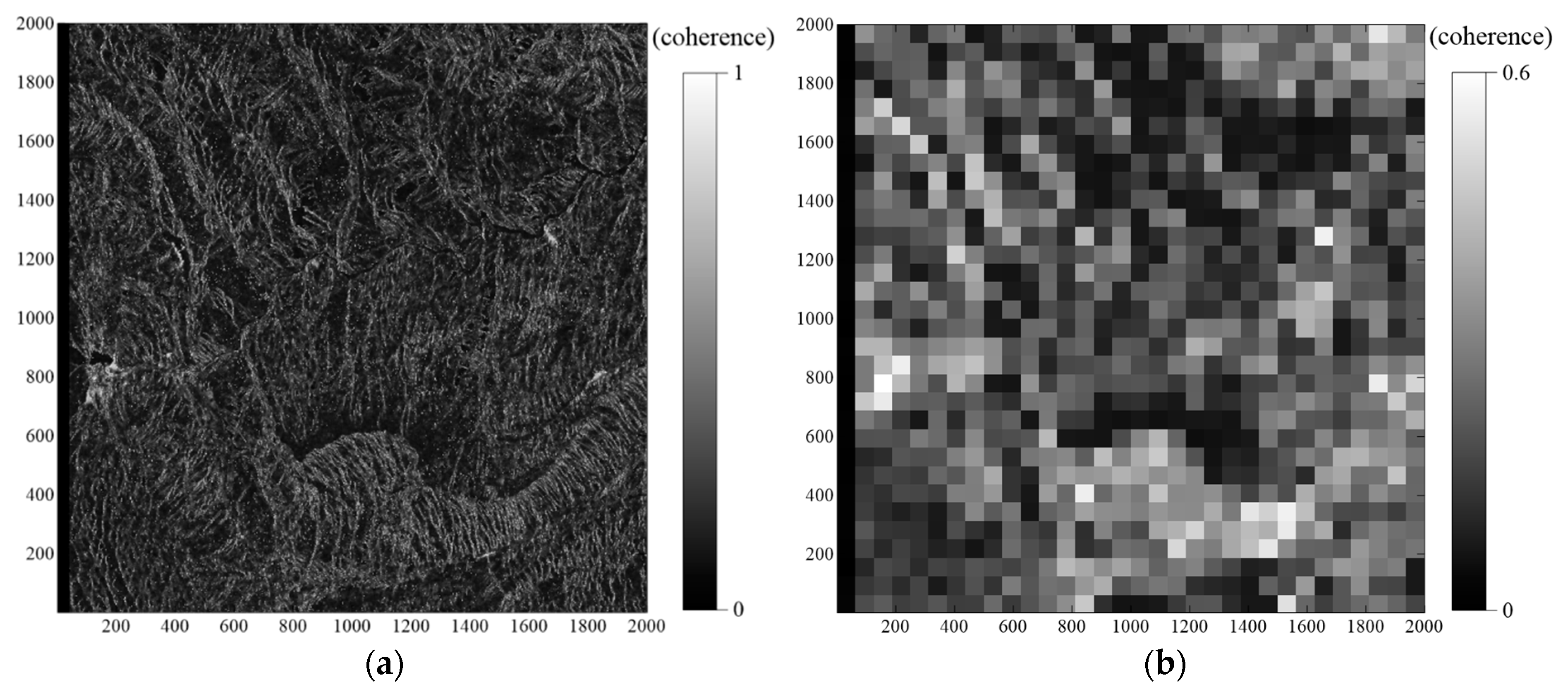
Subsequently, the image region is divided into uniform blocks and the adaptive coherence threshold is calculated by comparing the average coherence coefficient in the block with the overall coherence coefficient of the image. If the average coherence value in the block is greater than the overall coherence coefficient value of the image, the latter will be taken as the threshold value and vice versa. The DSC in the block will continue to be screened. This process is repeated until the point is selected to obtain all DS targets.
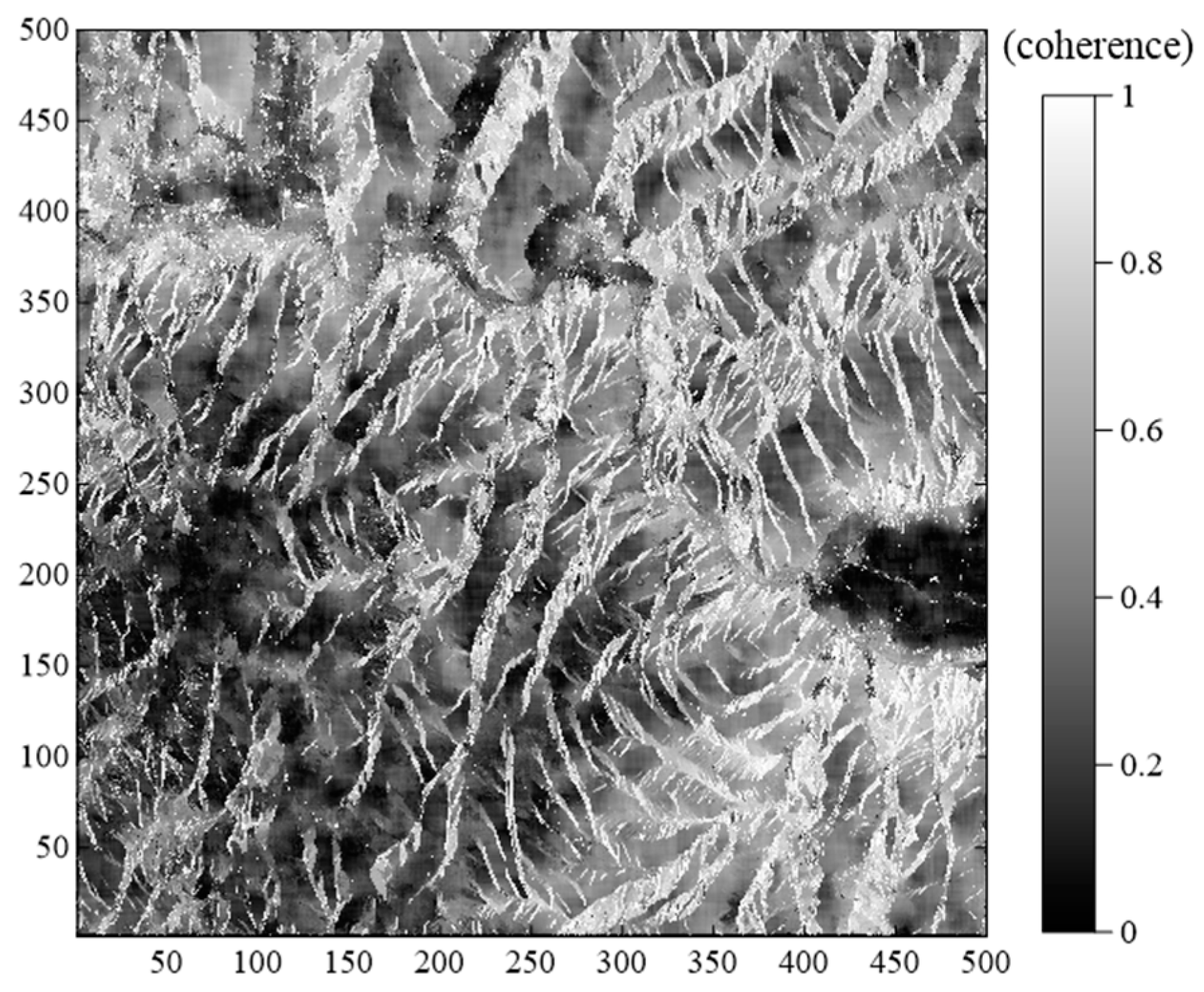
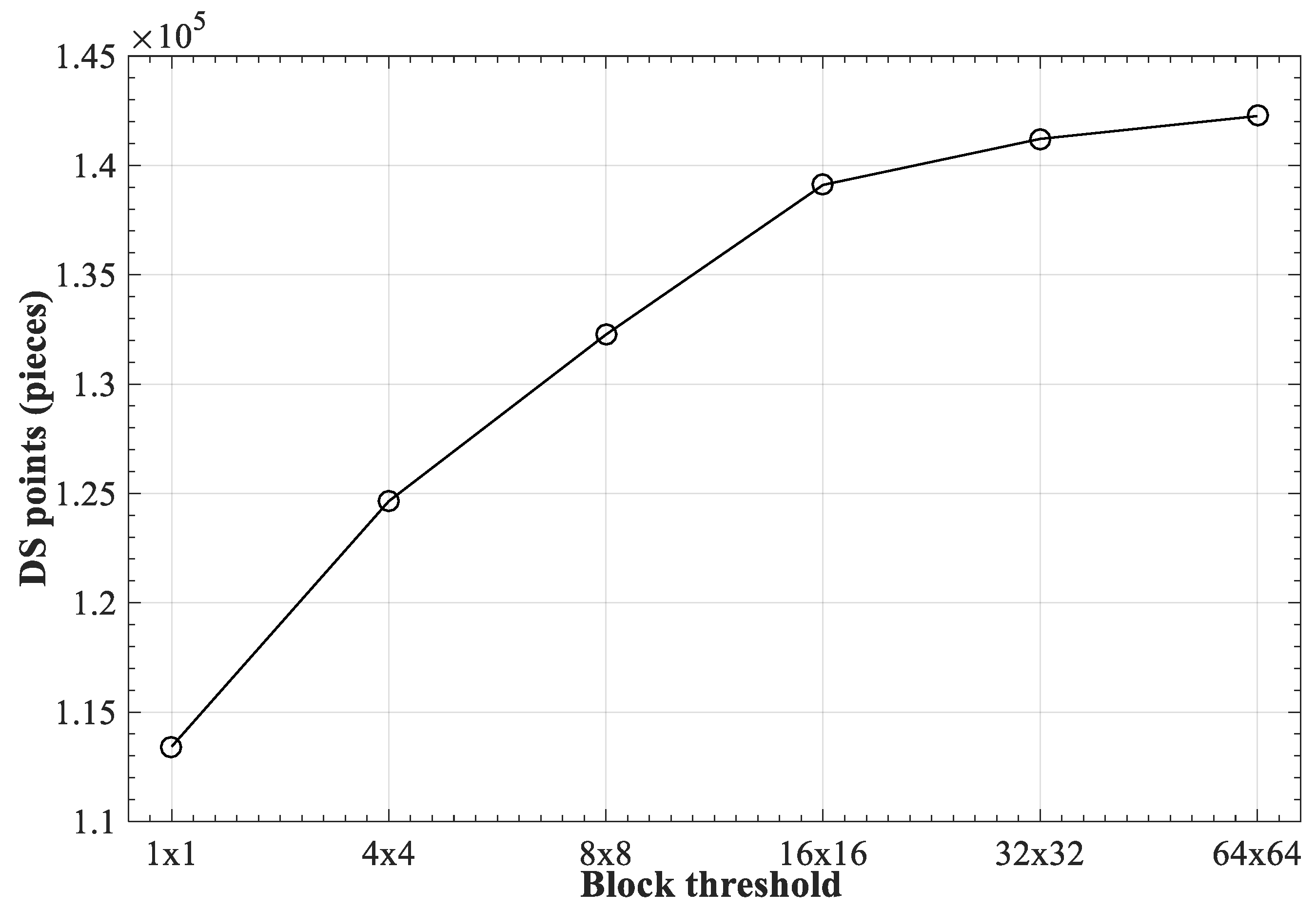
A mountainous area in Yunnan province, southwest China, was selected for the experiment and the regional coherence coefficient is shown in Figure 1. The region was partitioned into 8 × 8, 16 × 16, 32 × 32 and 64 × 64 blocks and the average coherence coefficient value was calculated for each block. The results are shown in Figure 2a–d. The DSC points within the extracted region and the corresponding calculation times are shown in Table 1, the relationship between block threshold and extracted points is shown in Figure 3.
By separating the high and low coherent regions, the adaptive threshold method can further encrypt the highly coherent points in the low coherence regions without losing the highly coherent points in high coherence regions. Experimental results show that, by increasing the set block threshold, the number of extracted DS points starts to increase and eventually becomes stable. Because the computational time of the program should be considered when selecting points in large areas, the threshold value of the partition should not be too large. Therefore, to balance the sufficient number of SHP and the computational time of the program, the 32 × 32 block threshold was chosen as the optimal threshold as it can effectively increase the point density in low coherence regions and strengthen surface feature inversion.
2.2. Parameter Estimation
After all DS point targets are obtained, the three-dimensional phase unwrapping algorithm was used to extract the deformation phase in this experiment. Here “three dimensions” includes two spatial dimensions and one time dimension [24]. Firstly, the phase is unentangled in the time domain and all points in the space are constructed to form a Delaunay triangulation net. Assuming that N SAR images are acquired in the research area over a certain period of time, M interference pairs are formed and their corresponding time baseline is ti (i = 1, 2, …, M) Then, the target x phase of any point in the ith interferogram can be expressed as [25,26]:
The three components on the right of the Equation correspond to the deformation phase, atmospheric phase and noise phase, respectively.
Assuming that deformation in the vertical direction is dominant in the study area, the deformation phase can be expressed as a function of the vertical deformation rate, the time baseline and the incidence angle of radar waves [27]. For N SAR images arranged in time sequence, there are N-1 continuous time intervals (i.e., τ1, τ2, …, τM), which corresponds to the N-1 vertical deformation rate. Therefore, the vector of the vertical deformation rate of a given pixel x can be expressed as:
Assuming that SAR images k and 1 are combined to generate the ith interferogram, the deformation phase in Equation (5) can be expressed as:
where
In Equation (8), β(τj) is:
where λ is the radar signal wavelength (the radar wavelength of the Sentinel-1A satellite is 5.6 cm) and θ is the radar wave incidence angle (the radar wave incidence angle of the Sentinel-1A satellite is approximately 34°). Therefore, Equation (5) can be further expressed as:
where ω(x,ti) is the residual phase, which is the sum of the contribution components of the atmospheric effect and the uncorrelated noise phase. For the ith interferogram, the interference phase increment at any network connection edge of the Delaunay triangulation network (i.e., the arc segment connected by two adjacent point targets x and y) can be expressed as:
where Δω(x,y,ti) is the residual phase increment, which is the sum of the atmospheric effect between two point targets and the phase increment of the uncorrelated noise and ΔVx,y is the increment vector of the vertical deformation rate. For any arc connected by points x and y, M interference pairs can list M Equations as shown in Equation (11) and form the observation Equations [28]. The observation Equations can be expressed by the following matrix:
where A is the coefficient matrix composed of β(τj) and zero values, ΔF is the phase increment vector and W is the residual phase increment. Since the atmospheric phase delay shows the low-frequency characteristics of high correlation in the spatial distribution, high-pass filtering can eliminate the interference phase increment. And the noise phase shows high frequency characteristics in time and space distribution, which can be suppressed by low-pass filtering [29,30]. Then, the least squares adjustment method is adopted to estimate the incremental linear deformation rate, namely:
where ^ is the estimator and Pdd is the prior weight matrix. After the least squares adjustment method is used to estimate the linear deformation rate increment for any arc segment in the point-target network, the phase ambiguity on the arc segment is judged according to the residual phase increment and variance. The arc detected with ambiguity will be removed and is not included in the subsequent deformation analysis. After obtaining the deformation rate increment on the effective arc, taking a certain coherent point as the reference point and using the least squares adjustment method, the vertical deformation rate of all point targets can be obtained [31]. Finally, according to the vertical displacement rate corresponding to different time intervals of each point, the time series displacements of each point can be calculated.
3. Study Area and Data
The research area is located in Hubei province, China and contains Changyang, Badong and Wufeng counties. The mainstream of Qingjiang river flows from west to east across the region. Shuibuya hydropower station is a key hydropower station located on the mainstream. The specific location of the study area is shown in Figure 4.
The region is characterized by undulating mountains, ravines and complex horizontal terrain, typified by karst landforms. The maximum relative height difference is approximately 2900 m and most slopes are covered by vegetation. The formation lithology is mostly shale, which is easily weathered and softened by water [32]. Due to the terrain, the region has four distinct seasons and abundant rainfall. The annual average precipitation reaches 1000 mm. These regional characteristics make the area prone to landslides.
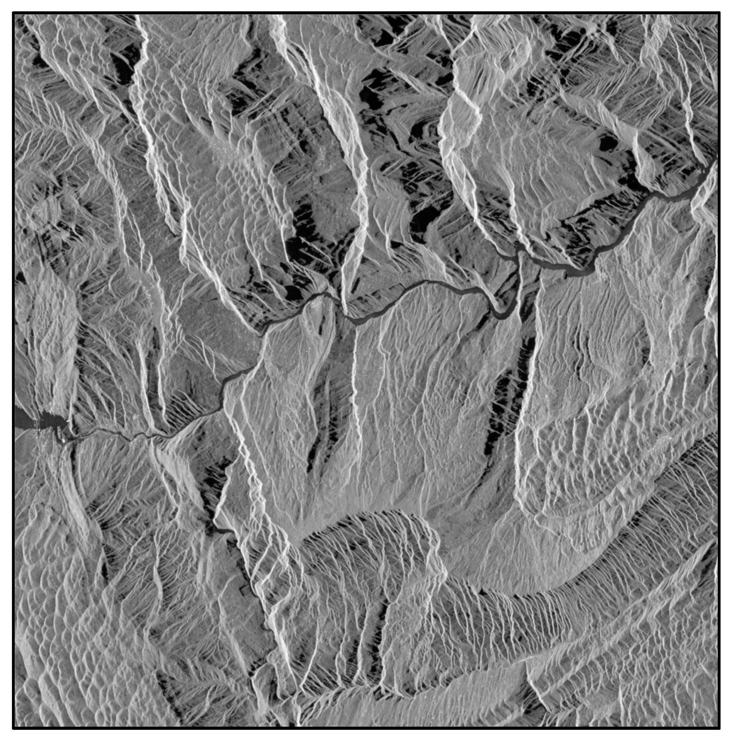
According to historical records, there are several ancient large-scale landslide groups in the study area, with a total volume of 24.2 million m3 and four landslides with volumes over 2 million m3 [33]. Instability related to these landslides will affect internal traffic, the safety of residents and even the stability of the water conservation dam; thus, landslide detection is highly significant in this area. This experiment used 18 Sentinel-1A images (orbital altitude: 693 km, orbital inclination: 98.18°, re-visit period: 12 days, C-band wavelength: 5.6 cm) provided by the European Space Agency (ESA). The image of the average amplitude in the study area is shown in Figure 5. The time period was from March 2016 to April 2017. The minimum time resolution was 13 days and the spatial resolution was 30 m. The elevation data was generated using SRTM1 DEM data provided by the United States Geological Survey (USGS) with a spatial resolution of 30 m.
4. Results
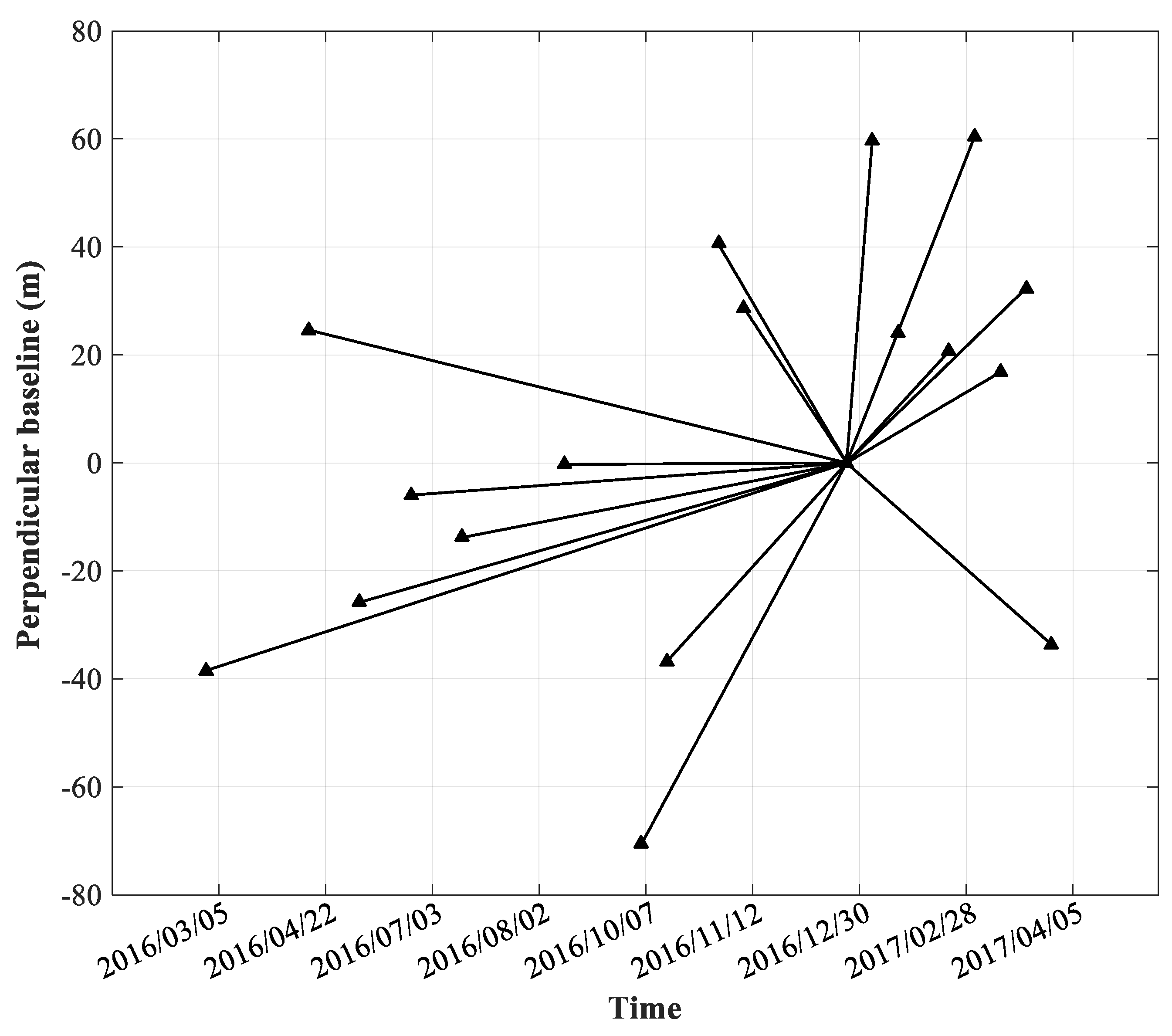
The radar image acquired on 30 December 2016 was used as the single main image in the experiment and all other images were used as auxiliary images to form a total of 17 interference image pairs. The time-space baseline distribution is shown in Figure 6. The interference pattern formed by the 20161230–20160703 interference pair was used as an example (Figure 7). Due to the dense vegetation and smaller artificial surface area, the interference fringes in the interference pattern are sparse and the interference effect is poor.
The fast SHP selection algorithm introduced in Section 2.1 was used to individually select homogenous points for each pixel. The selected window size was set to 15 × 15, the threshold of homogenous point numbers was set as the mean of SHP number 98 and the DS candidate points (DSC) were selected. The coherence of DSC was then estimated and the image was segmented. As mentioned above, considering the computational time of the algorithm, the number of blocks was set to 32 × 32 = 1024. The coherence coefficient diagram and block results are shown in Figure 8. The coherence threshold value of each spatial coordinate was obtained by calculating the mean of the coherence coefficient in each block and the DSC was further analyzed to obtain the DS points. Finally, 287,584 DS points were obtained in the experimental area. In order to compare the advantages of the ADS-InSAR method proposed in this study, the empirical threshold method (DS-InSAR) was also used to select DS points and a total of 157,174 DS points were obtained. The spatial distribution map of DS points for the two methods is shown in Figure 9.
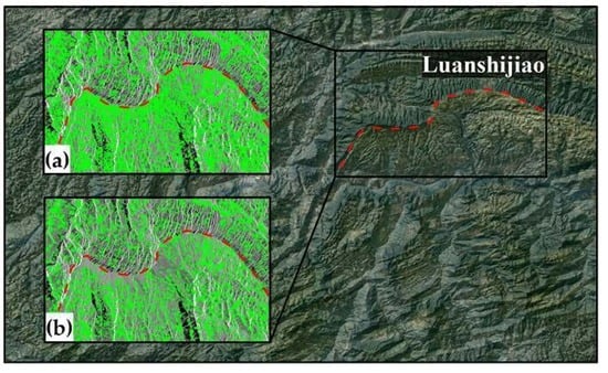
Luanshijiao area, shown in Figure 10, is used as an example; it is densely vegetated and belongs to a low coherence area. In the figure, (a) is the detection point target result of the ADS-InSAR method and (b) is the detection point target result of the DS-InSAR method. By combining the results with the topographic map, it is clear that the area above the red wavy ridgeline is covered by dense vegetation and the number of point targets extracted by the two methods are almost same. And the area below the red wavy ridgeline contain many villages, among which there are many roads and bare lands. Although these features with vegetation coverage may result in a decrease of coherence, they have stable phase in time series and can be scatterer targets. After the adaptive threshold is determined for the ADS-InSAR method, the point targets can be extracted.
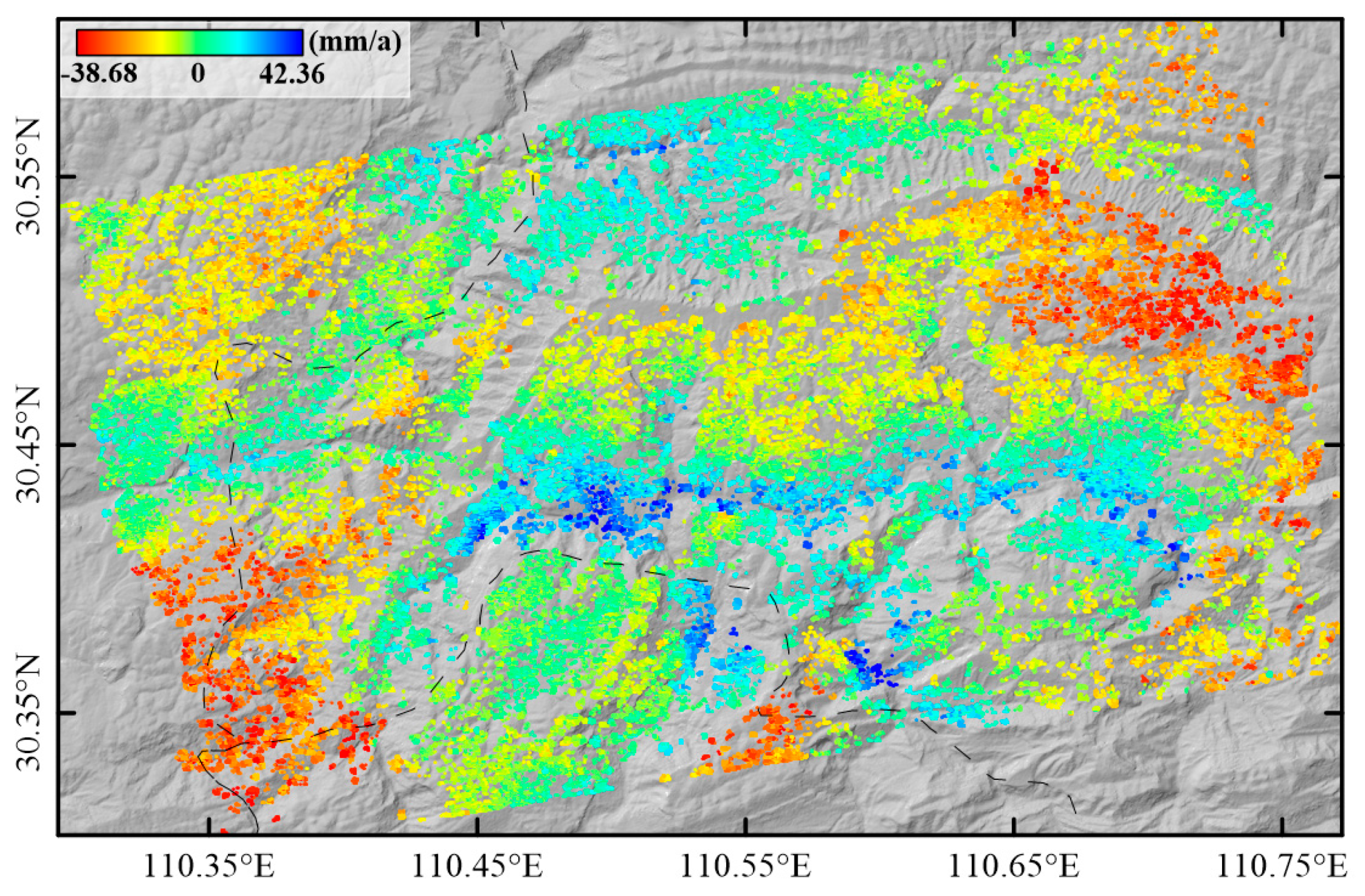
Furthermore, the comparison shows that the DS points selected by the ADS-InSAR method are denser in the low coherence region, which is more conducive to surface deformation inversion. Finally, all the acquired DS targets were used to conduct phase unwrapping with the three-dimensional phase unwrapping algorithm. The annual deformation rate variation interval in the study area was −38.7 mm/a to approximately +46.3 mm/a. The distribution of the annual average settlement rate is shown in Figure 11.
5. Discussion
5.1. Discussion of Landslide Monitoring Results
The results of the regional deformation time sequence are shown in Figure 12. The majority of time points of large-scale deformation in this region are from June 2016 to August 2016. The left part and upper right part of the region shows settlement changes from May 2016, whereas the middle part shows uplift changes. With time, the subsidence and uplift conditions become gradually weaker.
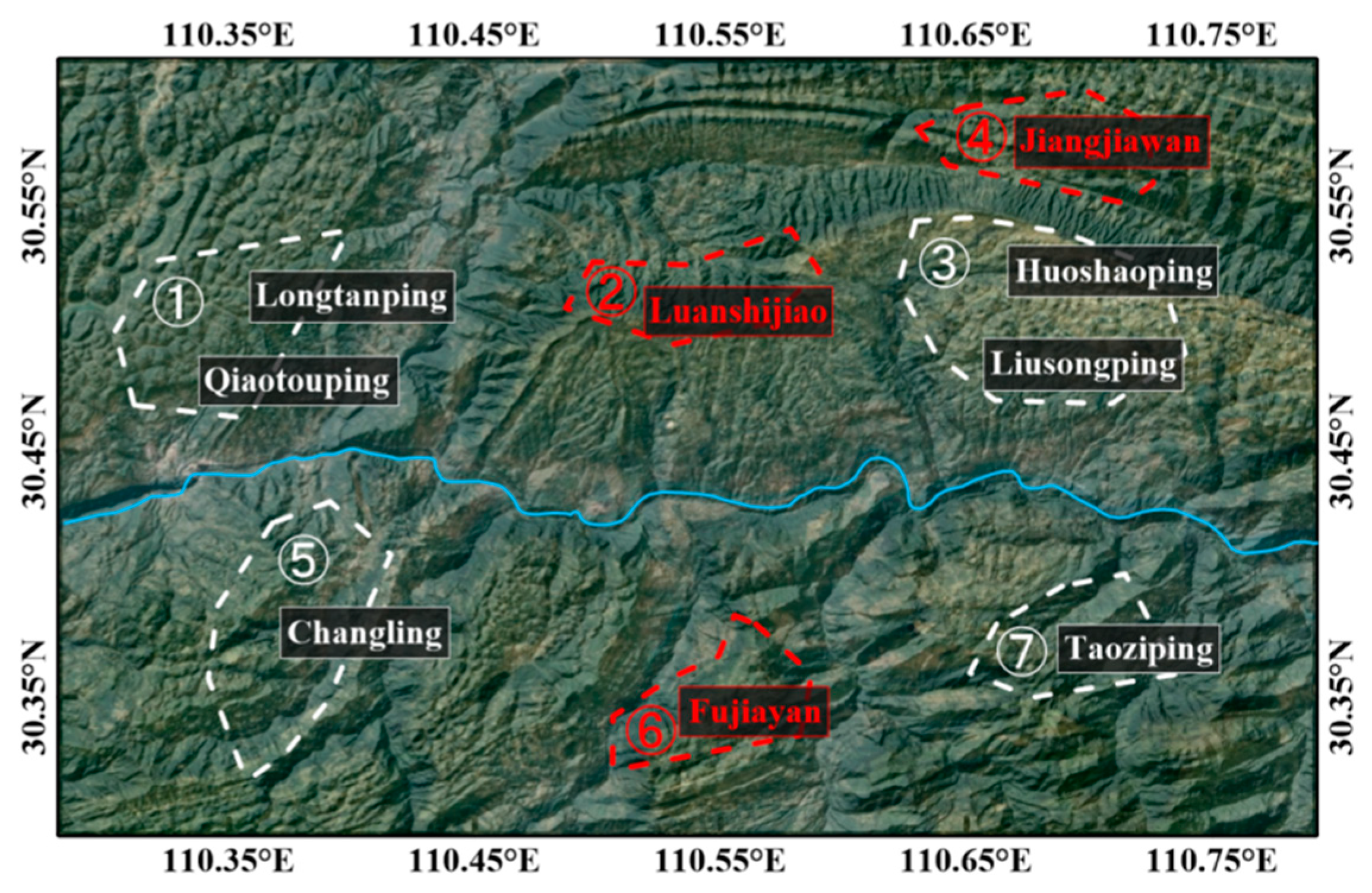
According to the DS average annual deformation rates in Figure 11 and the deformation sequence results in Figure 12, seven suspected landslide areas are detected in the experimental area—zone 1: Longtanping village and Qiaotouping village; zone 2: Luanshijiao area; zone 3: Huoshaoping village and Liusongping village; zone 4: Jiangjiawan village; zone 5: Changling village; zone 6: Fujiayan village; and zone 7: Taoziping village. As shown in Figure 13, the white areas show the confirmed landslide areas and the red areas show suspected landslide areas. Although the suspected landslide areas lack relevant data and evidence, an analysis of local historical data and surrounding environmental factors suggests that some of the landslide points are ancient small-scale landslides and are under continuous monitoring by the relevant departments. Moreover, due to the precipitation and hydropower station discharge caused by the increased groundwater, surface uplift in the experimental area is mainly concentrated in the Qingjiang river basin.
Based on field investigations and relevant data from March 2016 to April 2017, the cause of large-scale settlement has been found. It is predominantly attributed to three major aspects—geological structure, climate change and human factors.
5.1.1. Geological Structure and Lithology
The study area is large and the geological environment is complex. The regional geological structure can be divided into two types. (1) The Changyang county geomorphologic type belongs to structural erosion and a low Zhongshan landscape, the slope body structure type is typically forward slope and the slope is generally 20–40° [34]. (2) The Badong county and Wufeng county landform type belongs to a karst landscape typified by low mountain canyons and dissolution basins. The slope structure is complex and the slope is generally 17–30° [35,36].
For lithology in the study area, it can be approximately divided into three—(1) The Changyang county geomorphologic type belongs to structural erosion. The formation lithology is composed of limestone mixed with shale in the lower Permian Gufeng formation. Shale is prone to wind and bloom, is easily softened in water, has low mechanical strength, experiences large deformation under the influence of external forces and typically exhibits internal displacement under the influence of internal forces [34]; (2) The Badong county landform type belongs to a karst landscape typified by low mountain canyons and dissolution basins. The lithology of the strata is predominantly the Triassic lower Daye formation, Permian lower Dalong formation, Wujiaping formation, Quaternary slope collapse sediments and landslide deposits [35]. The majority of sediments are gray shale with a large amount of debris distributed on the slope surface, which is easily weathered in later stages and easy to soften and muddy when exposed to water; (3) The entire area of Wufeng county is mountainous and belongs to a karst landscape with many karst caves. The terrain slopes gradually from west to east. The stratum lithology is Quaternary artificial accumulation debris and gravel block layers and the upper stratum lithology is loose, easy to percolate and affected by weathering [36].
Although the geological environment varies greatly between different areas, the lithology of the strata is easily weathered and softened by water. Therefore, when heavy rainfall occurs, a large amount of surface water seeps into the rock mass, which reduces adhesion between the rocks and reduces their shear strength. Furthermore, due to softening and muddying, the top of the weak layer becomes looser, the penetrating shear failure surface further deteriorates into a sliding surface and the slope loses stability, leading to a landslide.
5.1.2. Climate Change
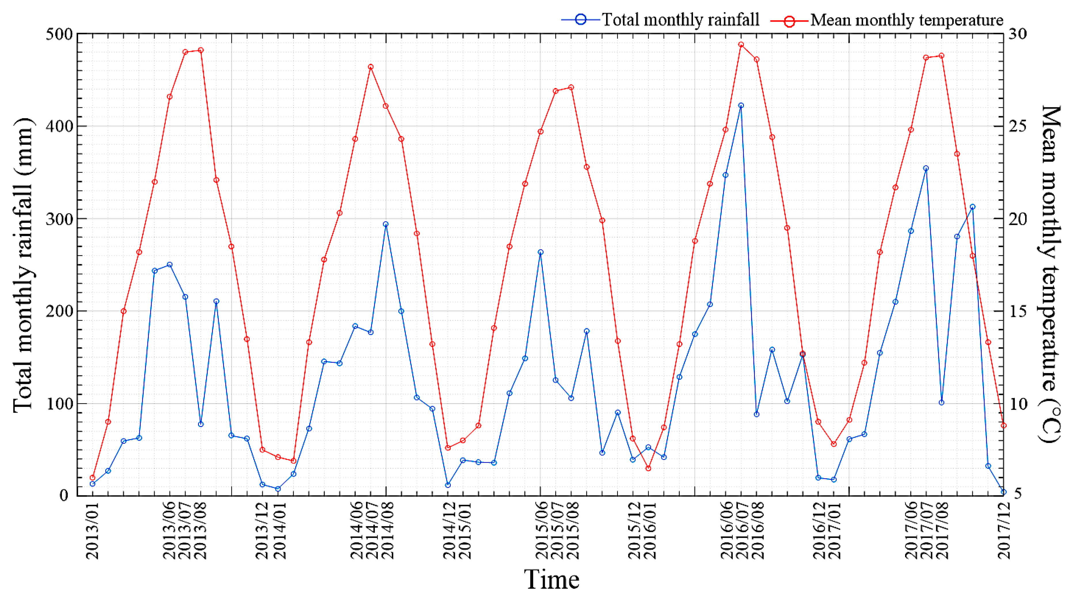
The study area has a subtropical monsoon climate with abundant rainy season rainfall, which is mainly concentrated in summer. According to meteorological and hydrological data of this region, the total monthly precipitation and mean monthly temperature of this region from January 2013 to December 2017 was calculated (Figure 14). The broken line chart of rainfall and temperature indicates that the study area is hot and rainy in summer and cold and dry in winter. And the precipitation in June and July 2016 reached its peak in recent years. Abundant rainfall very readily induces landslides for the following four reasons—(1) heavy rain causes a large amount of surface water to infiltrate into the ground, continuously eroding the weak layer and reducing the mechanical strength of the rock and soil [37]. Additionally, the infiltration pressure of pore water reduces slope stability, thereby inducing landslides [38]; (2) Heavy rain increases underground water and soil water content and significantly decreases the shear strength of soil. Moreover, as the underground water level increases, the soil weight and moisture increases, further resulting in weakening of soil slope convergence, slope displacement and landslides [39,40]; (3) Rainfall leads to an increase of groundwater velocity, which intensifies the subsurface erosion of soil by groundwater, damages slope stability and induces landslides [40]; (4) The continuous increase of groundwater will generate hydrostatic pressure within cracks in the soil mass, increasing the sliding thrust of the slope body and subjecting the sliding surface to upward supporting force, thereby reducing slope stability and inducing landslides [41,42,43].
According to the results of major deformation by month, the increased rainfall in June corresponds to the onset of slow displacement deformation in the study area. Especially after the rainstorm on July 19, the shape variable of the experimental area increased significantly and a new suspected landslide point appeared. With the gradual decrease of rainfall in the subsequent period, no new suspected landslide areas appeared and the existing landslide area was restored naturally; thus, the settlement phenomenon was alleviated to some extent.
5.1.3. Human Factors
With the continued increase of national economic level and improved living standards in recent years—which are linked to the formulation and implementation of the 13th five-year plan—the level of industry and commerce and urban and rural construction is progressively increasing in China. However, the excavation of building foundations, construction of rural roads and the continuous expansion of residential areas have all affected the surrounding natural environment. Landslides caused by human factors can be subdivided into the following four groups. First, slope foot excavation during housing construction leads to degradation and removal of support in the lower part of the slope. Second, due to the influence of geographical location, improper site selection, such as the construction of buildings on slopes, can result in slopes being unable to support significant weight, leading to instability and slides. Third, human effects on water flow (e.g., impounding and drainage) leads to infiltration of water flows into the slope body, increasing the water pressure, softening the soil and rocks and increasing the bulk density of the slope body. Fourth, the continuous extraction of groundwater and the uncontrolled cutting of trees lead to soil erosion on slopes, which changes the original state of the slope and induces landslides.
5.2. A Cross Comparison with PSInSAR Method
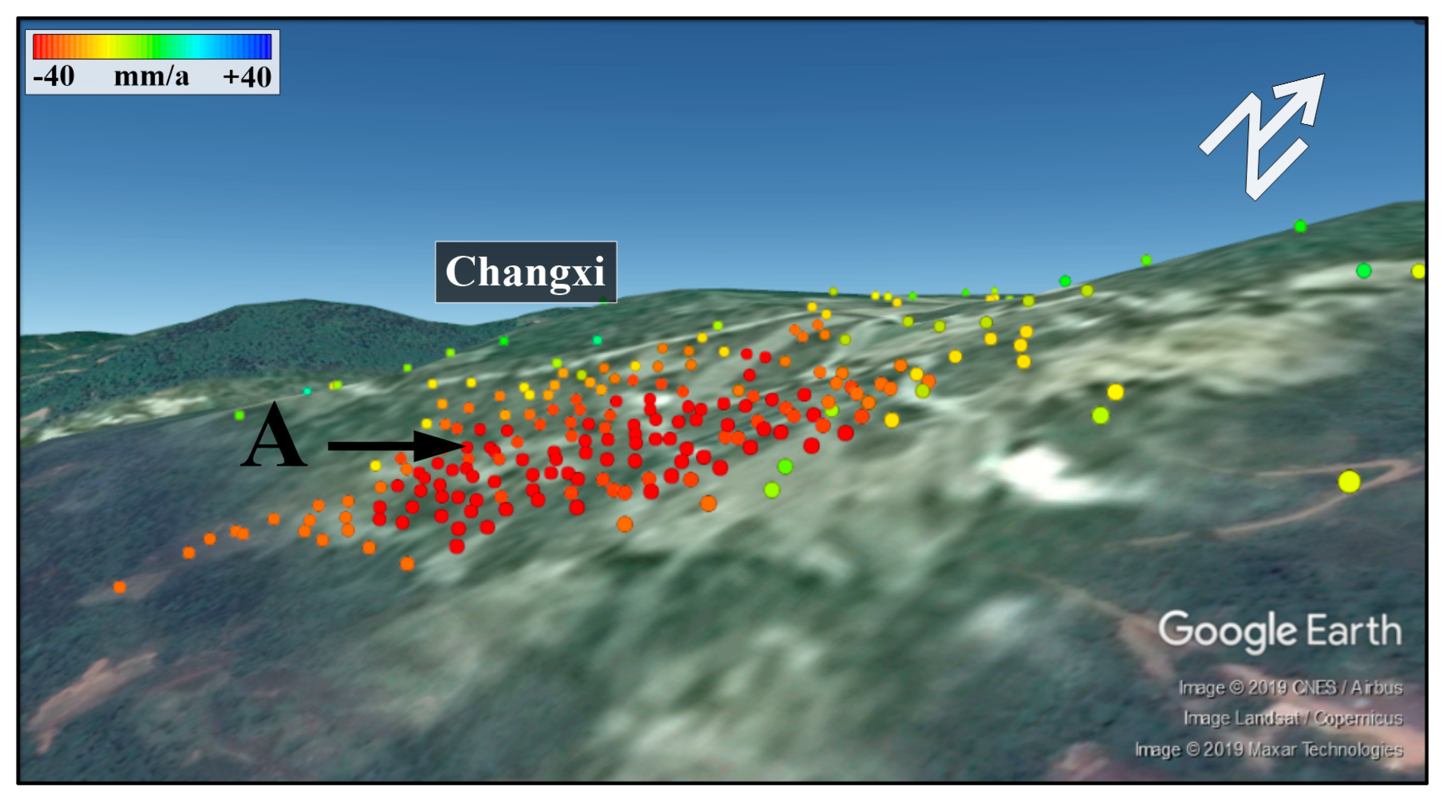
In order to evaluate the reliability of this method, the landslide point A of Qiaotouping in one of the suspected landslide areas was selected for evaluation. This point is both a DS target and a PS target. Firstly, the target deformation time series results obtained by ADS-InSAR and PS-InSAR were compared. Then, the deformation information of the landslide area was compared by combining hydrometeorological and other relevant media reports.
The point A of Qiaotouping Changxi village (see Figure 15) which is PS and also DS, is selected for the evaluation. Because this point is located in the middle of the mountainous region and is on a steep slope strongly affected by rainfall and softening of the rock mass leads to the instability of the slope, which is prone to landslides. The deformation time series results of point A obtained by the ADS-InSAR method are approximately consistent with those obtained by the PS-InSAR method (see Table 2). The RMS value of point A is 1.67 mm, which indicates that the proposed method is robust and reliable.
Other landslide points are located within a landslide group, such as Taoziping (zone 7) (Figure 13). Considering that its geological structure and climatic environment are consistent with the existing landslide areas, there is a high probability of landslides at this suspected landslide point. In addition, some landslide points are affected by other geological disasters and are also classified as suspected landslide areas, such as Jiangjiawan (zone 4) (Figure 13). In July 2016, there was a huge mud-rock flow and flood in this area, which likely led to the current landslide disaster.
6. Conclusions
Although there are currently many mature and reliable methods for landslide monitoring, due to the special climatic environment and complex topographical and geological conditions in mountainous areas, the majority are technically difficult to perform and cannot achieve large-scale and high-density continuous deformation monitoring. In this study, an adaptive distributed scatterer interferometric synthetic aperture radar (ADS-InSAR) method was proposed. Landslide deformation data from Shuibuya district, Hubei province, China was then extracted and analyzed using this method, resulting in the detection of three landslide areas and several suspected landslide points. The calculation results were then compared with those of PS-InSAR.
The results of the proposed ADS-InSAR method are consistent with the calculation trend of the PS-InSAR method, which confirms the reliability of landslide detection by ADS-InSAR. In addition, the proposed method can encrypt the point targets in low coherence regions under the premise of guaranteeing the accuracy of the solution, thereby more effectively inverting local surface deformation and extracting deformation data. The suspected landslide points indicated by the calculation results will be an important reference for various future engineering construction activities. The proposed method can also provide effective early warnings for landslide occurrence and powerful insights for the effective identification and evaluation of landslides in complex and dangerous mountainous areas.
Author Contributions
Conceptualization, H.J.; methodology, H.Z. and L.L.; software, H.Z. and L.L.; validation, H.Z. and L.L.; formal analysis, H.Z. and L.L.; investigation, H.Z. and L.L.; resources, L.L.; data curation, L.L.; writing— H.Z. and L.L.; writing—review and editing, H.J.; visualization, H.Z. and L.L.; supervision, G.L.; project administration, G.L. and H.J.; funding acquisition, H.J.
Funding
This research was funded by the National Key R&D Program of China under Grant 2017YFB0502700, the National Natural Science Foundation of China under Grant 41701535 and Grant 41771402 and the Sichuan Science and Technology Program under Grant 2019YJ0224.
Conflicts of Interest
The authors declare no conflict of interest.
References
- Huang, R. Some catastrophic landslides since the twentieth century in the southwest of China. Landslides 2009, 6, 69–81. [Google Scholar]
- Ding, X.; Montgomery, S.B.; Tsakiri, M.; Swindells, C.F.; Jewell, R.J. Integrated Monitoring Systems for Open Pit Wall Deformation; Meriwa Report No. 186; Australian Centre for Geomechanics: Perth, Australia, 1998. [Google Scholar]
- Thompson, P.W.; Cierlitza, S. Identification of a slope failure over a year before final collapse using multiple monitoring methods. In Geotechnical Instrumentation and Monitoring in Open Pit and Underground Mining; Szwedzicki, T., Ed.; AA Balkema: Rotterdam, The Netherlands, 1993. [Google Scholar]
- Komac, M.; Holley, R.; Mahapatra, P.; van der Marel, H.; Bavec, M. Coupling of GPS/GNSS and radar interferometric data for a 3D surface displacement monitoring of landslides. Landslides 2015, 12, 241–257. [Google Scholar] [CrossRef]
- Huang, Q.; Wang, J.; Deng, J. Slope deformation character analysis based on monitoring results of multiple multi-point borehole extensometer. Chin. J. Rock Mech. Eng. 2009, 28, 2667–2673. [Google Scholar]
- Wu, K.; Yang, X.; Zhou, Y. Application of trigger displacement meter in remote real-time monitoring along mountain highway slope. Subgrade Eng. 2016, 4, 181–185. [Google Scholar]
- Schulz, W.H. Landslide susceptibility revealed by LIDAR imagery and historical records, Seattle, Washington. Eng. Geol. 2007, 89, 67–87. [Google Scholar] [CrossRef]
- Jaboyedoff, M.; Oppikofe, T.; Abellan, A.; Derron, M.; Loye, A.; Metzger, R.; Pedrazzini, A. Use of LIDAR in landslide investigations: A review. Nat. Hazards 2012, 61, 5–28. [Google Scholar] [CrossRef]
- Zhao, C.; Lu, Z.; Zhang, Q.; De La Fuente, J. Large-area landslide detection and monitoring with ALOS/PALSAR imagery data over Northern California and Southern Oregon, USA. Remote Sens. Environ. 2012, 124, 348–359. [Google Scholar] [CrossRef]
- Hu, X.; Wang, T.; Pierson, T.C.; Lu, Z.; Kim, J.-W.; Cecere, T.H. Detecting seasonal landslide movement within the Cascade landslide complex (Washington) using time-series SAR imagery. Remote Sens. Environ. 2016, 187, 49–61. [Google Scholar] [CrossRef] [Green Version]
- Hu, X.; Lu, Z.; Pierson, T.C.; Kramer, R.; George, D.L. Combining InSAR and GPS to Determine Transient Movement and Thickness of a Seasonally Active Low-Gradient Translational Landslide. Geophys. Res. Lett. 2018, 45, 1453–1462. [Google Scholar] [CrossRef]
- Liu, G.; Liu, W.; Huang, D. InSAR Technology and Its Key Problems in Applications. Bull. Surv. Mapp. 2001, 8, 10–12. [Google Scholar]
- Hooper, A. A multi-temporal InSAR method incorporating both persistent scatterer and small baseline approaches. Geophys. Res. Lett. 2008, 35, 302–306. [Google Scholar] [CrossRef]
- Ferretti, A.; Prati, C.; Rocca, F. Permanent scatterers in SAR interferometry. IEEE Trans. Geosci. Remote Sens. 2001, 39, 8–20. [Google Scholar] [CrossRef]
- Berardino, P.; Fornaro, G.; Lanari, R.; Sansosti, E. A new algorithm for surface deformation monitoring based on small baseline differential SAR interferograms. IEEE Trans. Geosci. Remote Sens. 2002, 40, 2375–2383. [Google Scholar] [CrossRef] [Green Version]
- Lei, L.; Zhou, Y.; Li, J.; Burgmann, R. Application of PS-InSAR to monitoring Berkeley landslides. J. Beijing Univ. Aeronaut Astronaut. 2012, 38, 1224–1226. [Google Scholar]
- Zhao, C.; Kang, Y.; Zhang, Q.; Lu, Z.; Li, B. Landslide identification and monitoring along the Jinsha River catchment (Wudongde reservoir area), China, using the InSAR method. Remote Sens. 2018, 10, 993. [Google Scholar] [CrossRef]
- Han, P.; Yang, X.; Bai, L.; Sun, Q. The monitoring and analysis of the coastal lowland subsidence in the southern Hangzhou Bay with an advanced time-series InSAR method. Acta Oceanol. Sin. 2017, 36, 110–118. [Google Scholar] [CrossRef]
- Lee, J.; Pottier, E. Polarimetric Radar Imaging: From Basics to Applications; CRC Press: Boca Raton, FL, USA, 2009. [Google Scholar]
- Jiang, M.; Ding, X.; He, X.; Li, Z.; Shi, G. FaSHPS-InSAR technique for distributed scatterer: A case study over the lost hills oil field, California. Chin. J. Geophys. 2016, 59, 3592–3603. [Google Scholar]
- Jiang, M.; Ding, X.; Hanssen, R.; Malhotra, R.; Chang, L. Fast Statistically Homogeneous Pixel Selection for Covariance Matrix Estimation for Multi-temporal InSAR. IEEE Trans. Geosci. Remote Sens. 2015, 53, 1213–1224. [Google Scholar] [CrossRef]
- Papoulis, A. Probability, Random Variables, and Stochastic Processes; McGraw-Hill Book Company: New York, NY, USA, 1965. [Google Scholar]
- Touzi, R.; Lopes, A.; Bruniquel, J.; Vachon, P.W. Coherence Estimation for SAR Imagery. Coherence Estim. SAR Imag. 1999, 37, 135–149. [Google Scholar]
- Zhao, H.; Chen, W.; Tan, Y. Phase-unwrapping algorithm for the measurement of three-dimensional object shapes. Appl. Opt. 1994, 33, 4497–4500. [Google Scholar] [CrossRef]
- Zebker, H.; Segall, P.; Kampes, B.; Hooper, A. A new method for measuring deformation on volcanoes and other natural terrains using InSAR persistent scatterers. Geophys. Res. Lett. 2004, 31, 31. [Google Scholar]
- Kampes, B. Radar Interferometry: Persistent Scatter Technique. Dordrecht; Springer: Berlin/Heidelberg, Germany, 2006. [Google Scholar]
- Hooper, A.; Zebker, H.A. Phase unwrapping in three dimensions with application to InSAR time series. J. Opt. Soc. Am. A 2007, 24, 2737–2747. [Google Scholar] [CrossRef] [PubMed] [Green Version]
- Dai, K.; Liu, G.; Li, Z.; Li, T.; Yu, B.; Wang, X.; Singleton, A. Extracting Vertical Displacement Rates in Shanghai (China) with Multi-Platform SAR Images. Remote Sens. 2015, 7, 9542–9562. [Google Scholar] [CrossRef] [Green Version]
- Ouchi, K. Recent Trend and Advance of Synthetic Aperture Radar with Selected Topics. Remote Sens. 2013, 5, 716–807. [Google Scholar] [CrossRef] [Green Version]
- Monserrat, O.; Crosetto, M.; Luzi, G. A review of ground-based SAR interferometry for deformation measurement. ISPRS J. Photogramm. Remote Sens. 2014, 93, 40–48. [Google Scholar] [CrossRef] [Green Version]
- Samiei-Esfahany, S.; Martins, J.E.; Van Leijen, F.; Hanssen, R.F. Phase Estimation for Distributed Scatterers in InSAR Stacks Using Integer Least Squares Estimation. IEEE Trans. Geosci. Remote Sens. 2016, 54, 1–17. [Google Scholar] [CrossRef]
- Fan, Y.; Li, Q.; Chen, Z. Microscope Study on Softening Characteristics of Shale in Shuibuya Project. J. Yangtze River Sci. Res. Inst. 1998, 15, 48–50. [Google Scholar]
- Huang, B. Prevention and Consideration of Geological Disasters in Reservoir Area of Shuibuya Hydroproject. Resour. Environ. Eng. 2009, 23, 123–125. [Google Scholar]
- Yang, Y.; Chen, J.; Yang, J. Stability analysis and countermeasures of landslide in Changyang Luanshijiao. Resour. Environ. Eng. 2012, 26, 52–54. [Google Scholar]
- Liu, P.; Li, Z.; Hoey, T.; Kincal, C.; Zhang, J.; Zeng, Q.; Muller, J.-P. Using advanced InSAR time series techniques to monitor landslide movements in Badong of the Three Gorges region, China. Int. J. Appl. Earth Obs. Geoinf. 2013, 21, 253–264. [Google Scholar] [CrossRef]
- Peng, K.; Li, Q.; Zhao, X.; Li, Y.; He, J. Quantitative evaluation of geological disaster liability based on RS and GIS analysis: A case study of Wufeng County, Hubei Province. Earth Sci. Front. 2012, 19, 221–229. [Google Scholar]
- Kang, Y.; Zhao, C.; Zhang, Q.; Lu, Z.; Li, B. Application of InSAR Techniques to an Analysis of the Guanling Landslide. Remote Sens. 2017, 9, 1046. [Google Scholar] [CrossRef]
- Klubertanz, G.; Laloui, L.; Vulliet, L. Identification of mechanisms for landslide type initiation of debris flows. Eng. Geol. 2009, 109, 114–123. [Google Scholar] [CrossRef]
- Sun, Q.; Zhang, L.; Ding, X.; Hu, J.; Li, Z.-W.; Zhu, J.; Ding, X. Slope deformation prior to Zhouqu, China landslide from InSAR time series analysis. Remote Sens. Environ. 2015, 156, 45–57. [Google Scholar] [CrossRef]
- Huang, R. Mechanisms of large-scale landslides in China. Bull. Eng. Geol. Environ. 2012, 71, 161–170. [Google Scholar] [CrossRef]
- Wu, H.; Feng, M.; Jiao, Y.; Li, H. Analysis of sliding mechanism of accumulation horizon landslide under rainfall condition. Rock Soil Mech. 2010, 31, 0324–0329. [Google Scholar]
- Fustos, I.; Remy, D.; Abarca-Del-Rio, R.; Munoz, A. Slow movements observed with in situ and remote-sensing techniques in the central zone of Chile. Int. J. Remote Sens. 2017, 38, 7514–7530. [Google Scholar] [CrossRef]
- Kiseleva, E.; Mikhailov, V.; Smolyaninova, E.; Dmitriev, P.; Golubev, V.; Timoshkina, E.; Hooper, A.; Samiei-Esfahany, S.; Hanssen, R. PS-InSAR Monitoring of Landslide Activity in the Black Sea Coast of the Caucasus. Procedia Technol. 2014, 16, 404–413. [Google Scholar] [Green Version]
Figure 1.
Coherence coefficient diagram for Yunnan province, southwest China.

Figure 2.
Block coherence coefficient diagram for Yunnan province, southwest China; (a) 8 × 8 blocks partition; (b) 16 × 16 blocks partition; (c) 32 × 32 blocks partition; (d) 64 × 64 blocks partition;.
Figure 2.
Block coherence coefficient diagram for Yunnan province, southwest China; (a) 8 × 8 blocks partition; (b) 16 × 16 blocks partition; (c) 32 × 32 blocks partition; (d) 64 × 64 blocks partition;.


Figure 3.
Relationship between block threshold and extracted points.

Figure 4.
Map of the study area in Hubei province, China.

Figure 5.
Image of the average amplitude in the study area.

Figure 6.
Spatial and temporal baseline profiles of interference.

Figure 7.
(a) Differential interference result and (b) differential interference result superimposed on the amplitude image.
Figure 7.
(a) Differential interference result and (b) differential interference result superimposed on the amplitude image.

Figure 8.
(a) Coherence coefficient diagram and (b) block result diagram.

Figure 9.
Selected distributed scatterer (DS) distribution for (a) the adaptive threshold and (b) the empirical coherence threshold.
Figure 9.
Selected distributed scatterer (DS) distribution for (a) the adaptive threshold and (b) the empirical coherence threshold.

Figure 10.
Comparison of DS distribution in the Luanshijiao area for (a) the DS result selected by the adaptive threshold and (b) the DS result selected by the empirical threshold.
Figure 10.
Comparison of DS distribution in the Luanshijiao area for (a) the DS result selected by the adaptive threshold and (b) the DS result selected by the empirical threshold.

Figure 11.
Annual average deformation rate map.

Figure 12.
Major deformation results per month.

Figure 13.
Landslide detection results showing the distribution of seven landslide areas (white areas show confirmed landslide areas and red areas show suspected landslide areas).
Figure 13.
Landslide detection results showing the distribution of seven landslide areas (white areas show confirmed landslide areas and red areas show suspected landslide areas).

Figure 14.
Total monthly rainfall volumes and mean monthly temperature in the study area.

Figure 15.
Annual average settlement rate of landslide monitoring point A.


Table 1.
Comparison of extraction results.
| Block Threshold | DS Points (pieces) | Computational Time (s) |
|---|---|---|
| Global threshold | 113,423 | 1.23 |
| 4 × 4 | 124,645 | 2.08 |
| 8 × 8 | 132,261 | 3.86 |
| 16 × 16 | 139,107 | 4.71 |
| 32 × 32 | 141,211 | 5.63 |
| 64 × 64 | 142,256 | 7.32 |
Table 2.
The deformation time series results of point A obtained by adaptive distributed scatterer interferometric synthetic aperture radar (ADS-InSAR) and persistent scatterer interferometric synthetic aperture radar (PS-InSAR).
Table 2.
The deformation time series results of point A obtained by adaptive distributed scatterer interferometric synthetic aperture radar (ADS-InSAR) and persistent scatterer interferometric synthetic aperture radar (PS-InSAR).
| 2016/03/05 | 2016/04/22 | 2016/05/16 | 2016/06/09 | 2016/07/03 | 2016/08/20 | |
| ADS (mm) | 1.453 | −2.191 | −1.346 | −12.336 | −22.503 | −9.701 |
| PS (mm) | 2.392 | −2.739 | −1.932 | −15.795 | −23.627 | −11.325 |
| 2016/09/25 | 2016/10/07 | 2016/10/31 | 2016/11/12 | 2016/12/30 | 2017/01/11 | |
| ADS (mm) | −12.471 | 0.164 | 0.110 | −0.951 | 0.000 | −3.713 |
| PS (mm) | −13.543 | −1.325 | 0.369 | −1.189 | 0.000 | −4.892 |
| 2017/01/23 | 2017/02/16 | 2017/02/28 | 2017/03/12 | 2017/03/24 | 2017/04/05 | |
| ADS( mm) | 1.141 | −1.243 | 0.174 | 0.928 | 0.096 | −0.390 |
| PS (mm) | 1.426 | −1.554 | 0.218 | 1.160 | 0.215 | −3.150 |
© 2019 by the authors. Licensee MDPI, Basel, Switzerland. This article is an open access article distributed under the terms and conditions of the Creative Commons Attribution (CC BY) license (http://creativecommons.org/licenses/by/4.0/).
Share and Cite
MDPI and ACS Style
Jia, H.; Zhang, H.; Liu, L.; Liu, G. Landslide Deformation Monitoring by Adaptive Distributed Scatterer Interferometric Synthetic Aperture Radar. Remote Sens. 2019, 11, 2273. https://0-doi-org.brum.beds.ac.uk/10.3390/rs11192273
AMA Style
Jia H, Zhang H, Liu L, Liu G. Landslide Deformation Monitoring by Adaptive Distributed Scatterer Interferometric Synthetic Aperture Radar. Remote Sensing. 2019; 11(19):2273. https://0-doi-org.brum.beds.ac.uk/10.3390/rs11192273
Chicago/Turabian StyleJia, Hongguo, Hao Zhang, Luyao Liu, and Guoxiang Liu. 2019. "Landslide Deformation Monitoring by Adaptive Distributed Scatterer Interferometric Synthetic Aperture Radar" Remote Sensing 11, no. 19: 2273. https://0-doi-org.brum.beds.ac.uk/10.3390/rs11192273
Note that from the first issue of 2016, this journal uses article numbers instead of page numbers. See further details here.