Figure 1.
Illustration of a residual block.
Figure 1.
Illustration of a residual block.
Figure 2.
The structure of convolutional LSTM (CLSTM). Left, zoomed view of the inner computational unit called the memory cell. “” and “ ” represent the matrix addition and the dot product, respectively.
Figure 2.
The structure of convolutional LSTM (CLSTM). Left, zoomed view of the inner computational unit called the memory cell. “” and “ ” represent the matrix addition and the dot product, respectively.
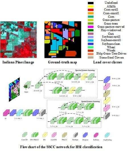
Figure 3.
Flowchart of the SSCC network for HSI classification.
Figure 3.
Flowchart of the SSCC network for HSI classification.
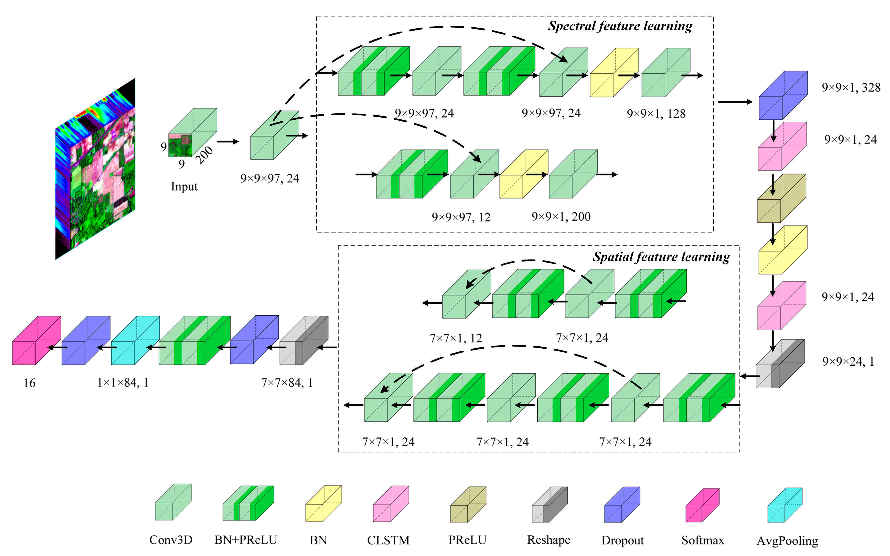
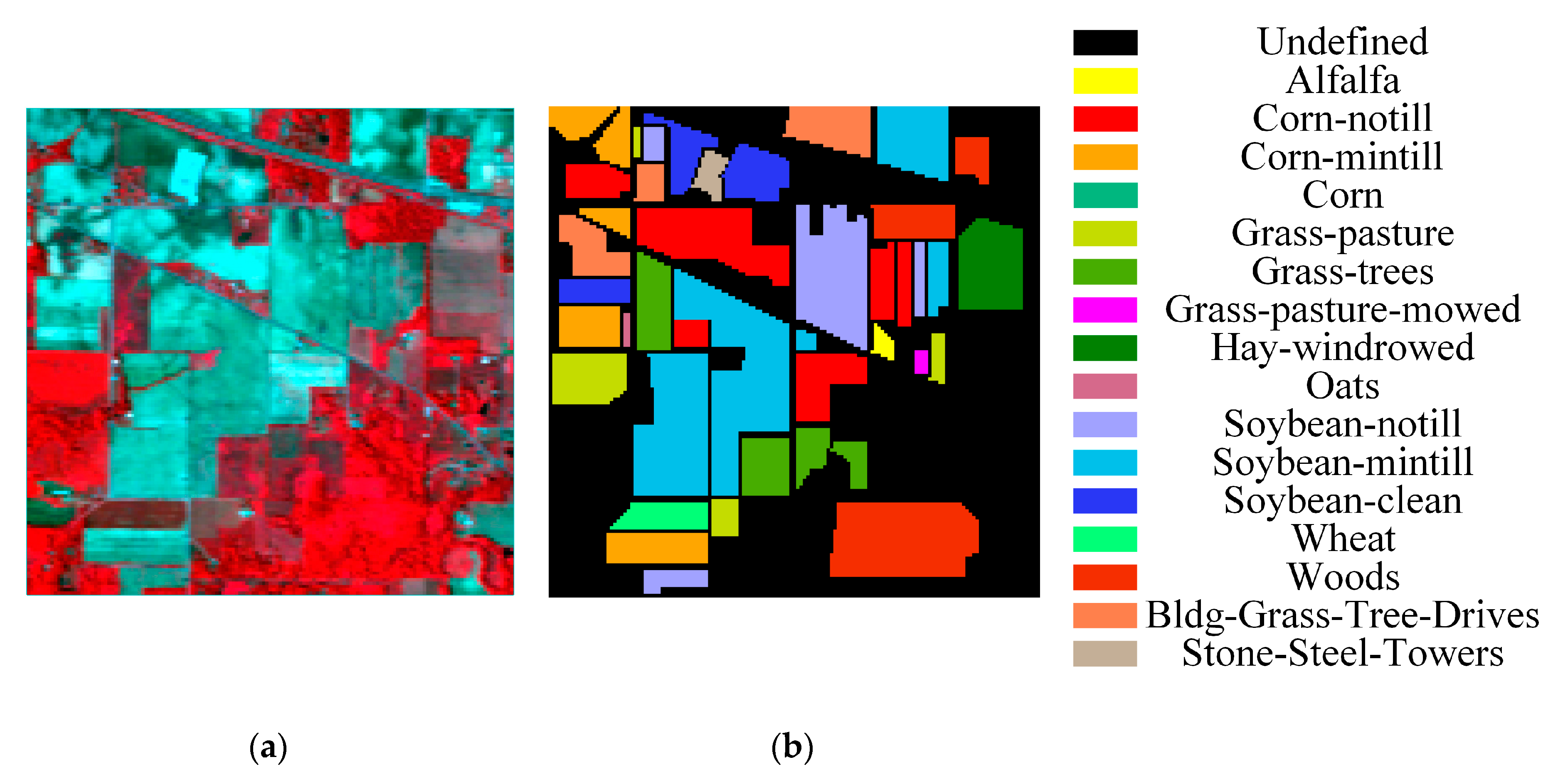
Figure 4.
Indiana Pines dataset: (a) false-color composite of Indiana Pines, (b) ground-truth map.
Figure 4.
Indiana Pines dataset: (a) false-color composite of Indiana Pines, (b) ground-truth map.
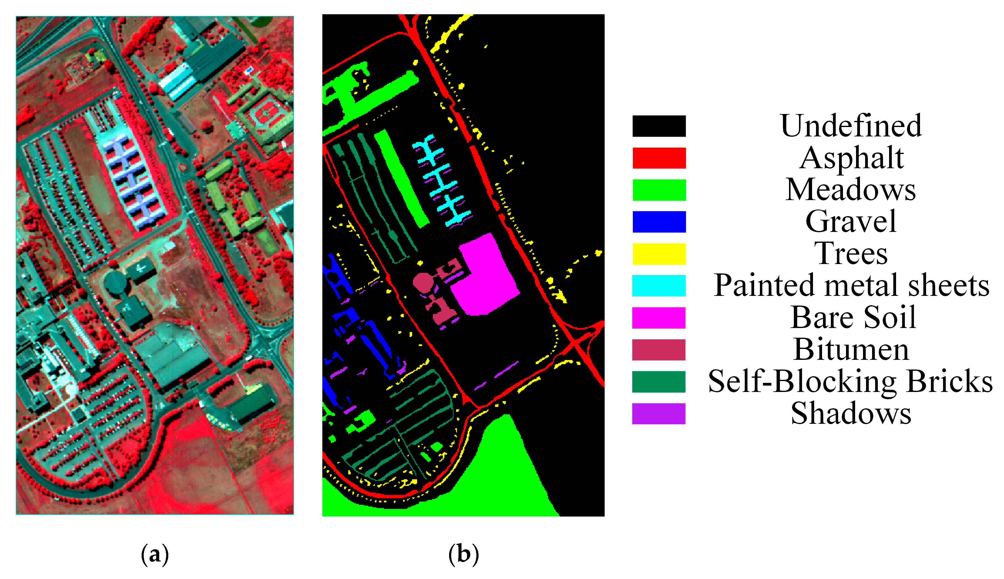
Figure 5.
University of Pavia dataset: (a) false-color composite of the University of Pavia, (b) ground-truth map.
Figure 5.
University of Pavia dataset: (a) false-color composite of the University of Pavia, (b) ground-truth map.
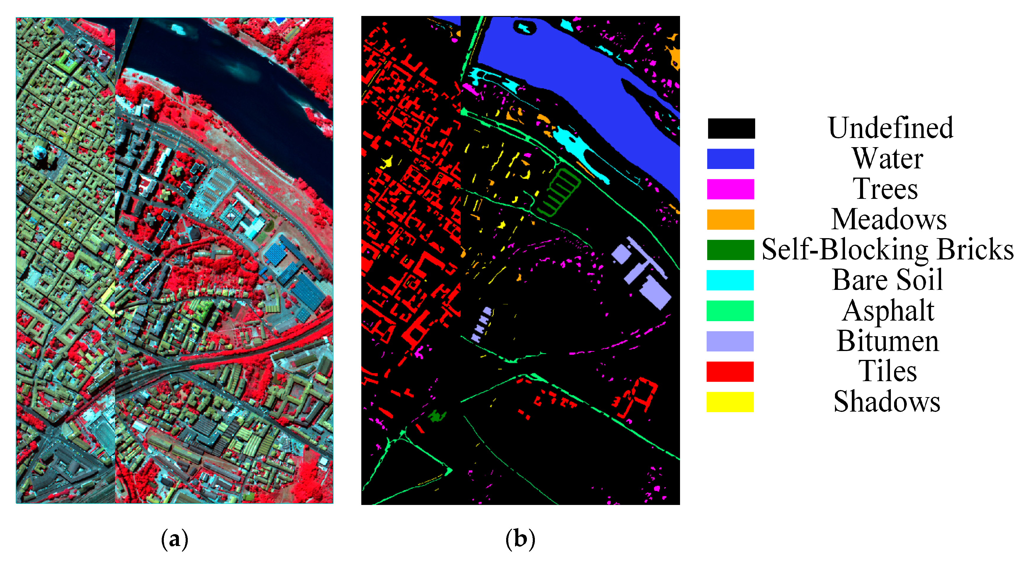
Figure 6.
Pavia Center dataset: (a) false-color composite of Pavia Center, (b) ground-truth map.
Figure 6.
Pavia Center dataset: (a) false-color composite of Pavia Center, (b) ground-truth map.
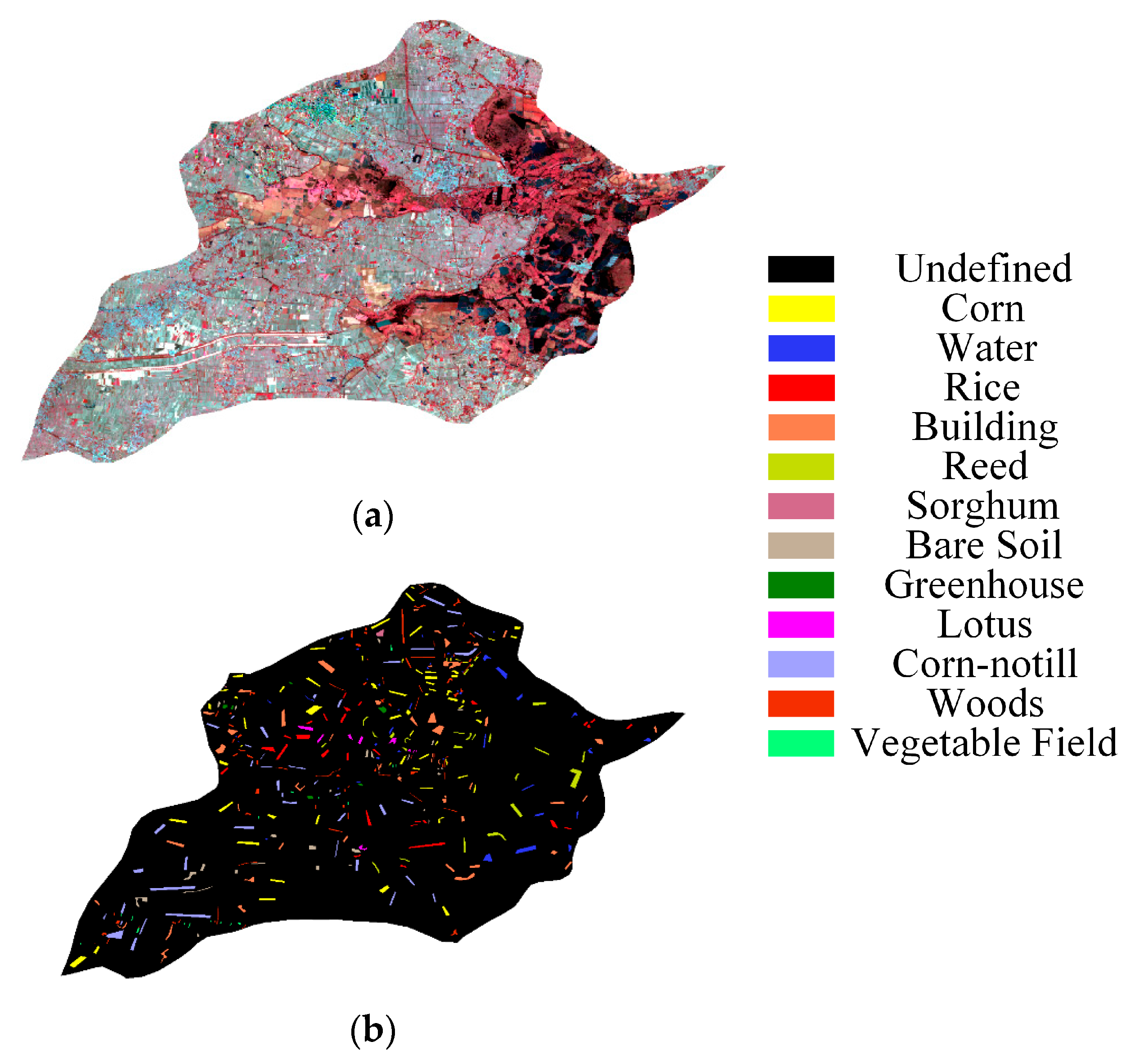
Figure 7.
GF-5 dataset of Anxin County, Xiongan New Area: (a) false-color composite of GF-5, (b) ground-truth map.
Figure 7.
GF-5 dataset of Anxin County, Xiongan New Area: (a) false-color composite of GF-5, (b) ground-truth map.
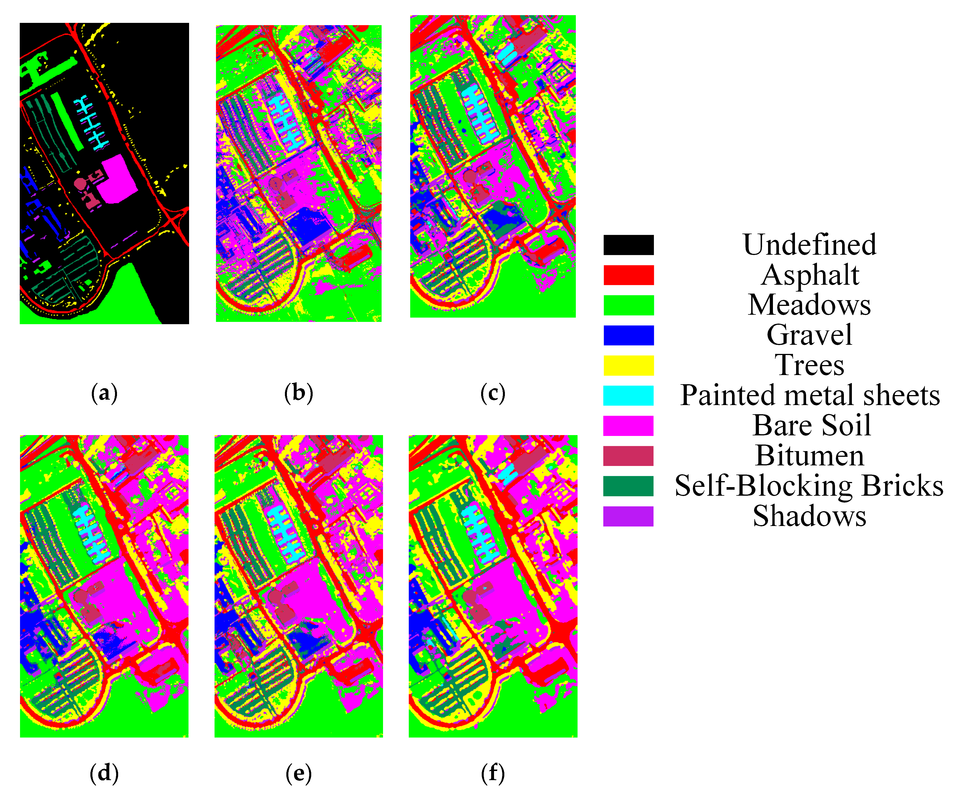
Figure 8.
Classification maps for Indiana Pines dataset: (a) Ground-truth map, (b) SSLSTMs, OA = 67.30%, (c) 3D CNN, OA = 79.22%, (d) FDSSC, OA = 92.77%, (e) SSRN, OA = 95.21%, (f) SSCC, OA = 97.70%.
Figure 8.
Classification maps for Indiana Pines dataset: (a) Ground-truth map, (b) SSLSTMs, OA = 67.30%, (c) 3D CNN, OA = 79.22%, (d) FDSSC, OA = 92.77%, (e) SSRN, OA = 95.21%, (f) SSCC, OA = 97.70%.
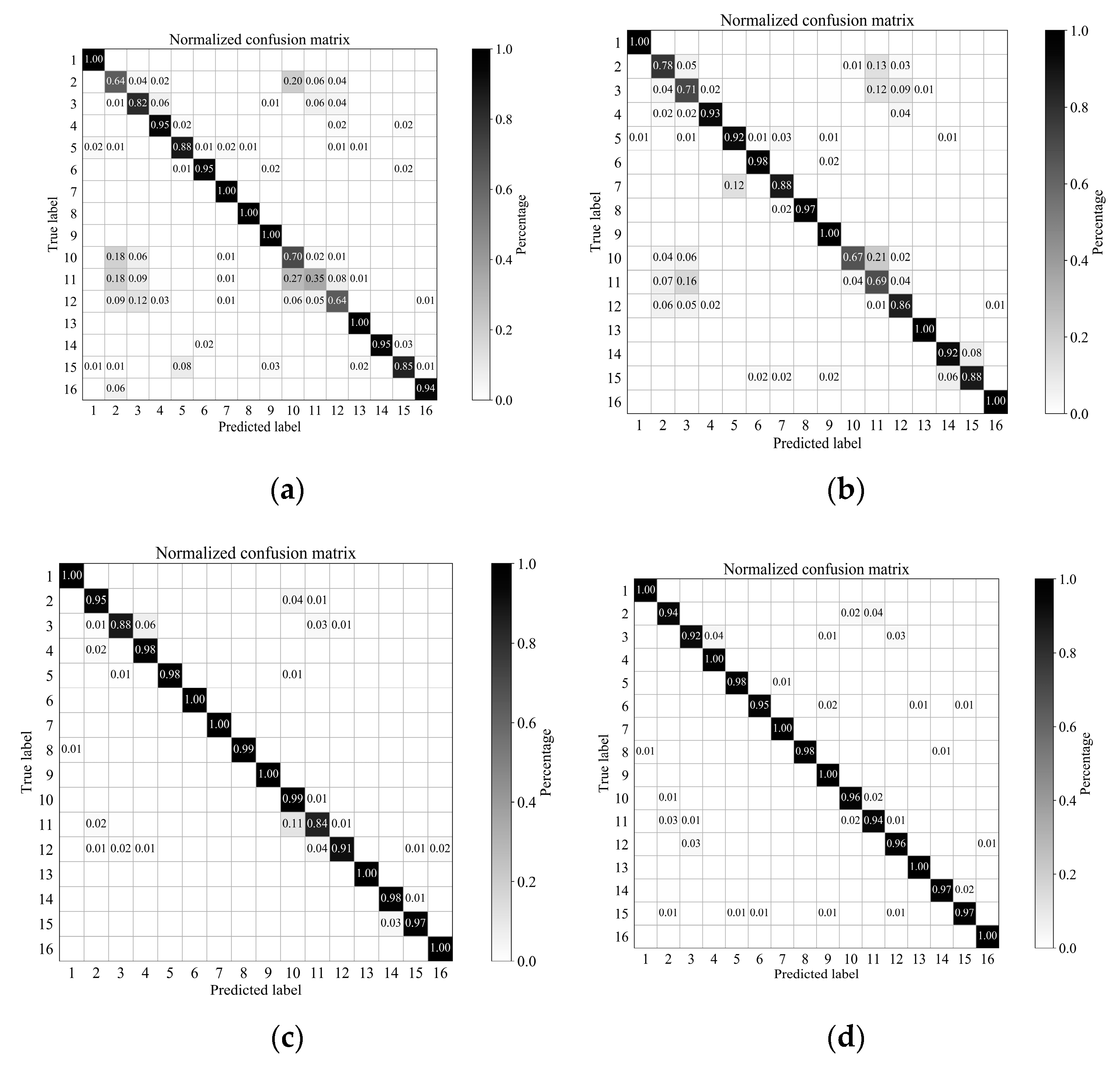
Figure 9.
Indiana Pines dataset: Normalized confusion matrix of classification results using different methods (displaying value greater than 0.005): (a) SSLSTMs, (b) 3D CNN, (c) FDSSC, (d) SSRN, (e) SSCC.
Figure 9.
Indiana Pines dataset: Normalized confusion matrix of classification results using different methods (displaying value greater than 0.005): (a) SSLSTMs, (b) 3D CNN, (c) FDSSC, (d) SSRN, (e) SSCC.
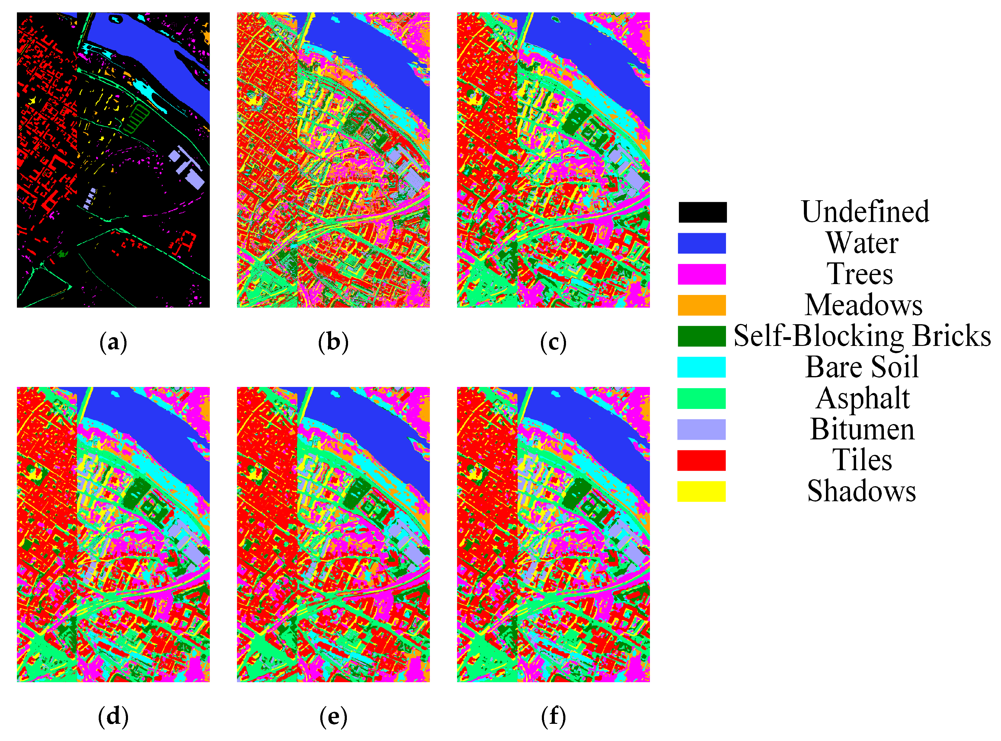
Figure 10.
Classification maps for University of Pavia dataset: (a) Ground-truth map, (b) SSLSTMs, OA = 83.36%, (c) 3D CNN, OA = 91.71%, (d) FDSSC, OA = 98.39%, (e) SSRN, OA = 99.12%, (f) SSCC, OA = 99.71%.
Figure 10.
Classification maps for University of Pavia dataset: (a) Ground-truth map, (b) SSLSTMs, OA = 83.36%, (c) 3D CNN, OA = 91.71%, (d) FDSSC, OA = 98.39%, (e) SSRN, OA = 99.12%, (f) SSCC, OA = 99.71%.
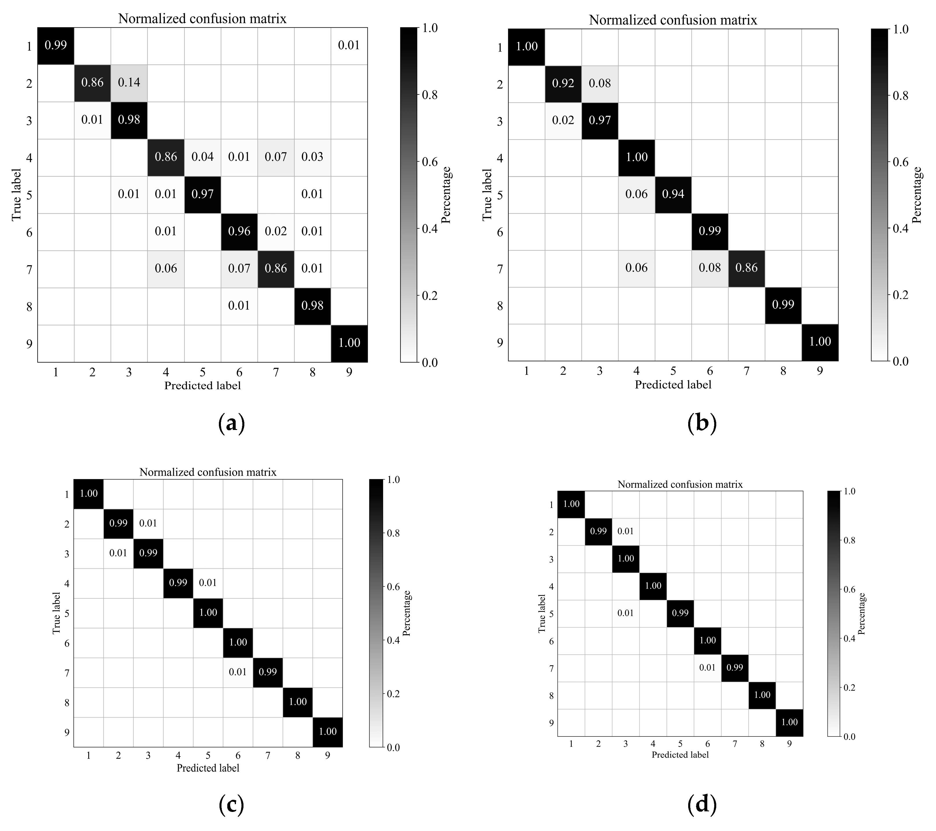
Figure 11.
University of Pavia dataset: Normalized confusion matrix of classification results using different methods (displaying value greater than 0.005): (a) SSLSTMs, (b) 3D CNN, (c) FDSSC, (d) SSRN, (e) SSCC.
Figure 11.
University of Pavia dataset: Normalized confusion matrix of classification results using different methods (displaying value greater than 0.005): (a) SSLSTMs, (b) 3D CNN, (c) FDSSC, (d) SSRN, (e) SSCC.
Figure 12.
Classification maps for Pavia Center dataset: (a) Ground-truth map, (b) SSLSTMs, OA = 97.16%, (c) 3D CNN, OA = 98.33%, (d) FDSSC, OA = 99.83%, (e) SSRN, OA = 99.76%, (f) SSCC, OA = 99.84%.
Figure 12.
Classification maps for Pavia Center dataset: (a) Ground-truth map, (b) SSLSTMs, OA = 97.16%, (c) 3D CNN, OA = 98.33%, (d) FDSSC, OA = 99.83%, (e) SSRN, OA = 99.76%, (f) SSCC, OA = 99.84%.
Figure 13.
University of Pavia: Normalized confusion matrix of classification results using different methods (displaying value greater than 0.005): (a) SSLSTMs, (b) 3D CNN, (c) FDSSC, (d) SSRN, (e) SSCC.
Figure 13.
University of Pavia: Normalized confusion matrix of classification results using different methods (displaying value greater than 0.005): (a) SSLSTMs, (b) 3D CNN, (c) FDSSC, (d) SSRN, (e) SSCC.
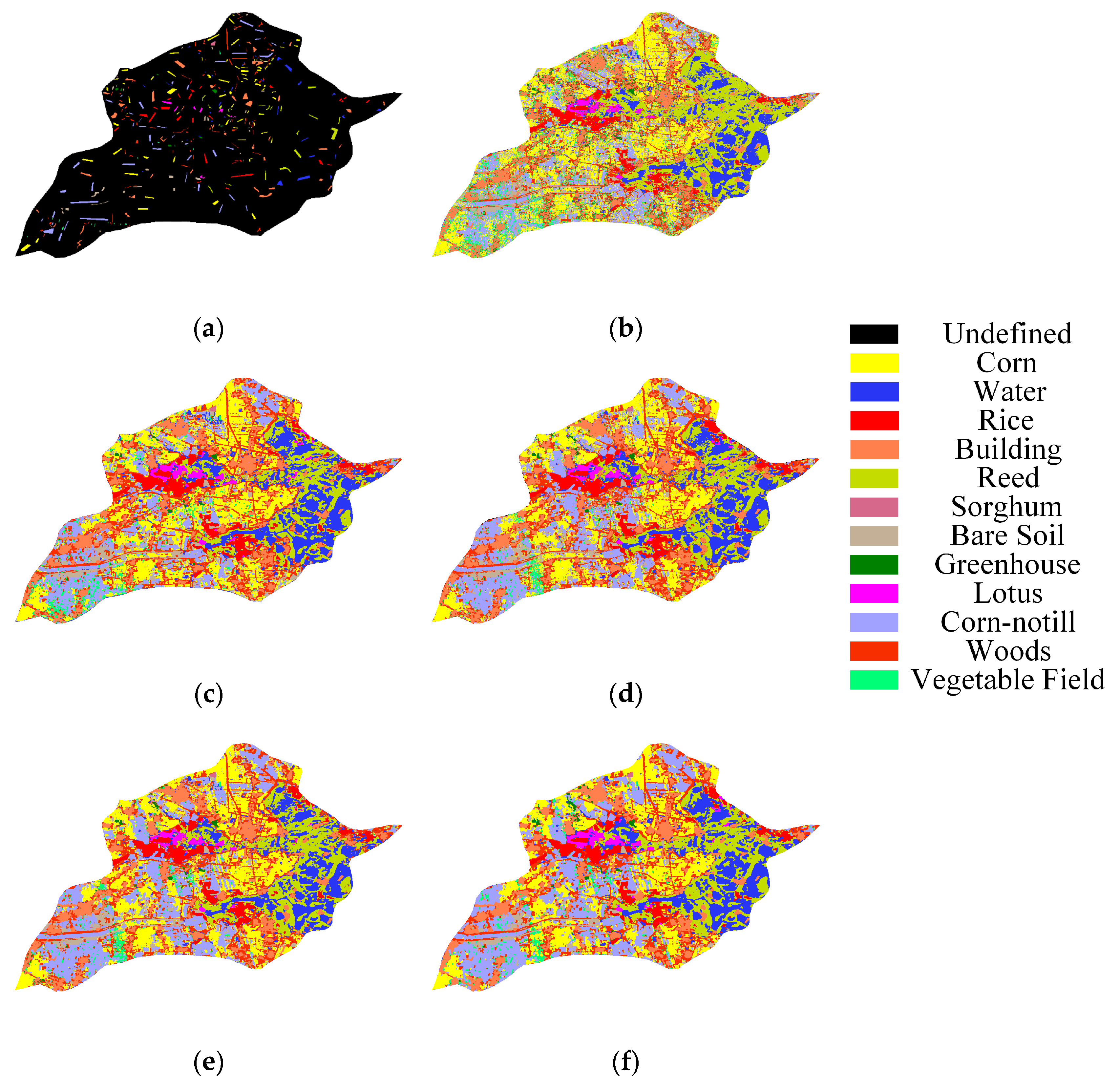
Figure 14.
Classification maps for GF5AX dataset: (a) Ground-truth map, (b) SSLSTMs, OA = 87.47%, (c) 3D CNN, OA = 96.75%, (d) FDSSC, OA = 98.46%, (e) SSRN, OA = 99.32%, (f) SSCC, OA = 99.37%.
Figure 14.
Classification maps for GF5AX dataset: (a) Ground-truth map, (b) SSLSTMs, OA = 87.47%, (c) 3D CNN, OA = 96.75%, (d) FDSSC, OA = 98.46%, (e) SSRN, OA = 99.32%, (f) SSCC, OA = 99.37%.
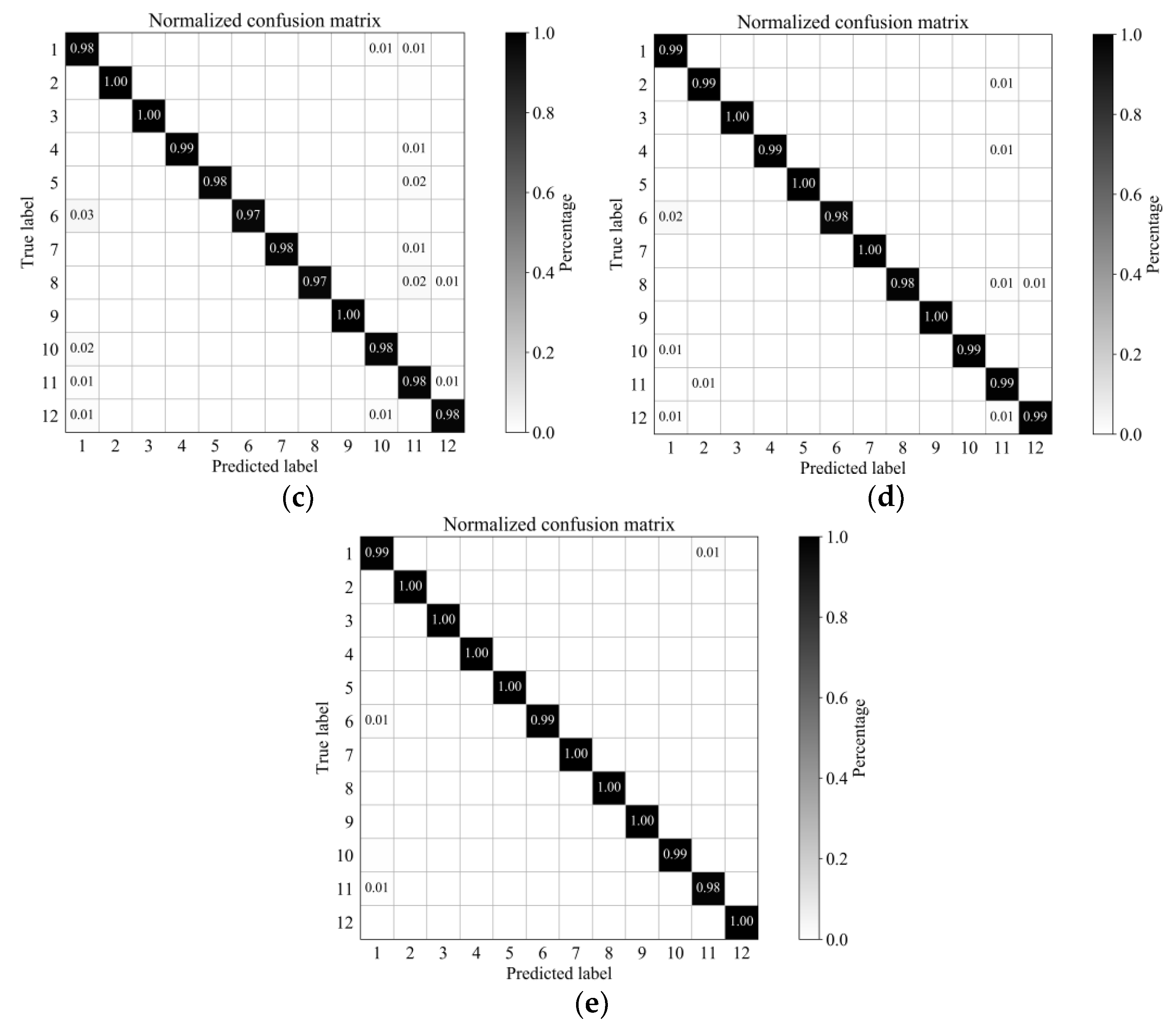
Figure 15.
GF5AX dataset: Normalized confusion matrix of classification results using different methods (displaying value greater than 0.005): (a) SSLSTMs, (b) 3D CNN, (c) FDSSC, (d) SSRN, (e) SSCC.
Figure 15.
GF5AX dataset: Normalized confusion matrix of classification results using different methods (displaying value greater than 0.005): (a) SSLSTMs, (b) 3D CNN, (c) FDSSC, (d) SSRN, (e) SSCC.
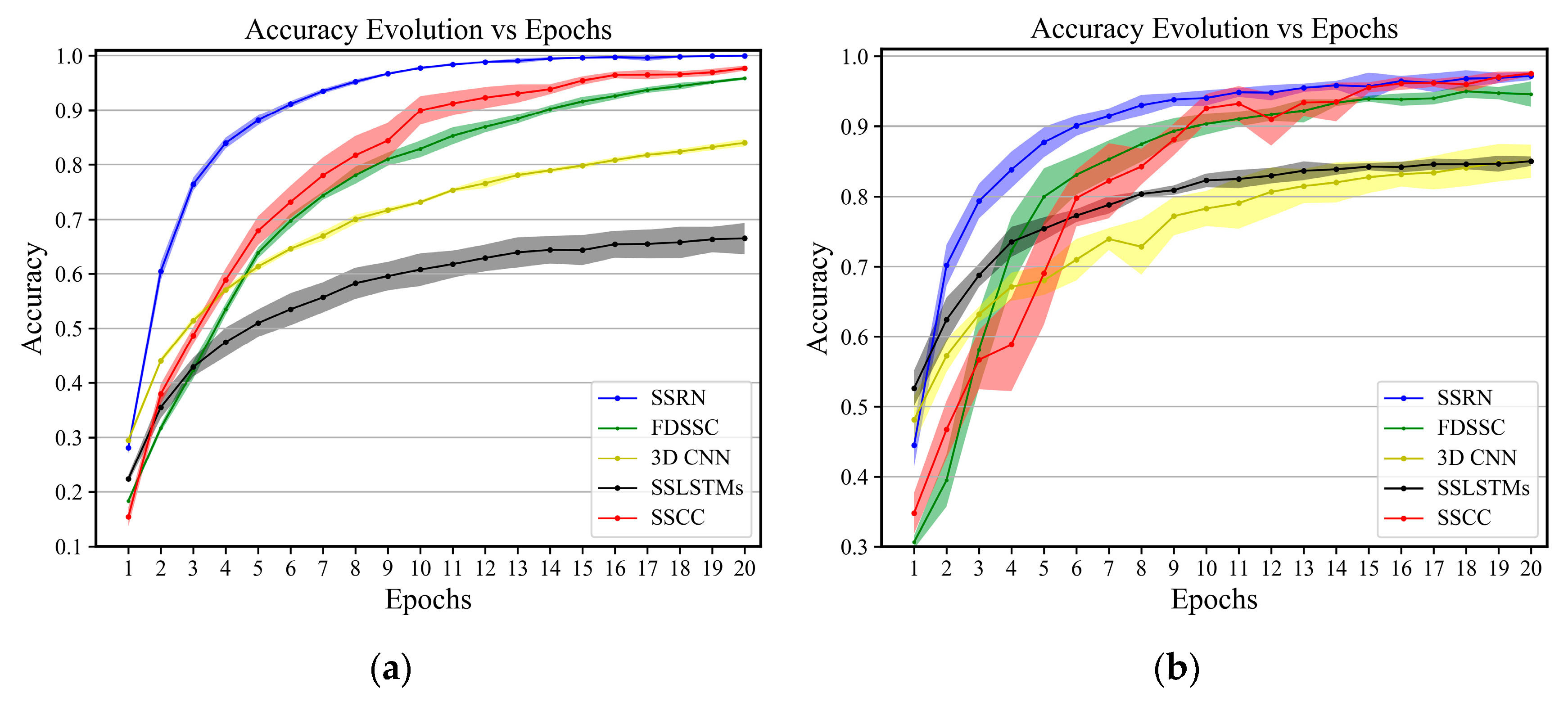
Figure 16.
Indiana Pines: Evolution of the accuracy in terms of epochs on (a) training data and (b) validation data. The shadow shows the standard deviation of the accuracy for five executions.
Figure 16.
Indiana Pines: Evolution of the accuracy in terms of epochs on (a) training data and (b) validation data. The shadow shows the standard deviation of the accuracy for five executions.
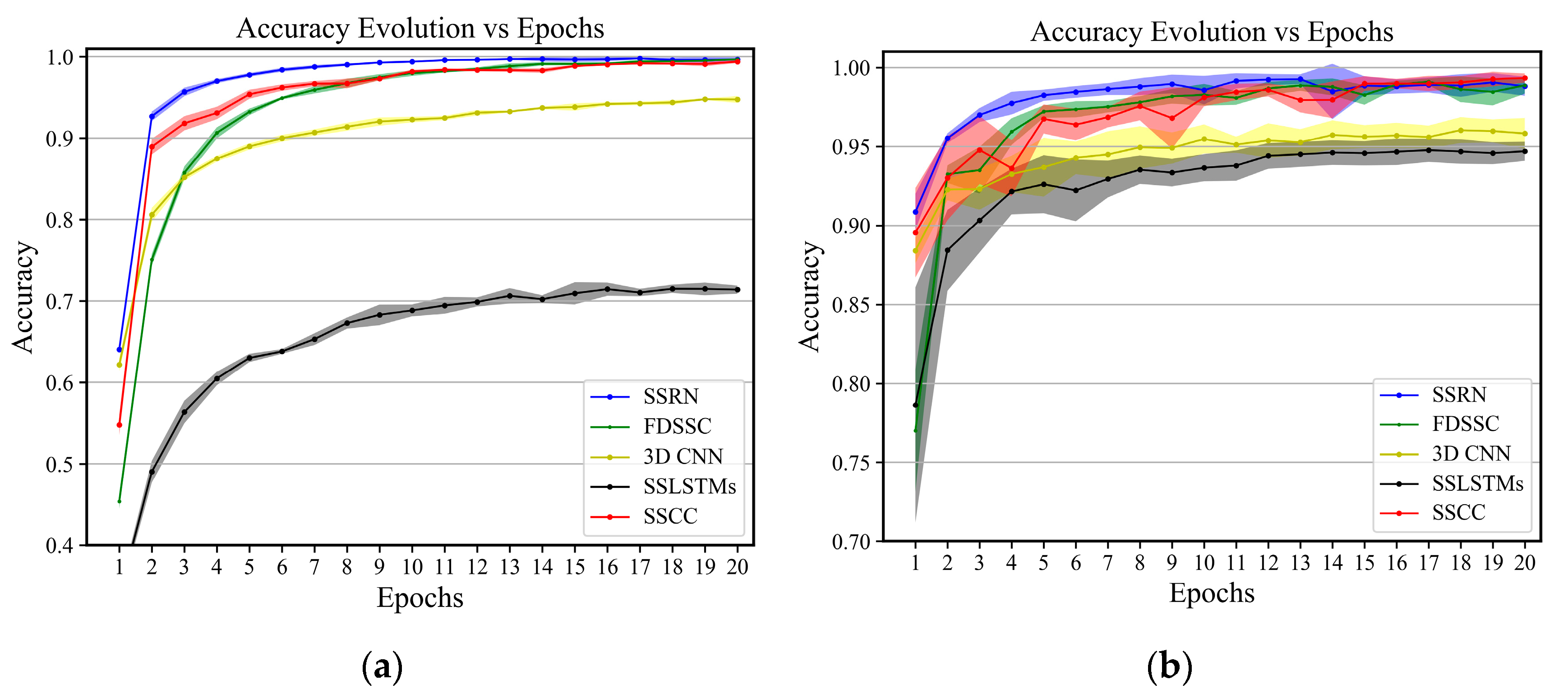
Figure 17.
University of Pavia: Evolution of the accuracy in terms of epochs on (a) training data and (b) validation data. The shadow shows the standard deviation of the accuracy for five executions.
Figure 17.
University of Pavia: Evolution of the accuracy in terms of epochs on (a) training data and (b) validation data. The shadow shows the standard deviation of the accuracy for five executions.
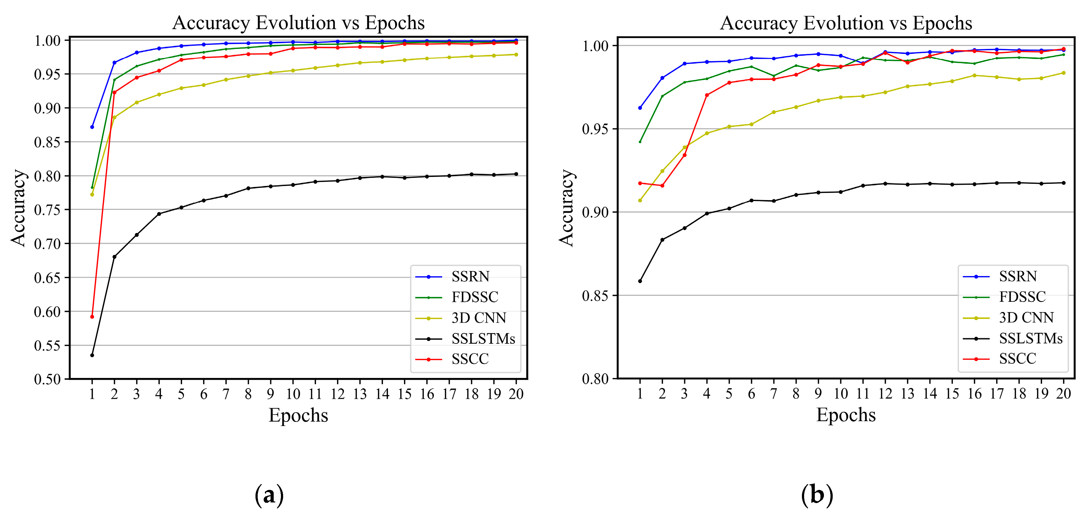
Figure 18.
Pavia Center: Evolution of the accuracy in terms of epochs on (a) training data and (b) validation data. The shadow shows the standard deviation of the accuracy for five executions.
Figure 18.
Pavia Center: Evolution of the accuracy in terms of epochs on (a) training data and (b) validation data. The shadow shows the standard deviation of the accuracy for five executions.
Figure 19.
GF-5 datasets of Anxin County: Evolution of the accuracy in terms of epochs on (a) training data and (b) validation data.
Figure 19.
GF-5 datasets of Anxin County: Evolution of the accuracy in terms of epochs on (a) training data and (b) validation data.
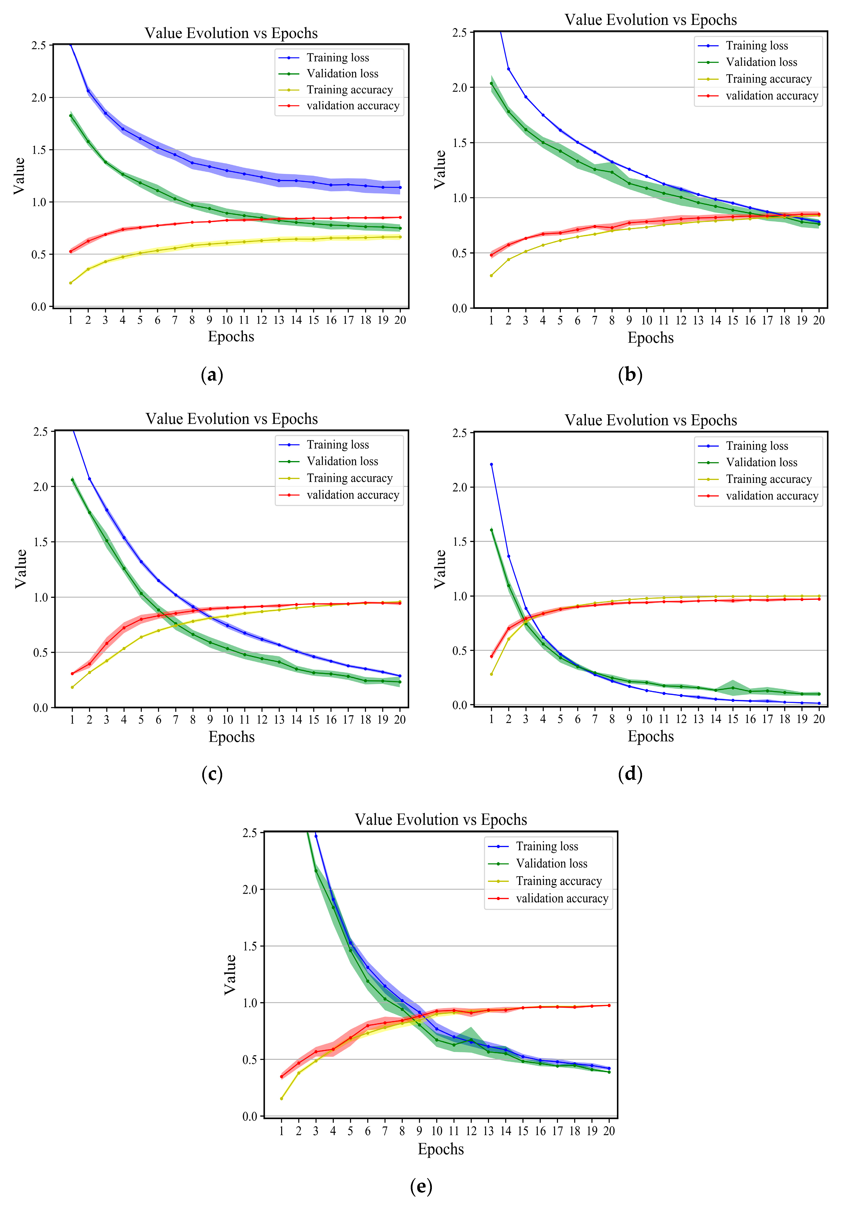
Figure 20.
Indiana Pines dataset: Evolution of the accuracy or loss in terms of epochs on training and validation data. The shadow shows the standard deviation of the values for five executions: (a) SSLSTMs, (b) 3D CNN, (c) FDSSC, (d) SSRN, (e) SSCC.
Figure 20.
Indiana Pines dataset: Evolution of the accuracy or loss in terms of epochs on training and validation data. The shadow shows the standard deviation of the values for five executions: (a) SSLSTMs, (b) 3D CNN, (c) FDSSC, (d) SSRN, (e) SSCC.
Figure 21.
GF5AX dataset: Evolution of the accuracy or loss in terms of epochs on training and validation data. (a) SSLSTMs, (b) 3D CNN, (c) FDSSC, (d) SSRN, (e) SSCC.
Figure 21.
GF5AX dataset: Evolution of the accuracy or loss in terms of epochs on training and validation data. (a) SSLSTMs, (b) 3D CNN, (c) FDSSC, (d) SSRN, (e) SSCC.
Table 1.
Number of training samples used in the Indiana Pines dataset.
Table 1.
Number of training samples used in the Indiana Pines dataset.
| NO. | Indiana Pines (IP) | GF-5 Dataset (GF5AX) |
| Class | Train | Total | Class | Train | Total |
| 1 | Alfalfa | 33 | 46 | Corn | 1630 | 5434 |
| 2 | Corn-notill | 200 | 1428 | Water-body | 627 | 2089 |
| 3 | Corn-mintill | 200 | 830 | Rice | 713 | 2377 |
| 4 | Corn | 181 | 237 | Building | 1571 | 5237 |
| 5 | Grass-pasture | 200 | 483 | Reed | 707 | 2356 |
| 6 | Grass-trees | 200 | 730 | Sorghum | 53 | 177 |
| 7 | Grass-pasture-mowed | 20 | 28 | Bare-land | 475 | 1583 |
| 8 | Hay-windrowed | 200 | 478 | Greenhouse | 122 | 408 |
| 9 | Oats | 14 | 20 | Lotus | 194 | 648 |
| 10 | Soybean-notill | 200 | 972 | Corn-notill | 1632 | 5440 |
| 11 | Soybean-mintill | 200 | 2455 | Woods | 853 | 2844 |
| 12 | Soybean-clean | 200 | 593 | Vegetable-field | 69 | 231 |
| 13 | Wheat | 143 | 205 | | | |
| 14 | Woods | 200 | 1265 | | | |
| 15 | Bldg-Grass-Tree-Drives | 200 | 386 | | | |
| 16 | Stone-Steel-Towers | 75 | 93 | | | |
| | Total | 2466 | 10,249 | Total | 8646 | 28,824 |
| NO. | University of Pavia (UP) | Pavia Center (PC) |
| Class | Train. | Total | Class | Train. | Total |
| 1 | Alfalfa | 200 | 6631 | Water | 500 | 65,971 |
| 2 | Meadows | 200 | 18,649 | Tree | 435 | 7598 |
| 3 | Gravel | 200 | 2099 | Meadow | 400 | 3090 |
| 4 | Trees | 200 | 3064 | Brick | 400 | 2685 |
| 5 | Painted-mental-sheets | 200 | 1345 | Bare soil | 400 | 6584 |
| 6 | Bare-soil | 200 | 5029 | Asphalt | 400 | 9248 |
| 7 | Bitumen | 200 | 1330 | Bitumen | 400 | 7287 |
| 8 | Self-blocking-bricks | 200 | 3682 | Tile | 590 | 42,826 |
| 9 | Shadows | 200 | 947 | Shadow | 400 | 2863 |
| | Total | 1800 | 42,776 | Total | 3925 | 148,152 |
Table 2.
Classification results of different methods for the Indiana pines dataset.
Table 2.
Classification results of different methods for the Indiana pines dataset.
| NO. | Class | SSLSTMs | 3D CNN | FDSSC | SSRN | SSCC |
|---|
| κ × 100 | / | 62.87 | 75.74 | 91.53 | 94.35 | 97.28 |
| AA (%) | / | 85.40 | 88.65 | 96.76 | 97.40 | 98.59 |
| OA (%) | / | 67.30 | 79.22 | 92.77 | 95.21 | 97.70 |
| 1 | Alfalfa | 100.00 | 100.00 | 100.00 | 100.00 | 100.00 |
| 2 | Corn-no till | 63.52 | 77.93 | 94.79 | 93.73 | 97.07 |
| 3 | Corn-min till | 81.75 | 71.11 | 88.25 | 92.38 | 99.05 |
| 4 | Corn | 94.64 | 92.86 | 98.21 | 100.00 | 100.00 |
| 5 | Grass-pasture | 87.99 | 92.23 | 97.88 | 97.88 | 99.65 |
| 6 | Grass-trees | 94.53 | 97.74 | 99.81 | 95.28 | 99.43 |
| 7 | Grass-pasture-mowed | 100.00 | 87.50 | 100.00 | 100.00 | 100.00 |
| 8 | Hay-windrowed | 100.00 | 97.48 | 99.28 | 98.20 | 99.28 |
| 9 | Oats | 100.00 | 100.00 | 100.00 | 100.00 | 100.00 |
| 10 | Soybean-no till | 70.34 | 66.84 | 99.35 | 95.98 | 91.45 |
| 11 | Soybean-min till | 35.12 | 68.82 | 84.48 | 94.06 | 98.36 |
| 12 | Soybean-clean | 64.12 | 85.75 | 91.09 | 96.18 | 96.95 |
| 13 | Wheat | 100.00 | 100.00 | 100.00 | 100.00 | 100.00 |
| 14 | Woods | 94.93 | 92.49 | 98.22 | 97.46 | 98.97 |
| 15 | Bldg-Grass-Tree-Drives | 84.95 | 87.63 | 96.77 | 97.31 | 97.31 |
| 16 | Stone-Steel-Towers | 94.44 | 100.00 | 100.00 | 100.00 | 100.00 |
Table 3.
Classification results of different methods for the University of Pavia dataset.
Table 3.
Classification results of different methods for the University of Pavia dataset.
| NO. | Class | SSLSTMs | 3D CNN | FDSSC | SSRN | SSCC |
|---|
| κ × 100 | / | 78.31 | 88.81 | 97.83 | 98.82 | 99.62 |
| AA (%) | / | 90.04 | 90.55 | 97.84 | 98.82 | 99.71 |
| OA (%) | / | 83.36 | 91.71 | 98.39 | 99.12 | 99.71 |
| 1 | Alfalfa | 84.48 | 91.90 | 98.82 | 98.99 | 99.69 |
| 2 | Meadows | 79.08 | 96.06 | 99.28 | 99.90 | 99.79 |
| 3 | Gravel | 91.73 | 80.67 | 92.94 | 97.79 | 99.53 |
| 4 | Trees | 97.35 | 93.65 | 97.17 | 99.37 | 98.88 |
| 5 | Mental-sheets | 99.83 | 100.00 | 100.00 | 100.00 | 100.00 |
| 6 | Bare-soil | 72.17 | 79.66 | 99.19 | 99.61 | 100.00 |
| 7 | Bitumen | 95.22 | 86.28 | 98.23 | 99.47 | 100.00 |
| 8 | Bricks | 90.52 | 86.73 | 94.89 | 94.54 | 99.54 |
| 9 | Shadows | 100.00 | 100.00 | 100.00 | 99.73 | 100.00 |
Table 4.
Classification results of different methods for the Pavia Center dataset.
Table 4.
Classification results of different methods for the Pavia Center dataset.
| NO. | Class | SSLSTMs | 3D CNN | FDSSC | SSRN | SSCC |
|---|
| κ × 100 | / | 95.94 | 97.61 | 99.75 | 99.66 | 99.78 |
| AA (%) | / | 94.05 | 96.31 | 99.60 | 99.45 | 99.62 |
| OA (%) | / | 97.16 | 98.33 | 99.83 | 99.76 | 99.84 |
| 1 | Water | 99.25 | 99.99 | 100.00 | 100.00 | 99.98 |
| 2 | Tree | 85.58 | 91.62 | 99.47 | 98.56 | 98.86 |
| 3 | Meadow | 98.29 | 97.29 | 99.41 | 99.89 | 99.07 |
| 4 | Brick | 85.56 | 99.78 | 99.47 | 99.91 | 100.00 |
| 5 | Bare soil | 97.07 | 93.98 | 99.97 | 98.93 | 99.89 |
| 6 | Asphalt | 96.36 | 99.16 | 99.90 | 99.71 | 99.94 |
| 7 | Bitumen | 86.25 | 86.13 | 98.68 | 98.52 | 99.24 |
| 8 | Tile | 98.23 | 99.28 | 99.82 | 99.94 | 99.93 |
| 9 | Shadow | 99.88 | 99.55 | 99.72 | 99.55 | 99.68 |
Table 5.
Classification results of different methods for the GF-5 dataset of Anxin County.
Table 5.
Classification results of different methods for the GF-5 dataset of Anxin County.
| NO. | Class | SSLSTMs | 3D CNN | FDSSC | SSRN | SSCC |
|---|
| κ × 100 | / | 85.56 | 96.24 | 98.22 | 99.21 | 99.27 |
| AA (%) | / | 89.99 | 98.10 | 98.27 | 99.14 | 99.54 |
| OA (%) | / | 87.47 | 96.75 | 98.46 | 99.32 | 99.37 |
| 1 | Corn | 82.75 | 97.16 | 98.13 | 99.29 | 98.69 |
| 2 | Water-body | 99.45 | 99.86 | 99.52 | 99.38 | 100.00 |
| 3 | Rice | 92.85 | 99.64 | 99.94 | 99.94 | 99.70 |
| 4 | Building | 94.57 | 99.24 | 99.18 | 99.37 | 99.84 |
| 5 | Reed | 97.21 | 97.88 | 97.94 | 99.76 | 99.82 |
| 6 | Sorghum | 94.35 | 98.39 | 96.77 | 97.58 | 99.19 |
| 7 | Bare-land | 95.31 | 99.46 | 98.19 | 99.82 | 99.55 |
| 8 | Greenhouse | 77.97 | 99.30 | 96.50 | 98.25 | 100.00 |
| 9 | Lotus | 98.90 | 100.00 | 100.00 | 99.78 | 100.00 |
| 10 | Corn-no till | 74.29 | 89.29 | 97.79 | 99.16 | 99.40 |
| 11 | Woods | 80.91 | 97.04 | 97.69 | 98.54 | 98.24 |
| 12 | Vegetable-field | 91.36 | 100.00 | 97.53 | 98.77 | 100.00 |
Table 6.
The average testing times and training time for different methods on three HSI datasets.
Table 6.
The average testing times and training time for different methods on three HSI datasets.
| Method\Datasets | IP | UP | PC |
|---|
| \ | Train (s) | Test (m) | Train (s) | Test (m) | Train (s) | Test (m) |
| SSLSTMs | 189.19 | 49.12 | 142.74 | 469.31 | 142.25 | 1542.33 |
| 3D CNN | 48.62 | 1.72 | 44.12 | 15.73 | 47.14 | 57.53 |
| FDSSC | 46.14 | 3.41 | 44.91 | 32.41 | 45.28 | 123.77 |
| SSRN | 49.50 | 3.79 | 45.17 | 36.01 | 43.87 | 133.02 |
| SSCC | 46.09 | 6.50 | 44.58 | 61.94 | 43.76 | 234.38 |


