Radiometric and Atmospheric Corrections of Multispectral μMCA Camera for UAV Spectroscopy


1
Department of Physical Geography and Geoecology, Faculty of Science, Charles University, Albertov 6, 128 43 Prague 2, Czech Republic
2
Global Change Research Institute of the Czech Academy of Sciences, Bělidla 986/4a, 603 00 Brno, Czech Republic
*
Author to whom correspondence should be addressed.
Remote Sens. 2019, 11(20), 2428; https://0-doi-org.brum.beds.ac.uk/10.3390/rs11202428
Submission received: 21 August 2019
/
Revised: 1 October 2019
/
Accepted: 15 October 2019
/
Published: 19 October 2019
(This article belongs to the Special Issue Correction of Remotely Sensed Imagery)
Abstract
:This study presents a complex empirical image-based radiometric calibration method for a Tetracam μMCA multispectral frame camera. The workflow is based on a laboratory investigation of the camera’s radiometric properties combined with vicarious atmospheric correction using an empirical line. The effect of the correction is demonstrated on out-of-laboratory field campaign data. The dark signal noise behaviour was investigated based on the exposure time and ambient temperature. The vignette effect coupled with nonuniform quantum efficiency was studied with respect to changing exposure times and illuminations to simulate field campaign conditions. The efficiency of the proposed correction workflow was validated by comparing the reflectance values that were extracted from a fully corrected image and the raw data of the reference spectroscopy measurement using three control targets. The Normalized Root Mean Square Errors (NRMSE) of all separate bands ranged from 0.24 to 2.10%, resulting in a significant improvement of the NRMSE compared to the raw data. The results of a field experiment demonstrated that the proposed correction workflow significantly improves the quality of multispectral imagery. The workflow was designed to be applicable to the out-of-laboratory conditions of UAV imaging campaigns in variable natural conditions and other types of multiarray imaging systems.
1. Introduction
Unmanned Aerial Vehicles (UAVs) equipped with miniature multispectral sensors are popular spectral imaging tools for nondestructive environmental monitoring in many fields of study, such as precision agriculture, forestry and nature protection [1,2,3,4,5]. Compared to spaceborne multispectral sensors, UAV sensors feature substantially higher spatial resolutions, temporal resolution, especially in areas with frequent cloud cover, and greater flexibility when designing the imaging campaigns and selecting suitable payloads [6]. Compared with airborne imaging, UAV sensors have lower operational costs and better spatial resolutions, thus enabling more detailed analyses of study sites [7]. However, the high level of spatial details that is enabled by the low imaging altitudes is balanced by the limited spatial coverage of the campaigns resulting from the short flight times for most unmanned imaging platforms. In geosciences, the key role of UAV imaging is to conduct detailed mapping of spatially highly heterogeneous or dynamic phenomena in often varying natural conditions. The ability to acquire correct spectral imaging results that are unbiased by the sensor properties or the atmospheric or topographic conditions is thus vital for the reliability and reproducibility of the results.
Optical remote sensing measures the radiance that is emitted, transmitted and mainly reflected from the surface [8]. The raw spectral data are stored as discrete Digital Numbers (DNs) and are altered by a mixture of effects that include the surface conditions, atmospheric effects, adjacency effects, topographic effects and sensor characteristics [9]. These alterations of the original spectral signal limit the quality and validity of the raw data for further quantitative analysis. To enable the extraction of qualitative information about land cover status from the imagery, it is important to apply radiometric and atmospheric corrections in processing. The restoration of the at-sensor measurement values and the data calibration using the surface reflectance factors improve the data quality, guarantees proper spectral image analysis and ultimately ensures the dataset’s consistency with other calibrated datasets. Moreover, the quality and unbiased data could be used in decision support systems.
Radiometric processing consists of two main phases: radiometric (sensor) corrections and atmospheric corrections [10]. The aim of radiometric corrections is to restore the normalized DNs (called relative radiometric calibration), which have uniform responses over the whole image [11], or even to transform normalized DNs to radiance (called absolute radiometric calibration) [12]. These radiometric corrections reduce the undesirable additive noise component and the changes in the amounts of incoming radiance from sensors and optics, resulting in a vignetting effect and nonuniform quantum efficiency among chip cells. Atmospheric correction further builds upon the sensor correction results by deriving the surface radiance or reflectance from the corrected DN values. The atmospheric correction methods can be based on the following approaches: (i) Radiative Transfer Models (RTM) and (ii) empirical atmospheric corrections, which could be subdivided into image based and in situ measurement (vicarious calibration) [13].
In case of satellite multi/hyperspectral remote sensing sensors, the radiometric corrections are usually known and the atmospheric corrections methods are well defined, including both empirical or RTM approaches [9,10,14]. However, some of the UAV multispectral sensors, such as Tetracam MCA or sensors based on converted cameras are implemented using only basic or no calibration protocol and the sensors’ radiometric properties are not known [15,16,17]. The recent generation of multispectral multi-array sensors such as the MicaSense RedEdge or Parrot Sequoia enables automated calculation of the corrections based on capturing a calibration image of a single calibration target before and after the flight [18,19]. However, such approaches are usually simplified and for an accurate data collection, analysis and comparison of data across different sensors, there is a need to develop user-designed correction methods [20]. This is mainly because the satellite and airborne multi/hyperspectral sensors (e.g., Landsat and Sentinel missions) are unique devices with known parameters of the sensor. However, the UAV multispectral sensors are manufactured in large series with slight differences in parameters among the same model.
Moreover, UAV imagery is typically acquired and processed by research teams or clients themselves, and feature high variability in the imaging platform instruments, acquisition conditions and workflow controls [8]. Moreover, some of the advanced UAV multispectral cameras enable the customization of the spectral bands using interchangeable filters according the scope of the given research task, which results in highly individualized parameters for each sensor. Hence, the calibration model must be adjusted to each camera [21]. Therefore, it is essential that at least basic radiometric data calibration is included in each study on UAV spectroscopy to ensure the reliability and consistency of the imaging results.
The general sensor correction methods for UAV digital cameras can be adapted from the pioneer works on RGB cameras [22,23,24,25] and from the self-designed multispectral imaging systems [26,27,28]. This is enabled by the common technical solution of cameras since the typical multispectral UAV cameras are equipped with Charge-Coupled Device (CCD) or Complementary Metal Oxide Semiconductor (CMOS) sensors, which are combined with optical filters [29,30,31]. Due to the growing variety of multi and hyperspectral sensors, the corresponding correction methods have evolved. Lelong et al. [32] used modified RGB cameras with an NIR filter to quantitatively monitor wheat crops, and the image processing included the vignetting correction using a polynomial function. Berni et al. [33], Kelcey and Lucieer [34,35] and Del Pozo et al. [36] proposed a workflow of the image-based sensor corrections of a Mini-MCA 6 UAV multispectral camera with a rolling shutter sensor. Nocerino et al. [37] presented the geometric and radiometric calibration workflow for an MAIA multispectral camera. Padró et al. [38] used empirical line vicarious calibration for MicaSense RedEge and for Parrot Sequoia [39], being the widely used commercial UAV multispectral sensors. Custom calibration procedures are not just for multispectral sensors. Crusiol et al. [17] suggested a semiprofessional calibration method for an RGB camera and compared the laboratory and field implementations of the method. Honkavaara et al. [40] and Hakala et al. [41] designed a calibration workflow for a Fabry-Perot interferometer-based spectral camera. Hruska et al. [42], Aasen et al. [43], Buettner and Roeser [44] and Suomalainen et al. [45] proposed preliminary results on hyperspectral sensor calibration. From the current knowledge and practice, illustrated by the above-cited studies, there is apparent that radiometric corrections are vital for the correct use of multispectral sensors in UAV imaging campaigns. Most of the studies, however, is focused on resolving the particular problems of the given sensors or to testing their properties in laboratory conditions. However, the variety of UAV multispectral sensors is quickly expanding and includes the models with customizable spectral bands. This is resulting in often limited or lacking calibration protocols and information on the key sensor’s radiometric properties—the linear response, vignetting and the signal-to-noise ratio. Hence, there is emerging a need for development of a universal radiometric correction method, practically applicable in conditions of UAV field imaging campaigns.
The aim of this study was to propose and test a universal and reliable radiometric calibration workflow for a Tetracam μMCA Snap multispectral camera featuring six separated channels with customizable spectral band settings for UAV spectroscopy. The proposed workflow enabled relatively simple empirical, image-based radiometric corrections combined with vicarious atmospheric corrections using the empirical line approach for easy applicability to other sensors. Compared to the preceding studies, the applied μMCA camera model was equipped with a global shutter, the radiometric corrections were assessed in controlled laboratory conditions with varying parameters, and the correction effect was tested using the acquired real-world dataset. The use of a multispectral sensor with a global shutter in the workflow is of substantial importance for the quality and reliability of the imagery. A rolling shutter sensor is not suited for taking images from moving imaging platforms because the rolling shutter will distort the acquired moving images and also causes a strong horizontal noise banding [8,34]. The use of the out-of laboratory dataset enabled a clear quantitative assessment of the effect of the corrections which is inconsiderable and proved the practical applicability of the approach. Moreover, the dark signal noise behaviour is investigated depending on the exposure time and ambient temperature. The nonuniform quantum efficiency is studied in changing exposure time and illumination.
In the case of the Tetracam μMCA Snap sensor, the radiometric properties of the camera were not known. Therefore, first, the camera’s radiometric properties were investigated using a laboratory experiment to study the effects of the sensor on the resulting image quality and to calculate the radiometric corrections. The radiometric corrections were assessed in controlled laboratory conditions with varying parameters to simulate most typical natural conditions during imaging. To validate the workflow, a single multispectral image from the imaging campaign was selected to test the efficiency of the proposed method by comparing the raw and corrected images.
2. Materials and Methods
2.1. Multispectral Camera
We used a Tetracam μ-MCA Snap 6 (Figure 1) multiple camera array system to capture the images in six independent channels. Each channel is equipped with an identical camera with a fixed focal length, a 1.3 mega-pixel (1280 × 1024 pixels) CMOS global shutter sensor and a changeable bandpass filter. The global shutter sensor µ-MCA Snap cameras were selected as the preferred solution over the rolling shutter ones since they can better capture images with faster and less stable UAV platforms. The key feature of the μ-MCA array is the possibility to customize the configuration of the wavelength pass filters at each lens according to the needs of the research task. The data sets that were collected for this study used the following setup of optical filters: 550 nm (Band 1), 650 nm (Band 2), 700 nm (Band 3), 800 nm (Band 4), 850 nm (Band 5) and 900 nm (Band 6) optical filters with a Full-Width at Half Maximum (FWHM) of 20 nm. The nonuniform global snap sensor’s relative sensitivity to light and the nonuniform filter transmittance is compensated using the relative exposure settings to the master channel (Band 4), which are set in the cameras’ production and differ for each camera model. The sensor parameters are given in Table 1.
2.2. Proposed Workflow
The proposed workflow is based on a laboratory investigation of the cameras’ radiometric properties combined with vicarious atmospheric correction using the empirical line approach. It comprises techniques that reduce the noise, lens vignetting and nonuniform quantum efficiency of the CMOS array, as the main source of errors [27,28,34]. Radiometric corrections were conducted using a calibrating sphere featuring an absolutely uniform light distribution, thereby ensuring the high accuracy of the corrections. The underlying assumption that the camera has a linear response to incoming light was examined. Moreover, the radiometric corrections were performed for variable laboratory conditions to simulate most typical natural conditions during imaging, thereby resulting in a radiometric correction database. The dark signal noise behaviour was investigated depending on the exposure time and ambient temperature. The nonuniform quantum efficiency was studied with respect to changing exposure times and illumination. A single multispectral image was selected from a field campaign as a practical example to demonstrate the efficiency of the proposed method by comparing the raw and corrected images. The results were validated by a field experiment using spectrally homogeneous calibration targets and consequent statistical testing. The data processing workflow is given in Figure 2.
2.3. Data Collection
2.3.1. Laboratory Experiment
The radiometric response of the camera was evaluated in the air-conditioned calibration laboratory of the Global Change Research Institute of the Czech Academy of Sciences featuring a CSTM-LR-20-M 1 m diameter integrating sphere (Labsphere Inc.) and ETHS 150 W light source (Figure 3). The calibration laboratory is a completely dark room that eliminates unwanted light sources and reflections. The light source emits radiance from 300 nm to 2500 nm with a maximum radiance of approximately 900 nm. The spectral radiance curve is presented in Figure 4. The dark room itself was used to test the noise reduction methodology. The integrating sphere was used to verify the sensor’s linearity, the reduction of the nonuniform quantum efficiency of the CMOS array and the reduction of the vignette effect. The primary laboratory temperature was set to 19°. However, a portable refrigerator and air condition were used to set required temperature during noise reduction experiment. The laboratory experiment was done prior to any further steps.
2.3.2. Field Experiment
The full-resolution image was taken in March 2018 at noon (solar angle = 34.43°; solar azimuth = 175.83°) from a height of 15 m with a Ground Sampling Distance (GSD) of 0.75 cm. As a test ground, we used a beach volleyball court since the sand represents an almost lambertian surface with stable reflectance [46]. The ambient temperature was 8.3 °C. The exposure time was set to 500 µS in coherence with the illumination and a general rule of thumb that the brightest object on the surface (white target) should reach a maximum of 80% of the dynamic range.
The effect of the proposed correction workflow was first investigated using the profile (red line in Figure 5) comparing the normalized DNs of the original and corrected image. Radiometric corrections were conducted according to the proposed workflow consisting of subtracting the dark offset image from the database (T of 8 °C and exposure time of 500 μS) and multiplying that by the correction coefficient image from the database (Intensity of 0.6 mA and exposure time of 500 μS) that corresponded with the field conditions. We tested the hypothesis that the variation of the pixels along the profile that were extracted from the noncorrected raw image is greater than the variation of the pixels that were extracted from the corrected image. Since we found that normality of the raw profile data was violated, we used the robust Fligner-Killeen scale test with the p-value being estimated using the normal approximation.
The proposed correction procedure should also significantly refine the surface reflectance values, which was examined by using the validation targets. Therefore, the resulting reflectance distribution of the three verification targets that were extracted from raw and corrected images was compared with the field spectrometric measurement. The calibration targets were deliberately distributed on the beach volleyball court. The two targets (9—Anthracite and 1—Cream) were placed in the middle to reduce the vignetting effect and aid empirical line construction. Three verification targets (4—Pearl, 5—Light Gray, and 7—Medium Gray) were positioned according to the current conditions. They were not in the shadows and were placed on the edges and in the corners of the image where the vignette effect was the strongest. The targets were made of sheet metal (40 × 40 cm) that were professionally sprayed using NEXTEL colors with an absolute matt finish, resulting in the near lambertian surface properties in the visible-near infrared part of the spectrum. The properties of the targets were verified in the laboratory. The reflectance of targets was measured using StellarNet BlueWAVE field spectrometer directly before flight to achieve the maximum coherence with the image data (Figure 6).
We performed the atmospheric corrections using the two calibration targets in the middle of a scene, as inputs to computing the empirical line. The placement of the calibration targets in the middle minimized the influence of vignetting in both images. We computed the respective linear relationships for every channel of the raw and radiometrically corrected images. DN values from 500 pixels were extracted for the calibration. The median value was used to assign the reflectance value. Then, we extracted the median reflectance values and an interquartile range of the three verification targets (4, 5, and 7) from the raw and radiometrically corrected images and compared the results with the data from the spectrometer. We used 500 pixels for descriptive statistics and normalized root mean square error (NRMSE) calculations.
2.4. Applied Correction Methods
2.4.1. Sensor Linearity
Sensor linearity is the underlying presumption of empirical line atmospheric correction. Here, a linear model that relates the digital level to the radiance that is captured by the sensor is established for each spectral channel of the camera. The sensor’s linear response was investigated using different exposure times during the laboratory experiment. Typical exposure times used in the field and varying light intensities were selected to simulate all spectra in natural lighting conditions. The images were taken at multiple exposure times of 50, 250, 500, and 1000 μS at a constant temperature of 19 °C. The mean DN number was computed for all channels at each exposure time at 10 levels of light intensity and plotted on a chart (Table 2). The light intensities were chosen in order to avoid the saturation of the image.
2.4.2. Noise Reduction
Noise is the unwanted additional component of a signal. In addition to the incoming radiance itself, an electrical signal can be affected by the temperature of the semiconductor devices and integrated circuits and increase as the exposure time increases [47]. It is particularly noticeable in the absence of light, especially when the radiance signal is zero and only dark signal noise is present. It consists of constant readout noise and random noise depending mainly on the sensor temperature and exposure time [11]. These can be used to reduce noise using image-based method called dark offset subtraction [23,34]. Through repetition, a sensor specific database of average dark offset images can be constructed and the characteristics of the per-pixel distribution of the noise can be extracted for the same exposure times that are used in the field. The average image is then subtracted from the field images and the standard deviation represents an approximation of the remaining noise following the dark offset subtraction. In this study, we apply dark offset subtraction to reduce the noise and study the effects of the ambient temperature and exposure time on the amount of image noise, which are the main user-controllable sources of noise, in a laboratory experiment with a factorial design. The parameters of the camera like the ISO and aperture are fixed so that there is no need to consider them.
The dark offset images were taken in a completely dark room simulating real conditions by changing ambient temperature and exposure time in the factorial design for each band (Table 3). For each combination of factors, 20 dark offset samples were taken. The average and standard deviation (SD) images were computed for each combination to characterize the distributions of the per-pixel noise. Before starting the experiment, the camera was turned on for 30 min to be properly warmed up under the chosen ambient temperature using a portable refrigerator and air conditioning in the dark room. The effects of the ambient temperature and exposure time on the amount of image noise were studied using the Repeated Measures Analysis of Variance (ANOVA). The 1000 pixels were randomly selected from the resulting average images from each combination as an input to the ANOVA. Since the normality and sphericity assumptions were violated, we used the Box-Cox parametric power transformation [48] and the Greenhouse and Geisser adjustment method for the within subject effects [49]. Finally, dark offset subtraction was applied to the corresponding UAV test image. The average image was subtracted from the test image from a field experiment.
2.4.3. Nonuniform Quantum Efficiency and Vignetting Reduction
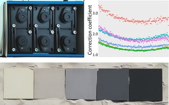
The vignette effect is a well-known phenomenon that is visible in flat field images as the light intensity falloff from the center to the edge (Figure 7). It is the percentage decrease in the illumination level reaching the focal sensor that is composed of the cosine of the fourth falloff (unavoidable) and the field efficiency of the lens itself [50]. The nonuniform quantum efficiency is the small per pixel random variation of the collected charge of pixels under the same illumination that is introduced during the manufacturing process. It overlies the vignette effect trend [28] resulting in a bumpy surface in Figure 7. Also, dust could be present on the sensor. It occurs as a black stigma in dark image (Figure 7). These effects greatly bias the DNs, so they must be reduced.
The per-pixel vignette effect, nonuniform quantum efficiency effect and dust defects were corrected using a set of flat field noise corrected images under uniform illumination using the look-up-table (LUT) correction method. The LUT correction method is constructed on the assumption that the brightest pixels in the center are not affected by any error and they can serve as reference values for normalization. Then, the ratio of the normalized DNs to the DN of each pixel can be calculated as the vignetting correction coefficient. The correction coefficients were computed using Equation (1) [51]:
where ILUT(i, j) is the correction coefficient of the pixel at position (i, j), Iref, max is the maximum brightness value of the image and Iref (i, j) is the brightness value of pixel position (i, j). The result is a raster of per-pixel correction coefficients (Figure 7b) that, after multiplying by the field images, reduces vignetting.
ILUT(i, j) = Iref, max/Iref (i, j)
The effects of the exposure time and illumination intensity on the correction coefficients were studied using the same dataset, which was used for linearity testing. The flat field images were taken at multiple exposure times of 50, 250, 500, and 1000 μS at 10 levels of light intensity at a constant temperature of 19 °C (see Table 2). The average image was computed using a set of 10 images, which were taken for every combination of exposure time and intensity. After subtracting the corresponding dark offset image from the average flat field image, the correction coefficient images were computed. The appropriate correction image was then applied to the test image from a field experiment.
2.4.4. Atmospheric Correction
Once the sensor correction is applied to the calibration image, the atmospheric corrections can be processed. Among the different calibration methodologies, we chose a vicarious calibration based on the empirical line method [52], which is also used for UAV imaging [33,53]. The method assigns a reflectance value to each pixel that is based on the computed linear relationship between the known reflectance value of the light and the dark reflectance panels (see Figure 5) and their DN numbers that were extracted from images. In general, the calibration targets should be 10+ times bigger than GSD to extract at least one hundred of pixel values [16,20]. This method greatly reduces both illumination and atmospheric effects, converts the DNs to reflectance and thus allows for the comparison of datasets that were collected in different seasons and light conditions [9].
2.5. Data Processing
The analytical processing of the data from the laboratory experiment and the computation of radiometric corrections were carried out in R [54] according to the methodology that was described in the previous subsections. The radiometric corrections and radiometric calibration of the field image were conducted in R too. R was used also to create graphs, calculate the descriptive statistics and conduct hypothesis testing. Prior to any processing in R, the images mages were converted from the proprietary 10-bit RAW format to a multispectral 16-bit Single-Page Tagged Image File Format (TIFF) using PixelWrench2 [55].
3. Results
3.1. Sensor Linearity
The sensor linearity was confirmed for each channel using a regression coefficient that was higher than 0.99, regardless of the irradiance and exposure time (Figure 8; Figure 9). The experiment also evaluated the efficiency of the relative exposure time setting that balanced the nonuniform relative sensitivity of sensors to monochromatic light. The channels with longer wavelengths in the NIR part of the spectrum have automatically longer exposure times. The channels are well balanced except for band 1 (550 nm) that has a shorter exposure time than it should have. This is because of the differences in the halogen light of the sphere and sunlight.
3.2. Noise Reduction
The dark offset images were computed for each combination of factors and bands of the camera. A simple visual assessment of the per-pixel noise characteristics of the dark offset average images reveals checkered patterns in bands 1–3 (a–c) (Figure 10). Bands 4–6 (d–f) contain salt-and-pepper and periodic noise, which more significantly affect the longer wavelengths. The checkered pattern is more visible in SD images because it forms squares with similar values.
An examination of the per-pixel dark offset images (average of 20 samples) reveals that the highest noise is in band 1, but band 1 has the smallest variability and a left skewed distribution (Figure 11). This is due to the strong checkered pattern that is associated with similar higher noise values. A shorter relative exposure time (0.75 of the master channel´s band 4 exposure time) has also an effect on the higher noise values. A similar distribution with a higher median and smaller variability of the noise is also Band 4, but it has no skewness. Band 4 also has a short relative exposure time under 1 (0.8 of the set exposure time). The distributions of Bands 4, 5, and 6 are symmetric since no strong pattern is presented. Bands 2 and 3, which also have checkered patterns, are also skewed in accordance with the previous results. Band 2 is skewed left too. Conversely, Band 3 is skewed right, which means that the checkered pattern is formed by pixels with lower noise values. The noise variability of Bands 2, 3, and 5 is less equal but higher compared to Bands 1 and 4 because all bands have longer relative exposure times of approximately 1 of the master channel´s band 4 exposure time. The band 6 shows the highest noise variability due to highest relative exposure time (1.3 of the master channel´s band 4 exposure time). The boxplot of Band 6 (exp. time 500 μS and temp. 27 °C) is missing because of damage to the RAW images.
Although only the average image is used to reduce the noise by subtracting it from the field images, it makes sense to calculate and examine the SD image that is calculated from the 20 samples since it represents an approximation of the remaining noise following dark offset subtraction. An examination of Figure 12 shows that the highest variability in the per-pixel SD that also has the highest median value is band 6. Conversely, the lowest variability and noise are visible in Bands 1 and 4. This is associated with the relative exposure time. The bands with longer relative exposure times have larger noise variation in single frames, which is reflected in the higher SD. The dark offset subtraction method reduces the image noise well. The residual noise remaining after noise correction is less than 1% of the dynamic range. The boxplot of Band 6 (exp. time of 500 μS and temp. of 27 °C) is missing because of the damage to the RAW images.
If we focus on the noise depending on the changing ambient temperature and exposure time, it is especially evident in Bands 2, 5, and 6 that at the same exposure time, the noise increases as the ambient temperature increases. Therefore, we studied these effects as the main user-controllable sources of noise.
We found a significant difference in the average value of the noise depending on the ambient temperature and exposure time. The ANOVA results are summarized in Table 4. Both effects were significant in every band. Therefore, it is necessary to apply a proper dark offset image that was calculated using dark images that were taken under the same conditions to the real-world image. Moreover, the interaction between factors was also significant for all bands; therefore, an interaction plot was created (Figure 13). The interactions are complicated and less significant compared to the main effects size. The positive effect of the rising ambient temperature to noise is clear and more pronounced, especially in Bands 1, 2, and 3, and in infrared Bands 5 and 6. In these bands, there has been a rapid increase of the noise in the measurements from 19° to 27° C with longer exposure times (500 and 1000 µS). The negative effect of the rising exposure time due to decreasing noise was more pronounced in Bands 1, 4 and 5. In Bands 1, 2, and 5, we could assume that the interactions were close to the additive effect of the factors.
3.3. Nonuniform Quantum Efficiency of CMOS Array and Vignetting Reduction
A visual assessment of the vignette effect showed that the vignetting structure is different for every band (Figure 14), but it is affected by the physical location of the sensors on the camera. We can see that the middle point of the falloff circle is significantly shifted down in Band 1 (c). On the opposite side, Band 4 (f) is shifted up. The middle pairs of Bands 3 and 6 (b and e) are shifted left. The left pairs of Bands 2 and 5 (a and d) are roughly centered. There are also visible stigmas in (e and f) that are caused by dust on sensors.
The vignetting radial falloff of each band is shown in Figure 15. The radial falloff rates (the shapes of the curves) reveal only minor variations between bands. These disparities are caused by the imperfections of the optical system of individual lenses and the different transmittance of each filter. Furthermore, there are major differences in the correction coefficient values. The strongest vignette effect results in the highest correction coefficients in Bands 1 and 4 followed by Bands 6, 5, 2 and 3. These differences are caused by the different points of origin of the vignetting (especially Bands 1 and 4, as shown in Figure 14). It is also clearly visible that the correction coefficient decreases in all bands as the exposure time increases, and that the values of the correcting factor at 50 μS significantly differ from the others in all bands. The variance of the individual pixel values also changes across the profile. The longer the exposure time that is used, the lower the variance. These disparities are caused mainly by the actual dynamic range of the flat field image.
The dynamic range is dependent on both the exposure time and the illumination intensity (Figure 16). The interaction plot shows the effects of the exposure time and illumination intensity on the mean correction coefficient. It is clearly visible that the mean correction coefficient decreases as the exposure time increases and the illumination is stronger since both factors influence the dynamic range that is stored in the flat field. A short exposure time combined with the low light intensity limit the dynamic range, resulting in a higher mean value of the correction coefficient.
The results of the laboratory experiment show that the value of the correction factor is dependent on the selected exposure time and actual light intensity. Therefore, it is necessary to apply a proper vignetting correction coefficient array to the real-world image, which was calculated from the flat field images that were taken in the same conditions.
3.4. Results of Field Experiment
The effect of the proposed correction workflow was first investigated using a randomly selected profile (red line in Figure 5) to compare the normalized DNs of the raw and corrected images of the profile (Figure 17) and the distribution of the values (Figure 18). The original profile reveals a strong decrease of the DNs that is caused by the vignette effect. Conversely, the normalized DNs show no decrease or only a slight decrease. If we compare the Coefficients of Variation of the profiles, we can see that there is a significant reduction in the variation from 50% to 70% after correction occurs. To prove this hypothesis, we performed the Fligner-Killeen scale test with the null hypothesis that the variation ratio of the original and corrected DNs is less or equal than 1. I.e., the numerator (variation of the original DNs) would have to be bigger than the denominator (the variation of the normalized DNs) (Table 5). The result showed that the variation of the DNs that are extracted from the corrected image is significantly smaller than that from the original image. In addition, there is also a visible reduction in DNs errors that is caused by random nonuniform quantum efficiency (Figure 17).
The main practical result of this study is the confirmation that the proposed calibration workflow significantly restored the surface reflectance compared to a field measurement, as shown in Figure 19. Figure 19 compares the three validation target reflectance curves that are derived from the spectrometer measurement using the median reflectance values of the same targets that are extracted from the raw (red dots) and corrected (green dots) images.
The greatest improvement occurs, as expected at Target 4, due to the strongest vignette effect resulting from its location in the selected field image (see Figure 5). While the raw image reflectance values are below 0.35, the corrected reflectance values strongly respond with reflectance curve values of approximately 0.40. A similar improvement in the reflectance values after applying all corrections occurs also in the case of Target 7 with the exception that there is not such a strong vignette effect at the target as in Target 4; therefore, the reflectance improves from 0.01 to 0.03. Another reason is the dynamic range, which is lower in the case of dark targets than in the case of light ones. In the case of Target 5, the improvement is not as large because the target is closest to the center and the vignetting effect is not as pronounced.
If we compare the NRMSE values between the raw and corrected images, we can see that the values for Target 4 are ten times lower in the corrected image (Table 6). The NRMSE values of Target 7 are 2-10 times lower in the corrected image. The greatest improvement was achieved for more distant targets where the vignetting effect was the strongest. These results confirm the high efficiency of the proposed correction procedure resulting in excellent coherence between the reflectance of the verification targets between the reference field measurement and the fully radiometrically and atmospherically corrected image.
4. Discussion
To achieve the proper spectral image properties and retain the consistency across multispectral UAV imaging campaigns, the application of the appropriate radiometric and atmospheric corrections is a necessary prerequisite. Due to the limited or lacking calibration protocols and information on the sensor’s radiometric properties (linear response, vignetting and the signal-to-noise ratio), the growing variety of UAV sensors and the customization of their spectral bands using interchangeable filters, the development of a reliable radiometric correction method that is applicable in conditions of field imaging campaigns is important both for research and practical applications.
Increasing number of multispectral sensors and growing volumes of imagery, acquired by different sensors underlines the importance of achieving comparability across the sensors and acquisition conditions [20]. For this purpose, an open workflow for transparent calculation of radiometric corrections, enabling comparison and use of the imagery acquired by different sensors, is of growing importance and is applicable also to the sensors, featuring auto-calibration routines such as Parrot Sequoia or MicaSense RedEdge.
In this study, we have proposed and tested a reliable calibration workflow enabling straightforward empirical, image-based radiometric corrections combined with vicarious atmospheric correction using the empirical line approach. The workflow comprises techniques that reduce noise, lens vignetting and nonuniform quantum efficiency of the CMOS array. The sensor corrections (noise and vignetting reduction) should be applied prior any photogrammetric processing. The atmospheric corrections can be performed apriori to processing, or during processing using tools implemented to the photogrammetric software. This approach was tested on the Tetracam uMCA sensor with customizable spectral bands. The achieved results are related to this particular sensor, however the workflow was designed to be reproducible and applicable to the other types of multispectral multiframe systems with CCD/CMOS sensors and global shutters as well, such as Parrot Sequoia and MicaSense RedEdge. Every step of the proposed workflow can be used as it is designed for if another camera has monochrome frame sensors with global shutter and the linear response to incoming light. If the sensors have a rolling shutter, the additional source of noise should be considered [34]. The sensor linearity is also an underlying assumption of using empirical line atmospheric correction with two targets. When the camera does not have a linear response, modified empirical methods using more than two targets have to be applied. This occurs in the study of Wang and Myint [56], which used nine shades of gray to model the exponential relationship of a modified color infrared single-lens reflex camera.
The key reason for selecting Tetracam camera for our research was its relevance to our research aims, namely its ability to provide a set of relatively narrow spectral bands, configured according to the needs of our research tasks. In particular, for our research, there is beneficial ability of the sensor to split the near-infrared light into several narrow spectral bands. To the contrary, the other popular global shutter multispectral cameras, as MicaSense RedEdge or Parrot Sequoia have fixed configuration of spectral bands, not allowing customization according to the research needs.
The linear response of the camera to incoming light was examined first. It was important to carry out a complex experiment assessing various relevant exposure times and sunlight intensities to check the stability of the radiometric response due to the variation of the camera’s radiometric properties [53]. In the experiment that was performed in this study, the sensor’s linearity was established. This confirmed the appropriate setting of the relative exposure time compensating for the sensors’ nonuniform relative sensitivity to the light and the nonuniform filter transmittance of the individual bands, except for Band 1. The reason is the radiance difference in the halogen light of the sphere and sunlight. While sunlight has a maximum radiance of approximately 500 nm, the sphere light has a maximum radiance of 900 nm. That is why exposure time of Band 1 (550 nm) is underestimated.
A visual assessment of the per-pixel noise characteristics of the dark offset samples revealed the checkered pattern on Bands 1–3, which is apparent both in all the averaged datasets and in the single images. Since there was no natural explanation for the phenomenon, we inquired with the camera’s manufacturer on the occurrence of the patterns. According to the manufacturer, this moire pattern is a product of the rotation and scaling of slave images relative to master images (Band 4) and each other. The moire pattern occurred when converting images from the RAW format to TIFF in PixelWrench 2, which is the system software that was provided by the sensor manufacturer. Therefore, the moire pattern is present in each frame, as a constant noise pattern in addition to random thermal noise. The testing of the correction workflow thus disclosed the undesired and undocumented effects of the sensor array. Although Kelcey and Lucieer [34] state that dark offset subtraction is limited when reducing this effect, the camera manufacturer nevertheless considers it as an appropriate method for reducing the moire pattern.
The vignette effect analysis showed that the vignetting structure acts differently in the sensor array. The central point of the falloff circle is shifted for every band. The central point is shifted the most in Band 1, which also explains the significantly higher vignetting corrections on the selected transverse profile. In addition, it was discovered that the maximum values of the correcting factors for Bands 2, 3, and 6 were over 100. We have revealed that these values are present only on the last edge line of the pixels of each picture and are a product of the defective cells of the CMOS chip. The black stigma in master channel Band 4 (Figure 7) is the dust on sensor that could not be removed by user, but it could be corrected using LUT correction method. The filter that produces the greatest numbers of electrons in response to the radiation is then by the manufacturer selected as master filter/channel [15]. The similar spot artifacts on the imagery were, indeed, reported as dust particles on chip by Kelcey and Lucieer [34]. The potential impact of removable dust was eliminated by cleaning lenses before each use and by keeping the integration sphere tidy.
In addition to previous studies, the radiometric corrections were performed in varying controlled laboratory conditions to simulate the most typical natural conditions during imaging, and the variation of the camera’s radiometric properties was assumed to be due to inexpensive sensors. The results of the laboratory experiment revealed that the noise distribution significantly varied depending on the exposure time and the ambient temperature. The exposure time should be considered to be the main interior user-controllable source of thermal noise because the aperture value is fixed (f/3.2). The ambient temperature could be considered as the main external independent source of thermal noise, which is consistent with the experiments using hyperspectral sensors in [16,43,44]. Moreover, the noise distribution’s characteristics were significantly different in each band due to the relative exposure settings of the camera. If we compare the SDs, which represented approximations of the remaining noise following dark offset subtraction, we can conclude that the best results are achieved in the bands with relatively shorter exposure times resulting in less random noise.
The vignetting correction coefficient values have been shown to vary depending on the exposure time and the intensity of the incident radiation. A short exposure time and/or low light intensity reduce the dynamic range, resulting in the presence of extremely low values and their increased frequency in proportion to the maximum value. This results in an increase in both the maximum and mean values of the calculated vignetting correction coefficient (see Figure 15; Figure 16). This finding makes the noise reduction methods for dark offset images and the vignetting correction methods for LUT tables less applicable, although the methods themselves may be suitable for reducing these undesirable effects [44,53]. The main principles of both methods are calculating a database of correction images in the laboratory and then applying the correction images that were taken in the same conditions as during flight. For this solution, however, it is necessary to build a large database of correction pictures for all combinations of relevant exposures, ambient temperatures and light intensities, resulting in hundreds of correction images and thousands of input images for calculating the corrections, which is truly time and storage consuming.
Simultaneously, it is still necessary to measure the ambient temperature using an on-board thermologger and the irradiance using an on-board or field sensor to determine the correct intensity of the calibration sphere [57,58], which requires further equipment investments. An alternative to this approach would be to acquire a set of correction pictures in the field. Dark images could be taken in a black box and vignetting correction images could be generated by capturing photos of spectrally homogeneous panels under the same illumination. However, only a few authors have addressed this. Aasen et al. [16] and Yang et al. [53] included in situ flat field vignetting calibration into the processing chain because the results were comparable with laboratory calibrations. Crusiol et al. [17] compare the laboratory and field calibrations of a modified color infrared single-lens reflex camera, but without noise removal. The results look promising with a correlation coefficient of R2 > 0.9 that was found for the cross calibration (laboratory vs field).
Calibration images for the vicarious calibration can be collected before and after flight from ground, or during the flight [20]. The common practice is to take one calibration image before and after the flight from drone and sensor held manually above the target with MicaSense RedEdge or Parrot Sequoia [18,19]. However, such approaches are usually simplified, and atmospheric effects are not reduced [10]. On the other side, the in-flight calibration, where calibration targets are taken from the flight altitude, reduce the atmospheric effects
In this field experiment, the flight altitude was set to fit the size of the court that defined the distribution of the targets. The experiment was designed to demonstrate the main radiometric issues (noise and vignetting) of frame multispectral cameras, which alter the DN numbers and derived reflectance values in every single image. If these effects are not reduced in every image, the resulting reflectance mosaic used for analysis is biased. To demonstrate these effects, we used the single image, but with raw and corrected DN values to avoid additional effects of mosaicking (blending the DN values around seamlines) and to preserve the pure effect of vignetting. The similar approach was used in previous works [17,35,36].We performed the field experiment comparing the reflectance values of three validation targets distributed in the corners, where the vignette effect is the strongest.
The results of the field experiment confirmed the general assumption that the greatest impact on overall accuracy is the removal of vignetting, which is consistent with the statement of Lebourgeois et al. [59]. The vignetting correction using the LUT method, which is the most for precise application compared to the optical modeling method [51], significantly reduced the diagonal profile variance. The Coefficient of variation decreased by half in all bands and the DNs were equalized. A similar decrease of the CV was achieved by calibrating a spaceborne linear scanner using a CCD chip [28]. The application of atmospheric calibration to normalized DNs resulted in a significantly more accurate determination of the reflectance of the three validation targets compared to the raw data, thus improving the NRMSE. The NRMSEs after processing all corrections ranged from 0.24 to 2.10%, which are comparable with the results of Del Pozo et al. [36] (2%), Aasen et al. [16] (1%), and Yang et al. [53] (5%). The results, which were verified using a field experiment, demonstrated that the proposed correction workflow significantly improves the quality of multispectral imagery.
In the main field experiment, the calibration targets were placed in the field center in order to minimize the influence of vignetting in the raw and calibrated images. However, the calibration targets are not always located in the center of the calibration image during a field campaign but can be shifted to the edges. Hence, an additional experiment was conducted for this reason when the location effect of the calibration targets on radiometric corrections was considered. We used the Pearl 4 and Medium Gray 7 targets that were located close to the outer edge as the calibration targets and the remaining Cream 1, Light Gray 5 and Anthracite 9 targets were used as validation targets. The separate linear relationship between the DN and reflectance was computed for every channel of the raw and radiometrically corrected images. The results of this experiment are shown in Figure 20. In this case, the vignetting corrections have an even greater effect on the accuracy of the radiometric calibration comparing raw and corrected images. If the calibration targets are placed on the edges without vignetting corrections, their DNs are strongly underestimated. Calculating an empirical line using these underestimated values then leads to a strong overestimation of the reflectance values for the validation targets (dark red dots in Figure 20). The more biased values are obtained from the center targets of Cream 1 (b) and Anthracite 9 (c) where the vignetting effect is low. In the case of the Light Gray 5 target (a), a comparison of the location effect can be made. Slightly more accurate results are obtained when calibration targets are placed in the center. In addition, the bias of the raw reflectance values completely degrades the data quality when the calibration targets are placed close to an edge.
5. Conclusions
This study proposed and tested a complex empirical image-based radiometric calibration and atmospheric correction method for a Tetracam μMCA multispectral frame camera with a global shutter. Our proposed correction workflow comprises techniques for reducing noise, lens vignetting, and nonuniform quantum efficiency of the CMOS array, which extends the previous works on the calibration of older camera models with rolling shutters by adopting the calibration experiments to hyperspectral sensors. The workflow is based on a laboratory investigation of the camera’s radiometric properties combined with vicarious atmospheric correction using an empirical line. The effect of the corrections, which were demonstrated using out-of-laboratory field data, proved the substantial effect of the corrections.
Sensor linearity was confirmed for each channel with coefficients of correlated greater than 0.999, regardless of the irradiance and exposure time. The dark signal noise behaviour was investigated based on the exposure time and ambient temperature and the vignette effect coupled with nonuniform quantum efficiency was studied for changing exposure times and illumination to simulate real-world conditions. In both cases, there was a strong dependence on the exposure time, ambient temperature and illumination.
The results of the field experiment confirmed the general assumption that the greatest impact on the overall accuracy is the reduction of vignetting. The vignetting correction using the LUT method resulted in a significant reduction of the diagonal profile variance, thereby decreasing the Coefficient of variation by half in all bands and overall equalizing the DNs. The application of atmospheric calibration to normalized DNs led to a significantly more accurate determination of the reflectance of the three validation targets compared to the raw data and resulted in the improvement of the NRMSE by an order of magnitude. The NRMSEs after processing all corrections ranged from 0.24 to 2.10%, which demonstrates that the correction procedure is well designed to calibrate multispectral frame cameras.
The presented workflow showed the efficiency of the method by increasing the accuracy of the determination of the reflectance from UAV multispectral imagery, which is a key for the reliability and reproducibility of imaging results. Meanwhile, it demonstrated its practical applicability in conditions of field campaigns and the approach is applicable to other multiarray imaging systems that equipped with CCD/CMOS sensors and global shutters.
Author Contributions
R.M. designed the research, conducted laboratory and field experiments, collected data, analysed data and prepared the manuscript. J.L. supervised the study, contributed in field experiment, reviewed and edited the manuscript and J.H. contributed in laboratory experiment and data processing.
Funding
The study was supported by the Charles University, project GA UK No. 824217 “Analysis of disturbance and regeneration of forest vegetation using UAV multispectral photogrammetry” and COST Action CA16219—Harmonization of UAS techniques for agricultural and natural ecosystems monitoring.
Acknowledgments
The authors would like to thank Daniel Žížala for his statistical computation support and Theodora Lendzioch for her help in the field.
Conflicts of Interest
The authors declare no conflict of interest.
References
- Salamí, E.; Barrado, C.; Pastor, E. UAV flight experiments applied to the remote sensing of vegetated areas. Remote Sens. 2014, 6, 11051–11081. [Google Scholar] [CrossRef]
- Candiago, S.; Remondino, F.; De Giglio, M.; Dubbini, M.; Gattelli, M. Evaluating Multispectral Images and Vegetation Indices for Precision Farming Applications from UAV Images. Remote Sens. 2015, 7, 4026–4047. [Google Scholar] [CrossRef] [Green Version]
- Torresan, C.; Berton, A.; Carotenuto, F.; Di Gennaro, S.F.; Gioli, B.; Matese, A.; Miglietta, F.; Vagnoli, C.; Zaldei, A.; Wallace, L. Forestry applications of UAVs in Europe: A review. Int. J. Remote Sens. 2017, 38, 2427–2447. [Google Scholar] [CrossRef]
- Adão, T.; Hruška, J.; Pádua, L.; Bessa, J.; Peres, E.; Morais, R.; Sousa, J. Hyperspectral Imaging: A Review on UAV-Based Sensors, Data Processing and Applications for Agriculture and Forestry. Remote Sens. 2017, 9, 1110. [Google Scholar] [CrossRef]
- Pádua, L.; Vanko, J.; Hruška, J.; Adão, T.; Sousa, J.J.; Peres, E.; Morais, R. UAS, sensors, and data processing in agroforestry: A review towards practical applications. Int. J. Remote Sens. 2017, 38, 2349–2391. [Google Scholar] [CrossRef]
- Zhang, C.; Kovacs, J.M. The application of small unmanned aerial systems for precision agriculture: A review. Precis. Agric. 2012, 13, 693–712. [Google Scholar] [CrossRef]
- Näsi, R.; Honkavaara, E.; Lyytikäinen-Saarenmaa, P.; Blomqvist, M.; Litkey, P.; Hakala, T.; Viljanen, N.; Kantola, T.; Tanhuanpää, T.; Holopainen, M. Using UAV-based photogrammetry and hyperspectral imaging for mapping bark beetle damage at Tree-Level. Remote Sens. 2015, 7, 15467–15493. [Google Scholar] [CrossRef]
- Aasen, H.; Honkavaara, E.; Lucieer, A.; Zarco-Tejada, P.J. Quantitative remote sensing at Ultra-High resolution with UAV spectroscopy: A review of sensor technology, measurement procedures, and data correctionworkflows. Remote Sens. 2018, 10, 1091. [Google Scholar] [CrossRef]
- Smith, G.M.; Milton, E.J. The use of the empirical line method to calibrate remotely sensed data to reflectance. Int. J. Remote Sens. 1999, 20, 2653–2662. [Google Scholar] [CrossRef]
- Aspinall, R.J.; Marcus, W.A.; Boardman, J.W. Considerations in collecting, processing, and analysing high spatial resolution hyperspectral data for environmental investigations. J. Geogr. Syst. 2002, 4, 15–29. [Google Scholar] [CrossRef]
- Sandau, R.; Beisl, U.; Braunecker, B.; Cramer, M.; Driescher, H.; Eckardt, A.; Fricker, P.; Gruber, M.; Hilbert, S.; Jacobsen, K.; et al. Digital Airborne Camera: Introduction and Technology; Sandau, R., Ed.; Springer: Dordrecht, The Netherlands, 2010; ISBN 9781402088773. [Google Scholar]
- Ryan, R.E.; Pagnutti, M. Enhanced absolute and relative radiometric calibration for digital aerial cameras. In Proceedings of the Photogrammetric Week’09; Fritch, D., Ed.; Wichtmann Verlag: Heidelberg, Germany, 2009; pp. 81–90. [Google Scholar]
- Gao, B.C.; Montes, M.J.; Davis, C.O.; Goetz, A.F.H. Atmospheric correction algorithms for hyperspectral remote sensing data of land and ocean. Remote Sens. Environ. 2009, 113, 16–24. [Google Scholar] [CrossRef]
- Dinguirard, M.; Slater, P.N. Calibration of Space-Multispectral imaging sensors: A review. Remote Sens. Environ. 1999, 68, 194–205. [Google Scholar] [CrossRef]
- Tetracam Inc. Tetracam µMCA User’s Guide. Available online: http://www.tetracam.com/PDFs/u%20MCA%20Users%20Guide%20V1.1.pdf (accessed on 17 August 2019).
- Aasen, H.; Burkart, A.; Bolten, A.; Bareth, G. Generating 3D hyperspectral information with lightweight UAV snapshot cameras for vegetation monitoring: From camera calibration to quality assurance. ISPRS J. Photogramm. Remote Sens. 2015, 108, 245–259. [Google Scholar] [CrossRef]
- Crusiol, L.G.T.; Nanni, M.R.; Silva, G.F.C.; Furlanetto, R.H.; da Silva Gualberto, A.A.; de Carvalho Gasparotto, A.; De Paula, M.N. Semi professional digital camera calibration techniques for Vis/NIR spectral data acquisition from an unmanned aerial vehicle. Int. J. Remote Sens. 2017, 38, 2717–2736. [Google Scholar] [CrossRef]
- Parrot. Parrot Announcement-Release of Application Notes. Available online: https://forum.developer.parrot.com/t/parrot-announcement-release-of-application-notes/5455 (accessed on 27 September 2019).
- MicaSense. Best Practices: Collecting Data with MicaSense Sensors. Available online: http://support.micasense.com/hc/en-us/articles/224893167-Best-practices-Collecting-Data-with-MicaSense-RedEdge-and-Parrot-Sequoia (accessed on 27 September 2019).
- Assmann, J.J.; Kerby, J.T.; Cunliffe, A.M.; Myers-Smith, I.H. Vegetation monitoring using multispectral sensors—Best practices and lessons learned from high latitudes. J. Unmanned Veh. Syst. 2018, 7, 54–75. [Google Scholar] [CrossRef]
- Withagen, P.J.; Groen, F.C.A.; Schutte, K. CCD color camera characterization for image measurements. IEEE Trans. Instrum. Meas. 2007, 56, 199–203. [Google Scholar] [CrossRef]
- Healey, G.E.; Kondepudy, R. Radiometric CCD camera calibration and noise estimation. IEEE Trans. Pattern Anal. Mach. Intell. 1994, 16, 267–276. [Google Scholar] [CrossRef]
- Mullikin, J.C.; van Vliet, L.J.; Netten, H.; Boddeke, F.R.; van der Feltz, G.; Young, I.T. Methods for CCD Camera Characterization. In Proceedings of the Image Acquisition and Scientific Imaging Systems; Titus, H.C., Waks, A., Eds.; International Society for Optics and Photonics: San Jose, CA, USA, 1994; Volume 2173, pp. 73–84. [Google Scholar]
- Fraser, C.S. Digital camera Self-Calibration. ISPRS J. Photogramm. Remote Sens. 1997, 52, 149–159. [Google Scholar] [CrossRef]
- Hytti, H.T. Characterization of digital image noise properties based on RAW data. Electron. Imaging 2006, 6059, 60590A. [Google Scholar]
- Neale, C.M.U.; Crowther, B.G. An airborne multispectral video/radiometer remote sensing system: Development and calibration. Remote Sens. Environ. 1994, 49, 187–194. [Google Scholar] [CrossRef]
- Mansouri, A.; Marzani, F.S.; Gouton, P. Development of a Protocol for CCD Calibration: Application to a Multispectral Imaging System. Int. J. Robot. Autom. 2005, 20. [Google Scholar] [CrossRef] [Green Version]
- Olsen, D.; Dou, C.; Zhang, X.; Hu, L.; Kim, H.; Hildum, E. Radiometric calibration for AgCam. Remote Sens. 2010, 2, 464–477. [Google Scholar] [CrossRef]
- Hunt, E.R.; Dean Hively, W.; Fujikawa, S.J.; Linden, D.S.; Daughtry, C.S.T.; McCarty, G.W. Acquisition of NIR-Green-Blue digital photographs from unmanned aircraft for crop monitoring. Remote Sens. 2010, 2, 290–305. [Google Scholar] [CrossRef]
- Lehmann, J.; Nieberding, F.; Prinz, T.; Knoth, C. Analysis of Unmanned Aerial System-Based CIR Images in Forestry—A New Perspective to Monitor Pest Infestation Levels. Forests 2015, 6, 594–612. [Google Scholar] [CrossRef]
- Minařík, R.; Langhammer, J. Use of a multispectral UAV photogrammetry for detection and tracking of forest disturbance dynamics. In Proceedings of the International Archives of the Photogrammetry, Remote Sensing and Spatial Information Sciences; Halounova, L., Ed.; Copernicus GmbH: Göttingen, Gemany, 2016; Volume XLI-B8, pp. 711–718. [Google Scholar]
- Lelong, C.C.D.; Burger, P.; Jubelin, G.; Roux, B.; Labbé, S.; Baret, F. Assessment of unmanned aerial vehicles imagery for quantitative monitoring of wheat crop in small plots. Sensors 2008, 8, 3557–3585. [Google Scholar] [CrossRef]
- Berni, J.A.J.; Zarco-tejada, P.P.J.; Suarez, L.; Fereres, E.; Member, S.; Suárez, L. Thermal and Narrowband Multispectral Remote Sensing for Vegetation Monitoring From an Unmanned Aerial Vehicle. IEEE Trans. Geosci. Remote Sens. 2009, 47, 722–738. [Google Scholar] [CrossRef] [Green Version]
- Kelcey, J.; Lucieer, A. Sensor correction of a 6-Band multispectral imaging sensor for UAV remote sensing. Remote Sens. 2012, 4, 1462–1493. [Google Scholar] [CrossRef]
- Kelcey, J.; Lucieer, A. Sensor Correction and Radiometric Calibration of a 6-Band Multispectral Imaging Sensor for Uav Remote Sensing. ISPRS-Int. Arch. Photogramm. Remote Sens. Spat. Inf. Sci. 2012, XXXIX-B1, 393–398. [Google Scholar] [CrossRef]
- Del Pozo, S.; Rodríguez-Gonzálvez, P.; Hernández-López, D.; Felipe-García, B. Vicarious radiometric calibration of a multispectral camera on board an unmanned aerial system. Remote Sens. 2014, 6, 1918–1937. [Google Scholar] [CrossRef]
- Nocerino, E.; Dubbini, M.; Menna, F.; Remondino, F.; Gattelli, M.; Covi, D. Geometric calibration and radiometric correction of the maia multispectral camera. In Proceedings of the International Archives of the Photogrammetry, Remote Sensing and Spatial Information Sciences; Honkavaara, E., Ed.; Copernicus GmbH: Göttingen, Germany, 2017; Volume XLII-3/W3, pp. 149–156. [Google Scholar]
- Padró, J.-C.; Muñoz, F.-J.; Ávila, L.; Pesquer, L.; Pons, X. Radiometric Correction of Landsat-8 and Sentinel-2A Scenes Using Drone Imagery in Synergy with Field Spectroradiometry. Remote Sens. 2018, 10, 1687. [Google Scholar] [CrossRef]
- Padró, J.-C.; Carabassa, V.; Balagué, J.; Brotons, L.; Alcañiz, J.M.; Pons, X. Monitoring opencast mine restorations using Unmanned Aerial System (UAS) imagery. Sci. Total Environ. 2019, 657, 1602–1614. [Google Scholar] [CrossRef] [PubMed]
- Honkavaara, E.; Saari, H.; Kaivosoja, J.; Pölönen, I.; Hakala, T.; Litkey, P.; Mäkynen, J.; Pesonen, L. Processing and Assessment of Spectrometric, Stereoscopic Imagery Collected Using a Lightweight UAV Spectral Camera for Precision Agriculture. Remote Sens. 2013, 5, 5006–5039. [Google Scholar] [CrossRef] [Green Version]
- Hakala, T.; Honkavaara, E.; Saari, H.; Mäkynen, J.; Kaivosoja, J.; Pesonen, L.; Pölönen, I. Spectral imaging from UAVs under varying illumination conditions. In Proceedings of the International Archives of the Photogrammetry, Remote Sensing and Spatial Information Sciences; Grenzdörffer, G., Bill, R., Eds.; Copernicus GmbH: Göttingen, Germany, 2013; Volume XL-1/W2, pp. 189–194. [Google Scholar]
- Hruska, R.; Mitchell, J.; Anderson, M.; Glenn, N.F. Radiometric and geometric analysis of hyperspectral imagery acquired from an unmanned aerial vehicle. Remote Sens. 2012, 4, 2736–2752. [Google Scholar] [CrossRef]
- Aasen, H.; Bendig, J.; Bolten, A.; Bennertz, S.; Willkomm, M.; Bareth, G. Introduction and preliminary results of a calibration for full-frame hyperspectral cameras to monitor agricultural crops with UAVs. In Proceedings of the International Archives of the Photogrammetry, Remote Sensing and Spatial Information Sciences; Sunar, F., Altan, O., Taberner, M., Eds.; Copernicus GmbH: Göttingen, Gemany, 2014; Volume XL–7, pp. 1–8. [Google Scholar]
- Buettner, A.; Roeser, H.P. Hyperspectral remote sensing with the UAS “Stuttgarter adler”—Challenges, experiences and first results. In Proceedings of the International Archives of the Photogrammetry, Remote Sensing and Spatial Information Sciences; Grenzdörffer, G., Bill, R., Eds.; Copernicus GmbH: Göttingen, Germany, 2013; Volume XL-1/W2, pp. 61–65. [Google Scholar]
- Suomalainen, J.; Anders, N.; Iqbal, S.; Roerink, G.; Franke, J.; Wenting, P.; Hünniger, D.; Bartholomeus, H.; Becker, R.; Kooistra, L. A lightweight hyperspectral mapping system and photogrammetric processing chain for unmanned aerial vehicles. Remote Sens. 2014, 6, 11013–11030. [Google Scholar] [CrossRef]
- Baugh, W.M.; Groeneveld, D.P. Empirical proof of the empirical line. Int. J. Remote Sens. 2008, 29, 665–672. [Google Scholar] [CrossRef]
- Al-Amri, S.S.; Kalyankar, N.V.; Santosh, K. A Comparative Study of Removal Noise from Remote Sensing Image. Int. J. Comput. Sci. Issues 2010, 7, 32–36. [Google Scholar]
- Box, G.E.P.; Cox, D.R. An Analysis of Transformations. J. R. Stat. Soc. Ser. B 1964, 26, 211–252. [Google Scholar] [CrossRef]
- Greenhouse, S.W.; Geisser, S. On methods in the analysis of profile data. Psychometrika 1959, 24, 95–112. [Google Scholar] [CrossRef]
- Goldman, D.B. Vignette and Exposure Calibration and Compensation. IEEE Trans. Pattern Anal. Mach. Intell. 2010, 32, 2276–2288. [Google Scholar] [CrossRef]
- Yu, W. Practical Anti-Vignetting methods for digital cameras. IEEE Trans. Consum. Electron. 2004, 50, 975–983. [Google Scholar]
- Teillet, P.M. Image correction for radiometric effects in remote sensing. Int. J. Remote Sens. 1986, 7, 1637–1651. [Google Scholar] [CrossRef]
- Yang, G.; Li, C.; Wang, Y.; Yuan, H.; Feng, H.; Xu, B.; Yang, X. The DOM generation and precise radiometric calibration of a UAV-Mounted miniature snapshot hyperspectral imager. Remote Sens. 2017, 9, 642. [Google Scholar] [CrossRef]
- R Core Team. R: A Language and Environment for Statistical Computing; R Foundation for Statistical Computing: Vienna, Austria; Available online: http://www.R-project.org/ (accessed on 21 January 2018).
- Tetracam Inc. PixelWrench2 User Guide. Available online: http://www.tetracam.com/PDFs/Tetracam_PixelWrench2_User_Guide.pdf (accessed on 21 January 2018).
- Wang, C.; Myint, S.W. A Simplified Empirical Line Method of Radiometric Calibration for Small Unmanned Aircraft Systems-Based Remote Sensing. IEEE J. Sel. Top. Appl. Earth Obs. Remote Sens. 2015, 8, 1876–1885. [Google Scholar] [CrossRef]
- Nevalainen, O.; Honkavaara, E.; Tuominen, S.; Viljanen, N.; Hakala, T.; Yu, X.; Hyyppä, J.; Saari, H.; Pölönen, I.; Imai, N.; et al. Individual Tree Detection and Classification with UAV-Based Photogrammetric Point Clouds and Hyperspectral Imaging. Remote Sens. 2017, 9, 185. [Google Scholar] [CrossRef]
- Tuominen, S.; Balazs, A.; Honkavaara, E.; Pölönen, I.; Saari, H.; Hakala, T.; Viljanen, N. Hyperspectral UAV-Imagery and photogrammetric canopy height model in estimating forest stand variables. Silva Fenn. 2017, 51, 7721. [Google Scholar] [CrossRef]
- Lebourgeois, V.; Bégué, A.; Labbé, S.; Mallavan, B.; Prévot, L.; Roux, B. Can Commercial Digital Cameras Be Used as Multispectral Sensors? A Crop Monitoring Test. Sensors 2008, 8, 7300–7322. [Google Scholar] [CrossRef]
Figure 1.
Multispectral 6-channel camera Tetracam uMCA Snap 6 equipped with 6 1.3 mega-pixel complementary metal oxide semiconductor (CMOS) sensors and changeable bandpass filters. This filter set includes 550 nm, 650 nm, 700 nm, 800 nm, 850 nm, 900 nm filter with FWHM 20 mm.
Figure 1.
Multispectral 6-channel camera Tetracam uMCA Snap 6 equipped with 6 1.3 mega-pixel complementary metal oxide semiconductor (CMOS) sensors and changeable bandpass filters. This filter set includes 550 nm, 650 nm, 700 nm, 800 nm, 850 nm, 900 nm filter with FWHM 20 mm.

Figure 2.
The full data processing workflow proposed in this study to create a reflectance data product.
Figure 2.
The full data processing workflow proposed in this study to create a reflectance data product.

Figure 3.
CSTM-LR-20-M integrating sphere with mounted multispectral camera above in the dark room.

Figure 4.
CSTM-LR-20-M integrating sphere spectral radiance curve from 300 nm to 2500 nm with maximum radiance around 900 nm.
Figure 4.
CSTM-LR-20-M integrating sphere spectral radiance curve from 300 nm to 2500 nm with maximum radiance around 900 nm.

Figure 5.
(a) The design of the field experiment. The single image in sensor geometry with the ground sampling distance (GSD) of 0.75 cm was used for the analysis. Figure shows the distribution of calibrating (1, 9) and validation (4, 5, 7) targets. Red line marks the profile to test the hypothesis that the variation of pixels along profile extracted from original non-corrected image is greater than the variation of pixels extracted from correction image. Red squares mark the validation targets; (b) The detailed view on targets.

Figure 6.
The reflectance of targets used in the field experiment measured by StellarNet BlueWAVE field spectrometer directly before flight.
Figure 6.
The reflectance of targets used in the field experiment measured by StellarNet BlueWAVE field spectrometer directly before flight.

Figure 7.
(a) 3D Illustration of vignette effect and flat field image with typical light falloff and bumpy surface caused by nonuniform quantum efficiency in Channel 4; (b) corresponding correction coefficient image. The black stigma in (a) is the dust on sensor itself that could not be removed by user, but it could be corrected using look-up-table (LUT) correction method (b).

Figure 8.
The linear response of the camera at different exposure times: (a) Exposure time 50 µS; (b) Exposure time 250 µS; (c) Exposure time 500 µS; (d) Exposure time 1000 µS. The sensor linearity was confirmed on each channel with a regression coefficient higher than 0.99.
Figure 8.
The linear response of the camera at different exposure times: (a) Exposure time 50 µS; (b) Exposure time 250 µS; (c) Exposure time 500 µS; (d) Exposure time 1000 µS. The sensor linearity was confirmed on each channel with a regression coefficient higher than 0.99.

Figure 9.
The linear response of the camera at 40% of the integrating sphere source maximum intensity.
Figure 9.
The linear response of the camera at 40% of the integrating sphere source maximum intensity.

Figure 10.
Dark offset imagery taken at a temperature 8 °C, exposure time 500μS of all bands: (a) Average image B1; (b) Average image B2; (c) Average image B3; (d) Average image B4; (e) Average image B5; (f) Average image B6; (g) Standard deviation image B1; (h) Standard deviation image B2; (i) Standard deviation image B3; (j) Standard deviation image B4; (k) Standard deviation image B5; (l) Standard deviation image B6. The average and standard deviation (SD) images are calculated from 20 samples.


Figure 11.
Comparison of the per-pixel noise distribution of dark offset images in the laboratory experiment: (a) Exposure time 50 µS; (b) Exposure time 250 µS; (c) Exposure time 500 µS; (d) Exposure time 1000 µS.
Figure 11.
Comparison of the per-pixel noise distribution of dark offset images in the laboratory experiment: (a) Exposure time 50 µS; (b) Exposure time 250 µS; (c) Exposure time 500 µS; (d) Exposure time 1000 µS.

Figure 12.
Comparison of the per-pixel SD noise characteristics divided by exposure time: (a) Exposure time 50 µS; (b) Exposure time 250 µS; (c) Exposure time 500 µS; (d) Exposure time 1000 µS.
Figure 12.
Comparison of the per-pixel SD noise characteristics divided by exposure time: (a) Exposure time 50 µS; (b) Exposure time 250 µS; (c) Exposure time 500 µS; (d) Exposure time 1000 µS.

Figure 13.
The interaction plot of model term temp:exptime for each band: (a) Band 1; (b) Band 2; (c) Band 3; (d) Band 4; (e) Band 5; (f) Band 6. Error bars represent 95% confidence intervals.
Figure 13.
The interaction plot of model term temp:exptime for each band: (a) Band 1; (b) Band 2; (c) Band 3; (d) Band 4; (e) Band 5; (f) Band 6. Error bars represent 95% confidence intervals.

Figure 14.
The vignette effect of μMCA camera channels: (a) Band 5; (b) Band 6; (c) Band 1; (d) Band 2; (e) Band 3; (f) Band 4 (Master). The order of channels is in consistent with physical location of sensors on the camera. The red arrow marks a vignetting profile where correction coefficients were subjected to further investigation for each. Profile starts in upper right corner and ends in lower left corner.

Figure 15.
The vignetting radial falloff of each band at the 40% of the integrating sphere source maximum intensity: (a) Exposure time 50 µS; (b) Exposure time 250 µS; (c) Exposure time 500 µS; (d) Exposure time 1000 µS.
Figure 15.
The vignetting radial falloff of each band at the 40% of the integrating sphere source maximum intensity: (a) Exposure time 50 µS; (b) Exposure time 250 µS; (c) Exposure time 500 µS; (d) Exposure time 1000 µS.

Figure 16.
The interaction plot of the effect of exposure time and illumination intensity on mean correction coefficient: (a) Exposure time 50 µS; (b) Exposure time 250 µS; (c) Exposure time 500 µS; (d) Exposure time 1000 µS.
Figure 16.
The interaction plot of the effect of exposure time and illumination intensity on mean correction coefficient: (a) Exposure time 50 µS; (b) Exposure time 250 µS; (c) Exposure time 500 µS; (d) Exposure time 1000 µS.

Figure 17.
Digital numberss (DNs) extracted along profile from raw image (red lines) and corrected image (blue lines): (a) Band 1; (b) Band 2; (c) Band 3; (d) Band 4; (e) Band 5; (f) Band 6. The coefficient of variation was reduced from 8.14% to 3.55% in Band 1 (a); from 6.25% to 2.08% in Band 2 (b); from 6.05% to 3.09% in Band 3 (c); from 6.78% to 3.63% in Band 4 (d); from 5.04% to 2.16% in Band 5 (e); from 6.45% to 2.68% in Band 6 (f). There is also visible reduction effect of DNs errors caused by random non-uniform quantum efficiency (red boxes).

Figure 18.
Variability of samples from raw image (red boxes) and corrected image (blue boxes): (a) Band 1; (b) Band 2; (c) Band 3; (d) Band 4; (e) Band 5; (f) Band 6.
Figure 18.
Variability of samples from raw image (red boxes) and corrected image (blue boxes): (a) Band 1; (b) Band 2; (c) Band 3; (d) Band 4; (e) Band 5; (f) Band 6.

Figure 19.
The comparison of thee validation target reflectance curves: (a) Pearl 4; (b) Light Grey 5; (c) Medium Grey 7 (see Figure 5) derived from a spectrometer measurement with median reflectance values of the same targets extracted from raw (red dots) and corrected (green dots) image.
Figure 19.
The comparison of thee validation target reflectance curves: (a) Pearl 4; (b) Light Grey 5; (c) Medium Grey 7 (see Figure 5) derived from a spectrometer measurement with median reflectance values of the same targets extracted from raw (red dots) and corrected (green dots) image.

Figure 20.
The location effect of calibration targets on radiometric corrections at validation target Light Grey 5 (a): The reflectance values are extracted from raw (red dots) and corrected (green dots) image using calibration targets 1 and 9, placed in the center. The reflectance values are extracted from raw (dark red dots) and corrected (dark green dots) image using calibration targets 4 and 7, placed near the outer edge of calibration images; The comparison of validation targets reflectance curves: (b) Cream 1; (c) Anthracite 9 (see Figure 5) derived from a spectrometer measurement with the median reflectance values of the same targets extracted from raw (dark red dots) and corrected (dark green dots) image.


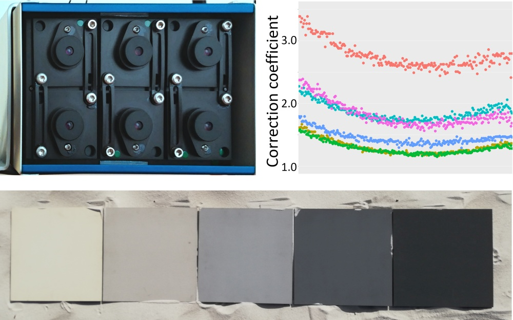
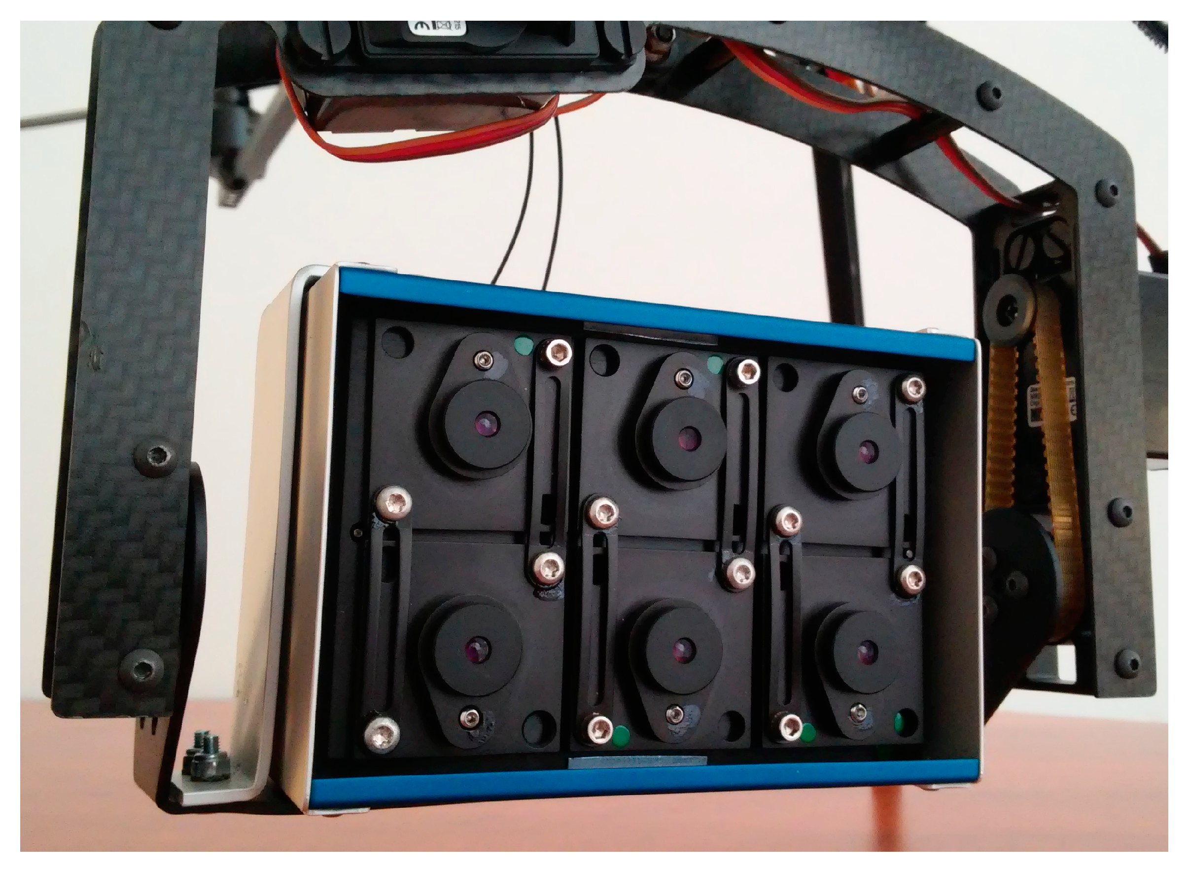
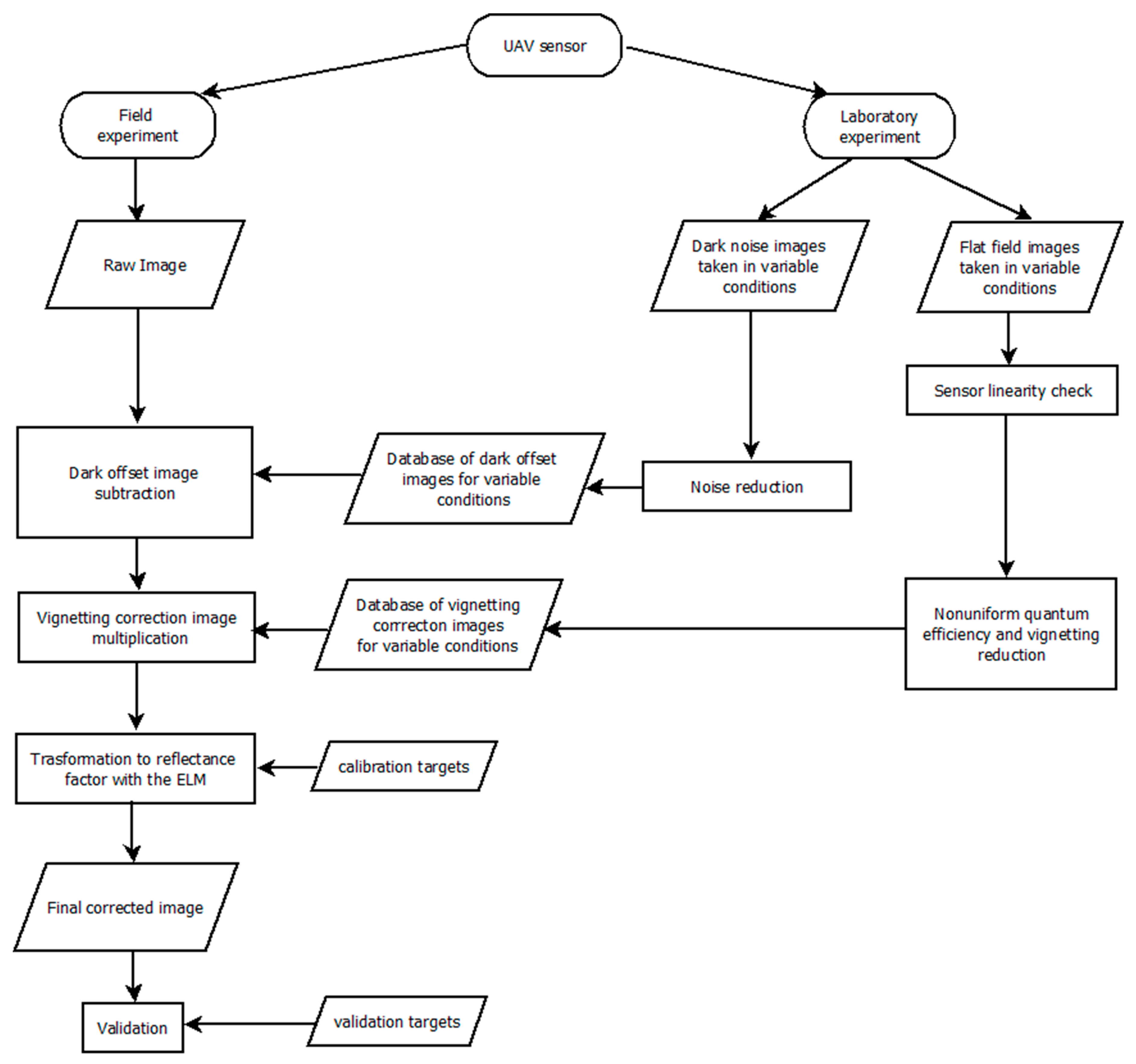
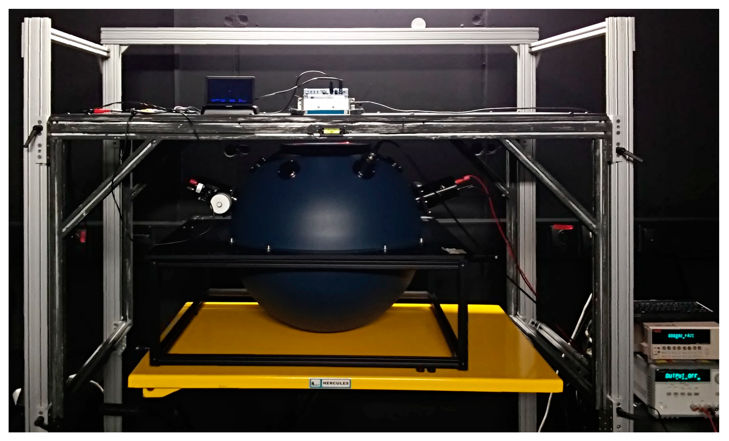
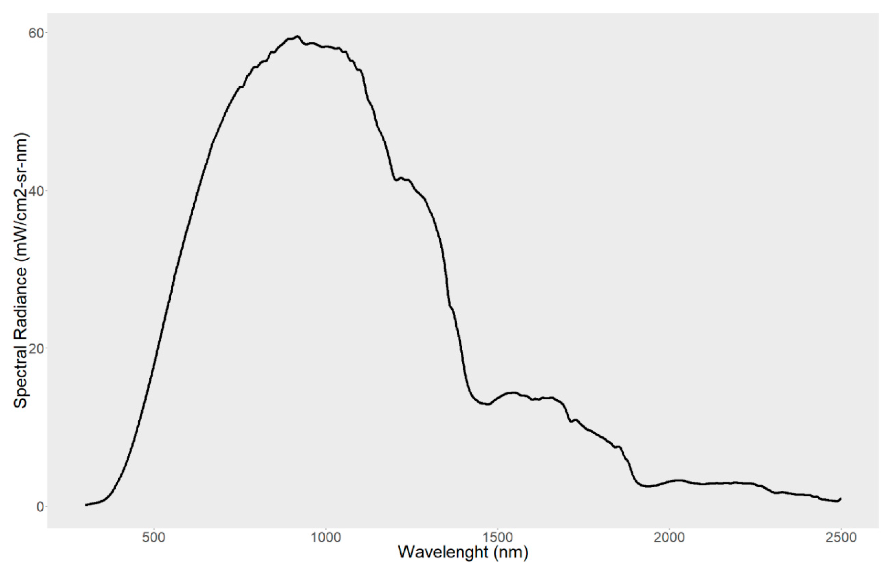
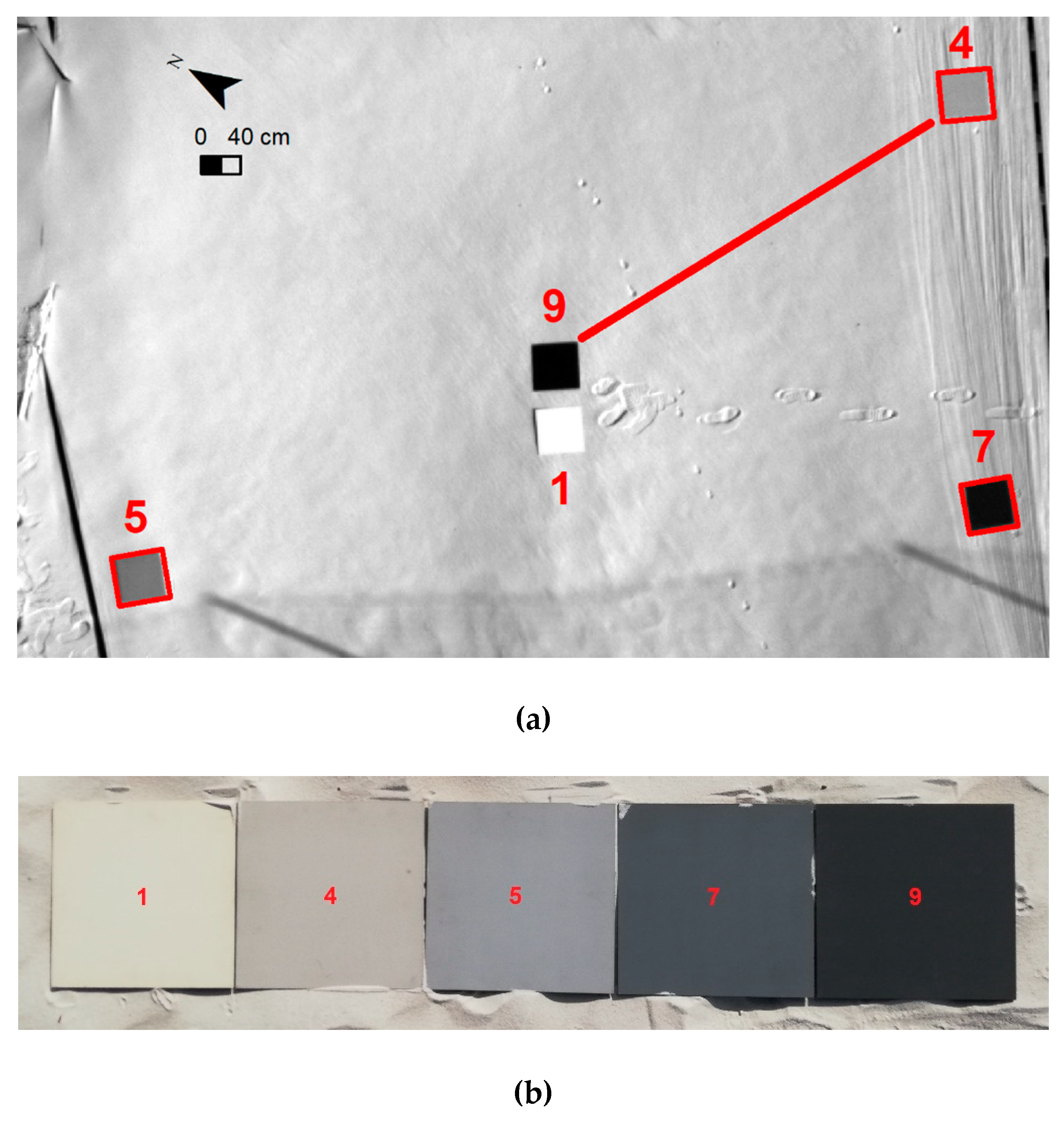
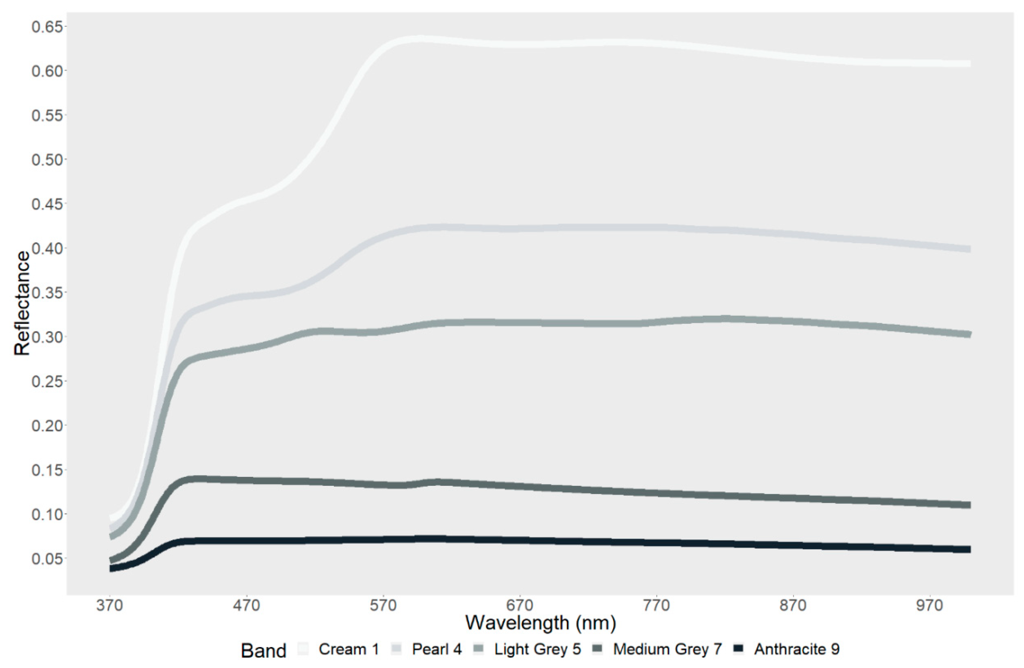
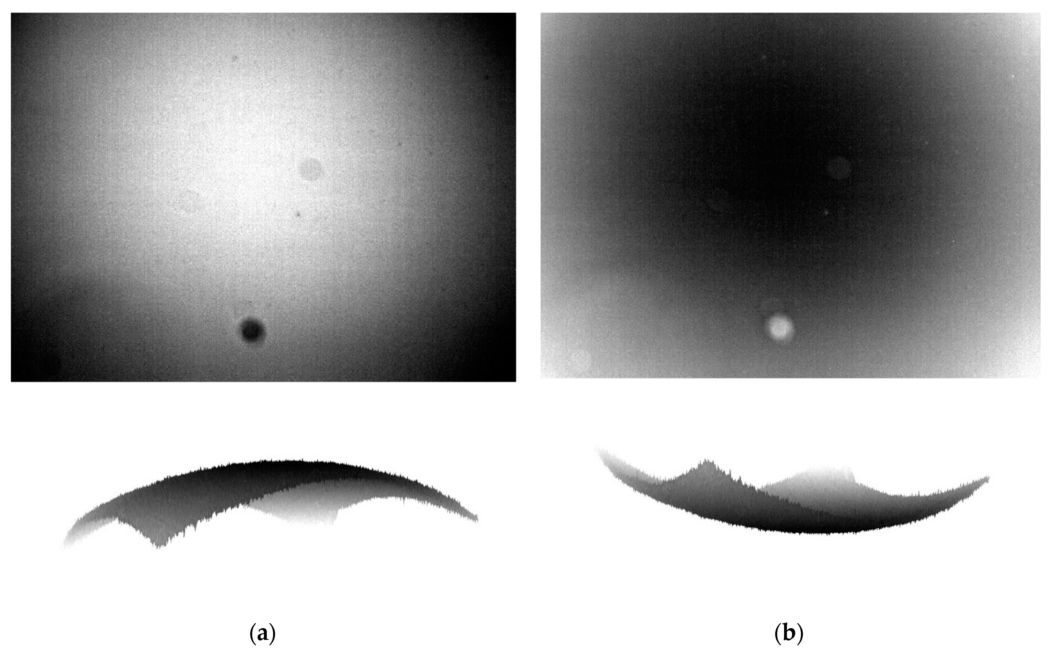
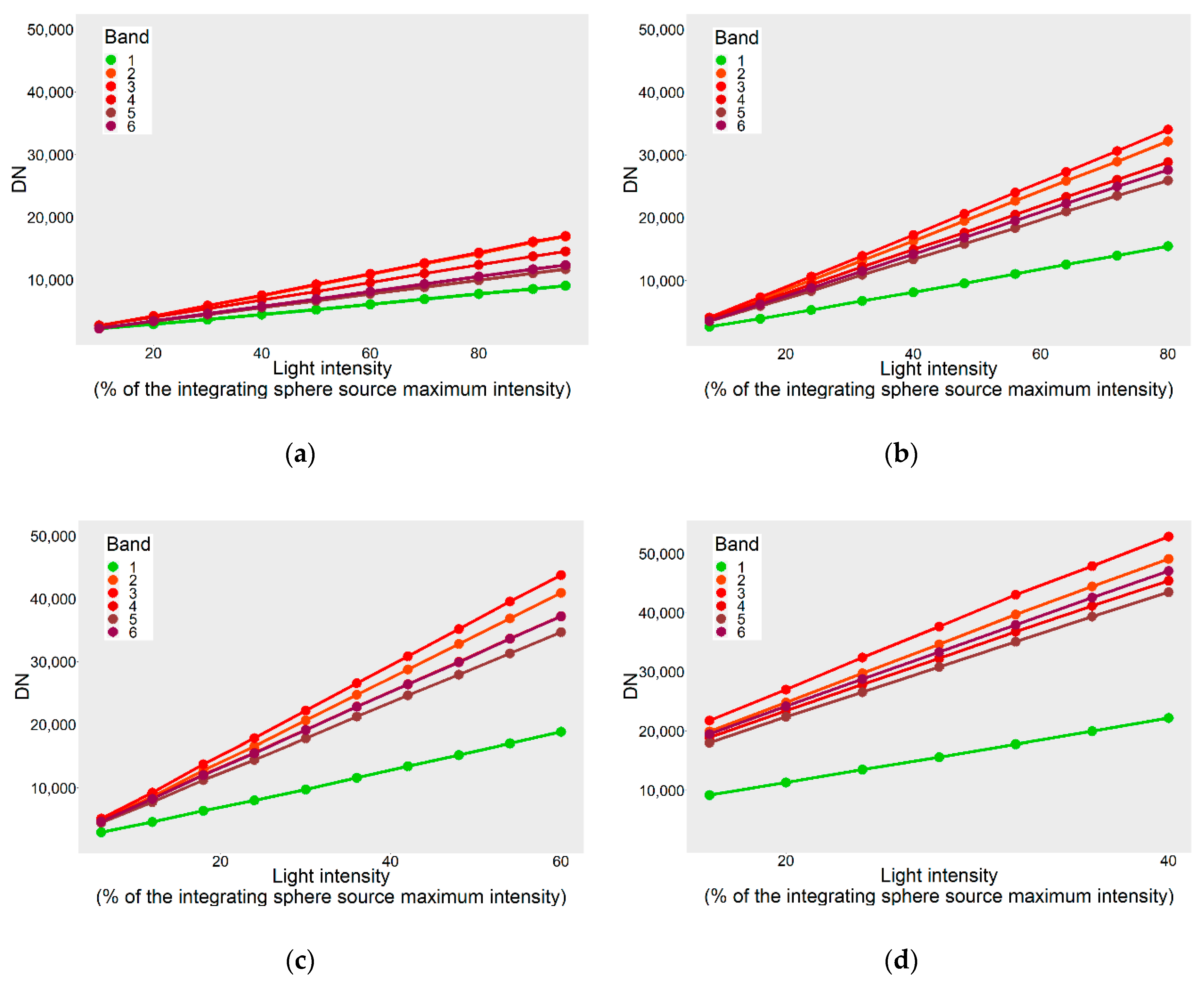
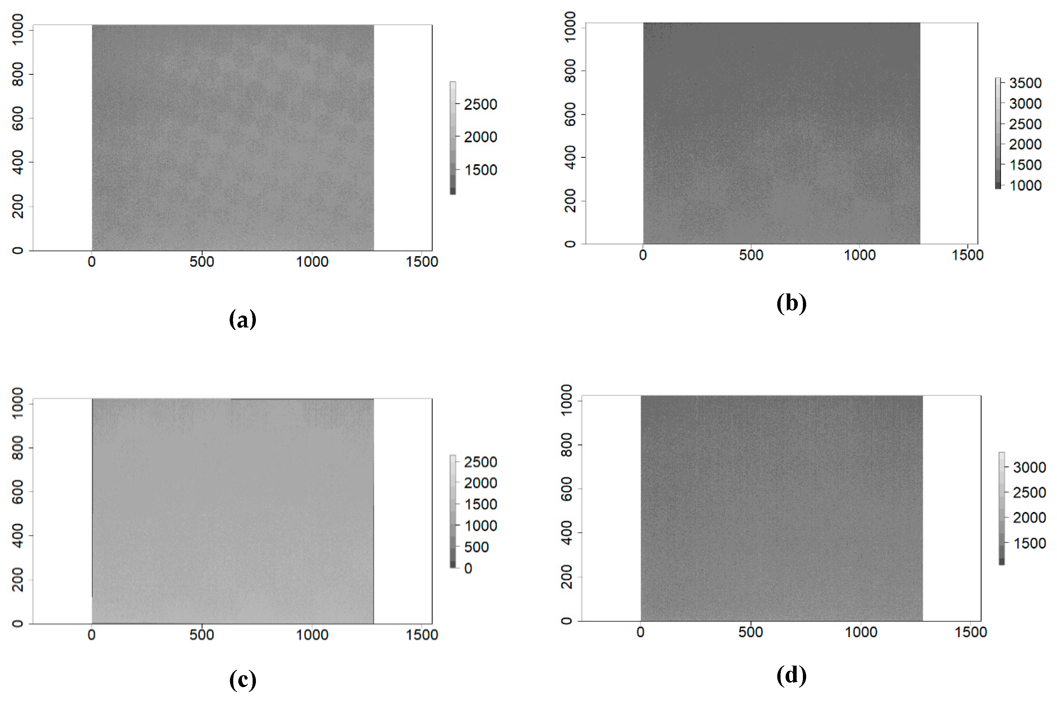
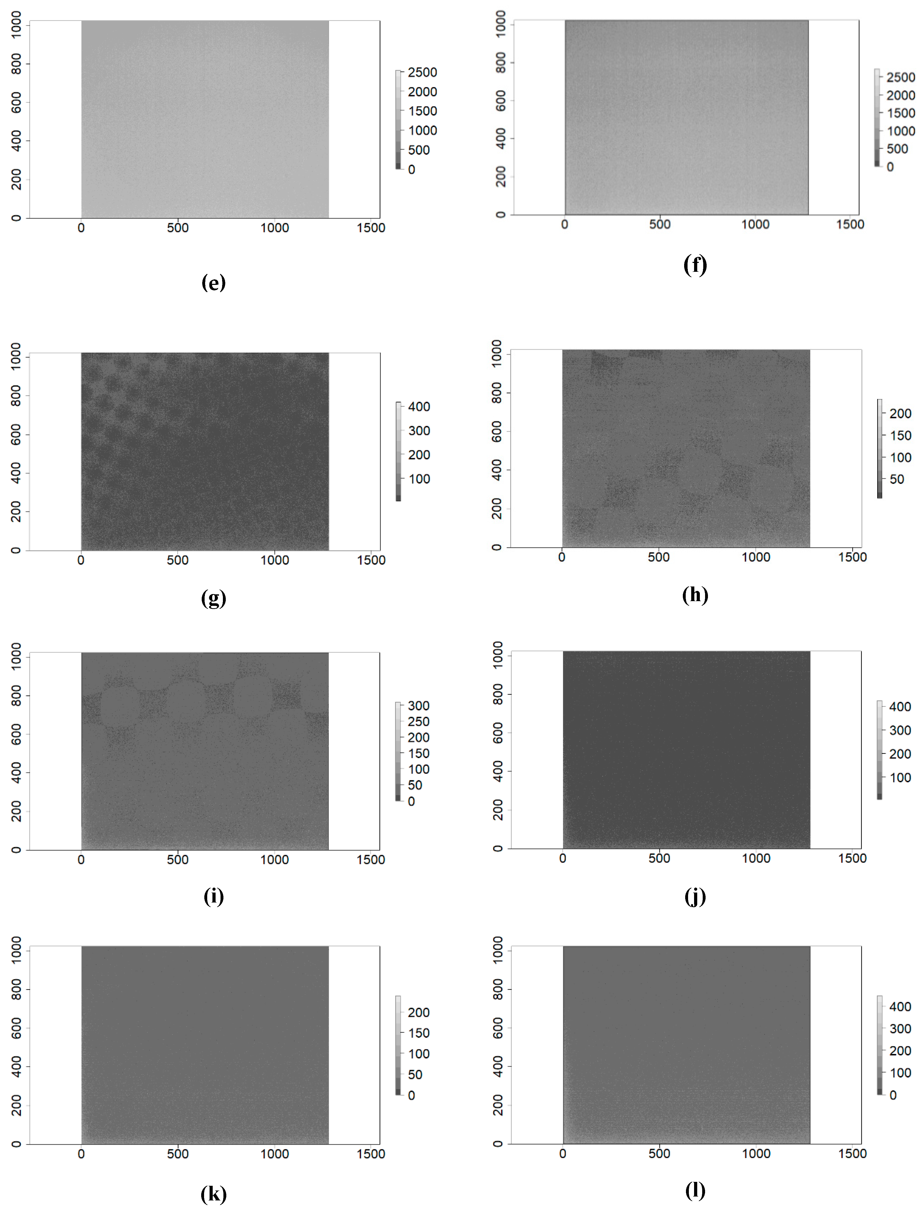
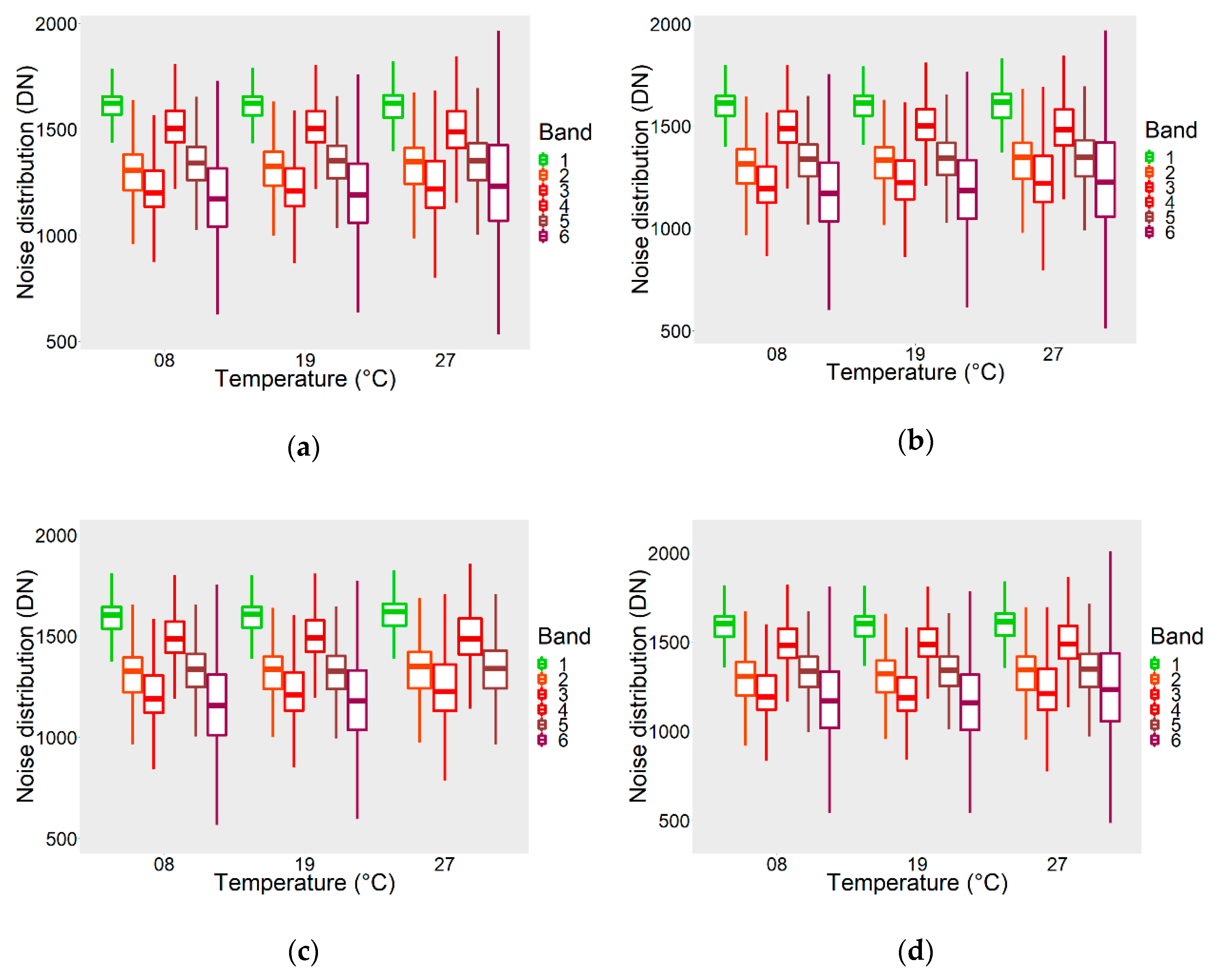
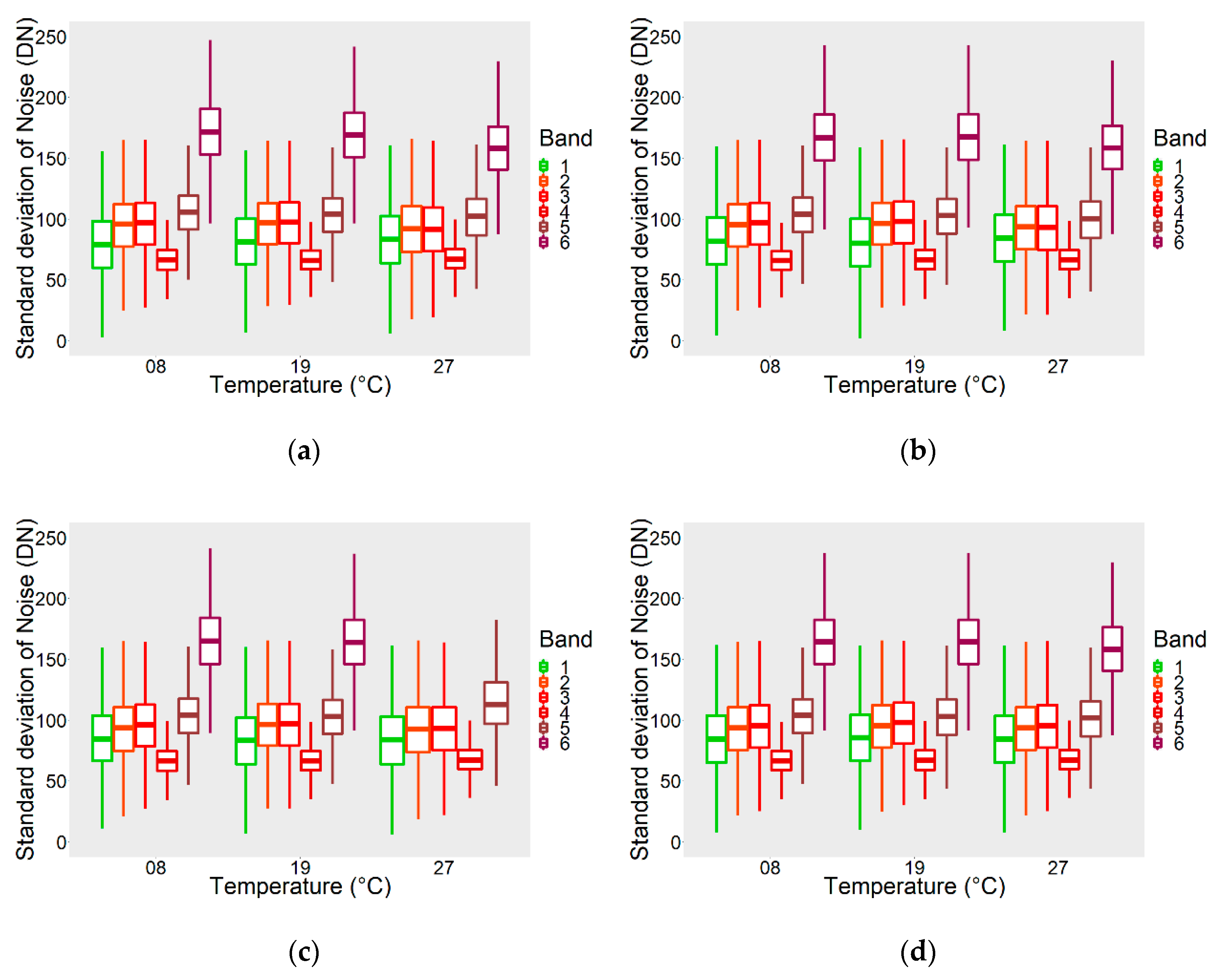
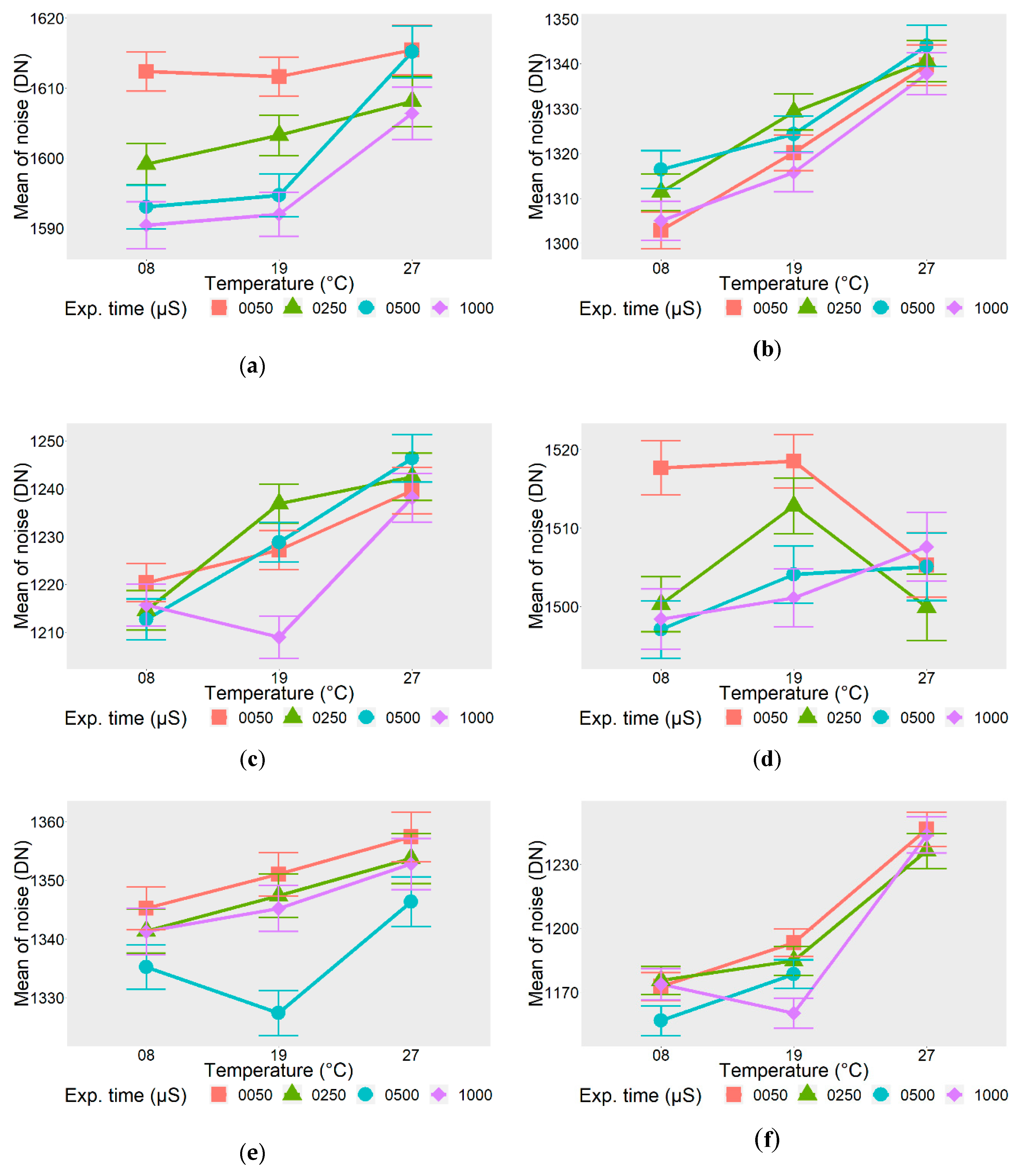
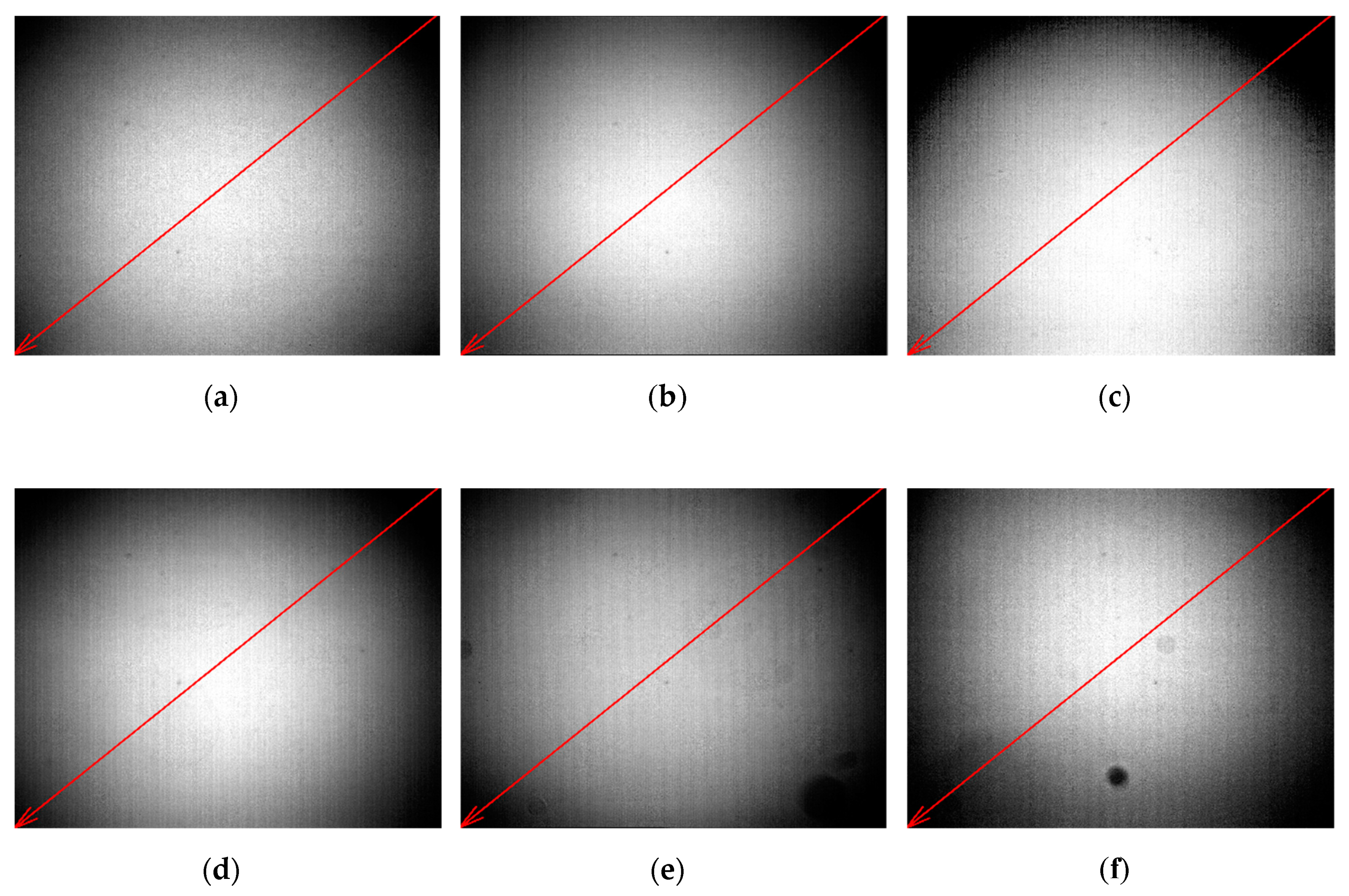
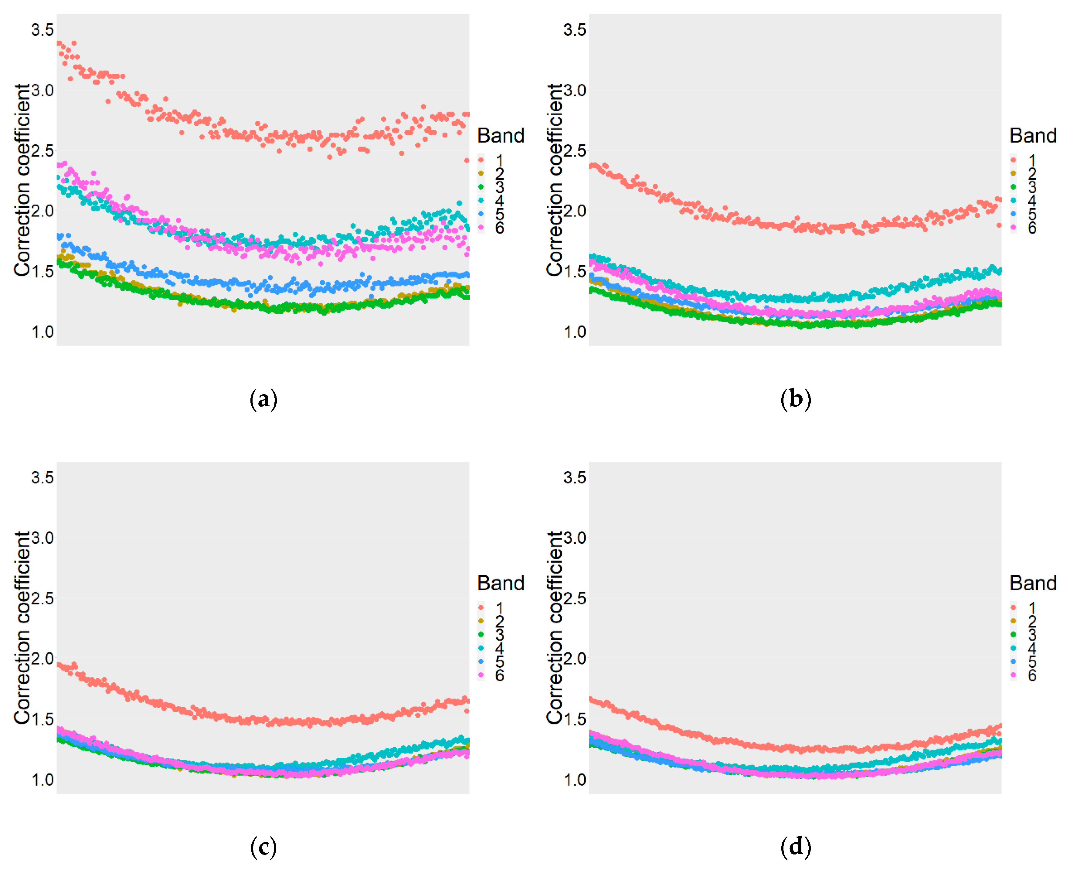
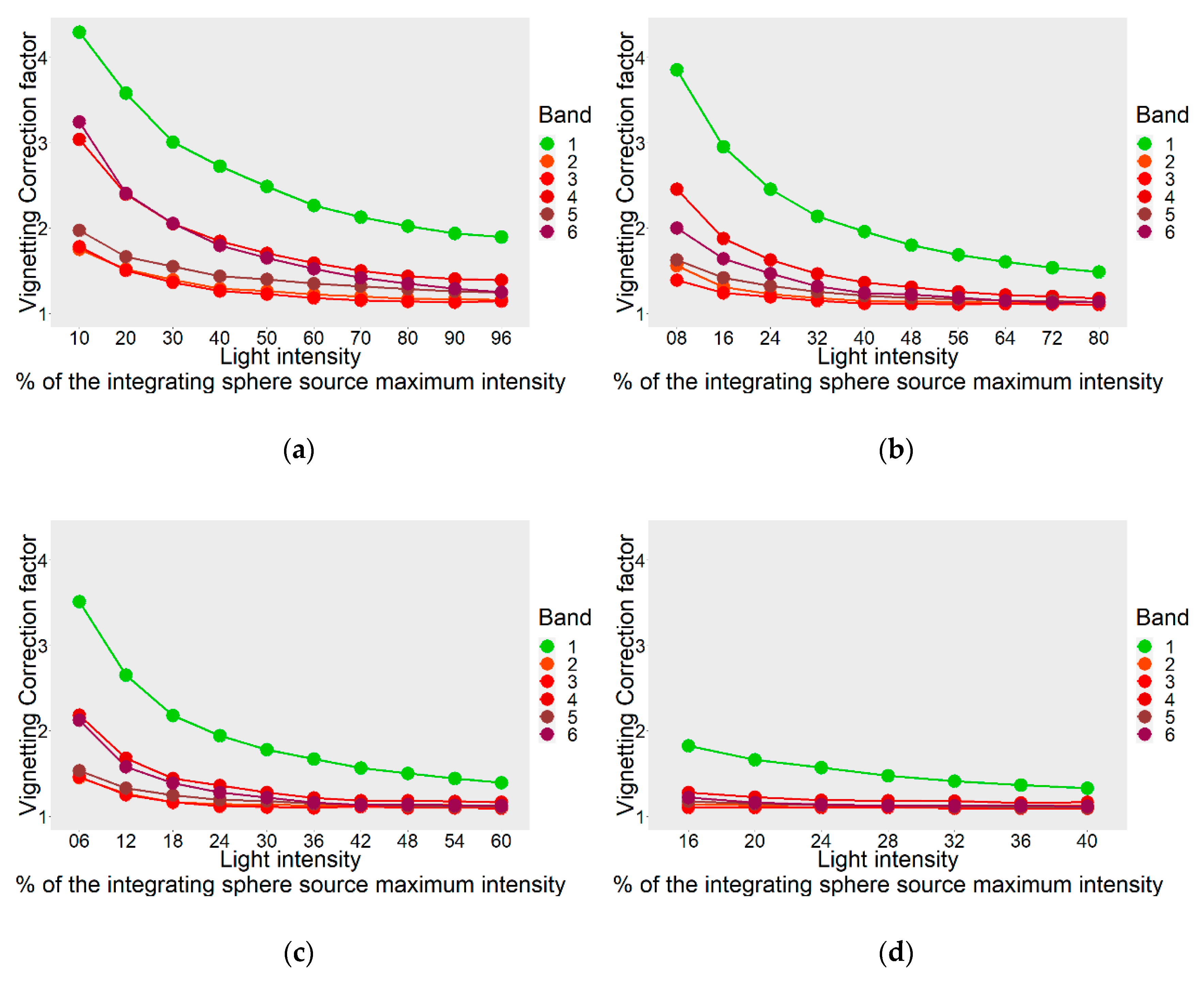
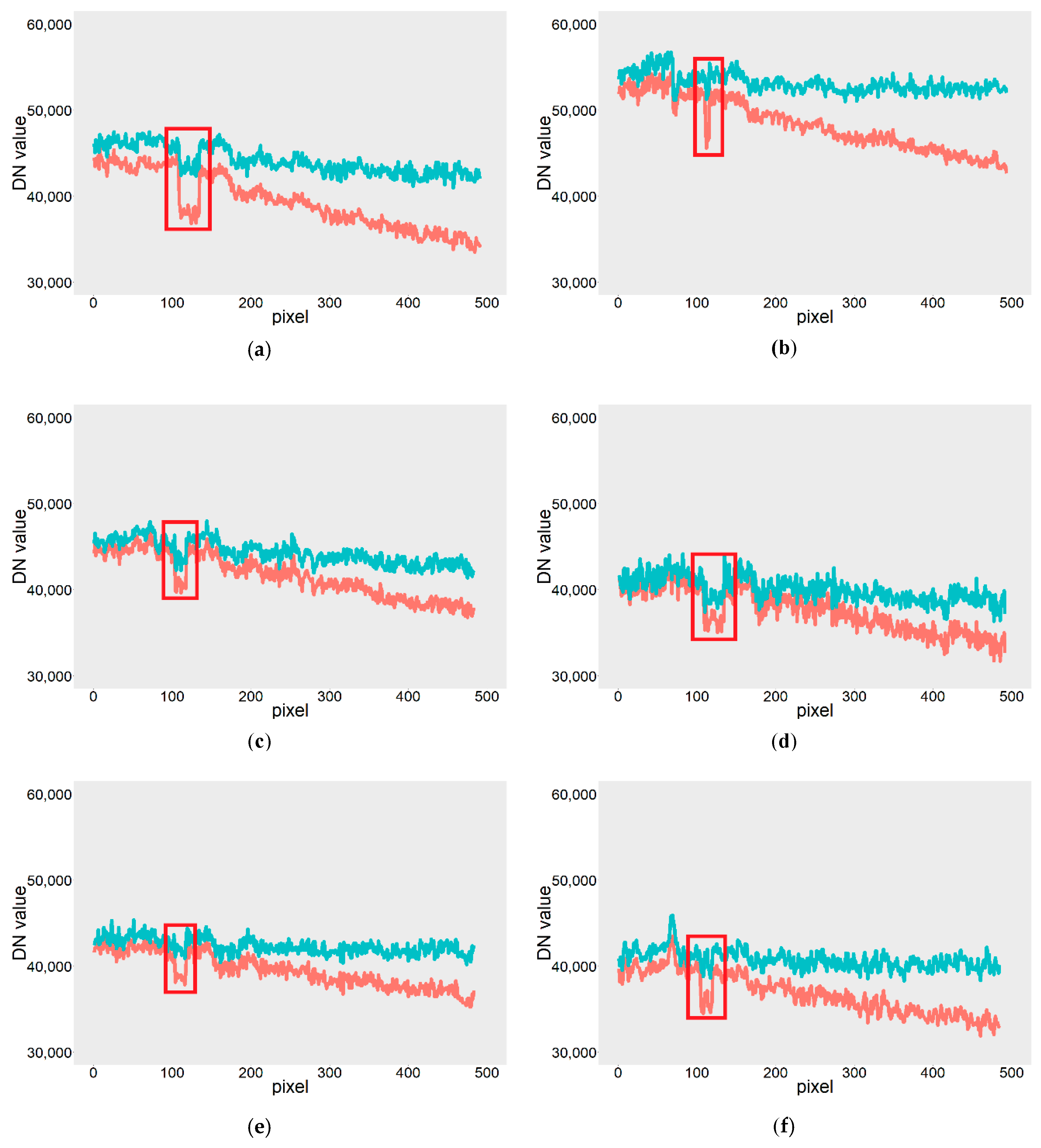
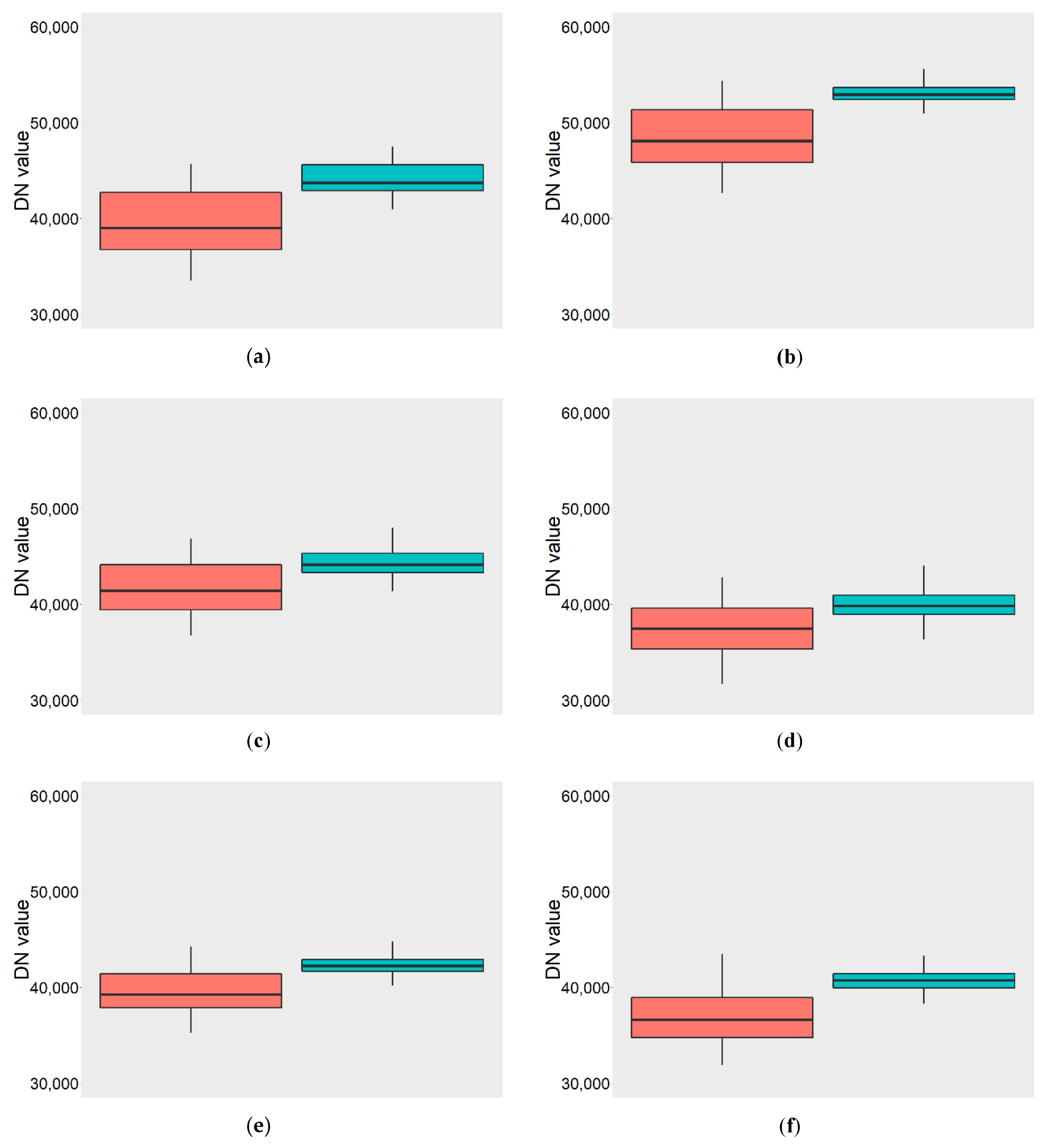
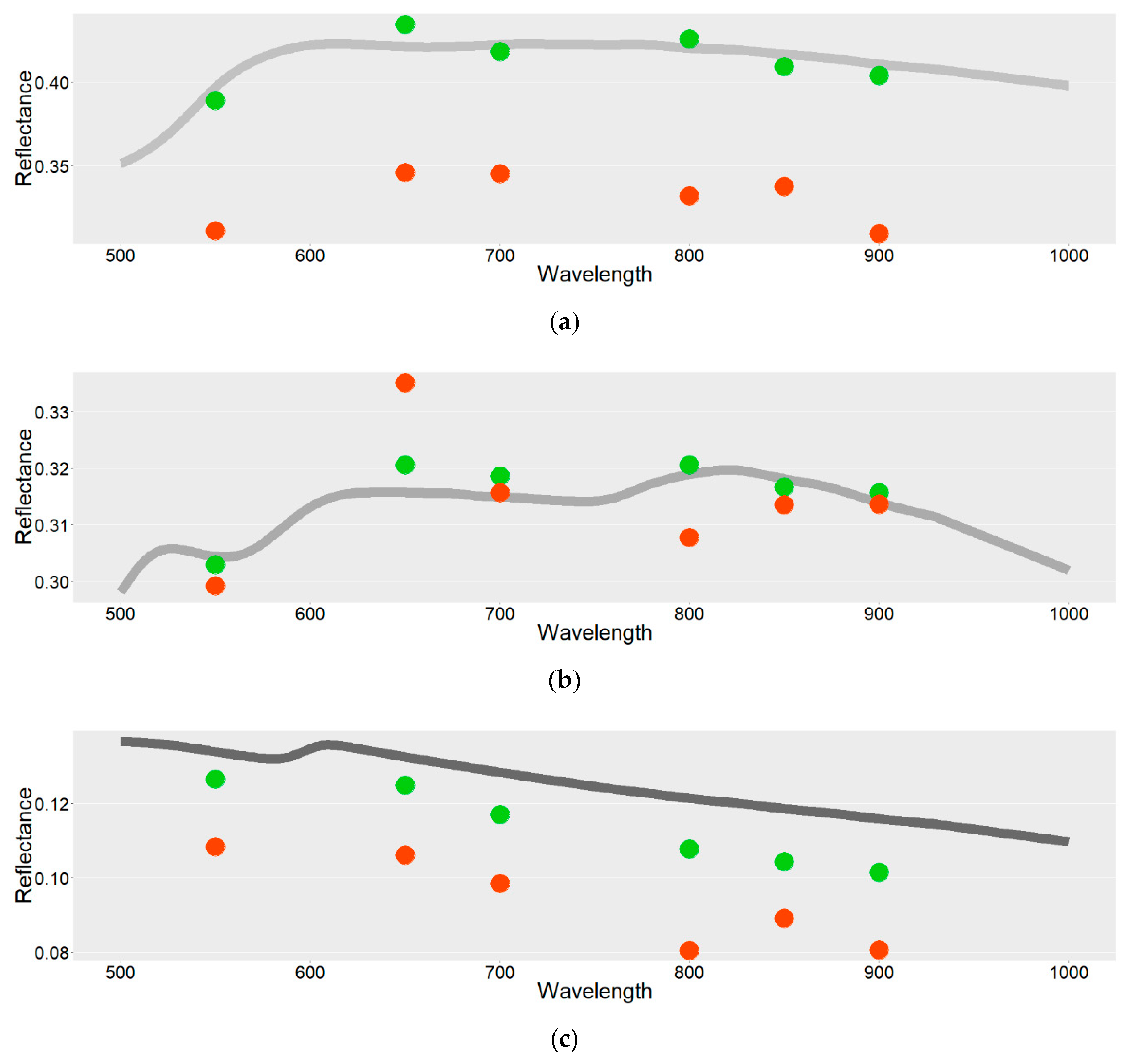
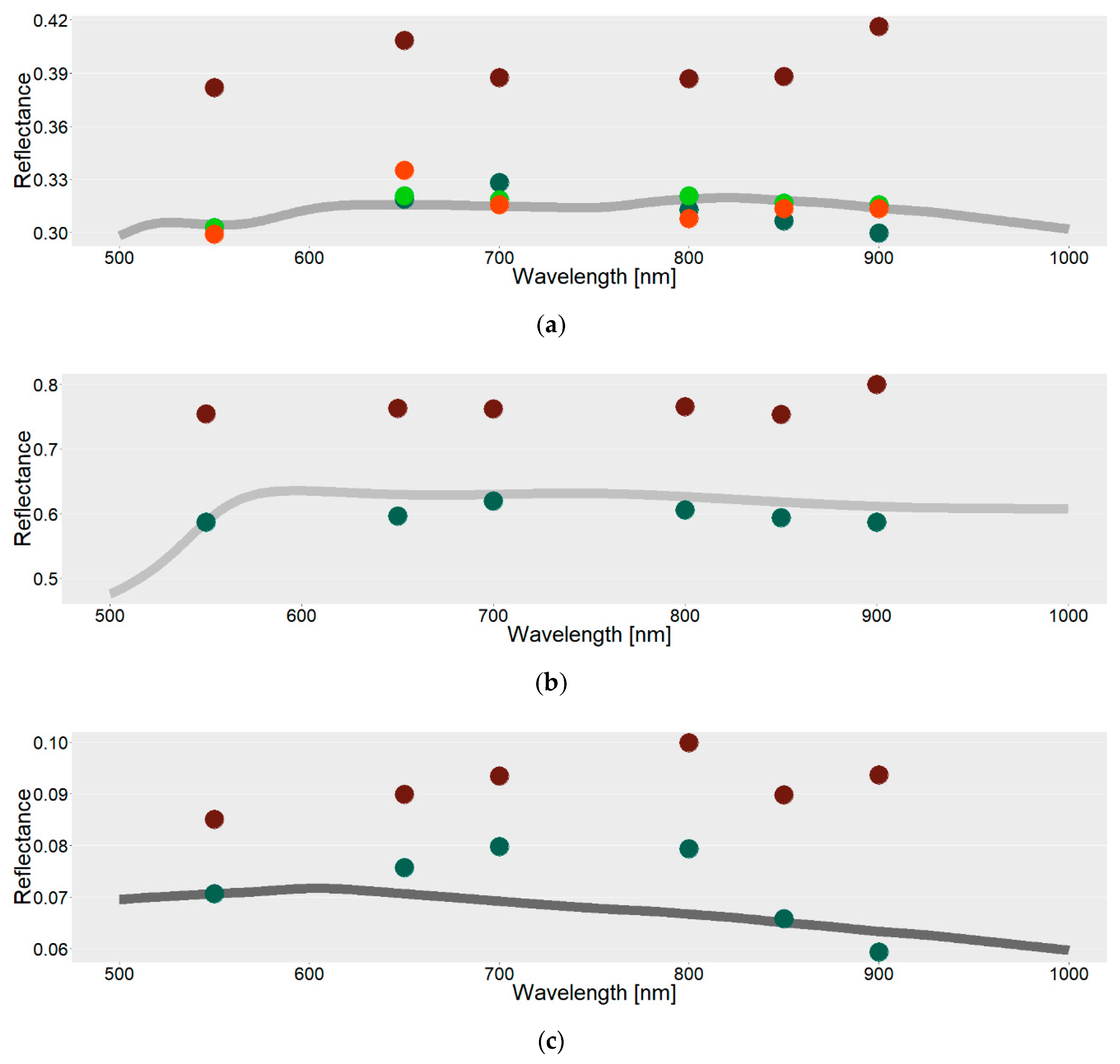
Table 1.
The parameters of Tetracam μ-MCA Snap 6 camera.
| Specification | Description/Value |
|---|---|
| Type | µMCA 6 Snap, 6 identical global shutter sensors, changeable bandpass filters |
| Sensor | 1.3 mega-pixel CMOS sensor (1280 × 1024 pixels) |
| Sensitivity | ~450 nm to ~1000 nm |
| Pixel Size | 4.8 microns |
| Focal length | 9.6 mm fixed lens |
| Aperture | f/3.2 |
| Horizontal Angle of View | 38.26° |
| Vertical Angle of View | 30.97° |
| Default Depth of Field | ~2 m to infinity |
| Bands | B1: 550 nm (FWHM 20 nm) |
| B2: 650 nm (FWHM 20 nm) | |
| B3: 700 nm (FWHM 20 nm) | |
| B4: 800 nm (FWHM 20 nm) | |
| B5: 900 nm (FWHM 20 nm) | |
| B6: 950 nm (FWHM 20 nm) |
Table 2.
The design of the experiment investigating the sensor linearity. Light intensity is given as a percentage of the integrating sphere source maximum light intensity. The maximum power of the source is 1 mA. Only the first 7 levels of light intensity were used in the 1000 μS experiment to avoid the image saturation.
| Exposure Time (µS) | Light Intensity % |
|---|---|
| 50 | 10, 20, 30, 40, 50, 60, 70, 80, 90, 96 |
| 250 | 8, 16, 24, 32, 40, 48, 56, 64, 72, 80 |
| 500 | 6, 12, 18, 24, 30, 36, 42, 48, 54, 60 |
| 1000 | 16, 20, 24, 28, 32, 36, 40 |
Table 3.
The factorial design of experiment studying the effects of the ambient temperature and exposure time on the amount of image noise as a main user-controllable sources of noise in laboratory.
Table 3.
The factorial design of experiment studying the effects of the ambient temperature and exposure time on the amount of image noise as a main user-controllable sources of noise in laboratory.
| Temperature (°C) | Exposure Time (µS) |
|---|---|
| 8 | 50 |
| 250 | |
| 500 | |
| 1000 | |
| 19 | 50 |
| 250 | |
| 500 | |
| 1000 | |
| 27 | 50 |
| 250 | |
| 500 | |
| 1000 |
Table 4.
The repeated measures analysis of variance (ANOVA) table of ambient temperature (temp) and exposure time (exptime) upon image noise. The column statistics shows degrees of freedom after Greenhouse-Geisser correction. The F value column represents the values of test statistics for each model term, p value represents the test significance for this term.
| Band | Expression | Statistics | F-Value | p-Value |
|---|---|---|---|---|
| B1 | temp | F(1.35, 1348.41) | 57.57 | <0.001 |
| exptime | F(2.69, 2682.73 | 106.70 | <0.001 | |
| temp:exptime | F(5.50, 5808.43) | 21.97 | <0.001 | |
| B2 | temp | F(1.66, 1658.68) | 327.60 | <0.001 |
| exptime | F(2.93, 2922.19) | 41.31 | <0.001 | |
| temp:exptime | F(5.91, 5906.79) | 8.54 | <0.001 | |
| B3 | temp | F(1.34, 1697.68) | 163.14 | <0.001 |
| exptime | F(2.74, 2741.60) | 43.91 | <0.001 | |
| temp:exptime | F(5.87, 5868.6) | 38.29 | <0.001 | |
| B4 | temp | F(2, 1998) | 44.46 | <0.001 |
| exptime | F(3, 2997) | 150.28 | <0.001 | |
| temp:exptime | F(6, 5994) | 60.26 | <0.001 | |
| B5 | temp | F(1.67, 1676.18) | 53.26 | <0.001 |
| exptime | F(2.89, 2888.67) | 80.76 | <0.001 | |
| temp:exptime | F(5.85, 5842.95) | 10.28 | <0.001 | |
| B6 | temp | F(1.47, 1472.17) | 559.63 | <0.001 |
| exptime | F(1.95, 1949.77) | 29.87 | <0.001 | |
| temp:exptime | F(3.91, 3905,11) | 37.38 | <0.001 |
Table 5.
The results of Fligner-Killeen scale test. V means variation of samples extracted from original raw image and fully corrected image.
Table 5.
The results of Fligner-Killeen scale test. V means variation of samples extracted from original raw image and fully corrected image.
| Band | Null Hypotheses | Z-Statistics | p-Value |
|---|---|---|---|
| 1 | 14.347 | <0.001 | |
| 2 | 18.179 | <0.001 | |
| 3 | 13.656 | <0.001 | |
| 4 | 12.889 | <0.001 | |
| 5 | 14.641 | <0.001 | |
| 6 | 15.601 | <0.001 |
Table 6.
The normalized root mean square errors of reflectance values comparing reference spectral curve of verification targets with reflectance values extracted from raw and fully corrected image. The normalization was performed by dividing the RMSE by interquartile range. The values are expressed as percentage.
| Wavelength | RAW 4 | Calibrated 4 | RAW 5 | Calibrated 5 | RAW 7 | Calibrated 7 |
|---|---|---|---|---|---|---|
| 550 | 17.60 | 1.40 | 0.94 | 0.69 | 3.29 | 1.73 |
| 650 | 13.86 | 2.10 | 2.38 | 0.82 | 5.65 | 1.15 |
| 700 | 13.30 | 0.91 | 0.87 | 0.94 | 7.15 | 0.24 |
| 800 | 8.56 | 0.54 | 1.06 | 0.72 | 4.44 | 0.62 |
| 850 | 9.80 | 1.07 | 0.80 | 0.77 | 2.52 | 0.95 |
| 900 | 11.63 | 0.70 | 0.91 | 0.73 | 3.08 | 0.53 |
© 2019 by the authors. Licensee MDPI, Basel, Switzerland. This article is an open access article distributed under the terms and conditions of the Creative Commons Attribution (CC BY) license (http://creativecommons.org/licenses/by/4.0/).
Share and Cite
MDPI and ACS Style
Minařík, R.; Langhammer, J.; Hanuš, J. Radiometric and Atmospheric Corrections of Multispectral μMCA Camera for UAV Spectroscopy. Remote Sens. 2019, 11, 2428. https://0-doi-org.brum.beds.ac.uk/10.3390/rs11202428
AMA Style
Minařík R, Langhammer J, Hanuš J. Radiometric and Atmospheric Corrections of Multispectral μMCA Camera for UAV Spectroscopy. Remote Sensing. 2019; 11(20):2428. https://0-doi-org.brum.beds.ac.uk/10.3390/rs11202428
Chicago/Turabian StyleMinařík, Robert, Jakub Langhammer, and Jan Hanuš. 2019. "Radiometric and Atmospheric Corrections of Multispectral μMCA Camera for UAV Spectroscopy" Remote Sensing 11, no. 20: 2428. https://0-doi-org.brum.beds.ac.uk/10.3390/rs11202428
Note that from the first issue of 2016, this journal uses article numbers instead of page numbers. See further details here.