Upper Ocean Response to Two Sequential Tropical Cyclones over the Northwestern Pacific Ocean


1
College of Oceanography, Hohai University, Nanjing 210098, China
2
State Key Laboratory of Satellite Ocean Environment Dynamics, Second Institute of Oceanography, Ministry of Natural Resources, Hangzhou 310012, China
3
Key Laboratory of Marine Environment and Ecology, Ocean University of China, Qingdao 266100, China
4
Qingdao National Laboratory for Marine Science and Technology, Qingdao 266100, China
*
Author to whom correspondence should be addressed.
Remote Sens. 2019, 11(20), 2431; https://0-doi-org.brum.beds.ac.uk/10.3390/rs11202431
Submission received: 28 August 2019
/
Revised: 7 October 2019
/
Accepted: 18 October 2019
/
Published: 19 October 2019
(This article belongs to the Special Issue Tropical Cyclones Remote Sensing and Data Assimilation)
Abstract
:The upper ocean thermodynamic and biological responses to two sequential tropical cyclones (TCs) over the Northwestern Pacific Ocean were investigated using multi-satellite datasets, in situ observations and numerical model outputs. During Kalmaegi and Fung-Wong, three distinct cold patches were observed at sea surface. The locations of these cold patches are highly correlated with relatively shallower depth of the 26 °C isotherm and mixed layer depth (MLD) and lower upper ocean heat content. The enhancement of surface chlorophyll a (chl-a) concentration was detected in these three regions as well, mainly due to the TC-induced mixing and upwelling as well as the terrestrial runoff. Moreover, the pre-existing ocean cyclonic eddy (CE) has been found to significantly modulate the magnitude of surface cooling and chl-a increase. With the deepening of the MLD on the right side of TCs, the temperature of the mixed layer decreased and the salinity increased. The sequential TCs had superimposed effects on the upper ocean response. The possible causes of sudden track change in sequential TCs scenario were also explored. Both atmospheric and oceanic conditions play noticeable roles in abrupt northward turning of the subsequent TC Fung-Wong.
1. Introduction
Tropical cyclones (TCs), which are among the most devastating natural disasters, pose significant threat on the lives and property of global coastal regions [1]. During the passage of a TC, the strong wind stress could typically produce intense oceanic entrainment and upwelling [2,3,4], which leads to physical and biological responses of the upper ocean. Sea surface temperature (SST) decrease, the most striking phenomenon, is usually observed in the range of 1–9 °C with stronger cooling to the right side of a TC’s track [5,6,7,8,9]. The sea surface cooling has a negative feedback to a TC by suppressing the TC development in turn [10]. Furthermore, the SST decrease would have an impact on the subsequent TCs if they pass by these cold wakes coincidentally [11]. The distribution of phytoplankton biomass, as is measured by chlorophyll a (chl-a) concentration, is also influenced by TCs. Previous studies have found that the surface chl-a concentration would be largely increased after TCs, with estimated maximum contribution of 20–30% for the annual new production in the South China Sea (SCS) [12,13]. It is well recognized that the magnitude and spatial distribution of SST decrease and chl-a enhancement mainly depend on the intensity and translation speed of TCs and the background ocean environments, such as the mixed layer depth (MLD) and mesoscale eddies, as well as topography [2,13,14,15,16]. Owing to the complex pre-TC conditions of different regions, the responses of the upper ocean in these regions are well worth studying in detail. Although the upper ocean response to a single TC has been commonly focused on [6,7,8,9,17,18,19,20], inadequate attention is paid to how sequential TCs affect the upper ocean from both physical and biological aspects.
The mesoscale cyclonic eddy (CE), as one of the main pre-TC ocean features, plays an important role in the upper ocean response to TCs [7,8,21,22,23]. CEs with negative sea surface height anomaly (SSHA) and cold water in the core region provide a relatively unstable thermodynamic structure that help elevate cold and nutrient-rich water below easily [7,8,21]. Conversely, CEs might be influenced by individual TC in many ways [23,24]. However, the interaction between sequential TCs and CEs still remains unclear.
It seems that more intense TCs happen annually under the background of warming climate [25]. Nevertheless, the current level of TC forecast does lay behind the urgent needs of disaster prevention and mitigation [26]. Particularly, when two or more TCs exist simultaneously in the same region, it becomes much more difficult to forecast their tracks [27,28]. Previous studies suggested both atmospheric and oceanic factors could affect the forecast accuracy of the TC by influencing its motion and intensity, such as western North Pacific subtropical high (WNPSH), the environmental flow, SST and upper ocean heat content (UOHC) [29,30,31,32,33]. However, how these factors contribute to the sudden track change in sequential TCs scenario has been seldom systematically investigated. Thus, it is essential to comprehensively understand the possible causes under complex atmospheric and ocean environments.
This study aims to explore the thermodynamic and biological responses of the upper ocean to two sequential TCs over the Northwestern Pacific Ocean (NWP) in 2014 and reveal the possible causes leading to the sudden track change of the subsequent TC in this scenario. A brief description of the datasets and methods is presented in Section 2. Section 3 gives the results and discussion in detail. Finally, the conclusions are made in Section 4.
2. Data and Methods
2.1. Data
2.1.1. TC Best Track Data
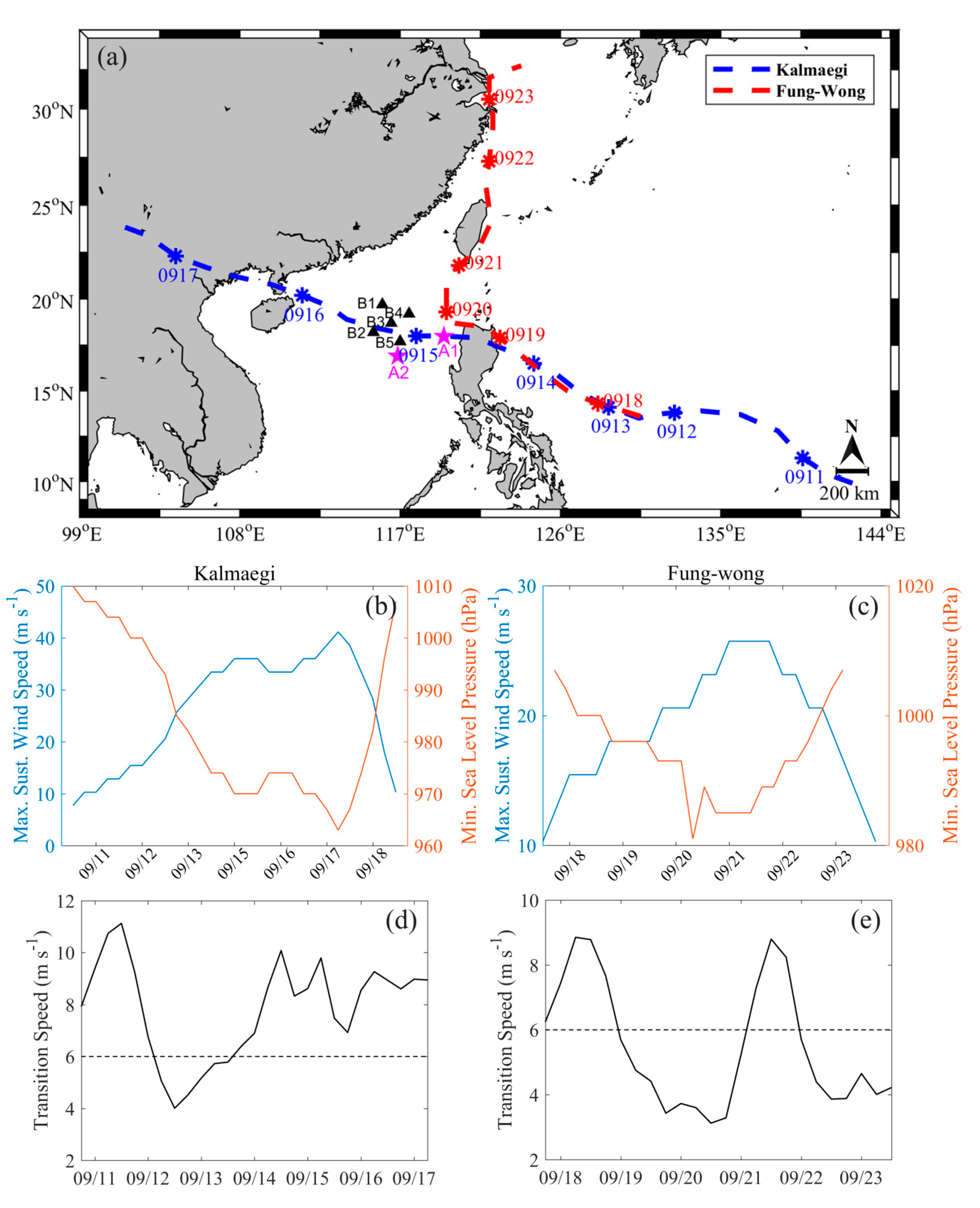
The TC information, including the time (UTC), center location, the maximum sustained wind speed (MSW) and minimum sea surface pressure every 6 hours, is obtained from Joint Typhoon Warning Center (JTWC, http://www.usno.navy.mil/NOOC/nmfc-ph/RSS/jtwc/best_tracks). The best track dataset is suggested to be more dynamically consistent than some other datasets [34]. The tracks and intensities of Kalmaegi and Fung-Wong in September 2014 are shown in Figure 1a–c. Based on the time series of center locations, the translation speeds of the two TCs are calculated (Figure 1d,e). TC Kalmaegi formed on September 10 in the Tropical Pacific. It went straight northwest, crossed the South China Sea, and finally made landfall in Hainan Province on September 16. The largest MSW reached 80 kt (i.e., 41 m s−1) as a Category 1 TC.
After one week, Tropical Storm Fung-Wong formed in the area where Kalmaegi passed by and then followed the Kalmaegi’s track to the northwest. While until September 20, a sudden turning occurred over the Luzon Strait. Afterward it moved to the north and landed in Zhejiang Province on September 22. It reached its peak MSW at 50 kt (26 m s−1) on September 21.
2.1.2. Satellite Observations
The daily SST product used in this study is Microwave and Infrared OI SST (MW-IR OISST) from the Remote Sensing Systems (http://www.remss.com/) with a spatial resolution of 9 km × 9 km. It combines the through-cloud capability of the microwave OI SST product [35] with the high spatial resolution of the infrared SST by using Optimum Interpolation method [36].
The daily SSHA dataset, provided by Archiving, Validation and Interpretation of Satellite Data in Oceanography (AVISO) has a spatial resolution of 0.25° × 0.25°. The altimeter products are produced and distributed by the Copernicus Marine and Environment Monitoring Service (CMEMS, http://marine.Copernicus.eu/). Closed contours of negative SSHA are normally corresponding to mesoscale cyclonic eddies (CEs) with cold water in the core region [8].
Because the daily chl-a concentration dataset includes plenty of data gaps caused by severe cloud contamination, we use the 8-day averaged data to study the biological response of the upper ocean to the sequential TCs. Previous studies pointed out that phytoplankton growth, which attributes to chl-a enhancement under the influence of a TC, needs a delay of several days (∼5 days) to reach its peak [21]. The accurate days for chl-a concentration to rise to its maximum remains unclear [22]. The merged 8-day chl-a concentration data, with a spatial resolution of 4 km × 4 km, produced and distributed by the GlobColour Project (http://hermes.acri.fr/) are satisfied with the basic research requirements [22]. The GlobColour data were developed, validated, and distributed by ACRI-ST, France.
The daily ocean surface winds on a global 0.25° grid derived from the Blended Sea Winds dataset are acquired from the National Oceanic and Atmospheric Administration’s (NOAA’s) National Climatic Data Center, via their website (http://http://www.ncdc.noaa.gov/oa/rsad/air-sea/ seawinds.html). The gridded wind speeds were created from the blending observations of multiple satellites [37].
2.1.3. In Situ Measurements
Temperature and salinity profiles used to investigate the thermal responses are obtained from Argo observations and a cross-shaped observational array in the SCS deployed by the Second Institute of Oceanography, Ministry of Natural Resources of China in 2014. The Argo profiles are provided by the China Argo Real-time Data Center (http://www.argo.org.cn/) and the quality control has been performed [38]. The locations of Argo floats and observational array are shown in Figure 1a. There are two Argo floats located in the area influenced by both Kalmaegi and Fung-Wong. The observational array consists of five moored buoys and four subsurface moorings organized into five stations. Considering the validity of the data and the distance between the stations and two TCs, the data at Stations 4 and 5 are analyzed in this study.
2.1.4. Ocean Numerical Model Outputs
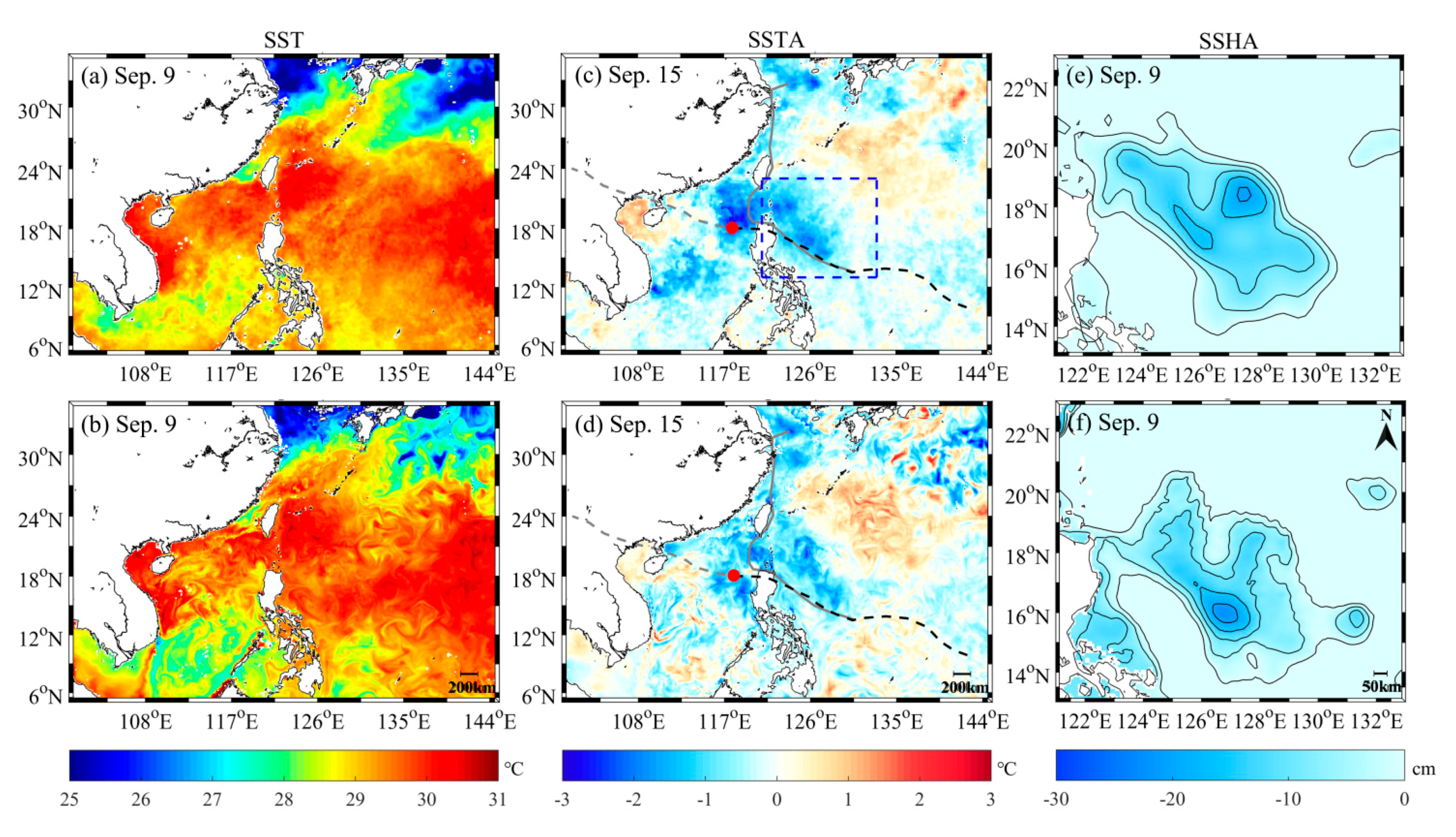
The daily ocean analysis data with a spatial resolution of 0.08° × 0.08° are obtained from the global HYbrid Coordinate Ocean Model (HYCOM) + Navy Coupled Ocean Data Assimilation (NCODA) based ocean prediction system (hereafter called HYCOM, https://www.hycom.org/) [39]. As shown in Figure 2, HYCOM simulations of SST, SST difference (SSTD) during and before Kalmaegi passed by and SSHA are in good agreement with satellite observations. It is clear that the SSHA from HYCOM and AVISO both reveal the same CE region. Therefore, the data can be used for further analysis.
2.1.5. Atmospheric Reanalysis Data
The atmospheric fields are obtained from the National Centers for Environmental Prediction–Department of Energy (NCEP–DOE) AMIP-II reanalysis 2 data, which is from the National Oceanic and Atmospheric Administration (NOAA) Earth System Research Laboratory’s Physical Sciences Division (https://www.esrl.noaa.gov/psd/). The reanalysis data have a spatial resolution of 2.5° × 2.5° on a global grid and 17 pressure levels from 10 to 1000 hPa [40].
2.2. Methods
In this study, SST on September 9 is considered to be the pre-TCs condition. The SSTD, which denotes the SST variation during and before TCs pass by, can be calculated from satellite observations or HYCOM data by subtracting SST during the TCs and that on September 9.
The MLD, defined as the depth where the temperature decreases 0.5 °C compared to that at surface [41], or that was based on density variation according to Equation (1) of Kara et al. (2000) [41], is calculated from temperature sections of Argo profiles, observational array and HYCOM data. The temporal variations of MLDs are similar when we use temperature or density criterion, although the absolute values of the later are a little smaller. Here, the results of MLD calculated by temperature criterion are adopted. Mixed layer temperature (MLT) and mixed layer salinity (MLS) are taken as the average values in the mixed layer.
The UOHC is calculated using HYCOM output of ocean temperature profiles T(z):
where is the seawater density (1024 kg/m3); is the heat capacity (4186 J/kg °C). D26 is the depth of the 26 °C isotherm, which can characterize the relative warm or cold of the upper ocean.
The potential upwelling speed due to TC winds is calculated using the classical Ekman pumping velocity (EPV) formula [4]:
where is the Coriolis parameter. The wind stress can be obtained by the bulk formula [42]:
where is the air density; and are the wind speed and wind vector 10 meters above sea surface, respectively; is the drag coefficient and is calculated using the formula proposed by Oey et al. (2006) [43], which fits the formula at low-to-moderate wind speeds [44] and the results at high wind speeds [45],
3. Results and Discussion
3.1. Thermodynamic Response
3.1.1. Sea Surface Cooling
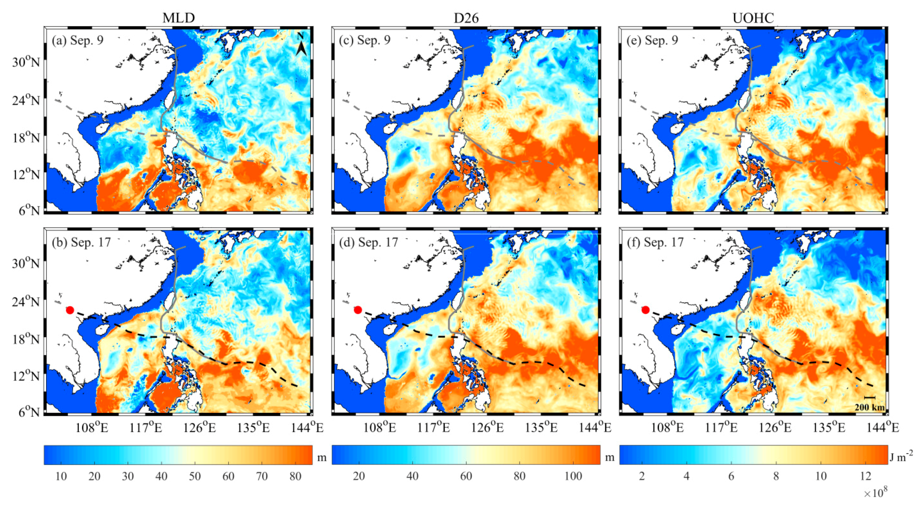
As shown in Figure 3a and Figure 4a,c,e, the background ocean environments on September 9 provided favorable conditions for TC generation, with high SST, relatively deep D26, MLD and high UOHC. The SST in most part of study area was higher than 30 °C. During the passages of both Kalmaegi and Fung-Wong, there was a cool trail along their tracks with rightward bias (Figure 3b–f). In particular, three distinct cold patches were detected, which were marked with black, gray and red box and correspondingly labeled as R1, R2, R3 in Figure 3, respectively.
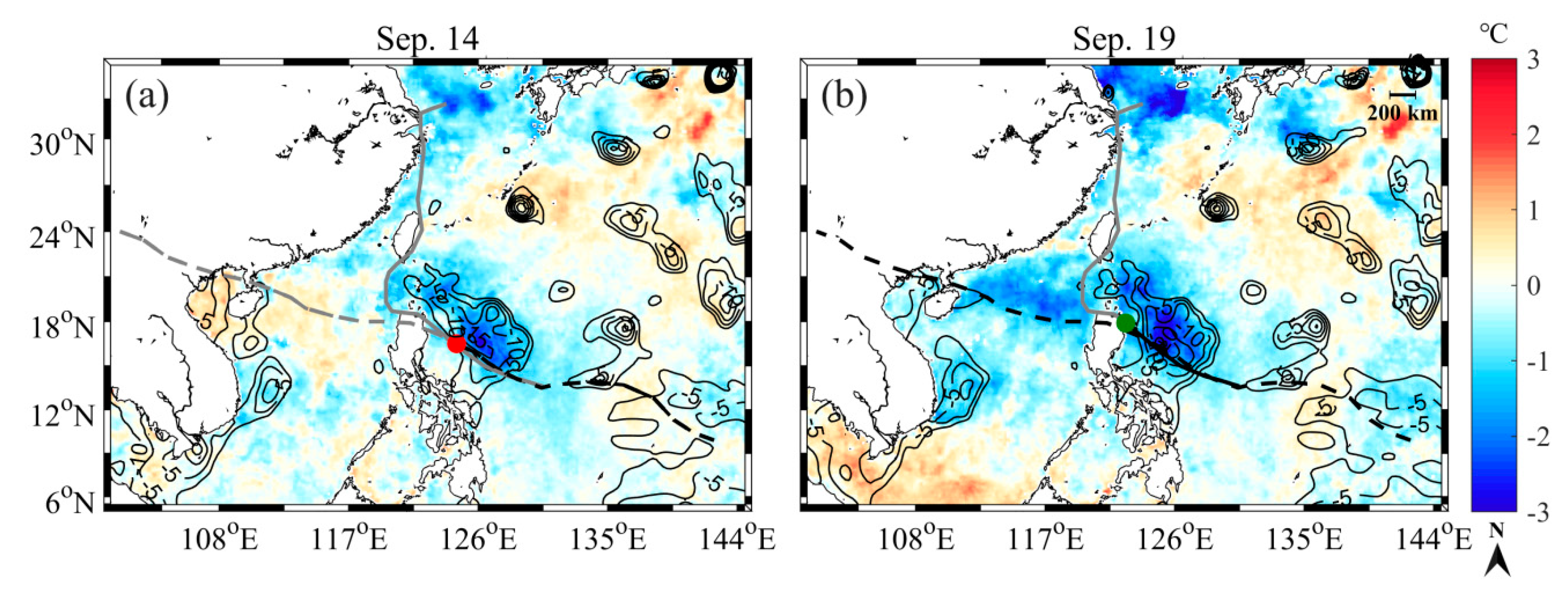
In region R1, the maximum decrease of SST located to the right side of Kalmaegi’s track was 3.18 °C on September 14 (Figure 3b). The ocean surface cooled again 5 days later when Fung-Wong passed through the same area (Figure 3d), with a temperature decrease of 2.36 °C. Overall, during the passages of the sequential TCs, SST dropped by 3.28 °C. Kalmaegi and Fung-Wong were both strong with MSW ranging between 28.3~36.0 m s−1 and 15.4~18.0 m s−1, respectively. Therefore, the induced strong mixing effects were able to bring colder water from deep to surface. Furthermore, this region was characterized by shallower MLD, D26 and lower UOHC before the arrival of TCs (Figure 4), which is beneficial to the cooling of sea surface. Interestingly, as Figure 5 shows, whether during the passage of Kalmaegi or Fung-Wong, this cold patch was highly consistent with the location of a pre-existing CE (Figure 5). Negative SSHA inside the CE indicates that the MLD was relatively shallower than the background ocean. It means the thermodynamic structure inside the CE was relatively unstable, which makes it possible to uplift the cold water below easily. Therefore, the pre-existing CE is an essential factor contributing to the stronger surface cooling, which has also been noticed in previous studies [7,8].
As can be seen in Figure 3c, the maximum SST drop in region R2 reached 3.73 °C after Kalmaegi passed. The ocean surface then gradually recovered until September 19 when Fung-Wong affected this region. The surface cooled down again by 1.93 °C, but much weaker than the first cooling. The magnitude of temperature decrease in this region after sequential TCs was larger than that in the other two regions. The possible reasons are: (1) Shallower MLD, D26 and lower UOHC were all favorable for the surface cooling. (2) The intensity of Kalmaegi increased continuously to its peak MSW of 41 m s−1 when passing by Region R2. While during Fung-Wong, its slow translation speed (from 3.1 to 4.8 m s−1) could induce strong upwelling. However, because this region was located to the left of Fung-Wong, the intensity of which was much smaller than Kalmaegi, the weaker mixing effect resulted in a weaker second cooling.
For Region R3, the strongest surface cooling caused by Kalmaegi was 2.54 °C on September 15. During Fung-Wong on September 20, SST was reduced again by 2.38 °C after its recovery from the influence of Kalmaegi. The magnitude of SST decrease induced by the sequential TCs reached up to 2.92 °C in this region compared to pre-TC conditions, which was the smallest among the three regions owing to the relatively unfavorable ocean conditions of MLD, D26 and UOHC. Meanwhile, the translation speed of Kalmaegi was the fastest when passing through this region. However, the MSW of Fung-Wong over the same region ranged from 18.0 to 25.7 m s−1 and the translation speed was between 3.1 and 5.7 m s−1, which represented the strongest and slowest stage of Fung-Wong. The longer life cycle of Fung-Wong also contributes to the occurrence of the strongest second cooling.
3.1.2. Subsurface Response
In order to explore subsurface thermodynamic changes induced by Kalmaegi and Fung-Wong, temperature and salinity data observed by two Argo floats (A1 and A2 in Figure 1a) and two stations (B4 and B5 in Figure 1a) of the observational array were analyzed here. Float A1 was close to the center of Kalmaegi while A2 was on the left side of its track. They were both located on the left of Fung-Wong. Neither float A1 nor A2 has moved a long distance from September 11 to 23. The variations of temperature and salinity profiles from two Argo floats are shown in Figure 6, from which the trends in MLD, MLT and MLS were calculated and listed in Table 1.
One can see from Table 1, the MLD measured by float A1 remained basically unchanged during the transit of Kalmaegi, probably because A1 was near the TC center. After Fung-Wong, the mixed layer deepened and the MLD increased to 47.5 m on September 23. The MLT dropped by 0.96 °C during Kalmaegi and the cooling was strengthened with a further temperature decrease of 0.40 °C after Fung-Wong. Although the MLS increased by ~0.15 as Kalmaegi passed by, it is notable that from September 15 to 19, it was reduced by 0.22 due to the influence of Fung-Wong which was on the right of float A1.
For Float A2, the MLD gradually increased from September 11 to 19 as a result of the influence of two TCs. Since A2 was located on the left side of the TCs, the magnitude of mixed layer deepening was a little smaller than that of A1 with only a few meters. Meanwhile, during this period both MLT and MLS dropped continuously. The decreases in MLT from September 11 to 15, and from 15 to 19 were 0.42 °C and 0.16 °C, respectively. The declines in MLS were 0.16 and 0.04, respectively. What leads to the difference in mixed layer cooling or salinity reduction? This may be related to the relatively weaker intensity of Fung-Wong and the longer distance between its track and the float location.
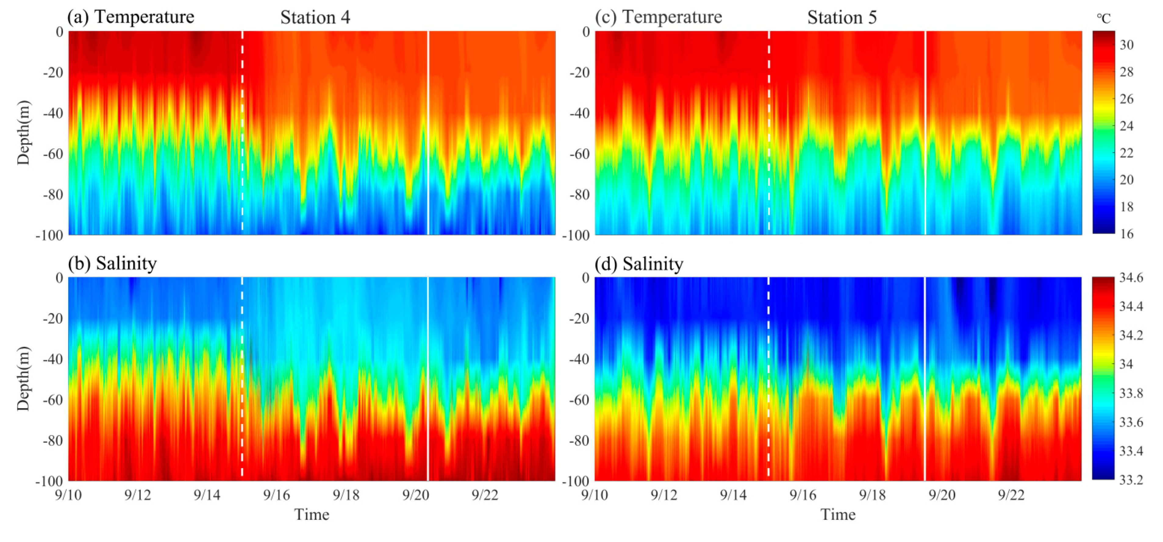
Figure 7a,b and Figure 8a–c show the changes of temperature and salinity in the upper ocean as well as that of the mixed layer before and after the sequential TCs at Station B4, which was located to the right of Kalmaegi but left of Fung-Wong. It can be seen that the increase in MLD and decrease in MLT influenced by Kalmaegi were much larger than that induced by Fung-Wong, whereas the MLS increased during Kalmaegi but then decreased during Fung-Wong. The differences in the variations of MLD, MLT and MLS caused by Kalmaegi and Fung-Wong were mainly due to the large difference in the MSW of the two TCs. The MSW of Kalmaegi ranged from 33 to 36 m s−1 when it passed over this region, while that of Fung-Wong was only 18 to 21 m s−1. In addition, the turning of wind stress to the right side of TC’s track may resonate with the near-inertial oscillations generated by a TC, which resulted in stronger vertical mixing [3,19]. Figure 7a,b shows that, the subsurface temperature at depth of ~50 to 100 m increased obviously, while the salinity above the depth of ~50 m increased first and then decreased after the two TCs. Compared with Figure 3c, the observations at Stations B4 and B5 reproduced the process of SST change measured from satellite, captured the two cooling events and the difference in cooling intensity as well.
Station B5 was located to the left side of both TCs’ tracks. As can be seen from Figure 7c,d and Figure 8d–f, compared with Station B4, the trends of MLD and MLT were similar but with weaker amplitudes, especially during the passage of Kalmaegi. There was no distinct change in MLS, probably because the salinity variation is constrained by many factors, such as precipitation and evaporation. It is worth mentioning that there was an obvious signal around September 16 that all isotherms within 200 m of the upper layer sank sharply (Figure 7c,d). This is possibly caused by the resonation between Kalmaegi-generated near-inertial oscillation and the internal wave, which could produce more energy and lead to stronger vertical mixing.
Consequently, the MLD deepened and MLT dropped after Kalmaegi or Fung-Wong, owing to the entrainment and upwelling induced by the TC. Meanwhile, the MLS increased on the right side of their tracks but decreased on the left side. The difference is mainly due to the asymmetry of precipitation (the figure is not shown) brought by the TC [46].
3.2. Biological Response
Figure 9 depicts the temporal evolution of surface chl-a concentration before, during and after the passages of Kalmaegi and Fung-Wong. Before TCs, the chl-a concentration in the SCS and CE region (region R1 in Figure 9) was a little higher than that in other areas of the WNP but fell within the predominant value of ≤ 0.1 mg m−3 in typical summer in SCS [12]. Not surprisingly, three typical regions with obvious surface cooling are also noted with pronounced growth of chl-a after sequential TCs. As mentioned in Section 3.1.1, the translation speed and intensity of the TCs were both conducive to chl-a rise when they passed over these three regions. However, the extent of enhancement varied from region to region due to the specific mechanisms involved.
Inside the CE (region R1), the maximum increase (0.21 mg m−3) in chl-a concentration occurred near the center of the eddy. Owing to the special thermodynamic structure of the CE, the subsurface water with rich nutrients inside the eddy would be more likely to be brought to the euphotic zone by TC-enhanced vertical mixing. Therefore, the pre-existing CE could not only modulate the thermodynamic response of the upper ocean, but also cause changes in biological processes.
As for the near-shore area (region R2), the average surface chl-a concentration increased from 0.38 to 0.53 mg m−3. At certain locations (e.g., 118.4°E, 20°N) of the coastal area, the chl-a concentration reached as high as 20 mg m−3. Except for the influence of translation speed and intensity of TCs, two other mechanisms may be responsible for this. (1) The depth of water in areas tens of kilometers offshore is usually only tens of meters [47], which make it easier to bring the nutrient from the lower layer to the surface. (2) The heavy rainfall caused by TCs can trigger the enrichment of terrigenous nutrients in near-shore waters.
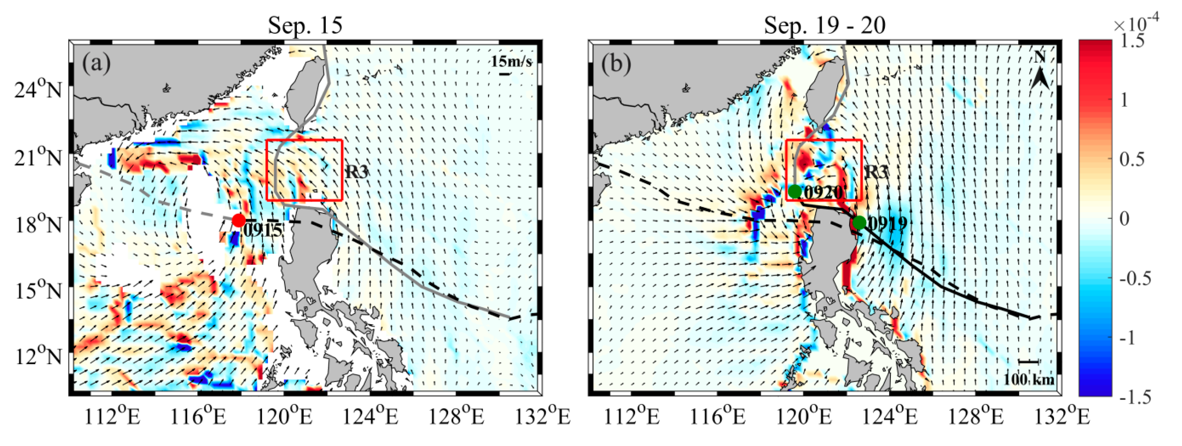
The peak value of chl-a rise in Luzon Strait (region R3) reached up to 0.58 mg m−3. The chl-a concentration even increased from 2.01 to 5.16 mg m−3 at the land-sea junction, demonstrating a prominent enhancement. It is noteworthy that the intensity of Fung-Wong had been continuously strengthened as it passed through this region during September 19 to 20. In addition to the mixing effect induced by sequential TCs, it can be observed from Figure 10 that both Kalmaegi and Fung-Wong caused strong upwelling with maximum EPV larger than 1.5×10⁴ m s−1, which is able to transport subsurface nutrients upward to the euphotic zone as well. Compared with the period from September 14 to 21, the response of chl-a during September 22 to 29 was more remarkable, probably related to the lag response of chl-a and the superposition effect of sequential TCs [11,21,48].
3.3. Influence of Sequential TCs on the CE
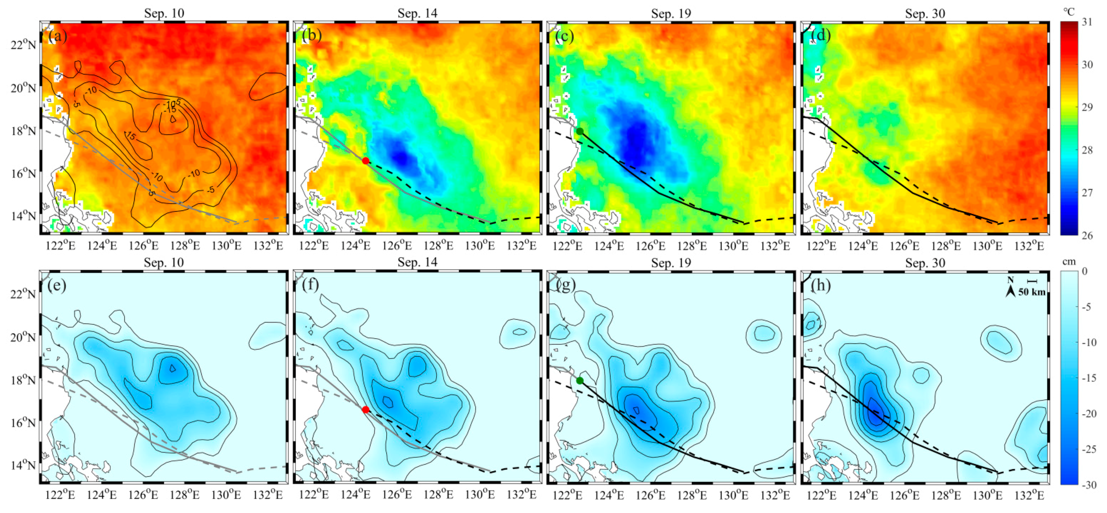
As mentioned in Section 3.1 and Section 3.2, the pre-existing CE has a significant impact on both the thermodynamic and biological responses of the upper ocean to TCs. Conversely, TCs could also influence the structure and intensity of the eddy. In this study, it is of interest that the CE region interacted with two TCs successively. Before Kalmaegi, the SST inside the CE was about 29.5 °C, not obviously lower than that of background waters (Figure 11a). On September 13 and 14 when Kalmaegi passed over the eddy, there was a significant decrease of 3.18 °C in SST (Figure 11b). During this period, the MSW ranged from 28.3 to 36.0 m s−1. The translation speed was higher than 6.0 m s−1, which is defined as a “fast-moving” TC [3]. The conditions were favorable for the formation of strong vertical mixing, especially to the right side of the TC’s track. After that, the water temperature gradually recovered but the process was then disturbed when Fung-Wong passed by. On September 19 when Fung-Wong left this area, a distinctly extreme cold patch was observed again in the CE region with a much stronger cooling of up to 3.28 °C compared to that on September 9 (Figure 11c). By September 30, more than 10 days, this cold patch was still evident (Figure 11d).
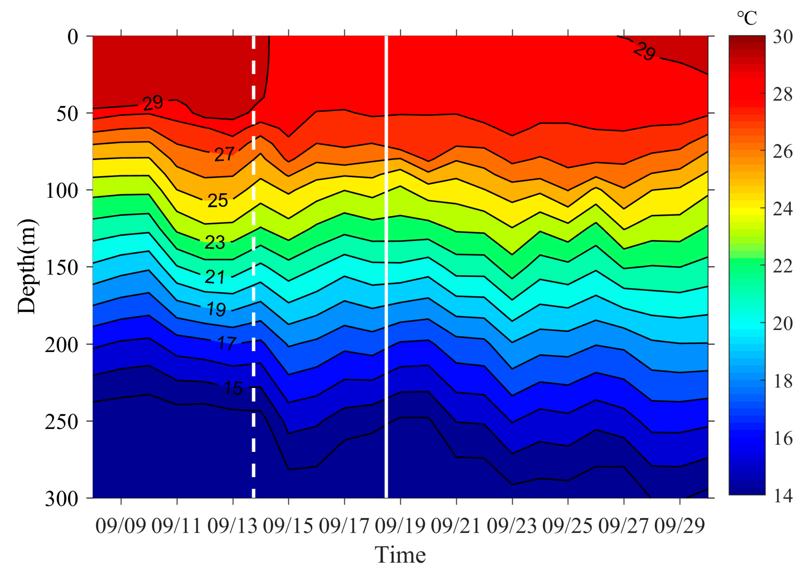
Figure 12 shows the variation of upper layer temperature at the eddy center. It can be seen that, the 29 °C isotherm, which was initially at a depth of ~50 m, rose rapidly to the surface on September 14 and outcropped after that until September 26. From September 14 to 15, all isotherms exhibited a downward trend. For example, the 27 °C isotherm deepened from the depth of ~60 m to ~80 m. These isotherms then rose slowly until the following TC Fung-Wong interacted with the eddy. Under the influence of the sequential TCs, the isotherms tended to descend as a whole, which means the vertical mixing effect plays a dominant role in the surface cooling of the CE region.
The intensity of a CE can be depicted by negative values of SSHA [49]. As shown in Figure 11, the SSHA at eddy center dropped by ~10 cm after the passage of Kalmaegi. Subsequently, Fung-Wong passed by and the SSHA dropped to the lowest value (~15 cm) by September 20. The northwestern part of the pre-existing CE was visibly strengthened by Fung-Wong and moved westward slightly. It is noted that the CE was intensified by both TCs although with varying degrees of impact, mainly because the MSW of Kalmaegi was twice that of Fung-Wong during this period.
3.4. Possible Causes of Sudden Track Change in Sequential TCs Scenario
In additional to the significant modulation on the ocean environment, sequential TCs usually result in an unusual track, as indicated by various studies [50,51,52]. As shown in Figure 1a, Fung-Wong shifted westward to the Luzon Strait following the prior TC Kalmaegi before September 20. However, Fung-Wong suddenly turned northward passing the eastern coast of the Taiwan Island. Is the sudden change of Fung-Wong’s track related to the prior TC Kalmaegi? This study tries to answer this question by analyzing both atmospheric and oceanic environments. First of all, tracks of TCs are mostly driven by large-scale steering flow in the middle troposphere. However, the TC-related circulation obscures the identification of the steering flow as the TCs are always embedded in complex environmental circulations. A TC-removal method, which was developed by Kurihara et al. (1993, 1995) [53,54], can objectively identify an asymmetric TC component to extract a smooth large-scale environmental field [55,56]. Using this TC-removal method, the background wind field, which represents the steering flow in the middle troposphere, is extracted to trace the TC’s movement.
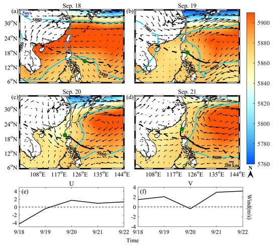
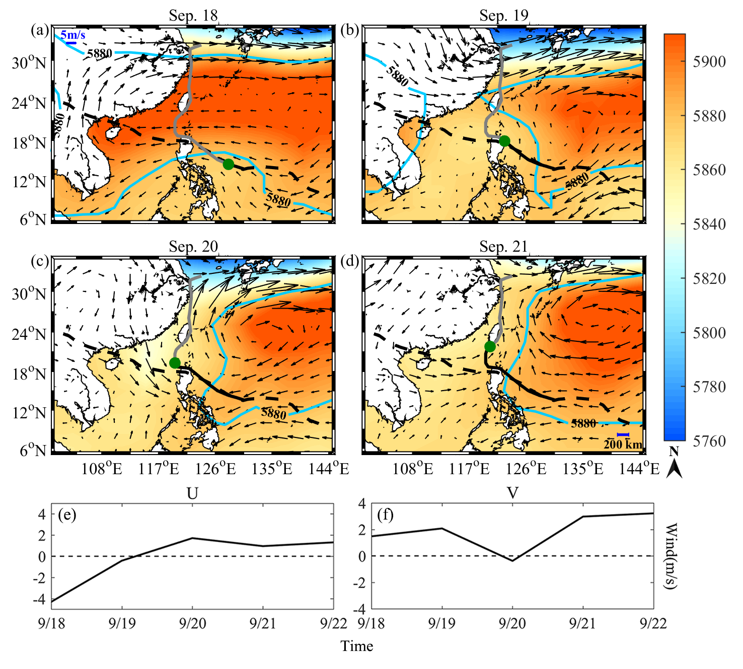
Variations of environment geopotential height and wind in the middle troposphere from September 18 to 21 are shown in Figure 13. On September 18, the western North Pacific subtropical high (WNPSH) was significantly strengthened with the 5880 gpm contour penetrating southward to approximately 10°N and dominated the entire tropical Northwestern Pacific (Figure 13a). Easterly prevailed to the south of the WNPSH and steered the TC Fung-Wong to the west. West of Fung-Wong, a significant ridge and a trough appeared over the SCS and the Philippine Island (Figure 13a). Such ridge and trough were related to the Rossby energy dispersion radiating from the prior TC Kalmaegi which had dissipated over the Indochina Peninsula [57,58]. Affected by the energy dispersion, the 5880 gpm contour to the south of the WNPSH wriggled sharply which resulted in a breakdown of the WNPSH. Thus, the trade easterly turned to northward since September 19 (Figure 13b–d). Meanwhile, Fung-Wong turned northward following the transition of the environment steering flow.
Figure 13e,f illustrate the variation of environmental flow steering the TC. The zonal steering flow changed from easterly to westerly during the period from September 18 to 20 (Figure 13e), preventing Fong-Wong from moving further westward. In particular, from September 19 to 20, weak steering flow corresponded with the slow translation speed (less than 4 m s−1) of Fung-Wong. The northward steering flow suddenly strengthened during September 20, resulting in poleward acceleration of Fung-Wong (Figure 13f). The zonal steering flow was about twice as strong as the meridional flow before September 19 but the meridional steering flow dominated after September 20. Thus, the sudden northward turning of Fung-Wong is attributed to the abrupt change of the environmental flow in association with the Rossby energy dispersion of the prior TC Kalmaegi.
This pattern aroused the conceptual model of Carr et al. (1977) [59]. However, the critical differences exist between this event and Carr’s model. According to Carr’s model, the WNPSH was located to the north of the subsequent TC. Combined with the Rossby wave dispersion-induced anticyclone to the east and equatorward of the prior TC, it will impose an equatorward environmental flow steering the following TC southwest. In this case, the trade easterly to the south of the WNPSH penetrated further equatorward. Modulated by the Rossby wave, the northward steering flow formed and steered the subsequent TC poleward. The differences in the location of the WNPSH are the key for the opposite moving direction of the subsequent TC between Carr’s model and this event.
In addition to the favorable atmospheric conditions, oceanic factors are also likely to affect the northward turning of Fung-Wong. Figure 14 displays the distributions of some ocean environmental variables on September 19, i.e., before Fung-Wong turned to the north. It is found that SST in the SCS dropped obviously after Kalmaegi. It was only ~28.4 °C and lower than SST in Luzon Strait and the coastal region of Taiwan Island. Simultaneously, lower UOHC, shallower MLD and D26 were also observed in the SCS. It is believed that the maintenance of a mature TC requires heat energy supplement pumping from the warm ocean. Apparently, the ocean conditions in the SCS were not favorable for the maintenance of a TC. Thus, we speculate that Fung-Wong tended to move to areas with warmer ocean conditions other than shifting further westward into the colder SCS.
4. Conclusions
The combination of satellite data, numerical model outputs and in situ observations provides a unique opportunity to study the influence of TCs on the upper ocean. In this paper, multi-platform datasets were used to investigate the thermodynamic and biological responses of the upper ocean to two sequential TCs over the NWP, i.e., Kalmaegi and Fung-Wong in 2014. The possible causes of the sudden change of Fung-Wong’s track were also explored considering both atmospheric and oceanic environments.
After two TCs passed by, the SST significantly decreased due to the strong oceanic entrainment and upwelling. Three distinct cold patches were observed along their tracks. The magnitude and extent of sea surface cooling are not only highly related to the intensity and translation speed of the TC, but also associated with the ocean background environments (e.g., MLD, D26 and UOHC). Double TCs had superimposed effects on the upper ocean. They deepened the mixing layer and lower the MLT at the same time. The change of MLD or MLT on the right side of the TC’s track was stronger than that on the left. The MLS showed a different trend, with a decrease on the left side of the TC but an increase on the right. Meanwhile, it is found that the surface chl-a concentration was enhanced by the TCs. The areas with particularly pronounced chl-a enhancement coincided well with surface cooling regions.
The pre-existing CE plays a notable role in modulating both thermodynamic and biological responses of the upper ocean owing to its unique and relatively unstable thermodynamic structure. On the other hand, it was significantly influenced by the TCs. The CE was enhanced with SST drop of 3.28 °C and SSHA decline of ~15 cm.
The present work indicated that the prior TC can affect the track of the subsequent TC by changing the atmospheric and ocean environments. The mature TC Kalmaegi radiated a Rossby wave energy southeastward which wriggled the environmental flow to the south of WNPSH. Consequently, the steering flow changed from westward to northward, leading to the abrupt northward turning of Fung-Wong.
For another aspect, the possible impact of ocean environment on the movement of the TC was also pointed out. With lower UOHC, shallower MLD and D26, the colder SCS could not supply Fung-Wong with enough energy, which can help explain why Fung-Wong did not continue to move westward into the SCS but suddenly turned to the north.
Although under different ocean background conditions, the upper ocean responses to TCs may differ, TC-induced strong upwelling and vertical mixing are the main factors that influence upper ocean conditions. Thus the main findings of this study, including sea surface cooling, chlorophyll enhancement, and subsurface warming, could shed light on one of the general behaviors of the upper ocean responses to TCs. Furthermore, the effect of atmospheric and oceanic environmental changes accompanying the prior TC on the characteristics of the following TC is highlighted, which may provide important insights into the forecasting of the TC’s track in sequential TCs scenario. Nevertheless, further studies are needed to improve our understanding of the relationship between the two sequential TCs and their interaction with the ocean by combining the coupled ocean-atmosphere numerical model with current observations.
Author Contributions
Conceptualization, J.N. and Q.X.; methodology, J.N. and Q.X.; software, J.N.; validation, J.N. and Q.X.; formal analysis, J.N.; investigation, J.N., Q.X. and T.F.; data curation, J.N., H.Z. and T.F.; writing—original draft preparation, J.N.; writing—review and editing, Q.X., T.F., H.Z., T.W.; supervision, Q.X., T.F. and T.W.
Funding
This research was funded by the National Key Project of Research and Development Plan of China (Grant No. 2016YFC1401905), the Fundamental Research Funds for the Central Universities (Hohai University) (Grant Nos. 2019B18714 and 2018B702X14), the Postgraduate Research & Practice Innovation Program of Jiangsu Province (Grant No. KYCX18_0523), Dayu Scholar Program of Hohai University (for Q. Xu), the National Natural Science Foundation of China (Grant Nos. 41976163 and 41706002), and the National Program on Global Change and Air–Sea Interaction (Grant No. GASI-IPOVAI-04).
Acknowledgments
The authors thank the editor and the anonymous reviewers for their constructive comments which help to improve the paper. We acknowledge the Joint Typhoon Warming Center (JTWC) for providing Typhoon information (http://www.usno.navy.mil/NOOC/nmfc-ph/RSS/jtwc/best_tracks), the Remote Sensing Systems for providing the SST data (http://www.remss.com/), the Copernicus Marine and Environment Monitoring Service (CMEMS) database for providing the SSHA dataset (http://marine.Coperni cus.eu/), the GlobColour Project for providing the chl data (http://hermes.acri.fr/), the NOAA’s National Climatic Data Center for providing the ocean surface winds (http://www.ncdc.noaa.gov/oa/rsad/air-sea/seawinds.html), the China Argo Real-time Data Center for providing the Argo data (http://www.argo.org.cn/), the Hybrid Coordinate Ocean Model (HYCOM) for providing the ocean analysis data (https://www.hycom.org/), and the NCEP–DOE AMIP-II Reanalysis for providing the atmospheric fields data.
Conflicts of Interest
The authors declare no conflict of interest.
References
- Emanuel, K. Tropical Cyclones. Annu. Rev. Earth Planet. Sci. 2003, 31, 75–104. [Google Scholar] [CrossRef]
- Greatbatch, R.J. On the response of the ocean to a moving storm: Parameters and scales. J. Phys. Oceanogr. 1984, 14, 59–78. [Google Scholar] [CrossRef]
- Price, J.F. Upper ocean response to a Hurricane. J. Phys. Oceanogr. 1981, 11, 153–175. [Google Scholar] [CrossRef]
- Price, J.F.; Sanford, T.B.; Forristall, G.Z. Forced stage response to a moving hurricane. J. Phys. Oceanogr. 1994, 24, 233–260. [Google Scholar] [CrossRef]
- D’Asaro, E.A.; Sanford, T.B.; Niiler, P.P.; Terrill, E.J. Cold wake of Hurricane Frances. Geophys. Res. Lett. 2007, 34, 15609. [Google Scholar] [CrossRef]
- Zheng, Z.W.; Ho, C.R.; Zheng, Q.A.; Lo, Y.T.; Kuo, N.J.; Gopalakrishnan, G. Effects of preexisting cyclonic eddies on upper ocean responses to Category 5 typhoons in the western north pacific. J. Geophys. Res. Oceans 2010, 115. [Google Scholar] [CrossRef]
- Zheng, Z.W.; Ho, C.R.; Kuo, N.J. Importance of pre-existing oceanic conditions to upper ocean response induced by Super Typhoon Hai-Tang. Geophys. Res. Lett. 2008, 35, 288–299. [Google Scholar] [CrossRef]
- Ning, J.; Xu, Q.; Zhang, H.; Wang, T.; Fan, K. Impact of cyclonic ocean eddies on upper ocean thermodynamic response to Typhoon Soudelor. Remote Sens. 2019, 11, 938. [Google Scholar] [CrossRef]
- Ning, J.; Xu, Q.; Wang, T.; Zhang, S.S. Upper ocean response to Super Typhoon Soudelor revealed by different SST products. IGARSS 2018, 6063–6066. [Google Scholar] [CrossRef]
- Lin, I.I.; Wu, C.C.; Pun, I.F.; Ko, D.S. Upper-ocean thermal structure and the western North Pacific Category 5 typhoons. Part 1: Ocean features and the Category 5 typhoons’ intensification. Mon. Weather Rev. 2008, 136, 3288–3306. [Google Scholar] [CrossRef]
- Wu, R.H.; Li, C.Y. Upper ocean response to the passage of two sequential typhoons. Deep Sea Res. 2018, 132, 68–79. [Google Scholar] [CrossRef]
- Lin, I.I.; Liu, W.T.; Wu, C.C.; Wong, G.T.F.; Hu, C.; Zhen, Z.; Liang, W.D.; Yang, Y.; Liu, K.K. New evidence for enhanced ocean primary production triggered by tropical cyclone. Geophys. Res. Lett. 2003, 30, 1718. [Google Scholar] [CrossRef]
- Zhao, H.; Tang, D.L.; Wang, D. Phytoplankton blooms near the Pearl river estuary induced by typhoon nuri. J. Geophys. Res. Oceans 2009, 114. [Google Scholar] [CrossRef]
- Schade, L.R.; Emanuel, K.A. The ocean’s effect on the intensity of tropical cyclones: Results from a simple coupled atmosphere–ocean model. J. Atmos. Sci. 1999, 56, 642–651. [Google Scholar] [CrossRef]
- Jaimes, B.; Shay, L.K. Mixed layer cooling in mesoscale oceanic eddies during hurricanes Katrina and Rita. Mon. Weather Rev. 2009, 137, 4188–4207. [Google Scholar] [CrossRef]
- Pan, J.Y.; Huang, L.; Devlin, A.T.; Lin, H. Quantification of typhoon-induced phytoplankton blooms using satellite multi-sensor data. Remote Sens. 2018, 10, 318. [Google Scholar] [CrossRef]
- Sanford, T.B.; Price, J.F.; Girton, J.B. Upper-ocean response to Hurricane Frances (2004) observed by profiling EM-APEX floats. J. Phys. Oceanogr. 2011, 41, 1041–1056. [Google Scholar] [CrossRef]
- Zhang, H.; Wu, R.; Chen, D.K.; Liu, X.H.; He, H.; Tang, Y.; Ke, D.; Shen, Z.; Li, J.; Xie, J.; et al. Net modulation of upper ocean thermal structure by Typhoon Kalmaegi (2014). J. Geophys. Res. Oceans 2018, 123, 7154–7171. [Google Scholar] [CrossRef]
- Zhang, H.; Chen, D.K.; Zhou, L.; Liu, X.H.; Ding, T.; Zhou, B. Upper ocean response to Typhoon Kalmaegi (2014). J. Geophys. Res. Oceans 2016, 121, 6520–6535. [Google Scholar] [CrossRef]
- Ko, D.S.; Chao, S.Y.; Wu, C.C.; Lin, I.I. Impacts of Typhoon Megi (2010) on the South China Sea. J. Geophys. Res. Oceans 2014, 119, 4474–4489. [Google Scholar] [CrossRef]
- Walker, N.D.; Leben, R.R.; Balasubramanian, S. Hurricane-forced upwelling and chlorophyll a, enhancement within cold-core cyclones in the Gulf of Mexico. Geophys. Res. Lett. 2005, 32, 18610. [Google Scholar] [CrossRef]
- Shang, X.D.; Zhu, H.B.; Chen, G.Y.; Xu, C.; Yang, Q. Research on cold core eddy change and phytoplankton bloom induced by typhoons: Case studies in the South China Sea. Adv. Meteorol. 2015, 1–19. [Google Scholar] [CrossRef]
- Sun, L.; Li, Y.X.; Yang, Y.J.; Wu, Q.; Chen, X.T.; Li, Q.Y.; Li, Y.B.; Xian, T. Effects of super typhoons on cyclonic ocean eddies in the western North Pacific: A satellite data-based evaluation between 2000 and 2008. J. Geophys. Res. Oceans 2014, 119, 5585–5598. [Google Scholar] [CrossRef]
- Lu, Z.; Wang, G.; Shang, X.D. Response of a pre-existing cyclonic ocean eddy to a typhoon. J. Phys. Oceanogr. 2016, 46, 2403–2410. [Google Scholar] [CrossRef]
- Jin, F.F.; Boucharel, J.; Lin, I.I. Eastern Pacific tropical cyclones intensified by El Niño delivery of subsurface ocean heat. Nature 2014, 516, 82–85. [Google Scholar] [CrossRef]
- Chen, D.K.; Lei, X.T.; Wang, W.; Wang, G.H.; Han, G.J.; Zhou, L. Upper ocean response and feedback mechanisms to typhoon (in Chinese). Adv. Earth Sci. 2013, 28, 1077–1086. [Google Scholar] [CrossRef]
- Jarrell, J.; Brand, S.; Nicklin, D.S. An analysis of western North Pacific tropical cyclone forecast errors. Mon. Weather Rev. 1978, 106, 925–937. [Google Scholar] [CrossRef]
- Wu, X.; Fei, J.F.; Huang, X.G.; Zhang, X.; Cheng, X.P.; Ren, J.Q. A numerical study of the interaction between two simultaneous storms: Goni and Morakot in September 2009. Adv. Atmos. Sci. 2012, 29, 561–574. [Google Scholar] [CrossRef]
- Wu, C.C.; Emanuel, K.A. Potential vorticity diagnostics of hurricane movement. Part 1: A case study of Hurricane Bob (1991). Mon. Weather Rev. 1995, 123, 69–92. [Google Scholar] [CrossRef]
- Chan, J.C.L. The physics of tropical cyclone motion. Annu. Rev. Fluid Mech. 2005, 37, 99–128. [Google Scholar] [CrossRef]
- Wu, L.; Wang, B.; Braun, S.A. Impacts of air–sea interaction on tropical cyclone track and intensity. Mon. Weather Rev. 2005, 133, 3299–3314. [Google Scholar] [CrossRef]
- Yun, K.S.; Chan, J.C.L.; Ha, K.J. Effects of SST magnitude and gradient on typhoon tracks around East Asia: A case study for Typhoon Maemi (2003). Atmos. Res. 2012, 109, 36–51. [Google Scholar] [CrossRef]
- Wada, A.; Usui, N.; Sato, K. Relationship of maximum tropical cyclone intensity to sea surface temperature and tropical cyclone heat potential in the North Pacific Ocean. J. Geophys. Res. 2012, 117, D11118. [Google Scholar] [CrossRef]
- Wu, L.; Zhao, H. Dynamically derived tropical cyclone intensity changes over the western North Pacific. J. Clim. 2012, 25, 89–98. [Google Scholar] [CrossRef]
- Gentemann, C.L. Near real time global optimum interpolated microwave SSTs: Applications to hurricane intensity forecasting. In Proceedings of the 26th Conference on Hurricanes and Tropical Meteorology, Miami, FL, USA, 2–7 May 2004. [Google Scholar]
- Reynolds, R.W.; Smith, T.M. Improved global sea surface temperature analyses using optimum interpolation. J. Clim. 1994, 7, 929–948. [Google Scholar] [CrossRef]
- Peng, G.; Zhang, H.M.; Frank, H.P.; Bidlot, J.R.; Hanjins, A.W.R. Evaluation of various surface wind products with oceanSITES buoy measurements. Weather Forecast. 2013, 28, 1281–1303. [Google Scholar] [CrossRef]
- Liu, Z.H. Global Ocean Argo Scatter Data Set (V2.1) (1996/01-2017/05) User Manual (in Chinese); China Argo Real-time Data Center: Hangzhou, China, 2017. [Google Scholar]
- Chassignet, E.P.; Hurlburt, H.E.; Smedstad, O.M.; Halliwell, G.R.; Hogan, P.J.; Wallcraft, A.J.; Baraille, R.; Bleck, R. The HYCOM (HYbrid Coordinate Ocean Model) data assimilative system. J. Mar. Syst. 2007, 65, 60–83. [Google Scholar] [CrossRef]
- Kanamitsu, M.; Ebisuzaki, W.; Woollen, J.; Yang, S.K.; Hnilo, J.J.; Fiorino, M.; Potter, G.L. NCEP–DOE AMIP-II Reanalysis (R-2). Bull. Am. Meteorol. Soc. 2002, 83, 1631–1643. [Google Scholar] [CrossRef]
- Kara, A.B.; Rochford, P.A.; Hurlburt, H.E. An optimal definition for ocean mixed layer depth. J. Geophys. Res. Oceans 2000, 105, 16803–16821. [Google Scholar] [CrossRef]
- Garratt, J.R. Review of drag coefficients over oceans and continents. Mon. Weather Rev. 1997, 105, 915–929. [Google Scholar] [CrossRef]
- Oey, L.Y.; Ezer, T.; Wang, D.P.; Fan, S.J.; Yin, X.Q. Loop current warming by Hurricane Wilma. Geophys. Res. Lett. 2006, 33, L08613. [Google Scholar] [CrossRef]
- Large, W.G.; Pond, S. Open ocean momentum flux measurements in moderate to strong winds. J. Phys. Oceanogr. 1981, 11, 324–336. [Google Scholar] [CrossRef]
- Powell, M.D.; Vickery, P.J.; Reinhold, T. Reduced drag coefficient for high wind speeds in tropical cyclones. Nature 2003, 422, 279–283. [Google Scholar] [CrossRef] [PubMed]
- Chen, S.S.; Knaff, J.A.; Marks, F.D. Effects of vertical wind shear and storm motion on tropical cyclone rainfall asymmetries deduced from TRMM. Mon. Weather Rev. 2006, 134, 3190–3208. [Google Scholar] [CrossRef]
- Zhao, H.; Qi, Y.Q.; Wang, D.X.; Wang, W.Z. Study on the features of chlorophyll a derived from SeaWiFS in the South China Sea (in Chinese). Acta Oceanol. Sin. 2005, 27, 45–52. [Google Scholar] [CrossRef]
- Zheng, G.M.; Tang, D.L. Offshore and nearshore chlorophyll increases induced by typhoon winds and subsequent terrestrial rainwater runoff. Mar. Ecol. Prog. Ser. 2007, 333, 61–74. [Google Scholar] [CrossRef] [Green Version]
- Chelton, D.B.; Gaube, P.; Schlax, M.G.; Early, J.J.; Samelson, R.M. The influence of nonlinear mesoscale eddies on near-surface oceanic chlorophyll. Science 2011, 334, 328–332. [Google Scholar] [CrossRef]
- Prieto, R.; McNoldy, B.D.; Fulton, S.R.; Schubert, W.H. A classification of binary tropical cyclone–like vortex interactions. Mon. Weather Rev. 2003, 131, 2656–2666. [Google Scholar] [CrossRef]
- Wu, C.C.; Huang, T.S.; Huang, W.P.; Chou, K.H. A new look at the binary interaction: Potential vorticity diagnosis of the unusual southward movement of Tropical Storm Bopha (2000) and its interaction with Supertyphoon Saomai (2000). Mon. Weather Rev. 2003, 131, 1289–1300. [Google Scholar] [CrossRef]
- Jang, W.; Chun, H.Y. Characteristics of binary tropical cyclones observed in the western North Pacific for 62 years (1951–2012). Mon. Weather Rev. 2015, 143, 1749–1761. [Google Scholar] [CrossRef]
- Kurihara, Y.; Bender, M.A.; Ross, R.J. An initialization scheme of hurricane models by vortex specification. Mon. Weather Rev. 1993, 121, 2030–2045. [Google Scholar] [CrossRef]
- Kurihara, Y.; Bender, M.A.; Tuleya, R.E.; Ross, R.J. Improvements in the GFDL hurricane prediction system. Mon. Weather Rev. 1995, 123, 2791–2801. [Google Scholar] [CrossRef]
- Hsu, H.H.; Hung, C.H.; Lo, A.K.; Wu, C.C.; Hung, C.W. Influence of tropical cyclones on the estimation of climate variability in the tropical western North Pacific. J. Clim. 2008, 21, 2960–2975. [Google Scholar] [CrossRef]
- Cao, X.; Wu, R.; Bi, M. Contributions of different time-scale variations to tropical cyclogenesis over the western North Pacific. J. Clim. 2018, 31, 3137–3153. [Google Scholar] [CrossRef]
- Ritchie, E.A.; Holland, G.J. Large-scale patterns associated with tropical cyclogenesis in the western Pacific. Mon. Weather Rev. 1999, 127, 2027–2043. [Google Scholar] [CrossRef]
- Li, T.; Fu, B. Tropical cyclogenesis associated with Rossby wave energy dispersion of a preexisting typhoon. Part I: Satellite data analyses. J. Atmos. Sci. 2006, 63, 1377–1389. [Google Scholar] [CrossRef]
- Carr, L.E.; Boother, M.A.; Elsberry, R.L. Observational evidence for alternate modes of track-altering binary tropical cyclone scenarios. Mon. Weather Rev. 1997, 125, 2094–2111. [Google Scholar] [CrossRef]
Figure 1.
The tracks (a), intensities (b,c), and translation speeds (d,e) of Kalmaegi (left panel) and Fung-Wong (right panel). The blue and red dashed lines indicate tracks of Kalmaegi and Fung-Wong, respectively. The symbol “*” in (a) denotes the center location of two TCs at 00:00 UTC on the corresponding date. The black triangles with symbols from “B1” to “B5” indicate five array stations. The magenta pentagrams with symbols “A1” and “A2” indicate the locations of the two Argo floats.

Figure 2.
Comparisons of SST, SSTD and SSHA between satellite observations (Top) and HYCOM data (Bottom). (a,b): SST distributions before Kalmaegi, (c,d): SSTD during the passage of Kalmaegi (i.e., SST difference between September 15 and 9), (e,f): negative SSHA in the area denoted by the blue box in (c) before Kalmaegi. The dash and solid lines denote the tracks of Kalmaegi and Fung-Wong, respectively. The black and gray parts of the lines represent the TC has and has not passed the region, respectively. The red dot denotes the center location of Kalmaegi at 00:00 UTC on September 15.

Figure 3.
Satellite observed evolution of SST before, during and after Kalmaegi and Fung-Wong. (a): before Kalmaegi, (b,c): during Kalmaegi and before Fung-Wong, (d–f): after Kalmaegi and during Fung-Wong. The expression of TC tracks is the same as Figure 2. The red and green dots denote the center locations of Kalmaegi and Fung-Wong at 00:00 UTC, respectively. The black, gray and red boxes represent typical regions with distinct sea surface cooling.

Figure 4.
Spatial distributions of MLD, D26 and UOHC from HYCOM output before the formation of Kalmaegi on September 9 (upper panel) and Fung-Wong on September 17 (lower panel). (a,b): MLD, (c,d): D26, (e,f): UOHC. The expression of TC tracks is the same as Figure 2. The red dot denotes the center location of Kalmaegi at 00:00 UTC on September 17.

Figure 5.
Distribution of SSTD during the passages of Kalmaegi on September 14 (i.e., SST difference between September 14 and 9) (a) and Fung-Wong on September 19 (i.e., SST difference between September 19 and 9) (b). Overlaid is SSHA (contours, unit: cm) on the corresponding date. Only negative values are plotted, with closed contours indicating the location of the CE. The expression of TC tracks is the same as Figure 2. The red and green dots denote the center locations at 00:00 UTC of Kalmaegi and Fung-Wong, respectively.

Figure 6.
Temperature and salinity profiles observed by Argo floats A1 (Top, (a,b)) and A2 (Bottom, (c,d)). Curves with different colours represent observations on different dates.
Figure 6.
Temperature and salinity profiles observed by Argo floats A1 (Top, (a,b)) and A2 (Bottom, (c,d)). Curves with different colours represent observations on different dates.

Figure 7.
Variations of temperature (Top, (a,c)) and salinity (Bottom, (b,d)) vertical profiles at Stations B4 (Left) and B5 (Right). The dashed and solid vertical straight lines denote the time when Kalmaegi and Fung-Wong passed by, respectively.
Figure 7.
Variations of temperature (Top, (a,c)) and salinity (Bottom, (b,d)) vertical profiles at Stations B4 (Left) and B5 (Right). The dashed and solid vertical straight lines denote the time when Kalmaegi and Fung-Wong passed by, respectively.

Figure 8.
Variations of MLD (Top, (a,d)), MLT (Middle, (b,e)), and MLS (Bottom, (c,f)) at Stations B4 (Left) and B5 (Right). The dashed and solid vertical straight lines denote the time when Kalmaegi and Fung-Wong passed by, respectively.
Figure 8.
Variations of MLD (Top, (a,d)), MLT (Middle, (b,e)), and MLS (Bottom, (c,f)) at Stations B4 (Left) and B5 (Right). The dashed and solid vertical straight lines denote the time when Kalmaegi and Fung-Wong passed by, respectively.

Figure 9.
Satellite observed evolution of surface chl-a concentration (mg m−3) before (a), during (b) and after (c) sequential TCs. The expression of TC tracks is the same as Figure 2. The black, gray and red boxes represent three typical regions with obvious chl-a increase and surface cooling as well as shown in Figure 3.

Figure 10.
The wind field (arrows; m s−1) at 10 m above sea surface and estimated EPV (colours; m s−1) on September 15 (a), 19 and 20 (b). The expression of TC tracks is the same as Figure 2. The red and green dots denote the center locations of Kalmaegi and Fung-Wong at 00:00 UTC, respectively. The red box represents region R3 depicted in Figure 9.

Figure 11.
Evolution of satellite observed SST (Top, (a–d)) and negative SSHA (Bottom, (e–h)) in the CE region before, during and after sequential TCs. The expression of TC tracks is the same as Figure 2. The red and green dots denote the center locations of Kalmaegi and Fung-Wong at 00:00 UTC, respectively.

Figure 12.
HYCOM output of temperature profile at the center of the CE on September 9. The dash and solid lines denote the time when Kalmaegi and Fung-Wong passed by the eddy, respectively.
Figure 12.
HYCOM output of temperature profile at the center of the CE on September 9. The dash and solid lines denote the time when Kalmaegi and Fung-Wong passed by the eddy, respectively.

Figure 13.
500 hPa geopotential height (colour; gpm) and wind field (black arrows; m s−1) averaged at 500–700 hPa. Spatial distributions of 500 hPa geopotential height and wind field averaged at 500–700 hPa before (a,b), during (c) and after (d) the change of Fung-Wong’s track. The cyan line indicates the value of the geopotential height of 5880 gpm at 500 hPa. The expression of TC tracks is the same as Figure 2. The green dot denotes the center location at 00:00 UTC of Fung-Wong. (e,f) are temporal variations of zonal and meridional wind speed averaged at 500–700 hPa in a 5° × 5° region centered at Fung-Wong’s center location, respectively. Positive values of U and V denote the eastward and northward winds, respectively.

Figure 14.
Distributions of SST (a), MLD (b), D26 (c) and UOHC (d) on September 19. The expression of TC tracks is the same as Figure 2. The green dot denotes the center location at 00:00 UTC of Fung-Wong.
Figure 14.
Distributions of SST (a), MLD (b), D26 (c) and UOHC (d) on September 19. The expression of TC tracks is the same as Figure 2. The green dot denotes the center location at 00:00 UTC of Fung-Wong.


Table 1.
The locations of Argo floats and variations of MLD, MLT and MLS.
| Float | Location (°) | Date | MLD (m) | MLT (°C) | MLS |
|---|---|---|---|---|---|
| A1 | (119.28 E, 17.90 N) | Sep. 11 | 42.5 | 29.41 | 33.14 |
| (119.41 E, 17.97 N) | Sep. 15 | 42.5 | 28.45 | 33.29 | |
| (119.44 E, 17.93 N) | Sep. 19 | 37.5 | 28.65 | 33.07 | |
| (119.69 E, 18.09 N) | Sep. 23 | 47.5 | 28.25 | 33.11 | |
| A2 | (116.72 E, 16.86 N) | Sep. 11 | 35.5 | 29.26 | 33.34 |
| (116.84 E, 16.99 N) | Sep. 15 | 36.5 | 28.84 | 33.18 | |
| (116.93 E, 16.92 N) | Sep. 19 | 45.5 | 28.68 | 33.14 | |
| (116.95 E, 16.87 N) | Sep. 23 | 40.5 | 28.34 | 32.97 |
© 2019 by the authors. Licensee MDPI, Basel, Switzerland. This article is an open access article distributed under the terms and conditions of the Creative Commons Attribution (CC BY) license (http://creativecommons.org/licenses/by/4.0/).
Share and Cite
MDPI and ACS Style
Ning, J.; Xu, Q.; Feng, T.; Zhang, H.; Wang, T. Upper Ocean Response to Two Sequential Tropical Cyclones over the Northwestern Pacific Ocean. Remote Sens. 2019, 11, 2431. https://0-doi-org.brum.beds.ac.uk/10.3390/rs11202431
AMA Style
Ning J, Xu Q, Feng T, Zhang H, Wang T. Upper Ocean Response to Two Sequential Tropical Cyclones over the Northwestern Pacific Ocean. Remote Sensing. 2019; 11(20):2431. https://0-doi-org.brum.beds.ac.uk/10.3390/rs11202431
Chicago/Turabian StyleNing, Jue, Qing Xu, Tao Feng, Han Zhang, and Tao Wang. 2019. "Upper Ocean Response to Two Sequential Tropical Cyclones over the Northwestern Pacific Ocean" Remote Sensing 11, no. 20: 2431. https://0-doi-org.brum.beds.ac.uk/10.3390/rs11202431
Note that from the first issue of 2016, this journal uses article numbers instead of page numbers. See further details here.