Ultrasonic Proximal Sensing of Pasture Biomass


1
Department of Mechanical and Electrical Engineering, Massey University, 229 Dairy Flat Highway, Auckland 0632, New Zealand
2
Inverse Acoustics Ltd., 2 Rata Street, Auckland 0600, New Zealand
*
Author to whom correspondence should be addressed.
Remote Sens. 2019, 11(20), 2459; https://0-doi-org.brum.beds.ac.uk/10.3390/rs11202459
Submission received: 5 September 2019
/
Revised: 19 October 2019
/
Accepted: 21 October 2019
/
Published: 22 October 2019
(This article belongs to the Special Issue Advances of Remote Sensing in Pasture Management)
Abstract
:The optimization of pasture food value, known as ‘biomass’, is crucial in the management of the farming of grazing animals and in improving food production for the future. Optical sensing methods, particularly from satellite platforms, provide relatively inexpensive and frequently updated wide-area coverage for monitoring biomass and other forage properties. However, there are also benefits from direct or proximal sensing methods for higher accuracy, more immediate results, and for continuous updates when cloud cover precludes satellite measurements. Direct measurement, by cutting and weighing the pasture, is destructive, and may not give results representative of a larger area of pasture. Proximal sensing methods may also suffer from sampling small areas, and can be generally inaccurate. A new proximal methodology is described here, in which low-frequency ultrasound is used as a sonar to obtain a measure of the vertical variation of the pasture density between the top of the pasture and the ground and to relate this to biomass. The instrument is designed to operate from a farm vehicle moving at up to 20 km h−1, thus allowing a farmer to obtain wide coverage in the normal course of farm operations. This is the only method providing detailed biomass profile information from throughout the entire pasture canopy. An essential feature is the identification of features from the ultrasonic reflectance, which can be related sensibly to biomass, thereby generating a physically-based regression model. The result is significantly improved estimation of pasture biomass, in comparison with other proximal methods. Comparing remotely sensed biomass to the biomass measured via cutting and weighing gives coefficients of determination, R2, in the range of 0.7 to 0.8 for a range of pastures and when operating the farm vehicle at speeds of up to 20 km h−1.

1. Introduction
Biomass describes the food value of pasture for grazing animals. It is the ‘dry matter’ (DM) weight, per unit area of land, resulting when the pasture is cut to the ground, dried, and weighed [1]. Biomass is therefore an areal density, measured in kg m−2 or kg ha−1 (a hectare is 104 m2). Increasing the dry matter of perennial forages remains a crucial factor underpinning the profitability of grazing industries [2].
Pasture biomass may be measured by cutting, drying, and weighing quadrants of pasture. However, this is destructive and time-consuming, as well as unlikely to give information representative of a larger area of pasture. Therefore, this direct evaluation is generally only used for the detailed calibration of other methods. Satellite, aerial, and ground-based platforms equipped with advanced sensors provide the potential for fast, non-destructive, and low-cost monitoring of plant growth, development, and yield in a field environment [3]. The methods currently used include the measurement of parameters such as capacitance, spectral properties, pasture height (known as sward height), and compressed sward height [4,5,6,7,8,9,10,11,12]. A wide range of optical sensors have been used to measure a range of parameters of crops and pastures, including biomass [9,10,11,12,13,14,15,16,17,18,19,20,21,22]. Vegetation indices are obtained through combinations of back-scattered intensities recorded at various wavelengths [13]. However, pasture is often optically thick, which is evident from casual visual observation, so that back-scattered light may be predominantly from the upper levels of the pasture. This means that optical reflections from pasture of high biomass may not appear very different to optical reflections from pasture of medium biomass [16,17,18]. Modified versions of NDVI (Normalized Difference Vegetation Index) have been developed to reduce this saturation effect [17,19] and improved biomass estimation accuracy has also been reported when NDVI measurements are combined with pasture height measurements [15]. Furthermore, the use of a wider range of optical wavelengths, including new wavelength bands on the Sentinel-2 satellite platform, together with radiative models, reduces the optical saturation effects [19,23,24,25]. Satellite platforms are therefore able to produce wide coverage information at relatively low cost and repetition rates, and with considerable scope for detail because of the spectral range which penetrates the atmosphere. Nevertheless, there are also benefits from proximal sensing (near ground level), because proximal sensing gives immediate data to the farmer under their control and with potentially higher accuracy. Such proximal sensing is complementary to satellite sensing. The current work describes a new proximal sensor, and satellite and airborne methods will not be discussed in detail. However, for more information, the reader is referred to review papers such as those provided in references [3,6,7,8,9,11,12,13,14].
Pasture height may be measured manually using a tape measure or using ultrasound [26,27,28,29,30,31]. The C-Dax instrument, marketed by C-Dax Agricultural Solutions, New Zealand, measures pasture height by towing a photo diode array behind a small farm vehicle or ‘farm bike’ [32]. Lidar and 3D depth cameras have also been used for height measurements [22,33]. Pasture height measurements do not necessarily correlate well with measured biomass [21,28]. Even when sward height is measured with considerable spatial accuracy, the correlations are modest at R2 = 0.54–0.63 [34]. This appears to be because measurements involving only sward height do not account for vertical variations in pasture density. Density can depend on the type of grass, seasons, or region. The variability of the height of pasture is also likely to be greater than the variability of biomass, because biomass is an integrated measure. Calibrations have, therefore, been developed to try to compensate for this. A general problem encountered is that these calibrations do not hold across a range of pastures and seasons [32,35,36].
One method, which obtains an integrated volume measure, is to compress the pasture with a disk of known weight, and to record the resulting compressed sward height. The rising plate meter operates in this way, and compares favorably with other methods [4]. However, in one study, detailed seasonal calibrations over two years for C-Dax and rising plate found measured calibrations for both devices varied between the two years [32]. In another study [36], biomass estimated using a rising plate meter showed a low correlation (coefficient of determination R2 = 0.21 to 0.41) with biomass over different seasons. Such observations suggest that measuring the vertical structure of pasture density, rather than just pasture height, is important for improving biomass estimation accuracy. As noted above, the limitations of solely using pasture height measurements, or of solely using vegetation indices, can be partially compensated by combining the two measurement methods [17,37,38,39,40,41,42].
Ultrasound has been used in many studies for biomass estimation [26,27,28,29,30,31]. The ultrasonic sward stick was an early device that used an ultrasound transducer on a rod [26,27,28,29]. In a similar manner to a rising plate [4], the end of the rod is physically placed on the ground surface and an ultrasonic transducer is used like a sonar to measure the distance to the top of the grass. However, this requires manual measurements and an automated technique that can be used with a farm vehicle is desirable. Ultrasonic sensors have also been mounted onto farm vehicles [43]. The height of the grass is then obtained by measuring the distance from the sensor to the top of the grass and assuming that the ground is a set distance from the sensor. However, this can lead to errors in pasture height measurements when the farm vehicle tilts or bounces as it moves. Ultrasonic height measurements have also been combined with vegetation indices from hyperspectral observations and improved results have been reported [17,37,38,39,40,41,42], but these methods suffer from being more complicated in both hardware and analysis. Furthermore, the optical properties of the surface of a 3D object do not in general describe the interior of the object.
The potential for using ultrasound to measure the echo strength from individual grass leaves has been recognized [44], but the influence of factors such as the surface area of each grass blade and their orientation relative to the transducer has been unknown. Previous studies using ultrasound have obtained biomass estimates from sward height, where the ultrasonic sensor is used as a range-finder. The only information used from the ultrasonic signal is the first time of arrival of the echo from the top of the grass. The remainder of the signal has been ignored.
Information about the variation of pasture density throughout the canopy is absent from all the methods outlined above. An analogy can be drawn with human BMI (body mass index) which, like pasture biomass, is a measure of kg m−2. Human height alone is known to be a poor indicator of BMI, particularly across regions. Much improved estimates are obtained by also weighing, or by profiling in some way, such as via waist measurements.
The current work describes the use of a new ultrasonic instrument which profiles throughout the depth of the pasture from the top of the grass to the ground to obtain both height and density information [45,46]. To the best of the authors’ knowledge, this is the first study to investigate the potential of using echoes from throughout the pasture layer to provide enhanced evaluation of pasture properties. The objective is to improve upon height-only methods using a single instrument and using a scattering model approach.
Section 2 develops an ultrasonic pasture meter equation which describes the dependence of received signal strength on instrumental factors and pasture scattering properties. Section 3 provides calibration data for the pasture meter equation and parameters for interpretation of field results. The setup for field evaluations and the nature of received signals, and their connection to pasture properties, are described in Section 4. An acoustic scattering model is developed in Section 5, which provides guidance for multi-parameter regressions to better estimate biomass using vertical pasture density information as well as sward height. Finally, in Section 6, the results of biomass estimation are presented and discussed. Finally, the conclusion is provided in Section 7.
2. The Ultrasonic Pasture Meter Equation
2.1. Signal Generation and Reception
Assume a tonal sine wave of reference voltage amplitude Vref is fed to a transmitting element. The acoustic pressure output at a reference distance of Rref is:
where stx is the sensitivity of the transmitter in Pa V−1. The acoustic intensity at a distance Rref from the transmitter is:
where z0 is the acoustic impedance of air [47]. If the range to the pasture is R, and the amplitude of the sine wave driving the transmitter is Vtx, the incident intensity at range R is [47]:
pref = Vref stx,
Iref = (pref)2/z0,
Ii = Iref (Vtx/Vref)2(Rref/R)2 = (Vtx stx Rref/R)2/z0.
If scattering occurs from an object having backscattering cross section of σbs, then the intensity at a microphone which is co-located with the transmitter is Ibs, where [48]:
Ibs / Ii = σbs/(4πR2).
At the receiver, the acoustic pressure due to backscattered power is [47]:
prx = (Ibs z0)1/2.
If the receiver has a sensitivity of srx in V Pa−1, and the preamplifier has a gain of Grx, then the voltage output Vrx is given by:
Vrx = Grxprxsrx = GrxsrxstxVtx (Rref/R) [σbs/(4πR2)]1/2.
2.2. Sensor Arrays and Beam-forming
Equation (6) applies to a single speaker and single microphone, and so does not include the beam-forming gain of the arrays used. For small-angle, normal incidence, the output voltage will simple be a factor NtxNrx larger, where Ntx is the number of speakers in the transmitter array, and Nrx is the number of microphones in the receiver array. If the antenna is approximated by a disk of diameter D, then the angular dependence of both the transmitted and received power is the Airy diffraction pattern [47]. The use of a sensor array changes (6) to:
where,
and J1 is the Bessel function of the first kind, k is the wavenumber, and θ is the off-axis angle. The right-hand side of Equation (7) comprises three terms in square brackets. The first is instrumental, the second relates to propagation, and the last term relates to the pasture. With proper calibration, and knowledge of range R, the backscatter cross-section σbs can be estimated from the received voltage. However, in order to estimate biomass, a relationship between σbs and biomass needs to be established.
Vrx = GrxNrxsrxNtxstxVtxΛ2(Rref/R)[σbs/(4πR2)]1/2,
Λ = {2J1(k[D/2] sinθ)/(k[D/2] sinθ)}2,
3. Calibration in the Laboratory
Laboratory measurements were performed to measure the characteristics of the ultrasonic array hardware that would be used for field trials. The measurements presented here were designed to understand how the receiver voltage due to an echo would vary with the effective cross-sectional area of a blade of grass. Measurement were, therefore, made for targets with different cross-sectional areas.
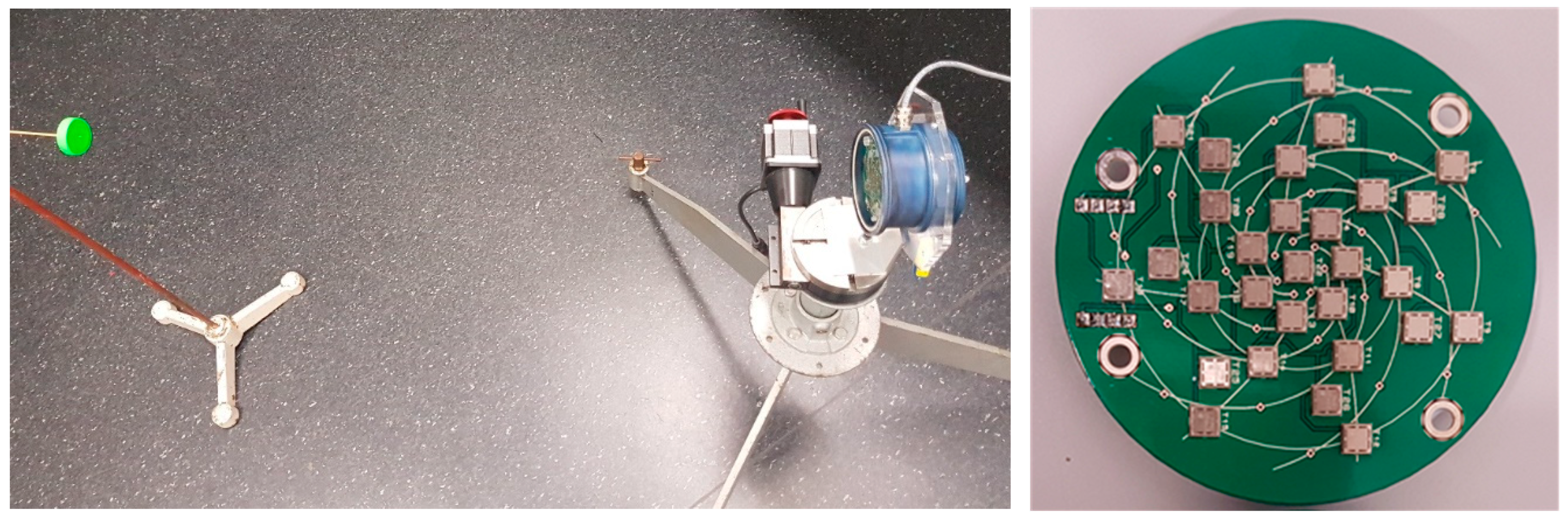
Sonar systems are similar to the new ultrasonic pasture meter in transmitting a short pulse and receiving echoes which are interpreted in terms of known types of targets [49]. A common method for calibrating sonar systems is to use a small solid sphere as a reflecting target [50]. However, the use here of a 20–35 kHz linear FM chirp signal, which has a range resolution of c/(2Δf) = 11 mm [51], means that echoes from the full sphere diameter were not sensed at once, which is quite unlike a tonal sonar calibration. Therefore, small solid circular disks of radius a were used as calibration targets. Spherical and disk shapes are not close approximations to the shape of a pasture sward, but the purpose of the laboratory calibration was to confirm the veracity of Equation (7). The size parameter range studied was ka = 1.5−10.4, generally within the geometric scattering range. The setup is shown in Figure 1. Note that the green disk is facing the array (in the blue casing), and the apparent misalignment is due to camera perspective distortion.
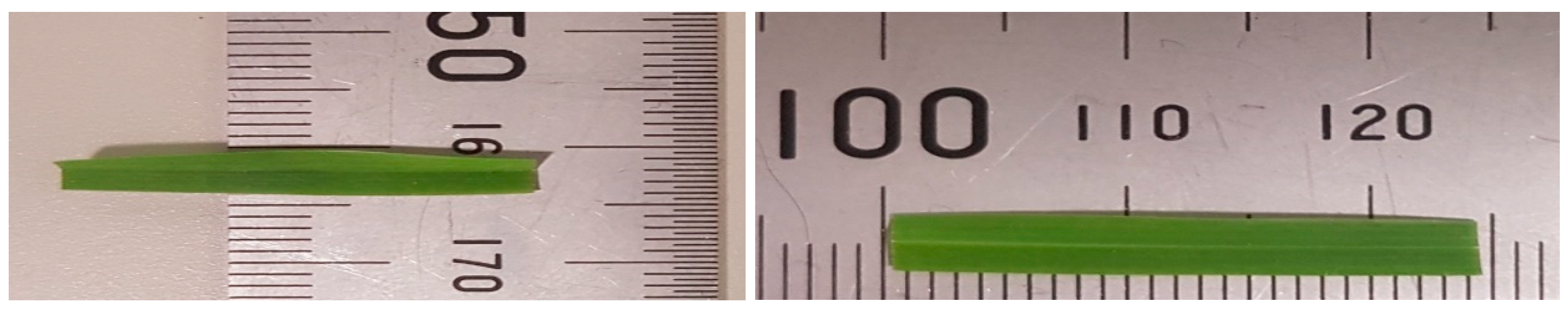
To confirm that the disks provided results which were representative of grass, measurements were also made with a segment of grass of 24.5 mm length which was trimmed from a 4.5 mm wide blade (Figure 2). Measurements were conducted of backscatter (0° incidence). The area of 24.5 × 4.5 = 110 mm2 is the same as a circular disk of radius a = 6 mm. This small length of blade was chosen so that the blade spanned an angular region over which the beam intensity was nearly constant. The blade segment was supported on a long, very fine, wire of diameter 0.32 mm. Reflection from the wire alone was undetectable.
3.1. Sensitivity
For a disk of radius a and sound normally incident:
σbs = (ka2/2)2.
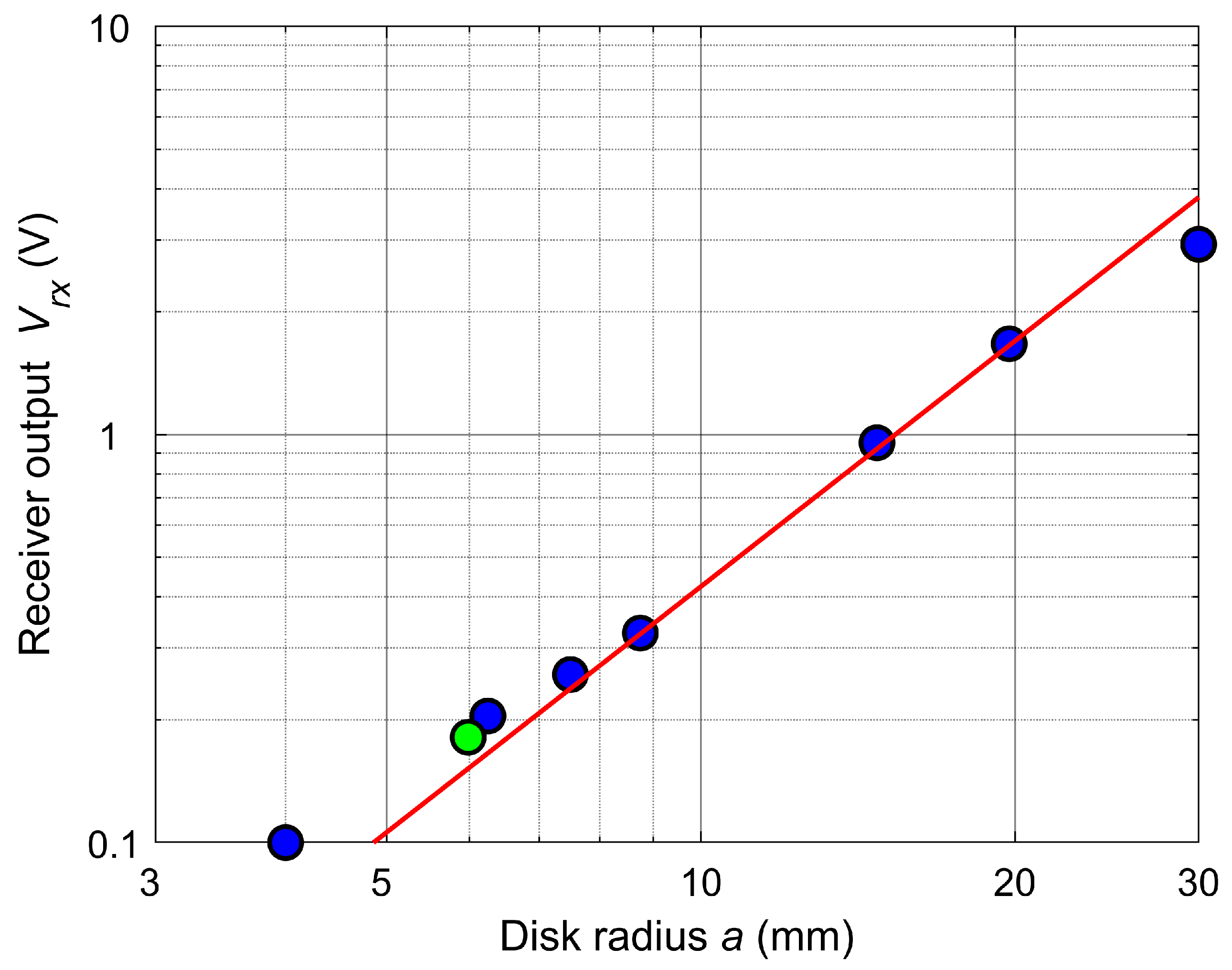
Results of measurements are shown in Figure 3 and relevant parameters in Table 1. The transmitted signal was the linear frequency-modulated (LFM) chirp [51]. The expected response, shown as a solid red line, used the specifications for the MA 40 H1S-R speaker and the SPU1410 LR5H-QB microphone, and a frequency of 24 kHz. Also shown is the response at equivalent disk radius for the blade of pasture. The grass blade segment produced a reflection close to that of a hard disk of equivalent area, indicating that ultrasound did not penetrate through the grass.
3.2. Beam Pattern
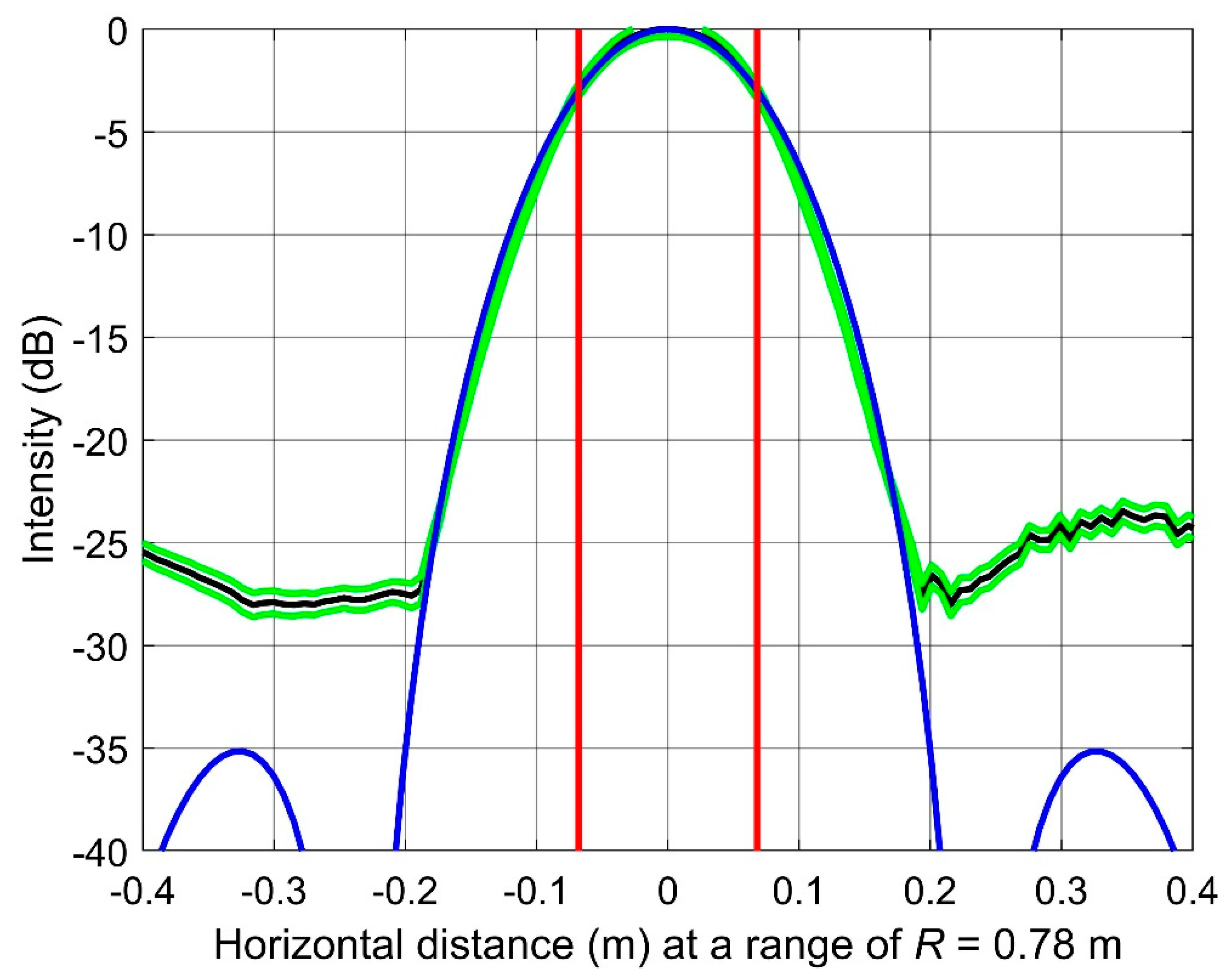
Measurements were also made to determine the beam pattern of the array. This was important, as the beam pattern determined the area of pasture that the ultrasonic sensor would sample in each transmission. In order to obtain the angular beam pattern, the ultrasonic pasture meter was mounted on a Sherline CNC Rotary Indexer. This is a rotary table using a stepping motor and gearbox producing an angular step of 0.0125°. The table and motor/gearbox can be seen beneath the pasture meter in Figure 1. Measurements were made in 0.1° steps on either side of the central direction. The distance between the pasture meter and the closest part of the target was R = 0.78 m, the approximate distance the pasture meter was mounted above the ground on the farm vehicle is described later.
The measured beam pattern for intensity is shown in Figure 4. The pattern very closely matched the Airy disk diffraction pattern over the central lobe. However, the side lobes, due to the finite number of sensors dominating from a radius of 0.2 m, projected onto the ground at a distance of 0.78 m (a beam angle of 14°). These side lobes were –20 dB, down from the –3 dB width at 68 mm radius, and are acceptable. Also shown, in green, are the measurement standard deviation around the measured pattern. The measurement error is very small. The asymmetry in the side lobe intensities is to be expected because the locations of the sensors were not symmetric.
4. Acoustic Scattering from Pasture
4.1. Theoretical Considerations
Based on the laboratory calibration, Equation (7) is a good representation of the instrument operating principles. However, a disk shape is not an adequate model for a blade of grass. A closer approximation is a finite cylinder of radius a and length L, for which [50]:
σbs = [kaL2/(4π)][2J1(kLsinθ)/(kLsinθ)]2 cos2θ.
Here, θ is the angle between the propagation direction and the normal to the cylinder axis. For 24 kHz and L = 0.14 m (i.e., a blade lying across the full beam width at half-power), σbs drops to half its maximum at θ = 1.5°. This means that the scattering is very directional. An even better scattering model would be a thin flat strip [52]. For that case, the backscatter is very sensitive to the orientation to the horizontal of the flat surface of the strip. Furthermore, blades may lie partially across the active beam area, or be partially obscured by other blades.
The net result is that modelling the detailed scattering geometry was not possible, and a statistical approach was necessary.
4.2. Field Experiment Setup
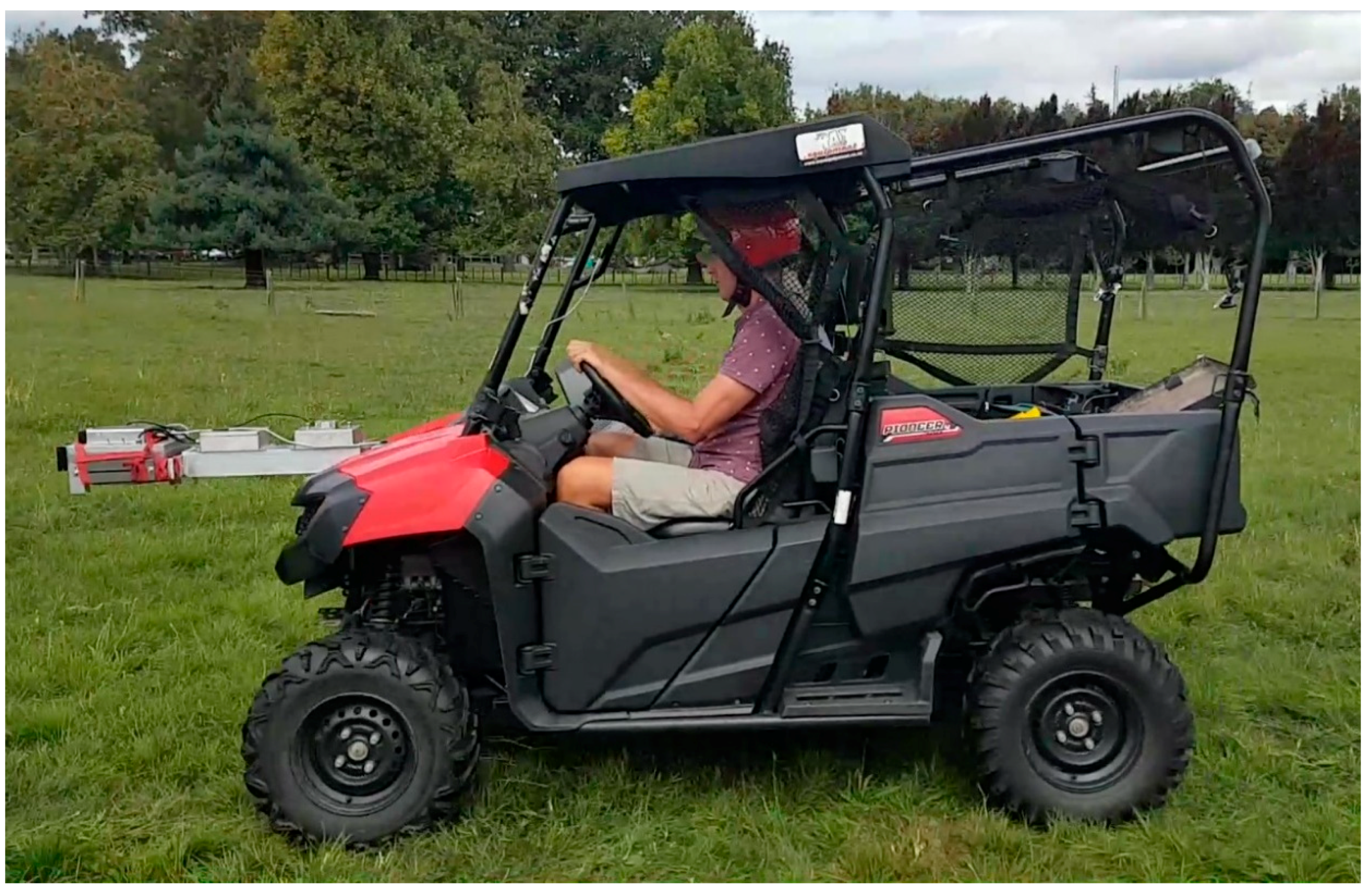
Field trials were performed to evaluate the operational performance using the hardware described in the previous section. The design goal was an instrument which will operate in real-time from a moving platform. A series of experiments were conducted with the instrument mounted on a farm vehicle, with the vehicle moving at constant speeds of 5, 10, 15, and 20 km h−1 (1.4 to 5.6 m s−1). Figure 5 shows the farm vehicle with the instrument, which is at the front of the aluminium frame. Also mounted on this frame was a much larger array, not discussed here.
The vehicle was operated at four speeds, 5, 10, 15, and 20 km h−1 (1.4, 2.8, 4.2, and 5.6 m s−1), as nearly as the driver could manage by watching the vehicle speedometer. This means that the actual platform speed varied somewhat. Three strips of pasture, or ‘transects’, were repeatedly passed over with the pasture meter. Each transect was traversed at each of the four speeds, and generally there were several ‘passes’ at each speed. Care was taken to follow the same wheel tracks at each pass over a transect, and to avoid any disturbance between the wheel tracks of the pasture being sampled. Following the vehicle operations, the pasture was cut, dried, and weighed from 0.5 × 0.5 m ‘quadrats’ along the transects.
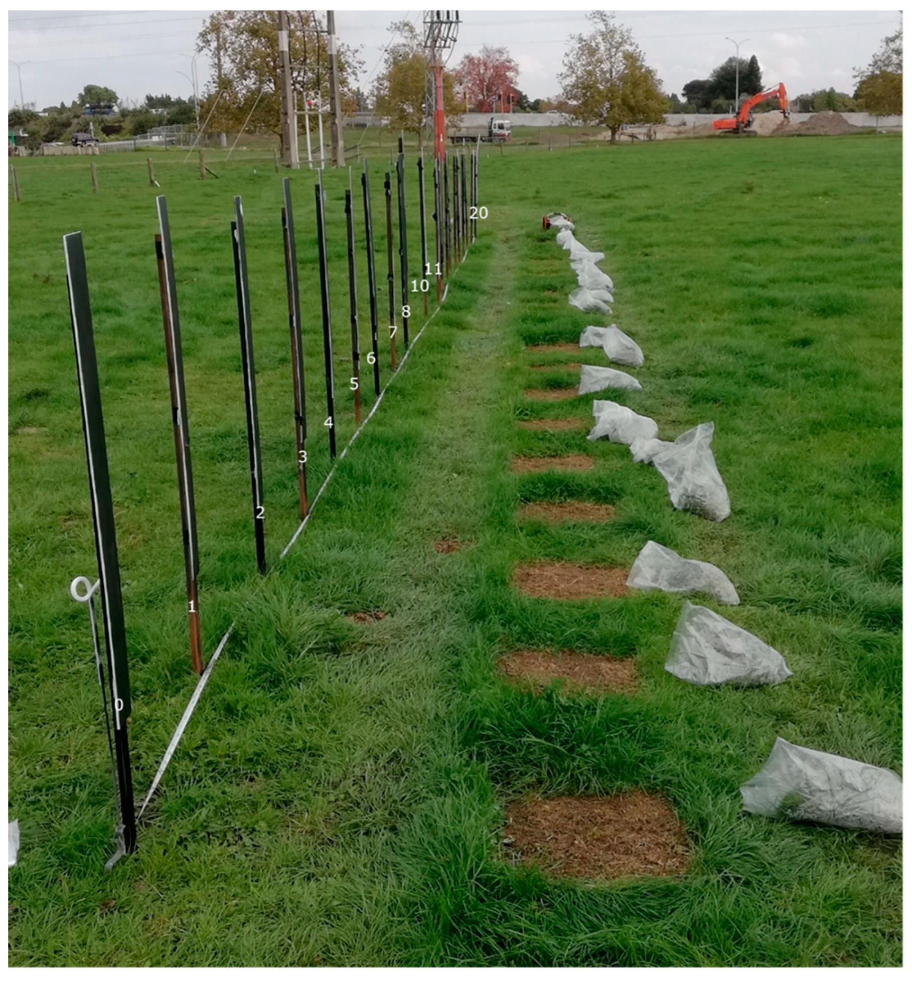
In order to compare ultrasonic measurements with the ground truth biomass obtained by cutting, a vehicle position registration scheme was required. The ultrasound profiles needed to be located within the 0.5 m cut areas, so registration to better than 0.1 m was ideally required. Smartphone and mapping grade GPS do not achieve this accuracy [53]. Using real-time differential corrections allows navigation to within one to two meters of any location depending on the service and the GPS receiver, and only under the very best conditions can 0.1 m accuracy be obtained. Therefore, an alternative registration method was devised. This involved setting posts at intervals along the edge of a transect and using an infrared sensor to detect each post as the vehicle passed by. The ultrasonic and infrared signals were simultaneously sampled. This allowed the farm bike speed to be measured and the location of each ultrasonic transmission to be estimated. The method was under review during the field experiments, because some of the posts were not registered by the infrared sensor in bright sunlight. This meant that a different scheme was used for each transect. Transect 1 had 21 posts at 1 m intervals, with the overall transect length being 20 m. Detection of a post caused the transmission of three ultrasonic pulses, at 50 ms intervals, except for the first post, for which there were six ultrasonic pulses transmitted at 50 ms intervals. Post number 9 was omitted, so that the gap could be an extra reference point. Biomass quadrats were centered on each post position, as shown in Figure 6.
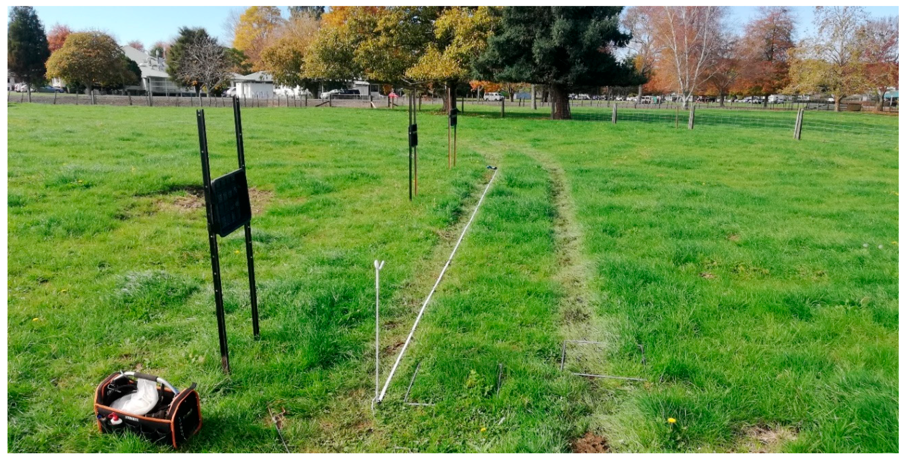
For Transects 2 and 3, the pasture meter produced pulses at 50 ms intervals but freely running and not aligned to the posts. Transect 2 had 0.5 m-wide reflectors extending from 0 to 0.5 m, from 4.5 to 5 m, and from 9.5 to 10 m, and reflecting individual posts at 6, 6.5, 7, 7.5, 8, 8.5, and 9 m. Transect 3 had only three 0.5 m-wide reflectors, at 0 to 0.5 m, 6.05 to 6.55 m, and 9.55 to 10.05 m, as shown in Figure 7. For Transects 2 and 3, biomass was measured every 0.5 m, starting at 0 to 0.5 m, giving 20 biomass measurements over the transect length of 10 m. Table 2 and Table 3 summarize the setup parameters.
4.3. Ultrasonic Profiles
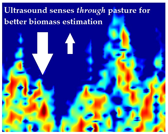
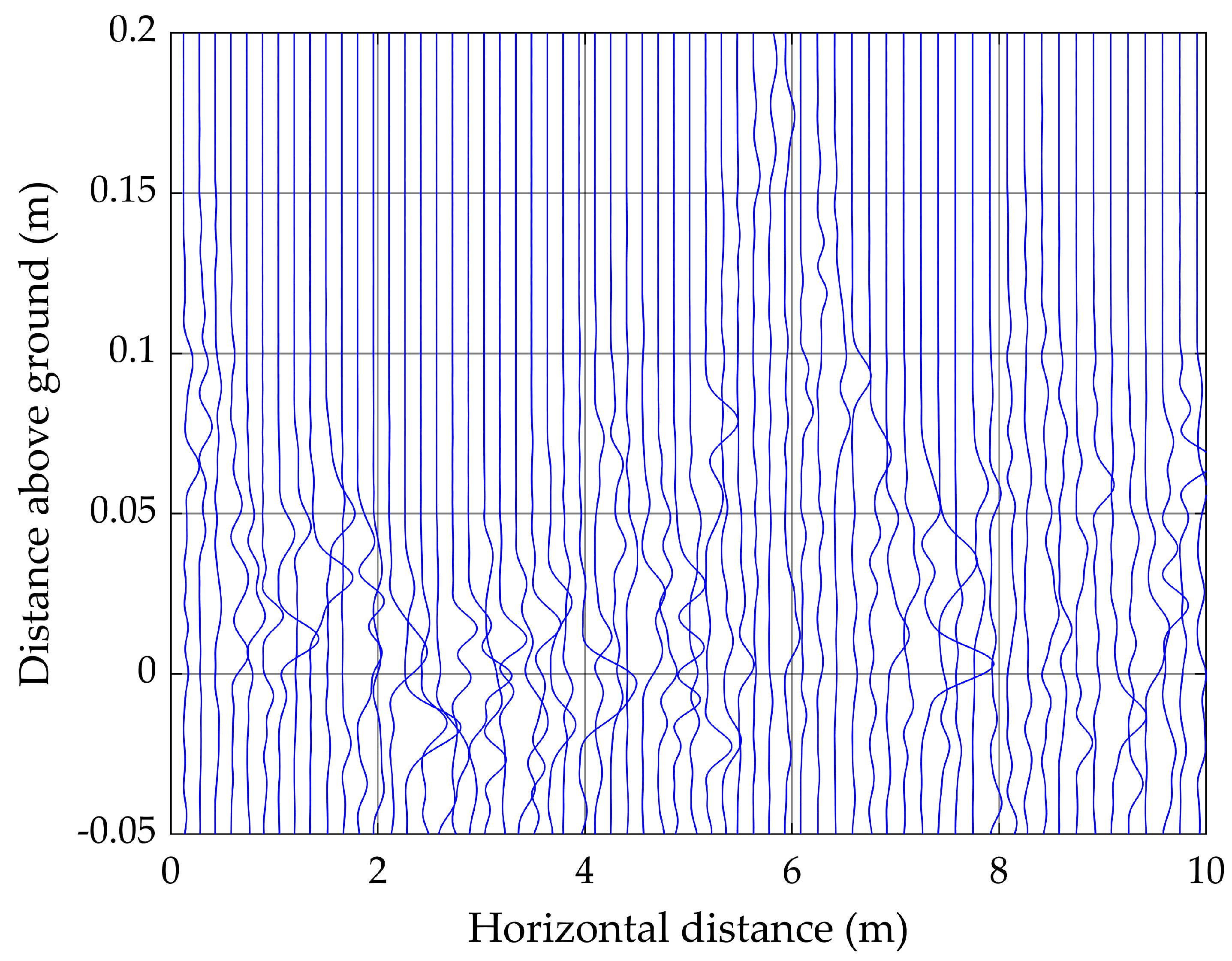
Figure 8 shows a waterfall display of all the reflectance profiles from Pass 4 at 10 km h−1 from Transect 3. There are features of this plot common to all speeds and transects. Firstly, the top of the pasture is relatively easily seen as the region above which the reflectivity does not vary. A simple thresholding scheme allows this point to be estimated. Secondly, there are frequently reflectance peaks near the expected ground (vertical distance 0 m in the figure), but not always so. In practice, reflectivity is windowed in a region around the expected range to the ground and the position of the maximum within that window taken to be the ground position. Thirdly, all profiles exhibit a relatively small number of well-defined peaks, each of which has similar properties to the expected chirp response to a point reflector [51]. This suggests that a few individual blades of grass are contributing to the reflectance for each profile. The correlation between peak positions in adjacent profiles is not high, so the dominant grass blades do not clearly extend across profiles. Fourthly, there are reflections at ranges greater than the instrument-to-ground range, labelled on this plot as being ‘below ground’. These arise from multiple reflections.
4.4. Reflecting Objects
The peaks above a given threshold of 0.25 V2 were identified using the CLEAN algorithm [54]. In this algorithm, the peak was found and then removed, assuming the shape predicted from the chirp response. The peak in the modified, ‘cleaned’ profile was then found and the process repeated. The CLEAN algorithm enables an enhanced vertical resolution. An example is given in Figure 9. Overlapping peaks are also evident.
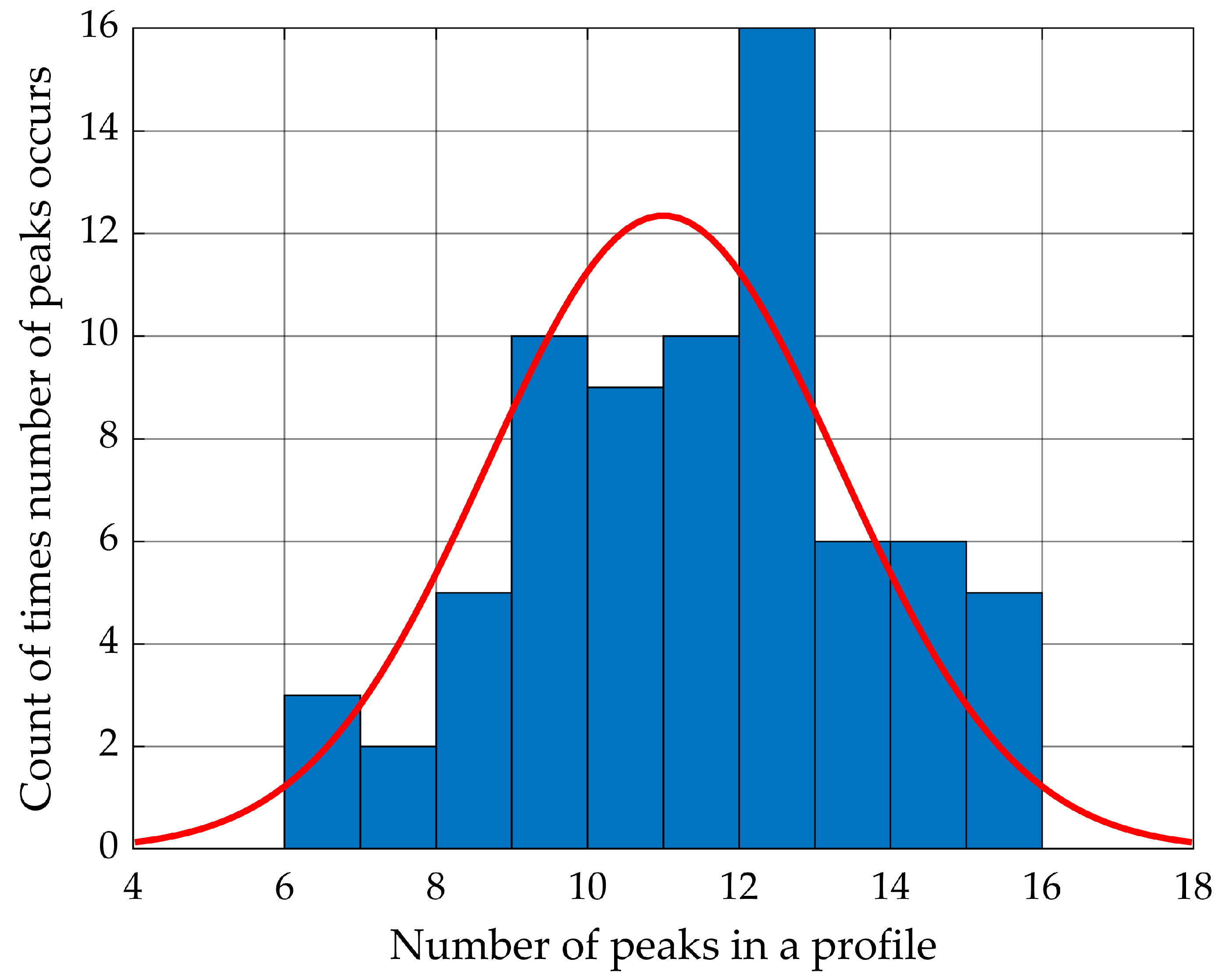
A sward height of around 0.1 m corresponds to a biomass of around 0.2 kg m−2 (see Figure 13 below), or a bulk density of around ρ = 2 kg m−3. Taking the 3 dB width of the ultrasonic beam as 0.14 m, the volume sampled was around Vs = 1.5 x 10⁻³ m3, so the dry mass within the beam was around ρVs = 3 x 10⁻³ kg. Figure 10 shows the number distribution per profile of peaks exceeding the 0.25 V2 threshold, with an average of 11 blades sensed in each profile. The dry mass per sensed blade would therefore be around 3 x 10⁻⁴ kg. DM is typically 35%, giving a blade density of 350 kg m−3, so an average sensed blade volume would be 8 x 10⁻⁷ m3. Assuming each grass blade is of width 5 mm and lies across this volume, the thickness of a grass blade would be around 1 mm. While this calculation is very crude, this estimated blade thickness is far too high. The conclusion is that not all blades were sensed, because of the variation in blade orientation.
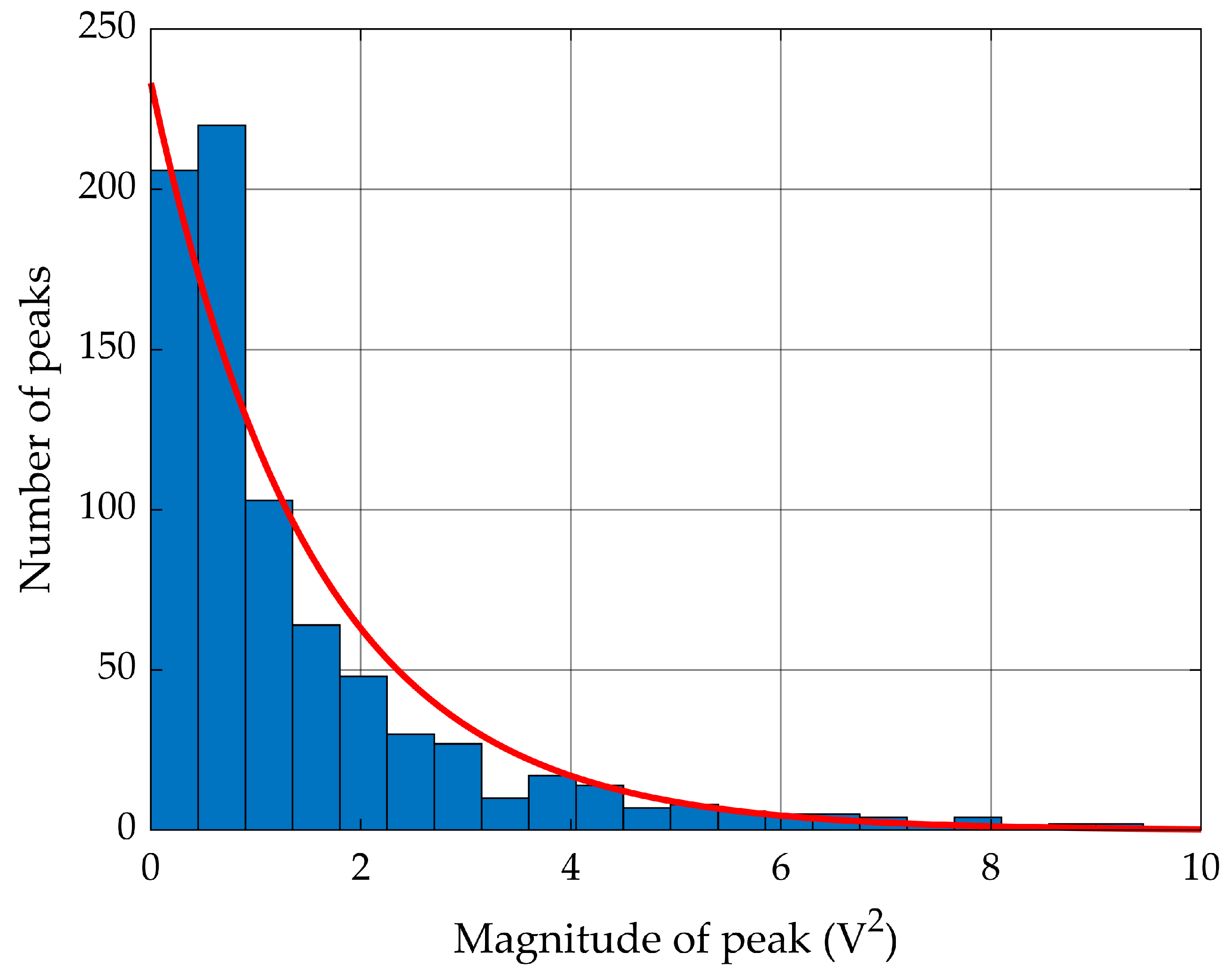
The probability distribution of the magnitude of the peaks, shown in Figure 11, reflects the probability distribution of the blade orientations and the variation in blade size. It is beyond the scope of the present work to attempt to separate these two effects. The mean magnitude of a peak is 1.5 V2. Most of the variability in numbers of peaks is in the smaller magnitude peaks, meaning that the discrete random nature of the number of blades of grass reflecting from within the sensitive volume of this instrument is only a few percent.
4.5. Multiple Scattering
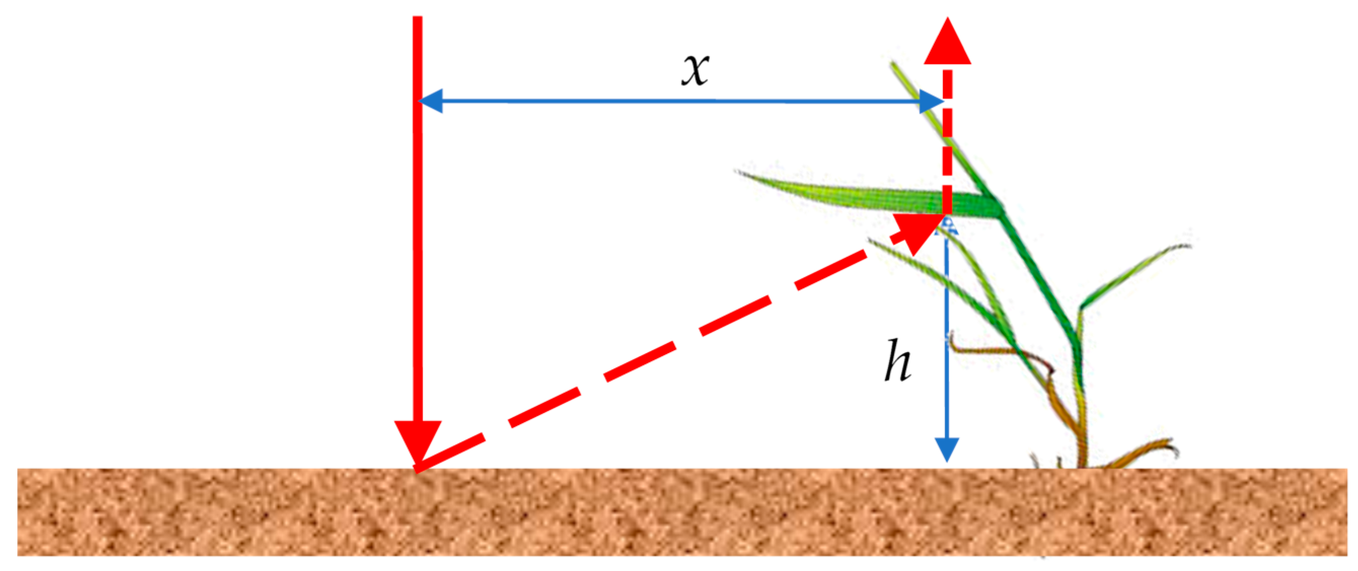
The profiles shown in Figure 8 and Figure 9 show ‘distance above ground’ as being negative for some reflectance peaks. These peaks occurred from ranges further than the distance from the instrument to the ground and arose from secondary scattering. Figure 12 shows the geometry. The path could either be a ground reflection followed by a pasture reflection (as shown) or a pasture reflection followed by a ground reflection. The extra path length beyond the instrument-ground distance was (x2 + h2)1/2, but since the distance to the reflector was half the path length, the apparent ‘below ground’ distance was (x2 + h2)1/2/2. For a sward height of 0.2 m and a 3 dB beam half-width of 0.07 m, the maximum extra distance for secondary scattering would be 0.11 m. This is consistent with what is shown in Figure 9.
The fact that secondary scattering is always seen as discrete scattering events means that there is always penetration of the ultrasound to the ground, although the ground may not be the dominant scatterer. The small number of physically small scattering elements from the pasture means that secondary scattering from a grass blade onto another grass blade and then onto the receivers was insignificant.
5. Relationship between Biomass and Back-scattered Ultrasonic Power
5.1. Biomass and Reflectance
The biomass is:
where ρ is the bulk density of B, H is the depth of the pasture, and height h is measured upward from the ground. The bulk density includes the empty space between grass blades.
B = ∫dB = ∫ρdh,
Assume that at height h there are nv(h) identical grass blades per unit volume, each having mass m(h) and back-scattering cross section σbs(h). In the height interval h to h + dh, the biomass is:
dB = mnVdh.
The backward scattered acoustic power, dP, from the same volume is:
where Pi is the power incident on the area at depth h. Combining Equations (12) and (13),
where β will be called the “blade areal density”. Like B, β is a mass per unit area.
dP = PiσbsnVdh,
dB = (mi/σbs)dP/Pi = β(h) dPi/Pi,
5.2. Height Variation within the Pasture Layer
Both the blade areal density and the back-scattered acoustic power may be expected to vary with depth within the pasture layer. Expanding the blade areal density as a polynomial in h,
giving:
where cn = bn/Pi and:
β(h) = Σ hnbn,
B = Σ bn ∫hndP/Pi = Σ cnRn,
Rn = ∫hndP.
The Rn are measures of the shape of the reflectivity profile. For example,
and:
are the power-weighted mean height and height variance within the pasture layer. R3 is a measure of skewness and R4 a measure of kurtosis.
μh = ∫hdP/∫dP,
σh2 = ∫(h-μh)2dP/∫dP = R2/R0-μh2,
Equation (16) is a calibration equation which estimates biomass B for each ultrasonic profile using the Rn derived from the profile reflectivity and using the constant calibration coefficients cn. It predicts that B = 0 when H = 0, in accordance with expectations, but in contrast to calibration equations for other pasture biomass instruments, such as the Rising Plate meter or C-Dax. Underpinning this approximation is the major assumption that β(h) has a constant shape for all sward heights and varieties. Essentially, this is assuming that if the mass m(h) of a blade in a layer increases, then the back-scattering cross section σbs(h) increases proportionally. While not physically unreasonable, this assumption can only be tested through field investigations, in which the biomass is measured by cutting, drying, and weighing. Note that this assumption does not restrict the shape of the overall biomass profile.
5.3. Field Calibration Methodology
Equation (16) provides a basis for field calibration, in which biomass Bq is measured via cutting, drying, and weighing at a number of quadrats q = 1, 2, …, Q together with ultrasonic pasture meter profiles providing backscattered power dPj,q at height intervals j in each quadrat. The regressors Rn,q are obtained from these measurements and a multiple linear regression performed to estimate the coefficients cn.
If these calibrations are performed over a number of pasture sites, seasons, and varieties, then the assumption that the cn is constant can be checked, and also how well the overall model explains variance in measured B.
5.4. Relationship to Other Methods
From equations (13) and (17):
providing the term in brackets is constant throughout the pasture layer. This is equivalent to the approximation made by the ultrasonic sward and the C-Dax, for which it is assumed that the biomass is proportional to sward height H. From our field data (see below) we can estimate the residuals between our profile approximation (16) and the depth-only approximation (20).
R0 = ∫dP = (Piσbsρh)H,
6. Field Results
The field data are extensive and only a subset of results will be discussed here. A following publication will contain an exhaustive presentation and discussion of all transect data, as well as data from a non-moving platform.
6.1. Biomass Versus Sward Height
The sward height H can be estimated solely from the ultrasonic profile based on the position of a reflectance peak in the vicinity of the expected ground location. This allows for vertical movement of the farm vehicle due to its suspension. Biomass B was measured by cutting the pasture, drying the sample, and weighing it, and taking into account the area cut.
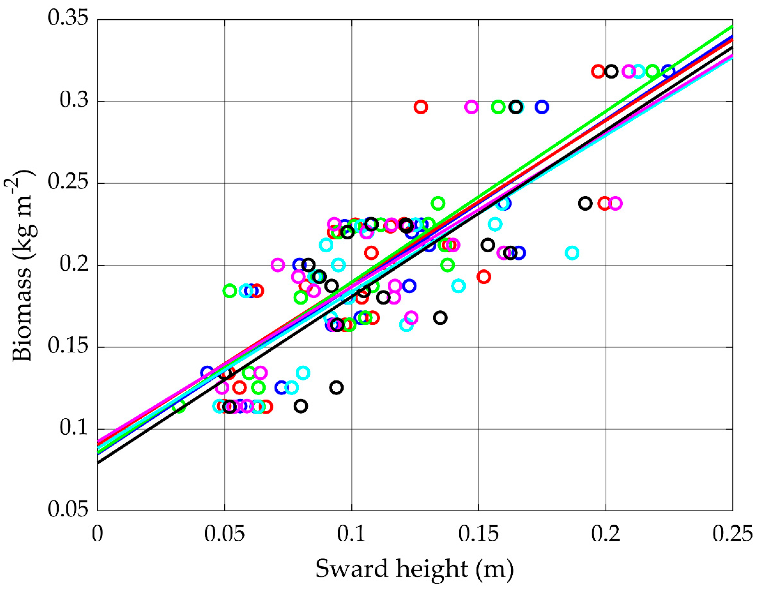
From Table 2, Transect 3 provided six passes over the same pasture at 10 km h−1. The results of linear regressions of the following form:
are shown in Figure 13. The six colors represent the six different passes. The coefficient of determination, R2, varies from 0.61 to 0.75, with a mean value of 0.66. Over all passes for this transect, at all speeds, the slope is μρ = 0.97 ± 0.05 kg m−3 and the intercept is B0 = 0.088 ± 0.005 kg m−2. In common with the methods used by the C-Dax, ultrasonic sward stick, and other biomass estimations based on sward height, this regression model is non-physical because it predicts a non-zero biomass for zero sward height.
B = B0+μρH,
6.2. Biomass Estimation Using the Reflectivity Profile
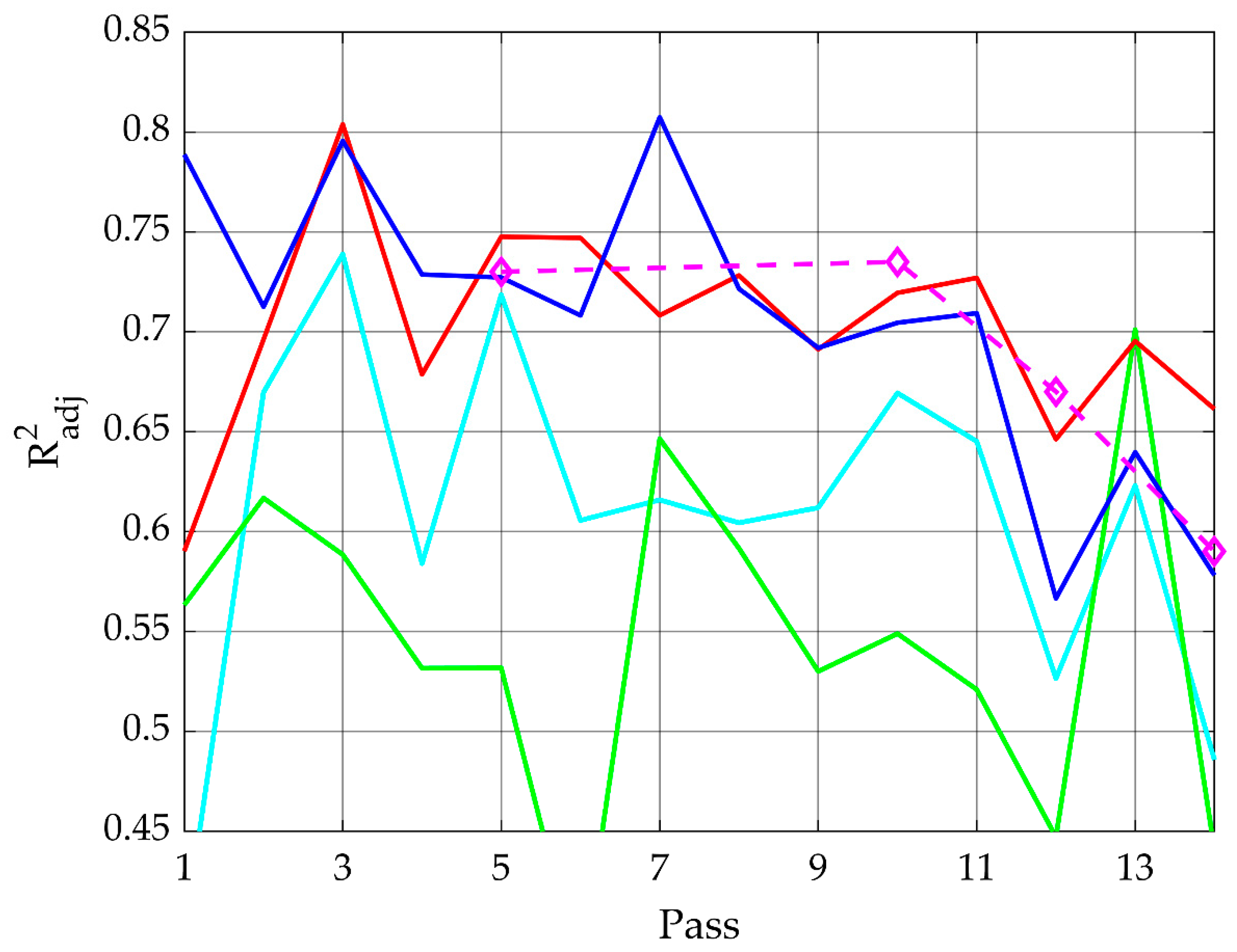
Regression models were evaluated with regressors H, R0, R1, R2, and R3 in various combinations. These models did not have a constant intercept, except for the model in equation (21), so they predicted that B → 0 as H → 0, which is physically reasonable. Results from the four models listed in Table 4 are shown here.
Model 1 was simply dependence on sward height expressed by Equation (21). Model 2 was the N = 2 model from Equation (16). Models 3 and 4 used regressor H instead of R0 for the reason that it was found that much higher values of R2 are obtained. Figure 14 shows the adjusted R2 values obtained for the four models and for each of the 14 passes from Transect 3. The adjusted R2 is related to R2 via the following:
Radj2 = 1-(1-R2)(Q-1)/(Q-1-N).
Adjusted R2 allows for the inflation of R2, which occurs as more regressors are added. As can be seen, the use of R0 gives a poor estimation of B. The two models, 3 and 4, which included profile information performed better than the depth-only model 1 across all passes at all speeds. Pass 1 exhibited some problems because of difficulty in registration with the reflectors. There was an indication that estimation of biomass at 20 km h−1 was slightly worse than at other speeds.
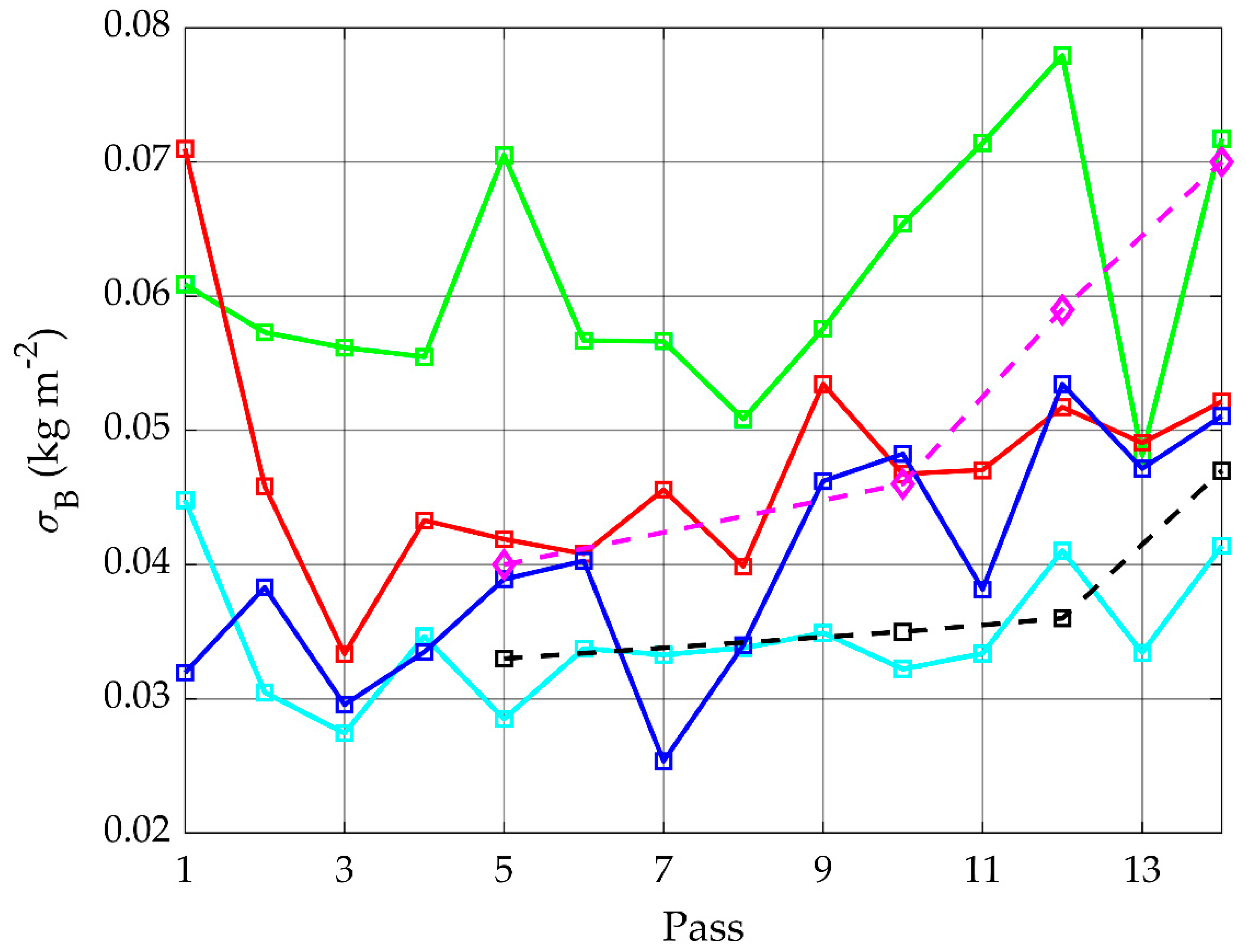
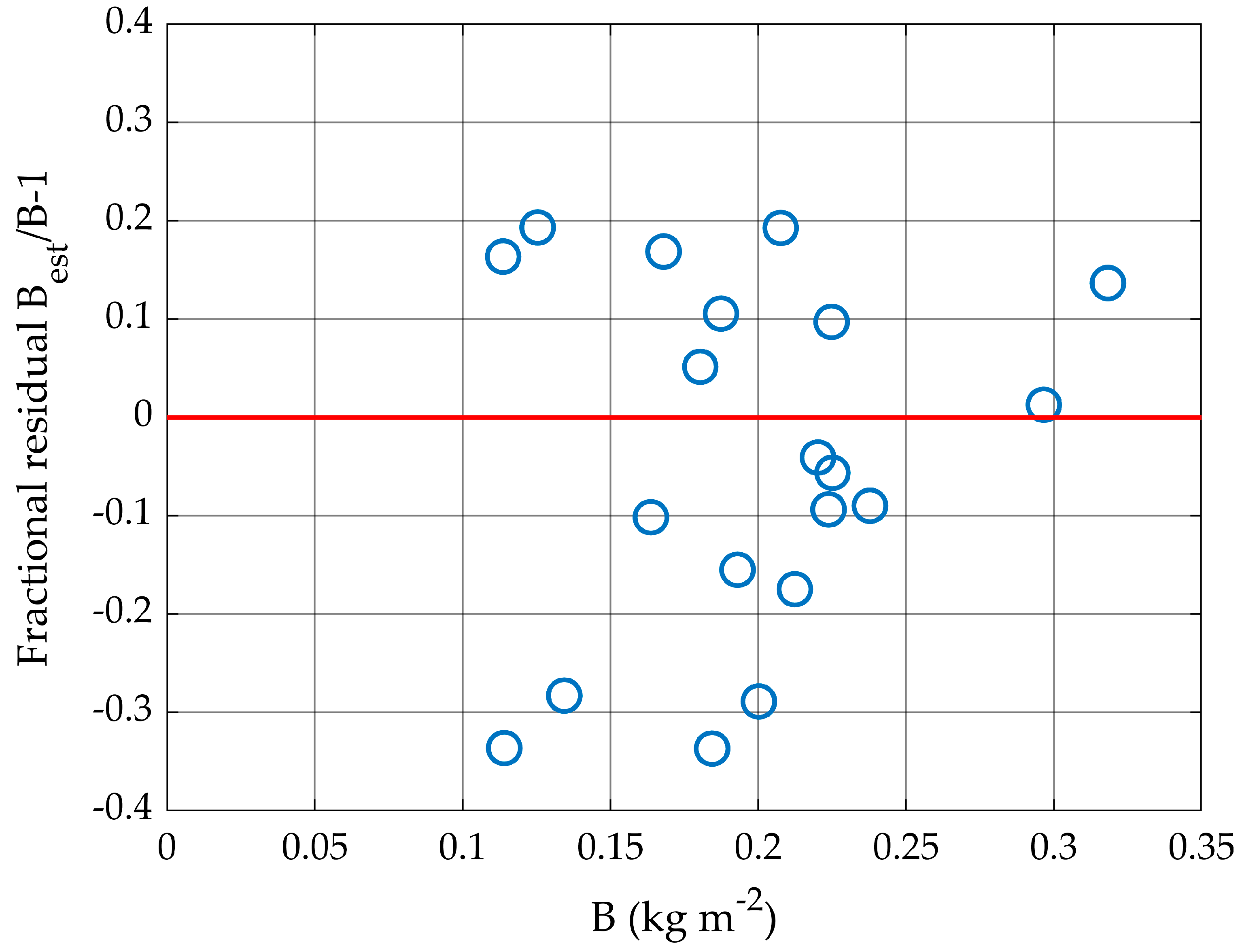
More important than R2 is the estimation error, σB, for biomass based on these regressions. Figure 15 shows this estimation error for the four models and 14 passes. Excluding Pass 1, the mean estimation error for the four models was 340, 610, 460, and 400 kg m−2. The best performance was by the sward height model, B = B0 + μρH, and then the three-regressor model B = c0H + c1R1 + c2R2. Figure 16 shows residuals at one of the best passes, Pass 3, for the model B = c0H + c1R1. Residuals did not show a well-defined increase with biomass B or sward height H, so are probably more closely related to model error rather than measurement error.
6.3. Model Resilience
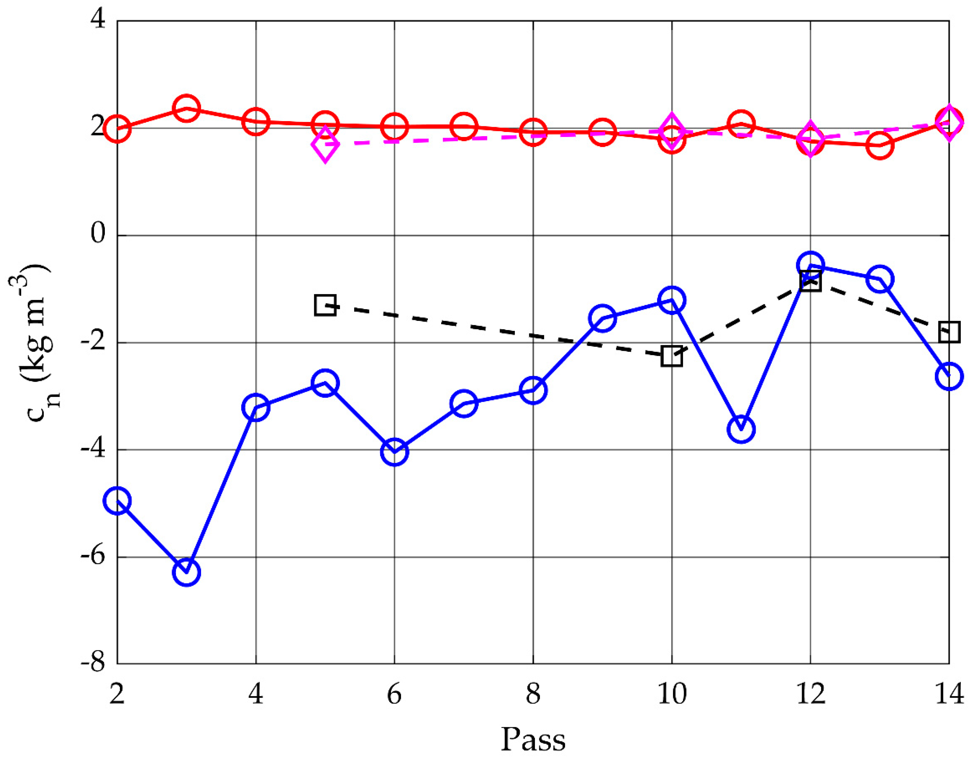
From the data shown in Figure 15, the estimation error varied around 12% over Passes 2 to 14 for models B = B0 + μρH and B = c0H + c1R1, and around 21% for model B = c0H + c1R1 + c2R2. The variation of the two fitted coefficients, c0 and c1, for B = c0H+c1R1 are shown in Figure 17. The first coefficient varied little over Passes 2 to 14. The second coefficient appeared to increase slightly with vehicle speed, but this is as likely to be a registration outcome as a genuine speed dependence.
7. Discussion and Conclusions
Biomass is a crucial parameter in optimally managing the farming of grazing animals. Direct biomass measurement, via cutting and weighing, is destructive and time-consuming, as well as potentially giving results not representative of the larger pasture area. Consequently, a number of indirect methods have arisen. Sensors on satellite platforms have the advantages of providing data with a large areal coverage, at modest cost, and reasonable repetition rates. Furthermore, the use of wavelengths over a wide spectral range can provide not just biomass information, but also forage quality information. Nevertheless, farmers also may prefer a more immediate hands-on estimation method, which they can deploy during the normal course of their farm operations under any weather conditions. Of these proximal methods, the most convenient provide biomass estimation from a moving farm vehicle. However, such methods generally correlate an estimate of the pasture height with measured biomass, and the correlations are not robust across pasture species and seasons.
A new low-frequency ultrasound instrument was described, which has the capability of both sensing the depth of the pasture and penetrating through the pasture to the ground. The instrument achieves this by using a range of frequencies in an FM chirp, which also provides for high vertical spatial resolution of 11 mm. By penetrating through the pasture, it is possible to record the reflectance profile, which is related to pasture or biomass density.
The calibration of the new instrument was found to agree closely with theoretical expectations based on sensor specifications and the arrangement of sensors in spiral arrays. The ultrasonic beam pattern provided a –3 dB footprint diameter of 0.14 m, which is sufficiently small to avoid gross variations in biomass across the diameter, while being sufficiently large that statistics of small numbers of blades of grass being sampled is not a problem. Estimates of scattering strength agree with observations, lending confidence to the understanding of the principles upon which the methodology is based.
A model was developed for the scattering of ultrasound by pasture. This model makes a connection between observations of reflectance and the biomass in the field of view. From this connection, a number of suitable regressors were suggested between ultrasonic observables and biomass. Field studies conducted at vehicle speeds of 5 to 20 km h−1, together with direct biomass measurements, allowed a number of regression models to be evaluated. It was found that the best models included both pasture height and at least one measure of reflectance variation within the pasture layer. By including variation within the pasture layer, biomass estimation was significantly improved. The coefficient of variation, R2, if pasture height alone was used, was in the range 0.6 to 0.7 in these studies, compared with a range of 0.7 to 0.8 if profile information was included. The model also appeared to be resilient in that the regression coefficients were stable with vehicle speed and with a range of pasture covers.
The integrated ultrasonic reflectance, which provides extra information, depends on the amplitude of reflected ultrasound from each pasture blade within the sampled volume of pasture. A crude calculation, based on numbers of signal peaks from within the pasture canopy, suggested variations in blade orientation cause a substantial number of blades to return low amplitudes. This means that the regressors based on reflectance are in practice averages over the probability distribution of blade orientation. Nevertheless, this averaging appears to be robust, since multiple passes over the same pasture gave similar results in spite of the disturbance caused by the farm vehicle having passed above the pasture.
Some of the unexplained variance (or the fact that R2 is less than 1) was undoubtedly due to remaining difficulties in registering the location of ultrasonic profiles with the location of cut quadrats used for reference biomass measurements. A further contribution to unexplained variance will be from pasture moisture variations, although this is thought to be a small influence since multiple passes over pasture on different days and times of day showed undetectable regression variations.
The instrument is small, low-power, and easy to use, and has the potential to be a readily accessible and useful addition to precision agriculture.
8. Patents
S. Bradley, M. Legg, Systems, apparatus and methods for vegetation measurement, No.753949, Nationality: New Zealand, Gallagher Group Limited. (28 May 2019).
S. Bradley, M. Legg, Vegetation measurement apparatus, systems, and methods, No.2019201425, Nationality: Australia, Gallagher Group Limited (28 Feb. 2019).
Author Contributions
Conceptualization, S.B.; methodology, S.B.; software, M.L. and S.B.; validation, M.L. and S.B.; formal analysis, M.L. and S.B.; investigation, M.L. and S.B.; resources, S.B.; data curation, M.L. and S.B.; writing—original draft preparation, S.B.; writing—review and editing, M.L. and S.B.; visualization, S.B.; supervision, S.B.; project administration, S.B.; funding acquisition, S.B.
Funding
This work was supported by a grant from the New Zealand Ministry of Business, Innovation and Employment (MBIE), and by co-funding from Gallagher Group Ltd.
Acknowledgments
The authors are grateful for the collegial interactions with colleagues at Gallagher and from AgResearch. The bulk of this work was completed while S.B. was a professor at the Physics Department, University of Auckland, Private Bag 92019, Auckland, New Zealand.
Conflicts of Interest
The authors declare no conflict of interest.
References
- Allen, V.G.; Batello, C.; Berretta, E.J.; Hodgson, J.; Kothmann, M.; Li, X.; McIvor, J.; Milne, J.; Morris, C.; Peeters, A. An international terminology for grazing lands and grazing animals. Grass Forage Sci. 2011, 66, 2–28. [Google Scholar] [CrossRef]
- Beukes, P.; McCarthy, S.; Wims, C.; Gregorini, P.; Romera, A. Regular estimates of herbage mass can improve profitability of pasture-based dairy systems. Anim. Prod. Sci. 2019, 59, 359–367. [Google Scholar] [CrossRef]
- Gebremedhin, A.; Badenhorst, P.; Wang, J.; Spangenberg, G.; Smith, K. Prospects for measurement of dry matter yield in forage breeding programs using sensor technologies. Agronomy 2019, 9, 65. [Google Scholar] [CrossRef]
- Earle, D.; McGowan, A. Evaluation and calibration of an automated rising plate meter for estimating dry matter yield of pasture. Austr. J. Experim. Agric. 1979, 19, 337–343. [Google Scholar] [CrossRef]
- Nakagami, K.; Itano, S. Improving pooled calibration of a rising-plate meter for estimating herbage mass over a season in cool-season grass pasture. Grass Forage Sci. 2014, 69, 717–723. [Google Scholar] [CrossRef]
- Angelone, A.; Toledo, J.M.; Burns, J.C. Herbage measurement insitu by electronics.1. The multiple-probe-type capacitance meter: a brief review. Grass Forage Sci. 1980, 35, 25–33. [Google Scholar] [CrossRef]
- Serrano, J.M.; Peça, J.O.; Marques da Silva, J.; Shahidian, S. Calibration of a capacitance probe for measurement and mapping of dry matter yield in Mediterranean pastures. Precis. Agric. 2011, 12, 860–875. [Google Scholar] [CrossRef]
- Murphy, W.; Silman, J.; Barreto, A.M. A comparison of quadrat, capacitance meter, HFRO sward stick, and rising plate for estimating herbage mass in a smooth-stalked, meadow grass-dominant white clover sward. Grass Forage Sci. 1995, 50, 452–455. [Google Scholar] [CrossRef]
- Clarke, D.; Litherland, A.; Mata, G.; Burling-Claridge, R. Pasture monitoring from space. In Proceedings of the South Island Dairy Event (SIDE) Conference, Lincoln, UK, 24–29 June 2009; pp. 26–28. [Google Scholar]
- Hunt, C.L.; Jones, C.S.; Hickey, M.; Hatier, J.H.B. Estimation in the field of individual perennial ryegrass plant position and dry matter production using a custom-made high-throughput image analysis tool. Crop Sci. 2015, 55, 2910–2917. [Google Scholar] [CrossRef]
- L´opez-D´ıaz, J.; Roca-Fern´andez, A.; Gonz´alezRodr´ıguez, A. Measuring herbage mass by non-destructive methods: A review. J. Agric. Sci. Technol. JAST 2011, 1, 303–314. [Google Scholar]
- Chao, Z.; Liu, N.; Zhang, P.; Ying, T.; Song, K. Estimation methods developing with remote sensing information for energy crop biomass: A comparative review. Biomass Bioenergy 2019, 122, 414–425. [Google Scholar] [CrossRef]
- Xue, J.; Su, B. Significant remote sensing vegetation indices: A review of developments and applications. J. Sens. 2017, 1–17. [Google Scholar] [CrossRef]
- Genever, L. Developing Grazing Systems for Beef Producers: A review of grassland tools. ADAS UK Ltd. 2016. Available online: http://beefandlamb.ahdb.org.uk/wp-content/uploads/2017/11/20160222_Grass-from-beef_tool-review_V4.pdf (accessed on 22 October 2019).
- Andersson, K.; Trotter, M.; Robson, A.; Schneider, D.; Frizell, L.; Saint, A.; Lamb, D.; Blore, C. Estimating pasture biomass with active optical sensors. Adv. Anim. Biosci. 2017, 8, 754–757. [Google Scholar] [CrossRef]
- Hanna, M.; Steyn-Ross, D.; Steyn-Ross, M. Estimating biomass for New Zealand pasture using optical remote sensing techniques. Geocart. Int. 1999, 14, 89–94. [Google Scholar] [CrossRef]
- Gu, Y.; Wylie, B.K.; Howard, D.M.; Phuyal, K.P.; Ji, L. NDVI saturation adjustment: A new approach for improving cropland performance estimates in the Greater Platte River Basin, USA. Ecol. Indic. 2013, 30, 1–6. [Google Scholar] [CrossRef]
- Wachendorf, M.; Fricke, T.; Möckel, T. Remote sensing as a tool to assess botanical composition, structure, quantity and quality of temperate grasslands. Grass Forage Sci. 2018, 73, 1–14. [Google Scholar] [CrossRef]
- Cao, Z.; Cheng, T.; Ma, X.; Tian, Y.; Zhu, Y.; Yao, X.; Chen, Q.; Liu, S.; Guo, Z.; Zhen, Q.; et al. A new three-band spectral index for mitigating the saturation in the estimation of leaf area index in wheat. Int. J. Remote Sens. 2017, 38, 3865–3885. [Google Scholar] [CrossRef]
- Serrano, J.; Shahidian, S.; Marques da Silva, J. Calibration of Grassmaster II to estimate green and dry matter yield in Mediterranean pastures: Effect of pasture moisture content. Crop Pasture Sci. 2016, 67, 780–791. [Google Scholar] [CrossRef]
- Serrano, J.M.; Shahidian, S.; Da Silva, J.R.M. Monitoring pasture variability: optical OptRxR crop sensor versus Grassmaster II capacitance probe. Environ. Monit. Assess. 2016, 188, 117. [Google Scholar] [CrossRef]
- Schulze-Brüninghoff, D.; Hensgen, F.; Wachendorf, M.; Astor, T. Methods for LiDAR-based estimation of extensive grassland biomass. Comput. Electron. Agric. 2019, 156, 693–699. [Google Scholar] [CrossRef]
- Pasqualotto, N.; Delegido, J.; Van Wittenberghe, S.; Rinaldi, M.; Moreno, J. Multi-Crop Green LAI Estimation with a New Simple Sentinel-2 LAI Index (SeLI). Sensors 2019, 19, 904. [Google Scholar] [CrossRef]
- Atzberger, C.; Darvishzadeh, R.; Immitzer, M.; Schlerf, M.; Skidmore, A.; le Maire, G. Comparative analysis of different retrieval methods for mapping grassland leaf area index using airborne imaging spectroscopy. Int. J. Appl. Earth Observ. Geoinf. 2015, 43, 19–31. [Google Scholar] [CrossRef] [Green Version]
- Berger, K.; Atzberger, C.; Danner, M.; D’Urso, G.; Mauser, W.; Vuolo, F.; Hank, T. Evaluation of the PROSAIL model capabilities for future hyperspectral model environments: a review study. Remote Sens. 2018, 10, 85. [Google Scholar] [CrossRef]
- Barthram, G. Experimental Techniques: The HFRO Sward Stick; Technical report; The Hill Farming Research Organization: Midlothian, UK, 1985. [Google Scholar]
- Hutchings, N.; Phillips, A.; Dobson, R. An ultrasonic rangefinder for measuring the undisturbed surface height of continuously grazed grass swards. Grass Forage Sci. 1990, 45, 119–127. [Google Scholar] [CrossRef]
- Hutchings, N. Spatial heterogeneity and other sources of variance in sward height as measured by the sonic and HFRO sward sticks. Grass Forage Sci. 1991, 46, 277–282. [Google Scholar] [CrossRef]
- Hutchings, N. Factors affecting sonic sward stick measurements: the effect of different leaf characteristics and the area of sward sampled. Grass Forage Sci. 1992, 47, 153–160. [Google Scholar] [CrossRef]
- Fricke, T.; Richter, F.; Wachendorf, M. Assessment of forage mass from grassland swards by height measurement using an ultrasonic sensor. Comput. Electron. Agric. 2011, 79, 142–152. [Google Scholar] [CrossRef]
- Zhou, Z.; Parsons, D. Estimation of yield and height of legume-grass swards with remote sensing in northern Sweden. In Sustainable Meat and Milk Production from Grasslands. In Proceedings of the 27th General Meeting of the European Grassland Federation, Cork, Ireland, 17–21 June 2018; Teagasc, Animal & Grassland Research and Innovation Centre: Fermoy, Ireland, 2018; pp. 920–922. [Google Scholar]
- King, W.; Rennie, G.; Dalley, D.; Dynes, R.; Upsdell, M. Pasture mass estimation by the C-Dax pasture meter: regional calibrations for New Zealand. In Proceedings of the 4th Australasian Dairy Science Symposium 2010: Meeting the Challenges for Pasture-based Dairying, Christchurch, New Zealand, 31 August–2 September 2010; 31, pp. 223–238. [Google Scholar]
- Benseman, M. Assessment of Standing Herbage Dry Matter Using A Range Imaging System. PhD Thesis, University of Waikato, Hamilton, New Zealand, 2013. [Google Scholar]
- Barmeier, G.; Mistele, B.; Schmidhalter, U. Referencing laser and ultrasonic height measurements of barley cultivars by using a herbometre as standard. Crop Pasture Sci. 2016, 67, 1215–1222. [Google Scholar] [CrossRef]
- Lee, J.M.; Matthew, C.; Thom, E.R.; Chapman, D.F. Perennial ryegrass breeding in New Zealand: A dairy industry perspective. Crop Pasture Sci. 2012, 63, 107–127. [Google Scholar] [CrossRef]
- Fehmi, J.S.; Stevens, J.M. A plate meter inadequately estimated herbage mass in a semi-arid grassland. Grass Forage Sci. 2009, 64, 322–327. [Google Scholar] [CrossRef]
- Fricke, T.; Wachendorf, M. Combining ultrasonic sward height and spectral signatures to assess the biomass of legume–grass swards. Comput. Electron. Agric. 2013, 99, 236–247. [Google Scholar] [CrossRef]
- Safari, H.; Fricke, T.; Wachendorf, M. Determination of fibre and protein content in heterogeneous pastures using field spectroscopy and ultrasonic sward height measurements. Comput. Electron. Agric. 2016, 123, 256–263. [Google Scholar] [CrossRef]
- Safari, H. Combined Use of Spectral Signatures and Ultrasonic Sward Height for the Assessment of Biomass and Quality Parameters in Heterogeneous Pastures. Ph.D. Thesis, Department of Grassland Science and Renewable Plant Resources, University of Kassel, Witzenhausen, Germany, 2017. [Google Scholar]
- Möckel, T.; Safari, H.; Reddersen, B.; Fricke, T.; Wachendorf, M. Fusion of ultrasonic and spectral sensor data for improving the estimation of biomass in grasslands with heterogeneous sward structure. Remote Sens. 2017, 9, 98. [Google Scholar] [CrossRef]
- Möckel, T.; Fricke, T.; Wachendorf, M. Multitemporal estimation of forage biomass in heterogeneous pastures using static and mobile ultrasonic and hyperspectral measurements. In Sustainable Meat and Milk Production from Grasslands. In Proceedings of the 27th General Meeting of the European Grassland Federation, Cork, Ireland, 17–21 June 2018; Teagasc, Animal & Grassland Research and Innovation Centre: Fermoy, Ireland, 2018; pp. 813–815. [Google Scholar]
- Scotford, I.M.; Miller, P.C.H. Combination of spectral reflectance and ultrasonic sensing to monitor the growth of winter wheat. Biosyst. Eng. 2004, 87, 27–38. [Google Scholar] [CrossRef]
- Enterprises, N. Pasture reader. Available online: http:// pasturereader.com.au/ (accessed on 22 October 2019).
- Barrett, B.A.; Faville, M.J.; Nichols, S.N.; Simpson, W.R.; Bryan, G.T.; Conner, A.J. Breaking through the feed barrier: Options for improving forage genetics. Anim. Prod. Sci. 2015, 55, 883–892. [Google Scholar] [CrossRef]
- Bradley, S.; Legg, M. Systems, Apparatus and Methods for Vegetation Measurement; No. 753949; Gallagher Group Limited: Hamilton, New Zealand, 2019. [Google Scholar]
- Bradley, S.; Legg, M. Vegetation Measurement Apparatus, Systems, and Methods; No. 2019201425; Gallagher Group Limited: Hamilton, New Zealand, 2019. [Google Scholar]
- Rossing, T. Springer Handbook of Acoustics; Springer Science & Business Media: Berlin/Heidelberg, Germany, 2007. [Google Scholar]
- Marage, J.-P.; Mori, Y. Sonar and Underwater Acoustics; Wiley: Hoboken, NJ, USA, 2010. [Google Scholar]
- Ainslie, M.A. Principles of Sonar Performance Modelling; Springer: Berlin/Heidelberg, Germany, 2010. [Google Scholar]
- Hodges, R.P. Underwater Acoustics: Analysis, Design and Performance of Sonar; John Wiley & Sons: Hoboken, NJ, USA, 2011. [Google Scholar]
- Jackson, J.C.; Summan, R.; Dobie, G.I.; Whiteley, S.M.; Pierce, S.G.; Hayward, G. Time-of-flight measurement techniques for airborne ultrasonic ranging. IEEE Trans. Ultrason. Ferroelectr. Freq. Control 2013, 60, 343–355. [Google Scholar] [CrossRef]
- Ayton, L.J. Acoustic scattering by a finite rigid plate with a poroelastic extension. J. Fluid Mech. 2016, 791, 414–438. [Google Scholar] [CrossRef] [Green Version]
- Merry, K.; Bettinger, P. Smartphone GPS accuracy study in an urban environment. PLoS ONE 2019, 14, e0219890. [Google Scholar] [CrossRef]
- Högbom, J.A. Aperture synthesis with a non-regular distribution of interferometer baselines. Astron. Astrophys. Suppl. 1974, 15, 417. [Google Scholar]
Figure 1.
The left-hand photo shows the view from above of the calibration setup with a solid disk target (green object) and the ultrasonic pasture meter (blue object) mounted on a rotary table. The right-hand photo is a close-up of the ultrasonic array.
Figure 1.
The left-hand photo shows the view from above of the calibration setup with a solid disk target (green object) and the ultrasonic pasture meter (blue object) mounted on a rotary table. The right-hand photo is a close-up of the ultrasonic array.

Figure 2.
The grass blade segment.

Figure 3.
Calibration using disks of radius a (blue circles) and a portion of a blade of grass (green circle). The expected dependence is shown by the solid red line.
Figure 3.
Calibration using disks of radius a (blue circles) and a portion of a blade of grass (green circle). The expected dependence is shown by the solid red line.

Figure 4.
The measured beam pattern (solid black line) and ±one standard deviation (green). Also shown is the Airy diffraction pattern at 24 kHz (blue line) and the half-power range limits (red lines).
Figure 4.
The measured beam pattern (solid black line) and ±one standard deviation (green). Also shown is the Airy diffraction pattern at 24 kHz (blue line) and the half-power range limits (red lines).

Figure 5.
The farm vehicle with the ultrasonic pasture meter mounted on a frame and pointing downward at the pasture ahead of the vehicle. The ultrasonic pasture meter is at the front of the frame.
Figure 5.
The farm vehicle with the ultrasonic pasture meter mounted on a frame and pointing downward at the pasture ahead of the vehicle. The ultrasonic pasture meter is at the front of the frame.

Figure 6.
Transect 1 with posts at 0, 1, …, 8, 10, 11, …, 20 m. Biomass measured was measured from quadrats at –0.25 to 0.25 m, 0.75 to 1.25 m, …., 19.75 to 20.25 m.
Figure 6.
Transect 1 with posts at 0, 1, …, 8, 10, 11, …, 20 m. Biomass measured was measured from quadrats at –0.25 to 0.25 m, 0.75 to 1.25 m, …., 19.75 to 20.25 m.

Figure 7.
Transect 3 with three 0.5 m-wide reflectors. Ultrasonic profiles and biomass samples were taken from the start of the first post up to the last post. The 0.5 m × 0.5 m quadrat frames can be seen.
Figure 7.
Transect 3 with three 0.5 m-wide reflectors. Ultrasonic profiles and biomass samples were taken from the start of the first post up to the last post. The 0.5 m × 0.5 m quadrat frames can be seen.

Figure 8.
A waterfall display of ultrasonic reflectivity profiles from Transect 3, Pass 6, at 10 km h−1.
Figure 8.
A waterfall display of ultrasonic reflectivity profiles from Transect 3, Pass 6, at 10 km h−1.

Figure 9.
CLEAN detection of peaks from one profile of Transect 3, Pass 6, at 10 km h−1.

Figure 10.
The probability distribution of the number of peaks in a profile (blue bars) and the Gaussian fit to that distribution (red line) from Transect 3, Pass 6.
Figure 10.
The probability distribution of the number of peaks in a profile (blue bars) and the Gaussian fit to that distribution (red line) from Transect 3, Pass 6.

Figure 11.
The probability distribution of the magnitude of peaks (blue bars) and the exponential distribution fit (red line) from Transect 3, Pass 6.
Figure 11.
The probability distribution of the magnitude of peaks (blue bars) and the exponential distribution fit (red line) from Transect 3, Pass 6.

Figure 12.
The geometry for secondary scattering.

Figure 13.
Linear regressions of biomass versus sward height for six passes at 10 km h−1 from Transect 3.
Figure 13.
Linear regressions of biomass versus sward height for six passes at 10 km h−1 from Transect 3.

Figure 14.
The Radj2 obtained from models B = B0 + μρH (cyan), B = c0R0 + c1R1 (green), B = c0H + c1R1 (red), and B = c0H + c1R1 + c2R2 (blue) for the 14 passes from Transect 3. Passes 1 and 2 were at 5 km h−1, passes 3 to 8 at 10 km h−1, passes 9 to 11 at 15 km h−1, and passes 12 to 14 at 20 km h−1. Also shown are the model B = c0H + c1R1 results from Transect 2 (magenta diamonds, dashed line).

Figure 15.
Estimation error for biomass B obtained from models B = B0 + μρH (cyan), B = c0R0 + c1R1 (green), B = c0H + c1R1 (red), and B = c0H + c1R1 + c2R2 (blue) for the 14 passes from Transect 3. Also shown are the model B = B0 + μρH (black squares, dashed line) and B = c0H + c1R1 (magenta diamonds, dashed line) from Transect 2.

Figure 16.
Residuals from the model B = c0H + c1R1, for Pass 6 from Transect 3.

Figure 17.
The variation of the first coefficient, c0, (red) and second coefficient, c1, (blue) from the model B = c0H + c1R1 for the 14 passes from Transect 3. Also shown are c0 (magenta diamonds, dashed line) and c1 (black squares, dashed line) from Transect 2.
Figure 17.
The variation of the first coefficient, c0, (red) and second coefficient, c1, (blue) from the model B = c0H + c1R1 for the 14 passes from Transect 3. Also shown are c0 (magenta diamonds, dashed line) and c1 (black squares, dashed line) from Transect 2.


Table 1.
Calibration parameters
| srx V Pa−1 | Nrx | Grx | stx V Pa−1 | Ntx | Vtx V | Vref V | D m | Rref m | R m |
|---|---|---|---|---|---|---|---|---|---|
| 0.0126 | 21 | 100 | 0.0075 | 29 | 0.5 | 3 | 0.06 | 0.15 | 0.78 |
Table 2.
Setup of the passes.
| Transect | Biomass Samples | Passes at 5 km/h | Passes at 10 km/h | Passes at 15 km/h | Passes at 20 km/h | Total Passes | Length [m] |
|---|---|---|---|---|---|---|---|
| 1 | 20 | 4 | 4 | 1 | 3 | 12 | 20 |
| 2 | 20 | 1 | 1 | 2 | 4 | 10 | |
| 3 | 20 | 2 | 6 | 3 | 3 | 14 | 10 |
Table 3.
Profiles per pass and per biomass sample.
| Transect | 5 km/h | 10 km/h | 15 km/h | 20 km/h | |
|---|---|---|---|---|---|
| Profiles per pass | 1 | 63 | 63 | 63 | 63 |
| 2&3 | 144 | 72 | 48 | 36 | |
| Profiles per biomass sample | 1 | 3 | 3 | 3 | 2 |
| 2&3 | 7.1 | 3.6 | 2.4 | 1.8 |
Table 4.
Model descriptions.
| Model | Regression Equation | Number N of Regressors |
|---|---|---|
| 1 | B = B0 + μρH | 1 |
| 2 | B = c0R0 + c1R1 | 2 |
| 3 | B = c0H + c1R1 | 2 |
| 4 | B = c0H + c1R1 + c2R2 | 3 |
© 2019 by the authors. Licensee MDPI, Basel, Switzerland. This article is an open access article distributed under the terms and conditions of the Creative Commons Attribution (CC BY) license (http://creativecommons.org/licenses/by/4.0/).
Share and Cite
MDPI and ACS Style
Legg, M.; Bradley, S. Ultrasonic Proximal Sensing of Pasture Biomass. Remote Sens. 2019, 11, 2459. https://0-doi-org.brum.beds.ac.uk/10.3390/rs11202459
AMA Style
Legg M, Bradley S. Ultrasonic Proximal Sensing of Pasture Biomass. Remote Sensing. 2019; 11(20):2459. https://0-doi-org.brum.beds.ac.uk/10.3390/rs11202459
Chicago/Turabian StyleLegg, Mathew, and Stuart Bradley. 2019. "Ultrasonic Proximal Sensing of Pasture Biomass" Remote Sensing 11, no. 20: 2459. https://0-doi-org.brum.beds.ac.uk/10.3390/rs11202459
Note that from the first issue of 2016, this journal uses article numbers instead of page numbers. See further details here.