Article

Mapping Surface Flow Velocity of Glaciers at Regional Scale Using a Multiple Sensors Approach

1
Université Grenoble Alpes, CNRS, IRD, INP, 38400 Grenoble, Isère, France
2
Department of Earth System Science, University of California, Irvine, 92697 CA, USA
*
Author to whom correspondence should be addressed.
Remote Sens. 2019, 11(21), 2498; https://0-doi-org.brum.beds.ac.uk/10.3390/rs11212498
Submission received: 27 September 2019 / Revised: 17 October 2019 / Accepted: 22 October 2019 / Published: 25 October 2019
(This article belongs to the Section Remote Sensing in Geology, Geomorphology and Hydrology)

Abstract

:
We explore and compare the capabilities and limitations of different optical sensors (Sentinel-2/ESA, Landsat 7/8/USGS, Ven μ s/CNES-ISA, Pléiades/AirbusD&S and Planet Labs images) for mapping the surface speeds of mountain glaciers on a regional scale. We present here our automated workflow designed to download data from institutional or commercial servers, prepare images, launch the feature tracking algorithm, calibrate glacier surface speeds, and our post-processing treatment to obtain filtered and time-averaged velocity maps. We applied our methodology to three regions: (1) the European alps; (2) the Peruvian Cordillera Blanca; and (3) the Southern Alps of New Zealand for years 2017 and 2018 and quantified ice velocity for every possible repeat cycle from few days up to 400 days. For these regions, we demonstrate the ability of our processing chain to derive precise time-averaged ice flow maps. The statistical analysis of the results provided by each individual repeat cycles shows that velocity mapping from Sentinel-2 is about twice more precise than that from Landsat 7/8. If Sentinel-2 captures more details than Landsat, some of the smallest glaciers (<250 m wide) remain challenging. Given the estimated precision for Sentinel-2, we also conclude that velocity fluctuations of the order of 10 m/yr can only be captured with repeat cycles longer than 60 days. Comparing Sentinel-2 with Pléiades, Planet and Ven μ s imagery, we finally highlight the advantages of high-resolution sensors to map glacier surface speed with finer details in space and time.

Graphical Abstract

1. Introduction

The shrinking of glaciers and the ice-sheet observed in recent decades result from the current climate change, which is enhanced by anthropogenic sources. These changes have significant impacts in terms of sea level rise (SLR), natural hazards and socio-economic issues related to water resources [1]. Estimates for SLR in recent decades suggest that glacier mass loss (outside the ice-sheets) has accounted for nearly 30% of the total sea level rise between 1993 and 2010 [2]. Furthermore, the disintegration of mountain glaciers in remote areas threatens local populations by limiting the year-round availability of drinkable water but also by increasing the risk of glacial lake outburst floods [3]. Thus, as reported by the International Panel for Climate Change (IPCC), monitoring glacier change has become a major challenge of the 21st century. It is therefore essential to improve techniques to establish the current state, quantify ongoing changes as well as to project future glacier evolution.
The mass balance of a glacier is controlled by the mass gain (i.e., accumulation) and the mass losses (i.e., ablation, calving processes). Ice is transported through the system by glacial flow, which can be directly affected by changes in climatic conditions (e.g., changes in melt, snowfall, temperature…) making it a powerful indicator of glaciers’ response to climate change [4]. In a context of global climate change, it is therefore of general importance to accurately document changes in surface flow velocity of glaciers worldwide.
In addition, estimation of ice thickness distribution of mountain glaciers around the globe is essential to provide accurate estimate of water resources and to evaluate the future contribution of glaciers to sea level rise. However, measurements of ice thickness are sparse, timely and expensive: the global Glacier Thickness Database [5] contains direct measurements for only about 4700 of the 215,000 inventoried glaciers [6]. As part of the Ice Thickness Models Intercomparison eXperiment (ITMIX), several modeling methods were tested to map ice thickness distribution of mountain glaciers. This experiment and the related studies have shown that the accuracy of the estimates depends strongly on the quality of the input data, typically the surface flow velocity [7,8,9,10]. Hence, large scale, comprehensive and frequent (e.g., sub-seasonal) mappings of the glacier surface velocity would be needed to accurately estimate ice thickness, but also to understand the variability in glacier dynamics. Nowadays, these speed maps are spatially and temporally scarce and at coarse resolution, which has hampered our understanding of glacier evolution in mountain regions [11,12]. Specifically, the recent studies at regional scales using the growing archive of optical and radar data have focused on the largest glacier-covered regions [13,14,15,16] with a spatial resolution excluding a large proportion of glaciers that have an area smaller than 5 km 2 and limiting the application of the developed methodologies to regions containing smaller glaciers (e.g., the European Alps or the tropical Andes).
In the last few years, we entered a new era of spaceborne land surface observations with the launch of ESA’s Sentinel-2 A/B satellites that systematically acquire data with a high temporal frequency (5-day cycle) and almost worldwide. In addition, the higher spatial resolution of Sentinel-2 compared to Landsat 7/8 (10 m versus 15 m) is expected to capture more small glaciers, resulting in more detailed mapping of their surface speed. With this amount of data, we now have the ability to address two important questions: (1) obtain comprehensive coverage of glacierized regions at the mountain range scale; and (2) have a temporal frequency of acquisition dense enough to quantify the changes in glacier dynamics happening on short time scale (weekly to annually).
We present a workflow designed to process a large amount of data from multiple sensors in order to produce high quality maps of glacier surface velocity. Using this new workflow, we first explore Sentinel-2’s ability to map the surface speed of glaciers on a regional and multi-temporal scale for 3 mountain ranges containing small glaciers: the European Alps, the Cordillera Blanca and the Southern Alps of New Zealand. The quality of the maps produced is then evaluated using statistical analysis, as well as by comparing the results obtained with in-situ measurements and maps made with other sensors having either a lower resolution (Landsat 8) or a higher resolution (Ven μ s, Pléiades, PlanetScope).

2. Data and Methods

2.1. Data and Study Regions

We present hereafter glacier surface velocity maps for three different mountain ranges in different climatic regions: (1) the southern Alps of New Zealand in Oceania with a temperate maritime climate; (2) the Cordillera Blanca in the tropical Andes; and (3) the European Alps which have a wide variety of climatic influences from the Mediterranean to continental [17]. The southern Alps of New Zealand have large (up to tens of km 2 ) and fast-flowing mountain glaciers, while the glaciers of the Cordillera Blanca rarely exceed 2 km in length and many of them have a highly crevassed surface due to steep slopes. The glaciers of the European Alps are larger than the Andean glaciers but smaller than the New Zealand glaciers, with both steep and flat slopes.
For all these regions, we estimate glacier surface velocity fields at the regional scale using Sentinel-2 data with a resolution of 10 m for the years 2017 and 2018. Using a statistical analysis, we compare the performance of Sentinel-2 with USGS/NASA Landsat 7/8 (15 m resolution for the panchromatic band) over the three study areas. In the Alps, we compare our glacier surface speed fields with differential GPS in-situ measurements on the Argentière, Mer de Glace and Ötztal Alps glaciers. We compare the performance of Sentinel-2 with very high resolution (0.5 m) Pléiades imagery acquired as part of the Kalideos project funded by the CNES (French Space Agency). In addition, we also used 15 satellite images from the Planet Labs Doves constellation that are acquired using the PlanetScope instrument at a resolution of 3 m. In this study, we used pairs of Planet images separated by time periods ranging from 7 to 45 days. Planet Labs is a commercial company that aims at imaging Earth every day using a fleet of more than 120 miniature CubeSat satellites. Finally, we compare Sentinel-2 and Ven μ s results. Ven μ s is a satellite mission developed through the cooperation between the Israeli Space Agency (ISA) and CNES, which acquires optical images at a spatial resolution of 5 m in predefined regions. As part of the CNES Pointing program, Ven μ s data have been acquired every two days and are freely available since 2018 for the Southern Alps of New Zealand (Tasman Glacier region). The data used in this study along with the corresponding technical information are summarized in Table 1.
Over the Alps, we used the in-situ differential GPS measurements from the GLACIOCLIM observatory to validate our measurements of glacier surface velocity (https://glacioclim.osug.fr/). GLACIOCLIM GPS speed data were obtained by measuring the displacement of stakes during the hydrological years 2016–2017 and 2017–2018 (September 2016 to August 2018) on the Argentière and Mer de Glace glaciers. We also used the annual ice speed estimates provided by [18], where ice speed was also measured following the position of stakes for glaciers in the Ötztal Alps (Austria) in 2015, 2016 and 2017.

2.2. Description of the Workflow

The workflow consists of four modules: (1) database creation and image preparation; (2) glacier surface displacement calculation; (3) data calibration and geo-database creation; and (4) post-processing with data filtering and averaging to obtain glacier surface velocity maps. All codes are written entirely in open-source programming languages: Python 3.7 and Fortran. The processing chain is designed for massively parallel processing with SQL (Structured Query Language).

2.2.1. Database Initialization and Image Search

First, a shapefile with the contour of the study area is generated from the Randolph Glacier Inventory v6.0 [6,19]. This contour includes not only glaciers but a whole mountain range in order to preserve sufficiently stable ground surface outside the glaciers to be able to calibration while still limiting the size of the area to be treated, hence reducing the computation time. For each region, an SQL database is initialized in which is stored a list of all existing images and associated metadata for the studied region. Existing Sentinel-2 and Landsat 7/8 images are searched using the API from ESA and USGS, respectively. When the images are then paired to map the displacement, another database is initialized. This second SQL database is then fully integrated into the rest of the workflow and used to monitor and update the status of the processing step for each individual image pair. The use of an SQL database to update the processing allows different image pairs to be easily processed in parallel, taking advantage of the full capacity of the HPC infrastructure.

2.2.2. Image Preparation

The image preparation module automatically downloads all available image scenes in our regions of interest. Landsat 7/8 and Sentinel-2A/B images are downloaded from either Google Cloud, Amazon AWS, USGS EarthExplorer or Copernicus Scihub Copernicus Scihub using their respective API services and depending on the availability of the repository, while Ven μ s and Pléiades are downloaded manually from the CNES Kalideos platforms and THEIA. Landsat, Sentinel, Ven μ s and Planet Labs data are provided in the form of ortho-rectified images. No additional ortho-recticification correction is applied. For Pléiades data, an additional step is required to obtain accurate ortho-rectified images useful to calculate surface displacement. Hence, we rely on the Ames Stereo Pipeline [20,21] to generate a DEM and an ortho-image at a resolution of 0.5 m for each stereo or tri-stereo acquisition over the Mont-Blanc area. Rational polynomial coefficient (RPC) information is used to convert image coordinates to ground coordinates, which are then referenced to the WGS84 UTM 32 N projection. Finally, we use the methodology developed by [22] to calculate the shift between the generated DEMs and co-register the orthoimages.
In order to document seasonal and sub-seasonal variations in glacier flow and to obtain more accurate time-averaged maps of ice velocity suitable for comprehensive regional-scale mapping, we form all possible pairs of images with repeat cycles ranging from the sensor nominal cycle (2–16 days) to 100 days and from 330 to 400 days. We choose not to include repeat cycles between 100 and 330 days, as we expect surface characteristics and solar illumination to change significantly for inter-seasonal cycles. In addition, only acquisitions made in the same orbits are matched in order to minimize residual stereoscopic effects that may occur between adjacent orbit paths [23] that have different observation geometries. Finally, we apply a Sobel filter in the -x and -y directions to enhanced surface features, which seems to increased spatial coherence. The result of this filter is stored as a complex binary file  [24]. As shown in Table 1, we used band 8 of Sentinel-2 and Landsat 7–8, band 6 for Ven μ s, band 4 for Planet Labs and the panchromatic band of the Pléiades satellites. These bands have the best spatial resolution and low radiometric noise, and seem therefore better suited for image offset tracking [25,26].

2.2.3. Glacier Surface Velocity

We modified the algorithm ampcor developed by JPL which was part of the Repeated Orbit Interferometry Package (ROI-PAC) [27]. Our workflow uses the core of the cross-correlation algorithm, written in Fortran-90 and integrated it into a Python environment to maintain both efficiency and flexibility with the rest of the workflow. The python environment extracts the chips from the master and slave images and calls ampcor using the interface numpy.f2py. The Fortran-90 code of ampcor calculates a standardized cross correlation map between the reference image chip and the slave chips. From this correlation map, a peak correlation value is determined. The reference and slave image chips are deramped and oversampled by a factor of two using 2D fast Fourier transform. The correlation procedure is then repeated around the previously determined peak value. The resulting new correlation map is itself oversampled by a factor of two and the location of correlation peak is then determined. Finally, the outputs ampcor are returned to the python procedure.
Thanks to the Python environment, new features can now be more easily implemented and added than if only the Fortran code had been retained, such as the ability to restart a process in the event of a crash, the use of a mask to determine where to calculate the correlation, or an initial guessed displacement map to guide cross correlation in a fast moving region, thus reducing calculation time and avoiding correlation errors due to long distance travel.
The mask provided to ampcor is derived from the shapefile of the study region delineated in the first step of the workflow. It includes glaciers and surrounding ice-free areas for calibration purposes. We use an adaptive search window ranging from 4 × 4 to 64 × 64 that depends on the length of the repetition cycle, the resolution of the sensor and the average speeds of mountain glaciers according to previous studies [13,14,24]. Thus, we assume maximum surface velocities of about 100–300 m/year [13,24] for small mountain glaciers (e.g., Andes, Alps, New Zealand). We have defined a spacing of 5 pixels and a sub-image (chip) size of 16 × 16 pixels for the Sentinel-2, Ven μ s and Landsat 7/8. Since the chip size is larger than the spacing, each point on the offset map may not be completely independent of its direct neighbors, however, this approach would seem to provide better results than interpolating coarser offset maps at our final resolution of 50 meters (see Section 3). The size of the sub-images may also be sub-optimal for correlation [24], but seems more appropriate for monitoring mountain glaciers because it will tend to preserve characteristics on a smaller scale. Since the resolution of Pléiades data is 10–30 times higher than that of other sensors, larger search windows and sub-images have been defined (52 × 52 and 32 × 32, respectively) in order to be able to track surface displacements while preserving the high spatial resolution of the images. Differences in the size of the correlation windows result in more detailed final velocity maps for Ven μ s and Pléiades and slightly less detailed for Landsat.

2.2.4. Calibration of the Velocity Maps

Glacier surface velocity maps are automatically calibrated to correct potential biases due to geometric distortions or geolocation errors. To do this, we mask the glacier-covered zones using the latest version of the RGI and calculate the polynomial function best adapted to the average displacement on the ice-free stable ground [28]. This polynomial is then removed from the entire offset map. For the specific case of Sentinel-2, we only used constant values because, until now, we did not observe a ramp due to potentially unnoticed jitter in the displacement maps. Using this methodology, we obtain zero-centered surface velocity fields in ice-free areas [29]. We found that the average correction applied to Sentinel-2 is 0.52 pixels, which corresponds approximately to the absolute geolocation specification (0.3 pixel) for multi-temporal registration required by the Copernicus program. It is important to note that such errors in the geolocation of images can lead to large errors when converted to glacier surface velocity (see Section 3.3.1). For example, uncalibrated speed maps with a 390-day repetition cycle would have a bias of 5 m/year and, with a 5-day repeat cycle, this error could reach several hundred meters per year. Calibration of speed maps is therefore a key step in the processing of glacier surface speed maps. We do not take into account the remaining stereographic effects, which we assume to be minimal for images taken in the same orbit, which is the case in our processing chain with Landsat 8, Sentinel-2 and Ven μ s data. Finally, the offset maps are cleaned of outliers using a median filter 9 × 9 pixels [28]. Note that the median filter is used to detect outliers, but not to “smooth” the maps. The displacement maps in pixels are then converted to glacier surface velocity in meters per year and geocoded using the Universal Transverse Mercator Projection, with specific zones for each region. The final calibrated maps are produced at a resolution of 50 m. The x and y components of the displacements in meters per year are stored as GeoTiff. We use the GDAL library for all geographical transformations and formatting of final files.

2.3. NetCDF Geo-Cubes Database

To facilitate post-processing, our regions of interest are divided into areas of equal size of 10 × 10 km with a resolution of 50 m (or 250 × 250 pixels). For each area, we extract and stack the velocity maps and associated metadata into “cubes” whose dimension z therefore corresponds to the number of calculated speed maps. The cubes overlap by 5 pixels or 1.25 km to avoid edge problems during post-processing. This standardized dataset where all maps are stored on a common grid can be easily used to extract time series of the surface flow velocity or calculate time-averaged maps. The cubes are stored in the GDAL-compatible netCDF format following the CF (Climate and Forecast) metadata conventions to allow greater portability and facilitate distribution in the community. A cube file contains metadata about the cube itself (dimensions, corner coordinates, number of speed maps), surface displacement maps in meters per year in x/y directions, associated errors, projection information (UTM area, datum etc.), processing directory in our system, dates of master and slave images, repeat cycle and sensor name.

2.4. Post-Processing: Time-Averaged Ice Velocity Maps

Time-averaged glacier surface velocity fields are computed on the geo-cubes previously described by doing first a pixel-by-pixel filtering and then a weighted average of the filtered layers. For the filtering part, we compute the median and standard deviation separately for x- and y-component and then remove outlier measurements that are more than one standard deviation from the median either for the x- or y-component. We compared filtering results using 0.5, 1, 2 and 3 σ threshold and found that 1-sigma seems to provide the best balance between filtering and preserving a reasonable amount of values (∼40%) as illustrated for the Mont-blanc area in Figure S1. Then, on the filtered values, we compute the weighted standard deviation, weighted standard error of the mean and weighted average. The weights are taken as 1 / ϵ 2 where ϵ is the error on the velocity assuming a sub-pixel matching precision of 0.1 pixel [29]. Effective precision on glacier surface velocity mapping is discussed later in the manuscript and justifies our assumption. For efficiency reasons, the code that performs post-processing has been developed in Fortran-90 (integrated in Python using f2py). Each geo-cube can also be processed independently of the others so that the averaging of maps can be done on high-performance clusters.
The code returns six output parameters for each component (x and y) of the ice flow: (1, 2) the number of values before and after filtering (Figure S4); (3) the weighted standard deviation after filtering (Figure 1B and Figure 2B); (4) the standard error of the weighted mean on the filtered data; (5, 6) the mean before and after filtering. This post-treatment algorithm is used in this study to form time-averaged maps of glacier surface velocity using all measurements obtained for the years 2017 and 2018 with Sentinel-2, Landsat 8 or Ven μ s. Using the same algorithm, we can also create time-averaged maps on a shorter time scale to capture seasonal speed fluctuations. We illustrate it for New Zealand where we assemble late winter-spring (September to December) and late summer-fall (March to July) velocity maps by successively averaging the measurements with a repeat cycle time between 10 and 80 days. It should be noted that in New Zealand the seasons are reversed compared to the northern hemisphere. Finally, the maps are compared by simple subtraction to display variations in glacier surface velocity between the two seasons (Figure 3B).

3. Results

Using the methodology described above, we present time-averaged glacier surface velocity maps at a horizontal resolution of 50 m and an analysis of associated error for selected regions obtained with Sentinel-2 and Landsat 7–8 data. For New Zealand and the European Alps, due to the large size of the study areas, we have chosen to display the results only in close-up on the Mont-Blanc and Tasman regions for more clarity and because results can be more easily compared with other sources (Ven μ s, Planet Labs, Pléiades, GPS). Nevertheless, the complete maps of these two regions are provided in Figures S2 and S3.

3.1. Glacier Surface Velocity Maps

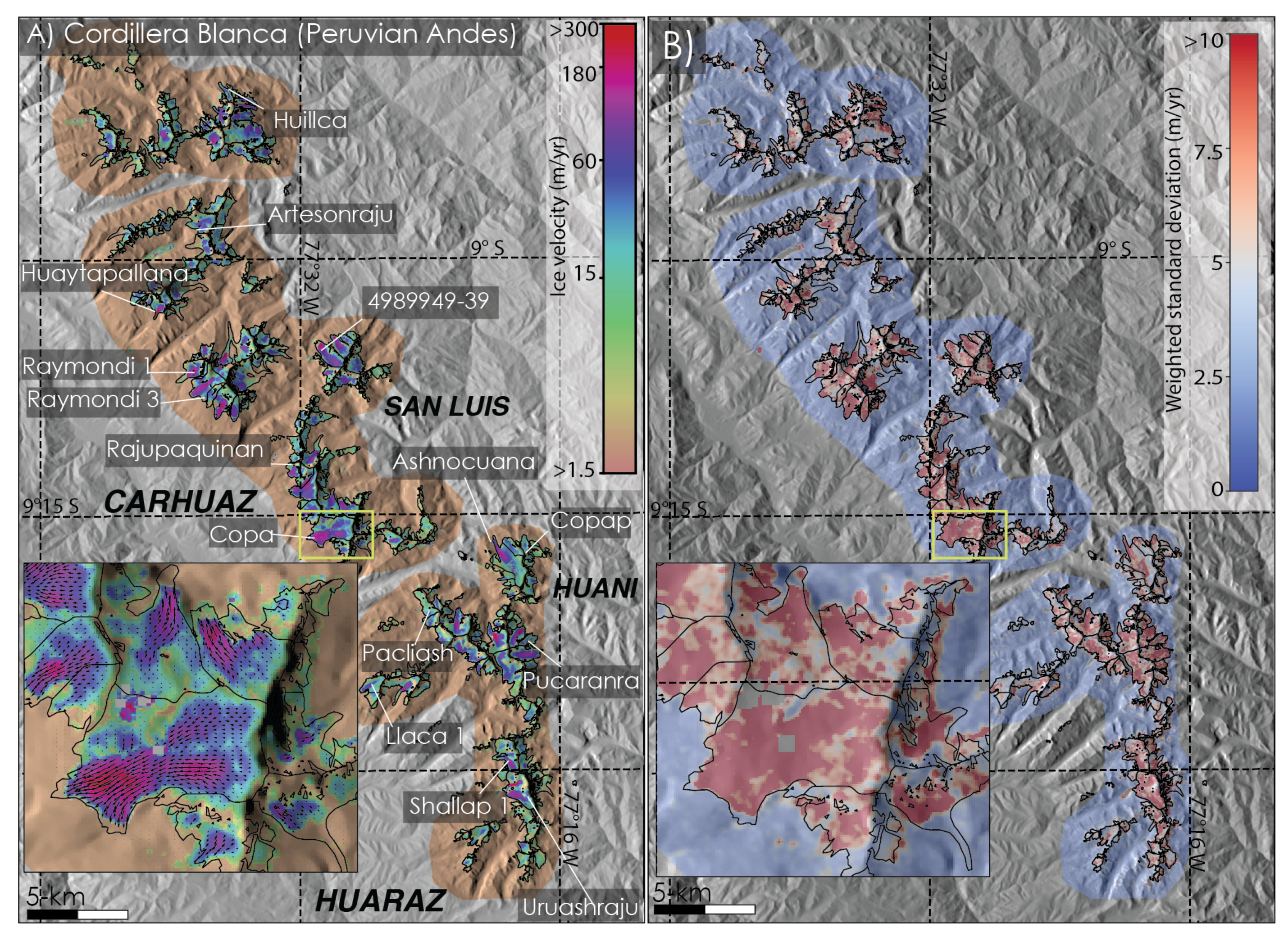
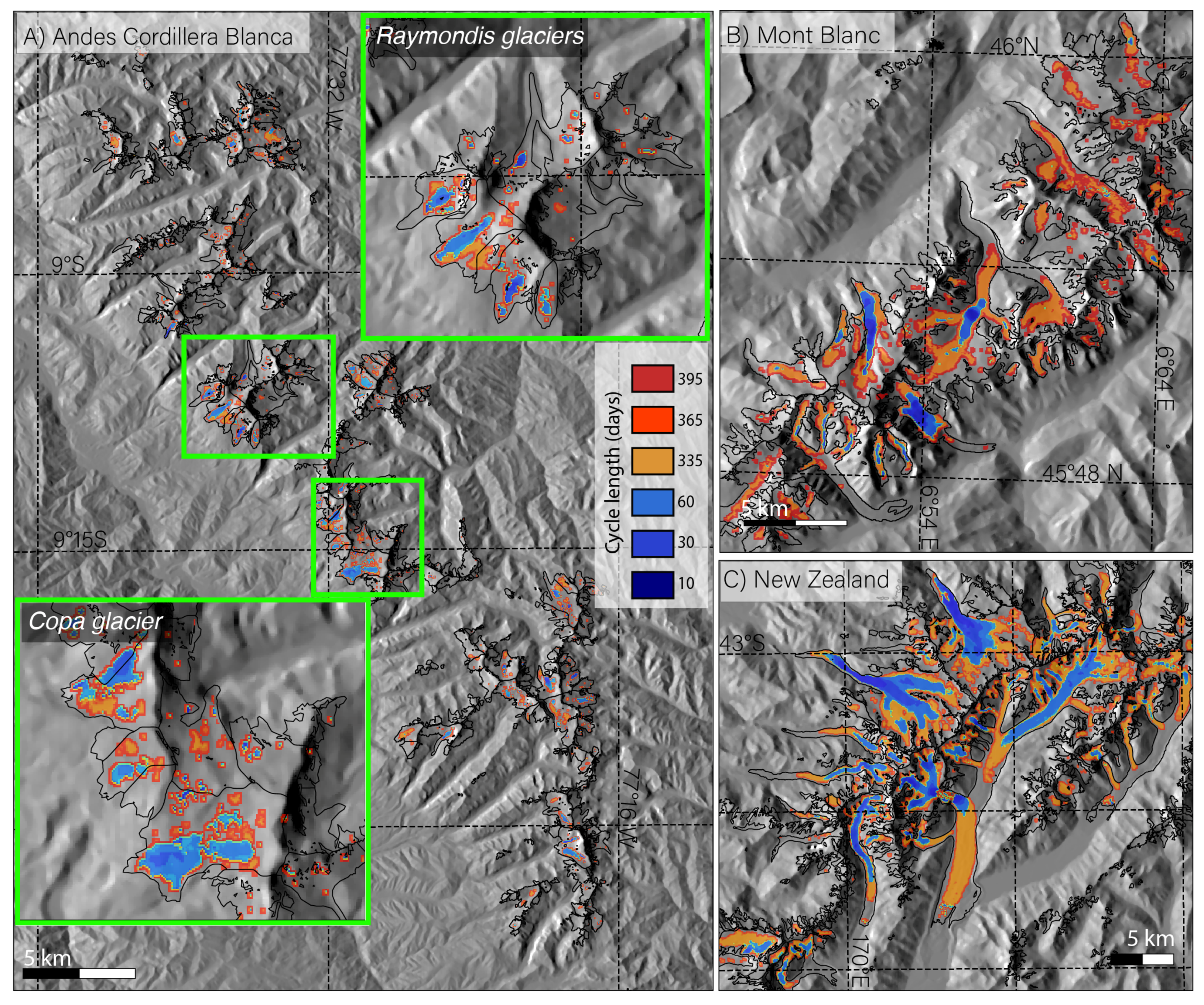
3.1.1. Peruvian Andes

Figure 1A presents the first complete high-resolution mapping of the surface speed of the glaciers of the Cordillera Blanca, located in the Peruvian Andes, from more than 5300 pairs of Sentinel-2 images. This region is characterized by glaciers of a typical length of 1 to 3 km, reduced ablation zones surrounded by steep mountain walls [30]. The variance or standard deviation in surface displacement (Figure 1B) varies from 1 to 3 m/year over ice-free areas and can reach more than 10 m/year over glaciers, which probably represents not only sensor noise but also significant changes in surface speed that can occur during the year due to seasonal changes and local climatic conditions. We note that a much smaller number of image pairs were processed on the eastern side of the mountain range, as shown in Figure S4A, with only 150 to 200 successful pairs compared to more than 500 on the western side of the cordillera. We attribute this difference to the higher probability of cloud cover from the Amazon basin to the east. As a result, the time average map value on the eastern side of the cordillera is less precise than in the western part.
The southern part of the Cordillera Blanca shows small glaciers and glacier surface velocity generally ranging from 30 to 150 m/year. The maximum glacier surface velocity derived from Sentinel-2 data is measured at the ice fall of an unnamed glacier west of Pucaranra with a speed of 305 m/year (Figure 1A). For the northern part of the Cordillera Blanca, in the vicinity of glaciers Huillca and Artesonraju, glacier surface velocity shows values typically ranging between 30–80 m/year, except for Huaytapallana, with a speed of 290 m/year in the ice fall. The fastest glaciers of the Cordillera are located in the central part with the Raymondi glaciers (12 km 2 ), Copa (11 km 2 ) and 4989949-39 (5 km 2 ), that all have glacier surface velocity above 100 m/year, homogeneously spread all along the ice tongue up the steep mountain peaks surrounding the accumulation region.

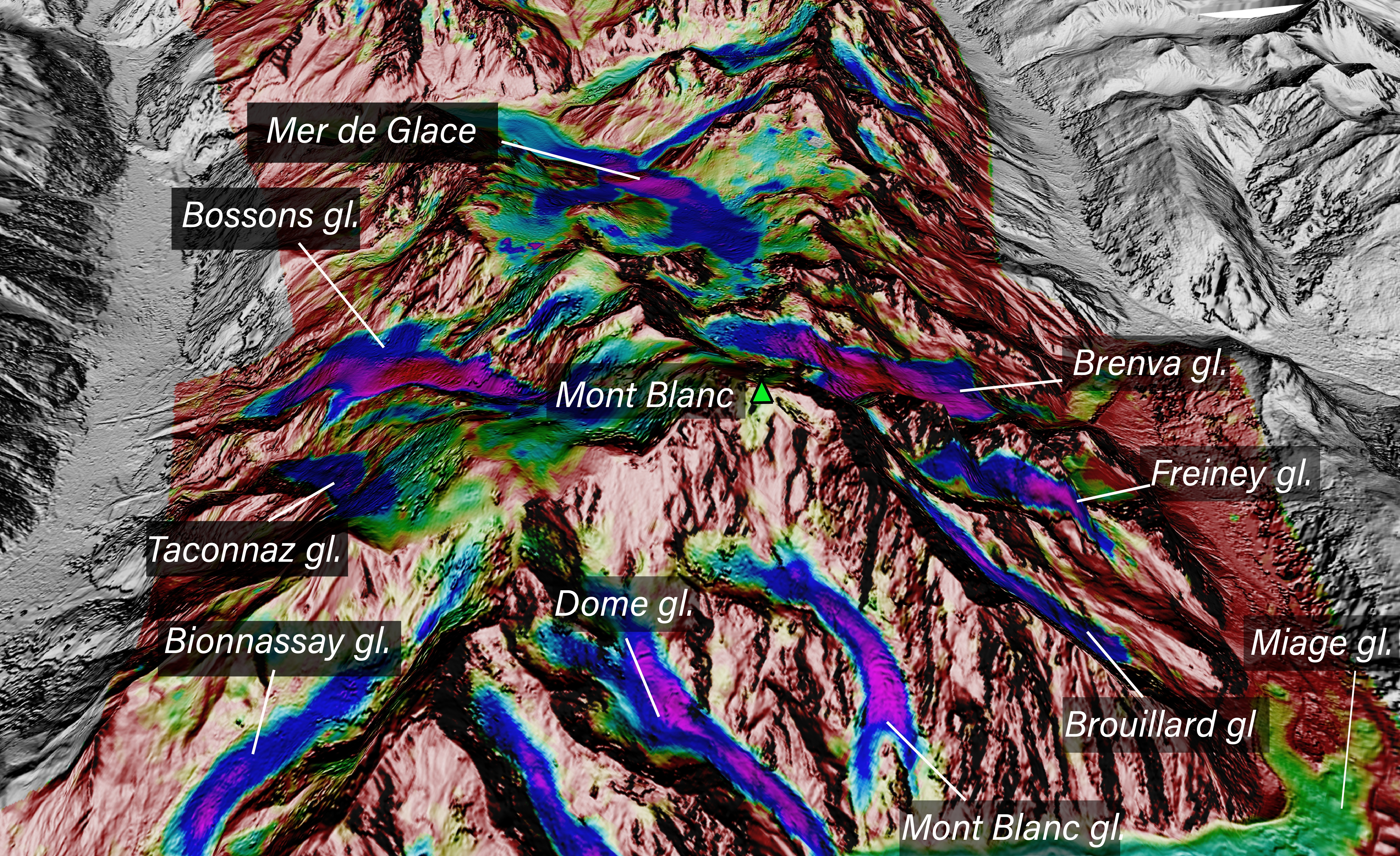
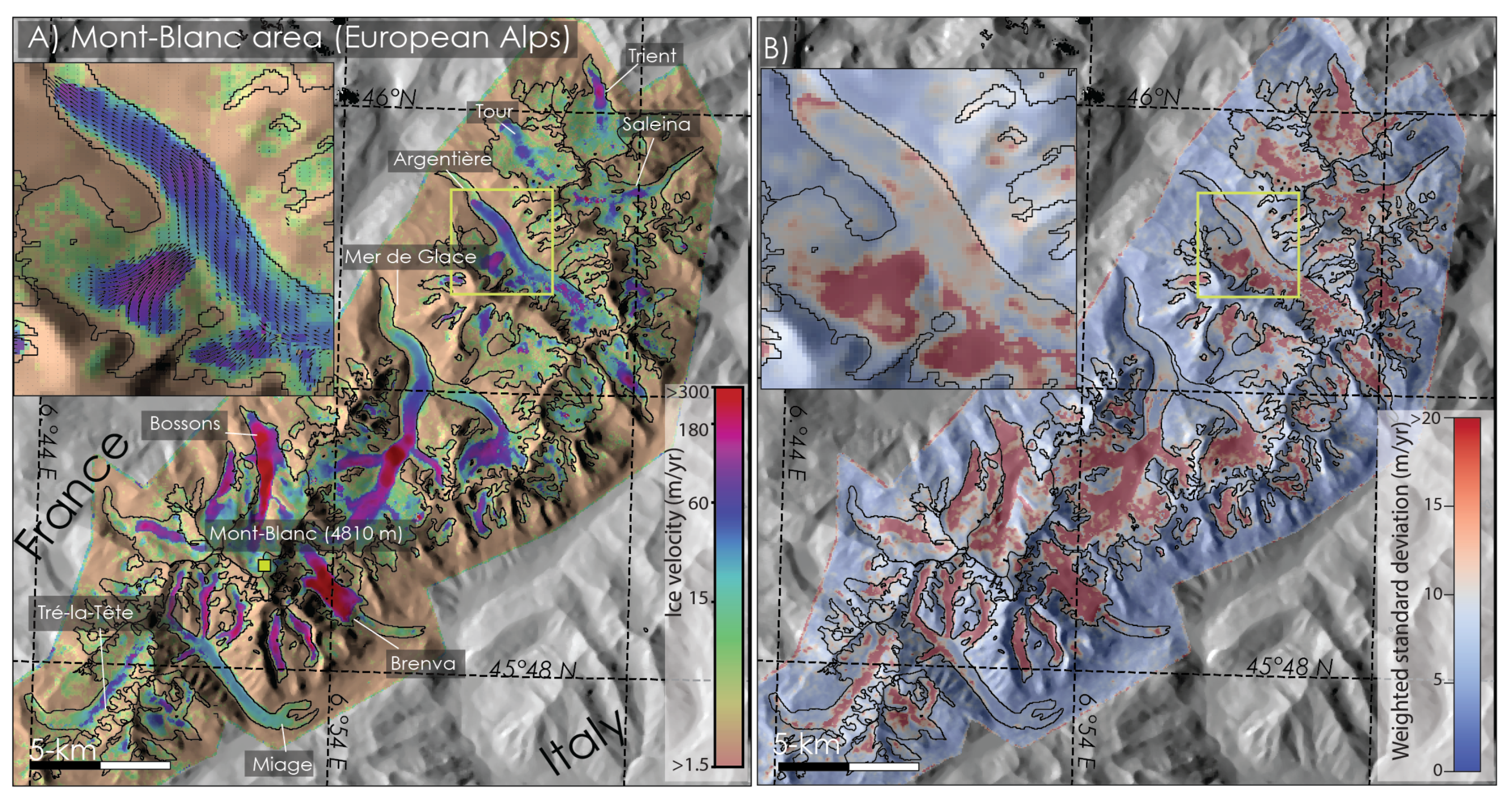
3.1.2. Mont-Blanc Area in the French Alps

The Mont-Blanc massif, located in the French Alps, includes some of the largest glaciers in the European Alps with the Mer de Glace (30 km 2 ) and Argentière (14 km 2 ) flowing into the Chamonix valley, the Miage glacier flowing towards Italy and the Tré-La-Tête glacier at the southern tip of the massif. However, the fastest surface velocities are observed for smaller glaciers with steep surface slopes, such as the Bossons glacier or the Brenva glacier on the Italian side with velocities above 350 m/year (Figure 2A). We found that the surface speed of the Mer de Glace is on average 70 m/year in the lower part of the glacier tongue while exceeding 500 m/year in the ice fall below the equilibrium altitude (ELA) (Figure 2A), in agreement with previous measurements made with SPOT-5 images [11]. The Argentière glacier also flows at about 70 m/year into the lower end of the glacier tongue (Figure 2A). We notice that the upper part of the glacier is almost constantly shaded with less surface features, resulting in fewer successful matching pairs and therefore higher uncertainty (Figure 2D). In general, it is noted that the areas with small standard deviations (1–2 m/year) are those with the gentlest slopes (i.e., Argentière, Mer de Glace, tongue of the Miage glaciers), where the largest number of successful matching pairs are obtained (>300) (Figure S4B).

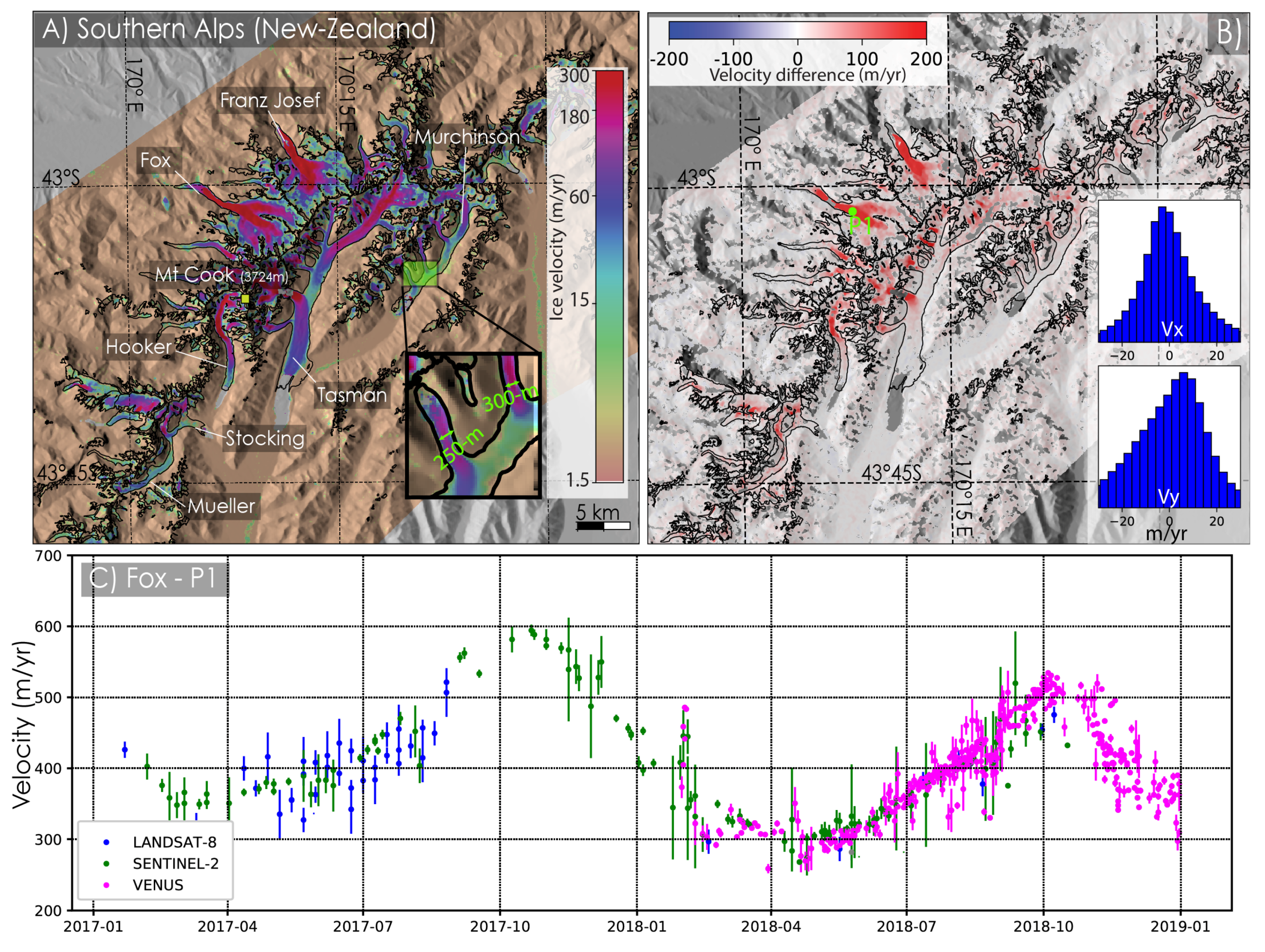
3.1.3. New-Zealand Southern Alps

The largest glacier-covered area in New-Zealand is located in the Aoraki/Mount Cook peak in the Southern Alps mountain range in the South Island. The largest glacier in this area is the Tasman Glacier (95 km 2 ) with a length of 26 km, and a 2-km width ice front that flows into the Tasman pro-glacial lake, south of Mt Cook. Glacier surface velocities of 250 m/year are observed in the ice fall close to the accumulation area while, the lowermost portion of Tasman is relatively slow with a speed of 60 m/year (Figure 3A). Two heavily crevassed glaciers with steep surface slopes are flowing on the northern flank of Mt Cook: Franz Josef and Fox glaciers with surface velocities reaching 500 m/year in some areas (Figure 3A). We also successfully mapped the tributaries flowing into Tasman, Hooker and Murchison glaciers with surface velocity ranging from 80–300 m/year.

3.2. Seasonal Variations in Glacier Surface Velocity

We found significant changes between summer and winter of glacier surface velocities (Figure 3B) along the main trunk of Fox, Franz Joseph, Hooker and Tasman glaciers. Differences between summer and winter speeds reach up to 150–200 m/year. We are confident that these values are significative as we find the median value in ice-free zones is −1 ± 16 and 1.6 ± 18 m/year for the x and y component, respectively (inset graphs in Figure 3B). Additionally, we plotted a 2-year time series in a fast flowing zone of Fox Glacier (noted P1 in Figure 3B,C), a glacier where seasonal field surface velocity have been measured in previous studies [25,31]. The strong seasonal signal is clearly highlighted in the time series: the maximum glacier surface velocity is recorded during the wettest period of the year [32] in late November 2017 with a velocity of 560 m/year and the minimum is measured in June 2018 with 280 m/year, resulting in a decrease in the surface velocity by 45%. Our 2-year record is consistent with previous studies [31] that used GPSs to measure a 26% (vs. 25% for this study) decrease between January–February and June–July. Note that the Ven μ s satellite also captured a short acceleration in ice velocity in February 2018, where the ice velocity quickly increased from 400 m/year to 480 m/year. Such changes in glacier flow might be explained by changes in subglacial hydrology between the spring/summer and fall/winter seasons that modify the basal slip [33,34]. Modifications in conditions at the base of the glacier are often due to changes in runoff that varies with the melt season but also with the amount of precipitation that can trigger important changes in the glacier flow velocity up to 44% [31,33].

3.3. Uncertainties Analysis

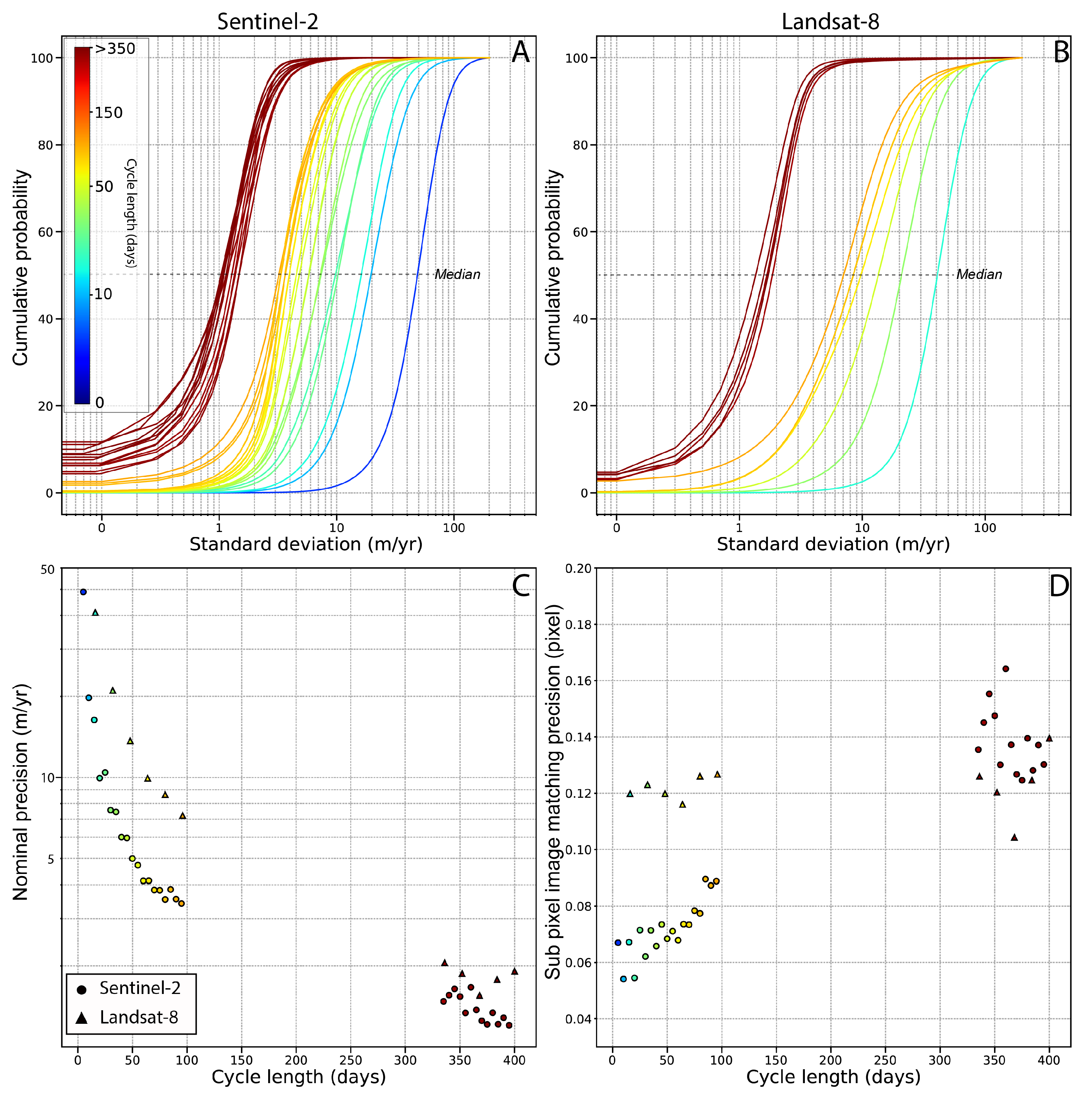
3.3.1. Sensor Precision

For each repeat cycle and each pixel of Landsat and Sentinel time-averaged maps, we calculate the filtered average surface velocities and its standard deviation as described previously in Section 2.4. The weights applied to the standard deviation and average calculations have no effect here as each mosaic is computed with the same repeat cycle and sensor. As output values are provided separately for x- and y-component, we combine them by taking the norm. The statistics presented in this section are calculated over the entire study regions (European Alps, Cordillera Blanca, New Zealand), hence over areas larger than the mosaics presented in Figure 1, Figure 2 and Figure 3 in Section 3.1 (see Figures S2 and S3). Figure 4A represents the cumulative distribution of the standard deviations (per pixel) of ice-free areas for different repeat cycle lengths. We assume that the 50th percentile of the standard deviation distributions (the median value of the distribution) represents the nominal precision that can be achieved for each cycle (Figure 4C). For comparison, we also calculated the mean of the distribution, which is about 1 m/year larger than the value of the median, hence do not impair our error analysis. Note that precision in glacierized areas is probably larger (less precise) than in ice-free zones because the surface texture is different and changes (e.g., snow precipitation, surface melt) can occur more rapidly, therefore causing more decorrelation. As glacier motion can changed rapidly over short time scale, the standard deviation over the glacier-covered areas does not necessarily represent the sensor precision but, more likely, natural fluctuations of the surface displacement. Nevertheless, we believe that our analysis on stable ground is valid to compare sensors precision and still provide insights on the capability of each sensor to map slow-moving mountain glaciers.
As expected, the precision on ice speed measurement increases with time separation between two acquisitions (at the expense of temporal resolution). Typically, precision for Sentinel-2 is about 52 m/year for a repeat cycle of five days and changes exponentially to 16.5, 7.8, 4.0, 3.5, 1.6 and 1.1 m/year for 10, 30, 60, 90, 335 and 390 days, respectively. For Landsat 8, we also found that the nominal precision is about two times larger than for Sentinel-2. Thus, displacement derived from Landsat repeat cycles of 16, 64, 96, 336 and 400 days can be mapped with a precision of about 41, 9.9, 7.2, 2 and 1.9 m/year, respectively. Hypothesizing that these values depends only on image correlation, we can calculate the sub-pixel image matching precision as m p = ( σ c y c l e / 365 . 25 ) × ( c / p s ) , where σ c y c l e is the standard deviation of a given cycle, c is the cycle length and p s the pixel size. We found that our correlation algorithm has a sub-pixel precision of about 0.1 pixel, which matches our earlier assumption for the calculation of the weights (Figure 4D) and is similar to [29,35]. For Sentinel-2, correlation tends to perform better for short repeat cycles (about 0.06 to 0.09 pixel matching precision) than for long repeat cycles (about 0.13–0.16 pixel matching precision), which is expected as change in surface texture will be larger for longer cycles. This relationship between the precision and the cycle length is however not as clear for Landsat 7/8 (Figure 4D).
In the case of the Mont Blanc massif, we also analyzed the weighted standard deviation obtained in the ablation and accumulation zones computed for the time-averaged maps of the glacier surface velocity, which contain all repeat cycles. Ablation and accumulation zones may have different surface textures impacting the correlation algorithm. We used the altitude of the equilibrium line (ELA) from [36] located around 3000 ± 100 m.s.l. in the French Alps to distinguish the ablation and accumulation zones. For the Bossons and Brenva glaciers, where we have a relatively homogeneous number of matching pairs, similar precision is estimated for both zones (15–20 m/year). On other glaciers, we observe differences in precision that do not seem to be completely related to the accumulation or ablation zones. For example, in the lower parts of the Mer de Glace and Miage glaciers that have a gentle slope and where the surface speed is less than 50 m/year, the weighted standard deviation is only 2–4 m/year, thus close to the nominal precision calculated on a stable ice-free ground. Above the altitude of 2400 m, however, the terrain becomes steeper, shows greater spatial variability in ice flow and has fewer surface features to follow due to the presence of snow. This results in larger weighted standard deviations, at the order of 15–20 m/year. Another example is the Argentière glacier, where the weighted standard deviation starts to increases considerably dowstream of the ELA (2700 m), where the glacier surface is in the shade of the Aiguille Verte and Droites peaks. In summary, several factors can affect the precision of surface speed estimates: seasonal flow variability, shaded areas, steep slopes, difficult weather conditions (resulting in significant cloud cover) and, most importantly, the absence of surface features due to permanent snow cover. On average for the French Alps, we found a weighted standard deviation of 12.4 m/year in the accumulation zone compared to 12.8 m/year in the ablation zone (Figure 2C), highlighting, for the reasons stated above, the difficulty of estimating the nominal sensor precision for displacement mapping using areas covered by glaciers.

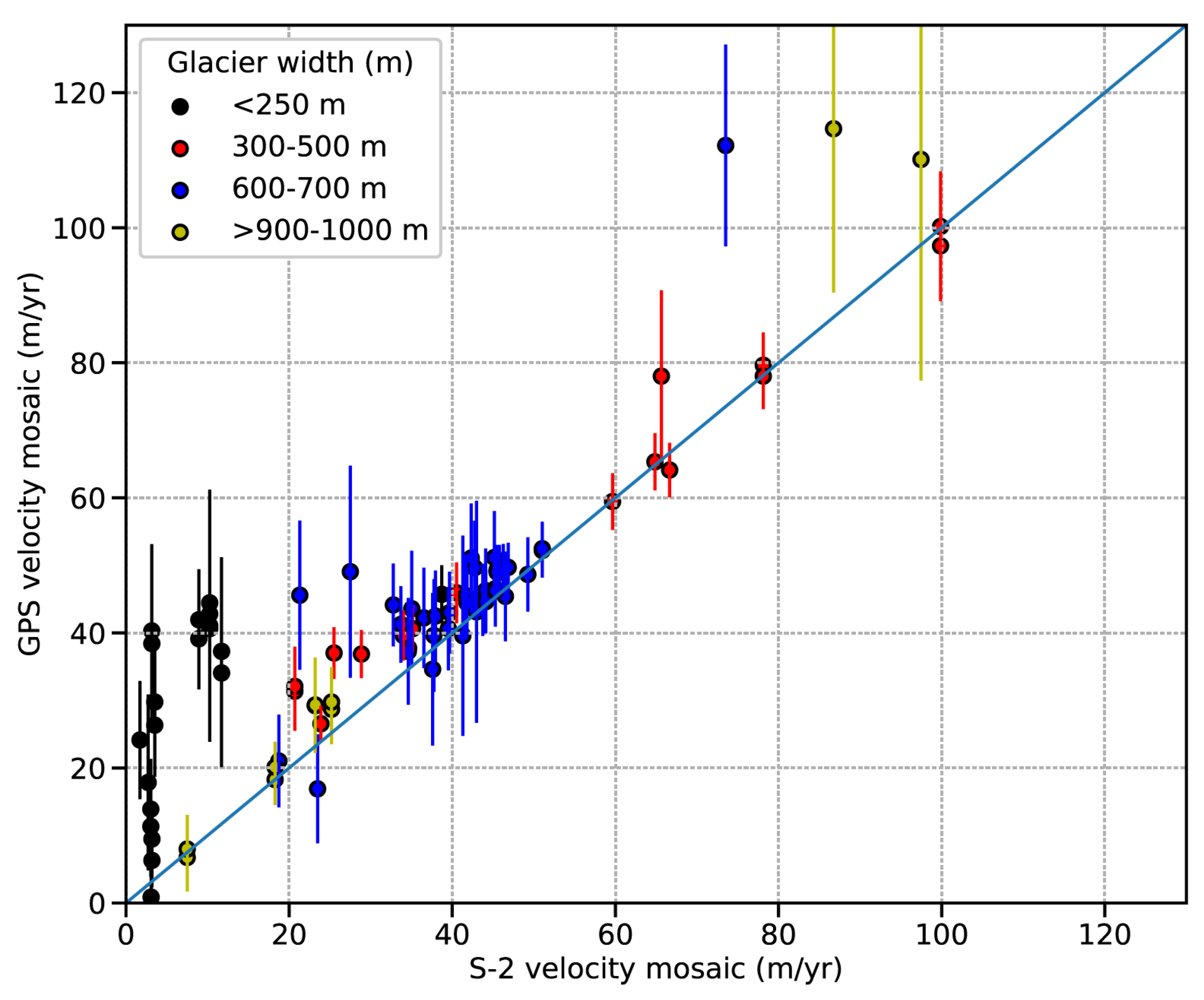
3.3.2. Comparison between GPS Measurements and Sentinel-2

Comparison of annual glacier surface velocities obtained from in-situ differential GPS measurements and from Sentinel-2 2017–2018 time-averaged map shows good overall agreement as illustrated in Figure 5. The color of the GPS points in the figure characterizes the width of the glacier. We note that the largest discrepancies are observed for glaciers with width of less than 250 m, which are not well captured by our processing chain. We also note important differences for three GPS points located in the accumulation area of the Mer de Glace glacier, where only a small number of successful pairs were obtained, hence with a large weighted standard deviation due to the poor statistic (see Section 3.3.1 and Section 3.1). Similar pattern can also be observed for Argentière Glacier (Figure S5). Our mapping agrees within 5% in the ablation zone (close to point A’, km 3.5 to km 4.25 in Figure S5) where a robust statistic of more than 200 estimates is found and weighted standard deviation is about 10 m/year. Higher upstream (close to point A, km 0.25 to km 1 in Figure S5), image matching is more complex because of the limited number of surface features and the persisting shadows cast by steep surrounding mountains. The poor statistic in this area translates into noisier pattern of ice velocity and larger difference between GPS and Sentinel-2 measurements of about 10 m/year.
Overall, the mean difference, calculated as the weighted average of the differences between the GPS and Sentinel-2 points, is 6 m/year. The weights are defined as the inverse of the local precision estimated with Sentinel-2 (see Section 3.3.1), GPS measurements are assumed to provide the actual displacement and therefore error-free. If we do not consider glaciers less than 250 m wide, the difference is only 3.7 m/year because, as mentioned above, these glaciers are not well captured by our processing chain. Although the number of comparisons with GPS measurements is statistically low, this suggests that the accuracy of the Sentinel-2 time-averaged map would be less than 10 m/year. The remaining discrepancies could also be due to the difference in time periods between the GPS measurements acquired between 2015–2017 and our map, which is representative of the years 2017 and 2018. Another reason for the differences between in-situ and remote measurements would obviously be the resolution of our map (50 m) which will necessarily spatially “smooth” the motion compared to local GPS measurements.

3.3.3. Comparison between Sentinel-2 and Ven μ s in the Southern Alps of New Zealand

For glaciers in the Mount Cook area in the Southern Alps of New Zealand, we can compare the performances of Sentinel-2 (Figure 3A) with the 5-m spatial resolution Ven μ s satellite (Figure 6A). To do this, we formed a time-averaged ice velocity map from the Ven μ s images. The resulting map is shown in Figure 6A. Note that we observe a clear step in background velocity from Ven μ s due to the change of the acquisition footprint that was enlarged after November 2018 (before, the footprint was more focused on Tasman Glacier), hence fewer data are available in these newly covered zones. Similarly to Sentinel-2 (Figure 4C), we estimate the Ven μ s nominal precision for each cycle from the distributions of the weighted standard deviation in ice-free areas (Figure 6B). The evolution of the precision with the repetition cycle obtained for Ven μ s is similar to that of Sentinel-2 (Figure 6B), while we expected that the accuracy of Ven μ s would be better due to the increased spatial resolution (5 m versus 10 m for Sentinel-2). We attribute the lower performance of Ven μ s to the quality of the image ortho-rectification. This is however largely compensated by the number of acquisitions (every 2 days) that can be stacked and helps to capture finer temporal details (Figure 6A).

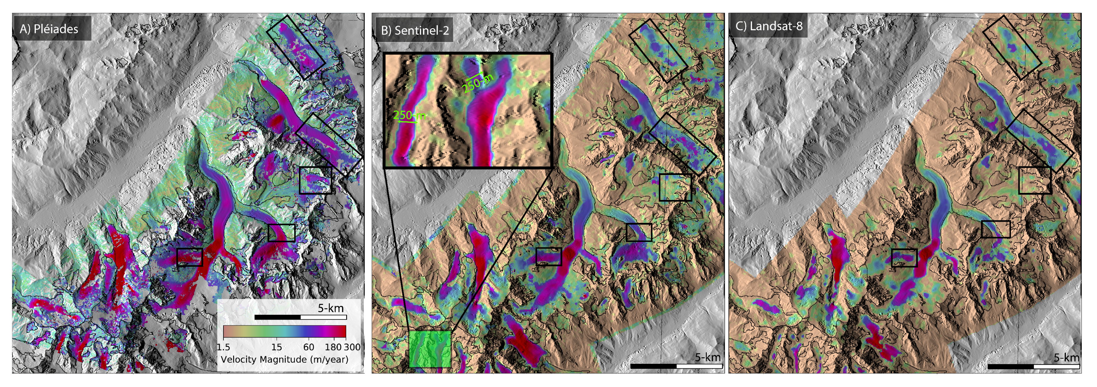
3.3.4. Comparison between Sentinel-2, Landsat, Planet Labs and Pléiades in the French Alps

On the Mont Blanc massif, we can compare the Landsat 8 and Sentinel-2 data with the 50 cm resolution Pléiades sensor obtained as part of the CNES/Kalideos-Alpes project and the measurements made from Planet images.
We use a surface flow velocity map made from a pair of Pléiades images that were acquired 30 days apart during the summer of 2018 and compare it to time-averaged maps derived from Sentinel-2 and Landsat 8 to assess the level of detail obtained by the latter (Figure 7). We find that the overall spatial distribution of glacier surface speed is preserved on the Landsat 8 and Sentinel-2 maps with respect to Pléiades. Obviously, Pléiades offers a sharpness in the displacement map that cannot be obtained with sensors that acquire images at a spatial resolution 20 to 30 times lower. This is particularly true along glacial margins and for narrow glaciers such as the upper reaches of the Mer de Glace, and for tributaries of the Miage Glacier (inset Figure 7B). There are some differences in the upper part of the Argentière glacier where few elements can be followed and/or frequent shading is present, and where Pléiades offers better performance (Figure 7). We estimate that the precision on displacement over ice-free areas is 4.3 m/year for Pléiades, while the Sentinel-2 and Landsat 8 maps reach this level of precision for cycles longer than 60 and 160 days, respectively (based on Figure 4C). Note that, to obtain these details, a considerable number of image pairs must be used for Sentinel and Landsat, whereas with Pléiades we used only one pair. This highlights the advantages and need for very high resolution sensors such as Pléiades to map with high accuracy the smallest mountain glaciers that are not currently captured by conventional sensors.
We can also use the data from Planet Labs which provides orthorectified intermediate resolution images of 3 m and compare the ice speed maps produced by this sensor with those of Sentinel-2 (10 m) and Pléiades (50 cm). We obtained 15 pairs of images between April 2018 and September 2018 with different observation geometries (for example, not in the same orbit) from Planet Labs. Due to the limited number of images that are freely accessible, we are not able to perform the same statistical analysis on sensor precision as for Ven μ s, Sentinel-2 and Landsat by calculating the standard deviation for each pixel between the different measurements. However, we have estimated the standard deviation of displacement on ice-free areas for each pair of images (Figure S3) and find a value of 50 m/year for a 7-day repetition cycle, decreasing exponentially to 15–20 m/year for 40 to 50-day cycles (Figure S6). These values are higher than those expected for 3 m spatial resolution imagery and are attributed to ortho-rectification issues that are exacerbated by the fact that we were unable to use exactly the same orbital paths between image pairs. We believe that additional geometric corrections are therefore necessary to fully utilize the potential of Planet Labs images.

3.3.5. Comparison with Existing Regional Ice Velocity Datasets

In Figure 8, we compare our Sentinel-2 2017–2018 time-averaged speed map with a map generated from Landsat GoLIVE data available over the Mont Blanc massif [15,37]. We oversample each GoLIVE ice velocity at a resolution of 50 m and follow the same post-processing methodology described in the Section 2.4 (Figure 8). We also compare the results with a previous Landsat 8 map published by [38] that uses a processing chain similar to ours in terms of the parameters used for correlation [24]. Our map like the one in [38] seems to better capture the main glaciers of the Mont Blanc massif such as the Mer de Glace or Leschaux glaciers, with shear margin transitions that are better defined than GoLIVE. It also appears that many small glaciers are not visible in the GoLIVE map, as for example on the Italian side of the massif with the Rochefort and Planpincieux glaciers.

3.3.6. Minimum Time Interval for Time Series Analysis with Sentinel-2

Finally, we have tried to establish the required minimum repetition cycle for Sentinel-2 that would allow to detect a 10% change in glacier surface velocity, which generally corresponds to the expected variation in glacier velocity with the seasons. We assume that this requirement would be met when the 2- σ precision of the velocity maps (Figure 4C) is smaller than one-tenth of the magnitude of the ice flow, which would therefore provide a sufficient signal-to-noise ratio to capture the variation. Illustrated in Figure 9, this analysis shows a consistent pattern between the length of the cycle to be used and the magnitude of the glacier’s surface velocity: long cycle lengths are required in slow areas of the glaciers while short cycles can be used in the fastest. For example, a minimum ten-day repetition cycle would be required for glacier surface speed time series at speeds greater than 400/year (e.g., Figure 9C, Fox Glacier), a repetition cycle greater than 30 days would be required to capture glacier flow at a rate of 200–400 m/year (typically the Bossons and Mer de Glace glaciers in Figure 9B) and lower glaciers at speeds of 100–200 m/year should be monitored with 60-day or longer cycles. In summary, this highlights the current limitations of Sentinel-2 (and therefore Landsat 8) of capturing seasonal variations for glaciers flowing at a rate slower than 100 m/year, i.e., 10 m/year speed change, which is the case for the large proportion of the glaciers of the study regions: the European Alps, the Cordillera Blanca in the Peruvian Andes and the southern Alps of New Zealand).

4. Discussion

We implemented a workflow to process datasets from several optical sensors, we generated time-averaged maps of glacier speed from Sentinel-2 data and compared the results with those of other sensors: Landsat 8 with a slightly lower sensor resolution and Ven μ s, Planet Labs and Pléiades with a higher spatial resolution. We tried to evaluate the performance of Sentinel-2 against other optical sensors to map the surface speed of mountain glaciers in three regions of the world with glaciers having distinct morpho-topographical characteristics.
Our statistical analysis shows that the glacier surface velocity precision is exponentially improved with increasing cycle length. We note that calculating velocity fields with pairs that have repeat cycles greater than 335 days provides highly precise velocity maps but does not significantly improve the precision (Figure 4C). For example, we found that Sentinel-2 provides glacier surface velocity with a precision 1.5 to 2 times greater than Landsat, which can be attributed to the better resolution of Sentinel-2 (100 m 2 per pixel versus 225 m 2 ). We show that, with Sentinel-2 or Ven μ s (Figure 9), time series of flow velocities can be produced at a frequency of 10 days with a signal-to-noise ratio sufficient to capture variations of about 40 m/year, typically for glaciers with speeds greater than 400 m/year. However, speed fluctuations in the order of 10–20 m/year and 20–40 m/year can only be monitored with a reasonable signal-to-noise ratio at a monthly to quarterly time scale (Figure 8), and capturing fluctuations below 10 m/year remain challenging, if not impractical because only a repeated cycle longer than 100 days would be effective (Figure 8). At present, the precision achieved for the nominal repeat cycles (5 days for Sentinel-2, 2 days for Ven μ s and 16 days for Landsat) is not enough to capture most of the glacier speed changes, typically for glaciers flowing below 200 m/year (Figure 1 and Figure 2, Figure 4C and Figure 6C). Therefore, these sensors with 5 to 15-m spatial resolution might be limited for catching rapid speed fluctuations smaller than 50 m/year. We note that these data are however perfectly suited for faster flowing glaciers with surface velocity >500 m/year [14,28,39].
As expected, the 50 cm spatial resolution Pléiades images completely outperform the precision achieved by other conventional sensors (Sentinel, Landsat) that have a resolution at least 20 times coarser. The glacier surface velocity fields obtained from Pléiades are ideal to document detailed surface velocity patterns (shear margins, small glaciers, tributaries) and to monitor short term variations in the dynamics of mountain glaciers (Figure 8). However, the production of glacier surface velocity maps with Pléiades requires longer processing time, with additional stereo or tri-stereo processing steps, and larger search windows during the cross correlation. With a potential repeat cycle of 1-day, this high-resolution sensor would be the perfect tool for mountain glaciers, but is currently limited because of the non-systematic, non-global acquisitions and commercial access [40].
Although one would have expected a higher precision due to the improved spatial resolution of Ven μ s compared to Sentinel-2, the similar precision obtained is probably due to the larger errors in the orthorectification of Ven μ s data. These orthorectification errors are mainly the result of slight changes in the angle of view due to frequent changes in the satellite’s orbit during tests carried out on the satellite electric engine (Gérard Dedieu, pers. comm., 2018). Therefore, a high-resolution and highly accurate digital elevation model would be required to obtain the best possible orthorectification of Ven μ s images, which should significantly improve glacier surface velocity maps. Due to this limitation, it is not yet possible to draw conclusions on the benefits of the higher spatial resolution provided by the Ven μ s data for mapping glacier surface velocity. On the other hand, since the issue of orthorectification seems random (not systematic), the high temporal resolution of Ven μ s (2 days) acquisitions can however be used to generate precise time-averaged map. In addition, Ven μ s will undoubtedly help to improve the time series of glacier speed, as shown in Figure 3C, where Ven μ s captures a short-term acceleration of the Fox Glacier with more details than Sentinel-2. In the case of Planet Labs’ satellite constellation, our analysis shows similar problems to those of Ven μ s for the quality of orthorectification of images. However, with additional corrections for uncompensated stereo effects, the Planet Labs data have interesting potential for mapping glacier surface velocity.
These results highlight the importance of having frequent acquisitions with very high resolution sensors and an accurate ortho-rectification in order to capture the changes in surface velocity of small mountain glaciers. It also shows that Sentinel-2 and Landsat 8 are able to capture with enough details and precision the main glaciers of the world glacier-covered massifs for future studies. Thus, we showed from the comparison with very high resolution sensors and GPS measurements that ‘conventional’ sensors (Sentinel and Landsat) capture surface flow velocity for most glaciers larger than 250 m (Figure 3 and Figure 5, Figure 6 and Figure 7). Currently, Pléiades, Planet Labs or Ven μ s can locally improve the large scale acquisitions from Sentinel-2 and Landsat 8 and therefore supplement the record of glacier dynamics at even finer spatial and temporal scales.
When sufficient amount of data are available and stacked, we found a good agreement between GPS and satellite derived glacier surface velocity for glaciers that are at least 250 m wide (Figure 5), suggesting that the accuracy of the Sentinel-2 time-averaged map would be less than 10 m/year. Glacierized areas with persistent shade, snow cover and/or limited number of surface features still remain challenging for Landsat 8 and Sentinel-2 where precision and accuracy are much lower. The use of an orientation correlation algorithm as described in [26], could potentially improve ice velocity mapping in such regions with strong changes in image intensity. Additional post-processing filtering, for example based on the flow direction of the velocity vector, could be envisioned in future implementations and would certainly improve the final velocity product or time series analysis [8,41].
We have shown that, by combining all possible repetition cycles, Sentinel-2 or Landsat 8 can be used to produce time-averaged maps at a spatial resolution of 50-m with enough detail to capture most individual mountain glaciers (Figure 1, Figure 2 and Figure 3). Although the native resolution of Sentinel-2 and Landsat 8 remains a limitation for capturing smaller glaciers (<250 m wide), we observe a gain over existing Landsat 8-based databases for mapping mountain glaciers. We attribute this difference to the higher spatial density of the offset maps generated here and the higher resolution of Sentinel-2 compared to Landsat 8. We note that with our approach, each correlation of offset maps is not independent of these direct neighbours. However, it would seem that this approach provides more convincing results than interpolating correlation maps generated on a coarser grid. Our data processing and use of Sentinel-2 data therefore provides improved mapping of mountain glaciers compared to existing global ice speed products such as the GoLIVE project [15,37]. These improved maps of glacier surface velocity will certainly be useful for glacier flow modelling, mass conservation techniques or any other applications using glacier surface velocity as input data. For example, it has been shown that knowledge of glacier flow is an effective constraint to calculate the distribution of glacier thickness while preserving the true shape of glacial valleys [7,8,42].

5. Conclusions

In this manuscript, we describe a new multi-sensor processing chain for processing a large amount of optical satellite data used to map the surface flow velocity of mountain glaciers on a regional scale. We present the first complete maps of glacier surface speed at a resolution of 50 m for the Peruvian Cordillera Blanca (tropical Andes), the European Alps and the Southern Alps of New Zealand. We performed a statistical analysis to establish the precision of Sentinel-2 and Landsat 8 for different repeat cycles. We conclude that the precision of glacier surface velocity mapping is 1.5 to 2 times better with Sentinel-2 than with Landsat 8 for similar repetition cycles, as expected by the better resolution of Sentinel-2. Our estimation of Sentinel-2 precision indicates that only glaciers with ice velocity fluctuations greater than 10 m/year can be monitored on a seasonal basis. We also estimate that, with Sentinel-2 or Landsat 8, the best temporal resolution that can be achieved is about 10 days for speed variations of about 40 m/year. When all the processed pairs are stacked together, we demonstrate the ability of our processing chain to derive the time-averaged ice flow with an accuracy between a few meters per year and about ten meters per year. However, we note that Sentinel-2 and Landsat 8 cannot capture the smallest glaciers (<250 m wide) and that snow-covered accumulation areas remain challenging. By comparing Sentinel-2 mappings with those obtained by Pléiades and Ven μ s, we have shown that the latter can still provide a benefit for mapping time-varying glacier surface flow. The products presented in this study will be available on the THEIA platform.

Supplementary Materials

The following are available online at: https://0-www-mdpi-com.brum.beds.ac.uk/2072-4292/11/21/2498/s1. Figure S1: Example of ice velocity map and the related percentage of filtered values, remaining values after filtering for 0.5- σ , 1- σ , 2- σ and 3- σ parameters; Figure S2: Surface velocity of glaciers in the European alps. Background image is from Google Earth. Surveyed areas are in yellow. Insets show a zoom on selected areas where the glacier surface velocity is represented on a logarithmic scale going from brown (slow) to red (fast) and overlaid on a shaded relief version of the SRTM DEM; Figure S3: Surface velocity of glaciers in New Zealand. Background image is from Google Earth. Surveyed areas are in blue. Insets show a zoom on selected areas where the glacier surface velocity is represented on a logarithmic scale going from brown (slow) to red (fast) and overlaid on a shaded relief version of the SRTM DEM; Figure S4: Number of pairs processed at each pixel location, color coded from dark blue (low number of pairs) to dark red (high number of pairs) for Cordillera Blanca (A) and the Mont-Blanc region in the Europan Alps (B); Figure S5: Comparison between satellite-derived and differential GPS glacier surface velocities (identified as yellow dots) between 2016 and 2018 along the central flowline of Argentière Glacier in the Mont-Blanc area (European Alps). Displayed error bars are the weighted standard deviation (1-sigma). Background is the glacier surface velocity mosaic on a logarithmic scale from 1.5 (brown) to 300 m/year (red) overlaid on a CNES’s Pléiades ortho-image from 2017; Figure S6: Standard deviation on stable ground of the Planet labs glacier surface velocity mosaics as a function of the repeat cycle length.

Author Contributions

R.M., J.M. and A.R. designed the study. R.M., J.M., S.J. and M.C. designed the processing chain. R.M., J.M., D.C. and A.D. processed the data. R.M. performed the analysis. R.M., A.R. and J.M. wrote the article. All co-authors helped discussing and reviewing the article.

Funding

This research was funded by a CNES Post-doctoral fellowship, the CNES MaISON and Kalideos Alpes projects.

Acknowledgments

We would like to thank C. Vincent and the Service National d’Observation GLACIOCLIM (https://glacioclim.osug.fr/) for the availability of in-situ data on Argentière Glacier, G. Dedieu (Ven μ s), J.P. Dedieu (Pointing), NASA, ESA and CNES for the data availability. We thank the Planet Labs company for providing free images through their Ambassador program. This work was made possible thanks to the contribution of Labex OSUG@2020 (Investissements d’avenir - ANR10 LABX56). Thanks to E. Berthier and F. Brun for providing support with the Ames Stereo Pipeline. The computing/storage resources used for this work were provided by GRICAD (Grenoble Alpes Recherche - Infrastructure de Calcul Intensif et de Données).

Conflicts of Interest

The authors declare no conflict of interest.

References

  1. Church, J.A.; White, N.J.; Konikow, L.F.; Domingues, C.M.; Cogley, J.G.; Rignot, E.; Gregory, J.M.; van den Broeke, M.R.; Monaghan, A.J.; Velicogna, I.; et al. Revisiting the Earth’s sea-level and energy budgets from 1961 to 2008. Geophys. Res. Lett. 2011, 38, L18601. [Google Scholar] [CrossRef]
  2. Vaughan, D.G.; Comiso, J.C.; Allison, I.; Carrasco, J.; Kaser, G.; Kwok, R.; Mote, P.; Murray, T.; Paul, F.; Ren, J.; et al. Contribution of Working Group I to the Fifth Assessment Report of the Intergovernmental Panel on Climate Change; Cambridge University Press: New York, NY, USA, 2013. [Google Scholar]
  3. Riaz, S.; Ali, A.; Baig, M.N. Increasing risk of glacial lake outburst floods as a consequence of climate change in the Himalayan region. J. Disaster Risk Stud. 2014, 6. [Google Scholar] [CrossRef]
  4. Cuffey, K.M.; Paterson, W.S.B. The Physics of Glaciers; Elsevier: Burlington, NJ, USA, 2010. [Google Scholar]
  5. GlaThiDa Consortium. Glacier Thickness Database 3.0.1; World Glacier Monitoring Service: Zurich, Switzerland, 2019. [Google Scholar]
  6. RGI Consortium. Randolph Glacier Inventory(RGI)—A Dataset of Global Glacier Outlines: Version 6.0.; Technical Report; Global Land Ice Measurements from Space: Boulder, CO, USA, 2017. [Google Scholar]
  7. Farinotti, D.; Brinkerhoff, D.J.; Clarke, G.K.C.; Fürst, J.J.; Frey, H.; Gantayat, P.; Gillet-Chaulet, F.; Girard, C.; Huss, M.; Leclercq, P.W.; et al. How accurate are estimates of glacier ice thickness? Results from ITMIX, the Ice Thickness Models Intercomparison eXperiment. Cryosphere 2017, 11, 949–970. [Google Scholar] [CrossRef] [Green Version]
  8. Rabatel, A.; Sanchez, O.; Vincent, C.; Six, D. Estimation of glacier thickness from surface mass balance and ice flow velocities: A case study on Argentière Glacier, France. Front. Earth Sci. 2018, 6, 112. [Google Scholar] [CrossRef]
  9. Vuille, V.; Carey, M.; Huggel, C.; Buytaert, W.; Rabatel, A.; Jacobsen, D.; Soruco, A.; Villacis, M.; Yarleque, C.; Elison, O.T.; et al. Rapid decline of snow and ice in the tropical Andes—Impacts, uncertainties and challenges ahead. Earth Sci. Rev. 2018, 176, 195–213. [Google Scholar] [CrossRef]
  10. Beniston, M.; Farinotti, D.; Stoffel, M.; Andreassen, L.M.; Coppola, E.; Eckert, N.; Fantini, A.; Giacona, F.; Hauck, C.; Huss, M.; et al. The European mountain cryosphere: A review of its current state, trends, and future challenges. Cryosphere 2018, 12, 759–794. [Google Scholar] [CrossRef]
  11. Berthier, E.; Vincent, C. Relative contribution of surface mass balance and ice flux changes to the accelerated thinning of the Mer de Glace (Alps) over 1979–2008. J. Glaciol. 2012, 58, 501–512. [Google Scholar] [CrossRef]
  12. Wigmore, O.; Mark, B. Monitoring tropical debris-covered glacier dynamics from high-resolution unmanned aerial vehicle photogrammetry, Cordillera Blanca, Peru. Cryosphere 2017, 11, 2463–2480. [Google Scholar] [CrossRef] [Green Version]
  13. Millan, R.; Mouginot, J.; Rignot, E. Mass budget of the glaciers and ice caps of the Queen Elizabeth Islands, Canada, from 1991 to 2015. Environ. Res. Lett. 2017, 12. [Google Scholar] [CrossRef]
  14. Mouginot, J.; Rignot, E. Ice motion of the Patagonian Icefields of South America: 1984–2014. Geophys. Res. Lett. 2015, 42, 1441–1449. [Google Scholar] [CrossRef]
  15. Fahnestock, M.; Scambos, T.; Moon, T.; Gardner, A.; Haran, T.; Klinger, M. Rapid large-area mapping of ice flow using Landsat 8. Remote Sens. Environ. 2015, 185, 84–94. [Google Scholar] [CrossRef]
  16. Dehecq, A.; Gourmelen, N.; Gardner, A.S.; Brun, F.; Goldberg, D.; Nienow, P.W.; Berthier, E.; Vincent, C.; Wagnon, P.; Trouvé, E. Twenty-first century glacier slowdown driven by mass loss in High Mountain Asia. Nat. Geosc. 2019, 12, 22–27. [Google Scholar] [CrossRef]
  17. Beniston, M. Mountain weather and climate: A general overview and a focus on climatic change in the Alps. Hydrobiologia 2006, 562. [Google Scholar] [CrossRef]
  18. Stocker-Waldhuber, W.; Fischer, A.; Helfricht, K.; Kuhn, M. Long-term records of glacier surface velocities in the Oetztal Alps (Austria). Earth Syst. Sci. Data 2019, 11, 705–715. [Google Scholar] [CrossRef]
  19. Pfeffer, W.T.; Arendt, A.A.; Bliss, A.; Bolch, T.; Cogley, J.G.; Gardner, A.S.; Hagen, J.O.; Hock, R.; Kaser, G.; Kienholz, C.; et al. The Randolph Glacier Inventory: A globally complete inventory of glaciers. J. Glaciol. 2014, 60, 537–552. [Google Scholar] [CrossRef]
  20. Shean, D.E.; Alexandrov, O.; Moratto, Z.M.; Smith, B.E.; Joughin, I.R.; Porter, C.; Morin, P. An automated, open-source pipeline for mass production of digital elevation models (DEMs) from very-high-resolution commercial stereo satellite imagery. ISPRS J. Photogramm. Remote Sens. 2016, 116, 101–117. [Google Scholar] [CrossRef] [Green Version]
  21. Berthier, E.; Vincent, C.; Magnússon, E.; Gunnlaugsson, A.; Pitte, P.; Le Meur, E.; Masiokas, M.; Ruiz, L.; Pálsson, F.; Belart, J.M.C.; et al. Glacier topography and elevation changes derived from Pléiades sub-meter stereo images. Cryosphere 2014, 8, 2275–2291. [Google Scholar] [CrossRef]
  22. Nuth, C.; Kääb, A. Co-registration and bias corrections of satellite elevation data sets for quantifying glacier thickness change. Cryosphere 2011, 5, 271–290. [Google Scholar] [CrossRef] [Green Version]
  23. Rosenau, R.; Scheinert, M.; Dietrich, R. A processing system to monitor Greenland outlet glacier velocity variations at decadal and seasonal time scales utilizing the Landsat imagery. Remote Sens. Environ. 2015, 169, 1–19. [Google Scholar] [CrossRef]
  24. Dehecq, A.; Gourmelen, N.; Trouve, E. Deriving large-scale glacier velocities from a complete satellite archive: Application to the Pamir–Karakoram–Himalaya. Remote Sens. Environ. 2015, 162, 55–66. [Google Scholar] [CrossRef]
  25. Kääb, A.; Winsvold, S.; Altena, B.; Nuth, C.; Nagler, T.; Wuite, J. Glacier remote sensing using Sentinel-2. Part I: Radiometric and Geometric Performance, and Application to Ice Velocity. Remote Sens. 2016, 8, 598. [Google Scholar] [CrossRef]
  26. Heid, T.; Kaab, A. Evaluation of existing image matching methods for deriving glacier surface displacements globally from optical satellite imagery. Remote Sens. Environ. 2012, 118, 339–355. [Google Scholar] [CrossRef]
  27. Rosen, P.A.; Hensley, S.; Peltzer, G.; Simons, M. Updated Repeat Orbit Interferometry Package release. Eos 2004, 85, 47. [Google Scholar] [CrossRef]
  28. Mouginot, J.; Scheuchl, B.; Rignot, E. Mapping of Ice Motion in Antarctica Using Synthetic-Aperture Radar Data. Remote Sens. 2012, 4, 2753–2767. [Google Scholar] [CrossRef] [Green Version]
  29. Mouginot, J.; Rignot, E.; Scheuchl, B.; Millan, R. Comprehensive Annual Ice Sheet Velocity Mapping Using Landsat 8, Sentinel-1, and RADARSAT-2 Data. Remote Sens. 2017, 9, 364. [Google Scholar] [CrossRef]
  30. Rabatel, A.; Francou, B.; Soruco, A.; Gomez, J.; Caceres, B.; Ceballos, J.L.; Basantes, R.; Vuille, M.; Sicart, J.E.; Huggel, C.; et al. Current state of glaciers in the tropical Andes: A multi-century perspective on glacier evolution and climate change. Cryosphere 2013, 7, 81–102. [Google Scholar] [CrossRef]
  31. Purdie, H.L.; Brook, M.S.; Fuller, I.C. Seasonal Variation in Ablation and Surface Velocity on a Temperate Maritime Glacier: Fox Glacier. Antarct. Alp. Res. 2008, 40, 140–147. [Google Scholar] [CrossRef]
  32. NIWA. Climate Summaries; National Institute of Water and Atmospheric Research Ltd.: Auckland, New Zealand, 2018. [Google Scholar]
  33. Vincent, C.; Moreau, L. Sliding velocity fluctuations and subglacial hydrology over the last two decades on Argentière glacier, Mont Blanc area. J. Glaciol. 2016, 62, 805–815. [Google Scholar] [CrossRef]
  34. Gagliardini, O.; Werder, M. Influence of increasing surface melt over decadal timescales on land-terminating Greenland-type outlet glaciers. J. Glaciol. 2018, 64, 700–710. [Google Scholar] [CrossRef] [Green Version]
  35. Misganu, D.G.; Kääb, A. Sub-pixel precision image matching for measuring surface displacements on mass movements using normalized cross-correlation. Rem. Sens. Environ. 2011, 115, 130–142. [Google Scholar] [CrossRef] [Green Version]
  36. Rabatel, A.; Letréguilly, A.; Dedieu, J.P.; Eckert, N. Changes in glacier equilibrium-line altitude in the western Alps from 1984 to 2010: Evaluation by remote sensing and modeling of the morpho-topographic and climate controls. Cryosphere 2013, 7, 1455–1471. [Google Scholar] [CrossRef]
  37. Scambos, T.; Fahnestock, M.; Moon, T.; Gardner, A.S.; Klinger, M. Global Land Ice Velocity Extraction from Landsat 8 (GoLIVE); NSIDC (National Snow and Ice Data Center): Boulder, CO, USA, 2016. [Google Scholar]
  38. Dehecq, A.; Gourmelen, N.; Trouvé, E.; Jauvin, M.; Rabatel, A. Alps glacier velocities 2013–2015. Remote Sens. Environ. 2019, 162, 55–66. [Google Scholar] [CrossRef]
  39. Joughin, I.; Smith, B.; Howat, I. A complete map of Greenland ice velocity derived from satellite data collected over 20 years. J. Glaciol. 2018, 64, 1–11. [Google Scholar] [CrossRef] [PubMed]
  40. Ruiz, L.; Berthier, E.; Masiokas, M.; Pitte, P.; Villalba, R. First surface velocity maps for glaciers of Monte Tronador, North Patagonian Andes, derived from sequential Pléiades satellite images. J. Glaciol. 2015, 61, 908–922. [Google Scholar] [CrossRef]
  41. Altena, B.; Scambos, T.; Fahnestock, M.; Kääb, A. Extracting recent short-term glacier velocity evolution over southern Alaska and the Yukon from a large collection of Landsat data. Cryosphere 2019, 13, 795–814. [Google Scholar] [CrossRef] [Green Version]
  42. Morlighem, M.; Williams, C.N.; Rignot, E.; Arndt, J.E.; Bamber, J.L.; Catania, G.; Chauché, N.; Dowdeswell, J.A.; Dorschel, B. BedMachine v3, Complete bed topography and ocean bathymetry mapping of Greenland from multi-beam echo sounding combined with mass conservation. Geophys. Res. Lett. 2017, 44, 11051–11061. [Google Scholar] [CrossRef] [PubMed]
Figure 1. (A) Glacier surface velocity mosaic of the Cordillera Blanca (Peru) in meters per year averaged over 2017-2018 quantified from Sentinel-2 images, color-bar is coded on a logarithmic scale going from brown (slow) to red (fast) and overlaid on a shaded relief version of the SRTM DEM; (B) Weighted standard deviation color coded from white (low variance) to dark red (high variance). Insets show a zoom on the tongue of Copa glacier for each map.
Remotesensing 11 02498 g001
Figure 2. (A) Glacier surface velocity mosaic of the Mont-Blanc massif (European Alps) in meters per year averaged over 2017–2018 from Sentinel-2 images. Colorbar is coded on a logarithmic scale and overlaid on a shaded relief version of the SRTM DEM; (B) Weighted standard deviation color coded from white (low variance) to dark red (high variance). Insets show a zoom on the tongue of Argentière glacier for each map.
Remotesensing 11 02498 g002
Figure 3. (A) Glacier surface velocity mosaic of the Tasman Glacier area in meters per year averaged over 2016–2018 quantified from Sentinel-2 images, colorbar is coded on a logarithmic scale going from brown (slow) to red (fast). Inset shows a zoom on two tributaries of Murchinson glacier; (B) Difference between March-July and October-December glacier surface velocities is color coded from blue to red. The inset graph shows the statistics and distribution of displacements on stable ground; (C) Time series of glacier surface velocity from Sentinel-2 (green), Landsat 8 (blue) and Ven μ s (pink) satellites between 2017 and 2018 of the upper part of Fox glacier indicated by a green dot labelled P1 in (B).
Remotesensing 11 02498 g003
Figure 4. Analysis of Sentinel-2 and Landsat 8 precision in ice-free areas as a function of individual repeat cycles for years 2017 and 2018. (A) Cumulative distribution of the weighted standard deviation values in ice-free areas as a function of the length of the repeat cycle for Sentinel-2 data. Weighted standard deviation is calculated for each pixel of the grid; (B) Same as A for Landsat data; (C) Evolution of the precision as a function of the length of the repeat cycle for Sentinel-2 (circle) and Landsat 8 (triangle). Precision is taken as the median of the distribution in (A,B). (D) Evolution of the sub-pixel matching precision with the cycle length for Sentinel-2 (circle) and Landsat 8 (triangle) based on (C). Repeat cycle is color-coded from red for long to blue for short repeats for all panels.
Remotesensing 11 02498 g004
Figure 5. Comparison between satellite-derived and differential GPS glacier surface velocities between 2015 and 2018 from GLACIOCLIM database in the Mont-Blanc massif and from [18] in the Ötztal Alps. Displayed error bars are the local weighted standard deviation (1-sigma) as in Figure 2B. Data points are color-coded as a function of the glacier width.
Remotesensing 11 02498 g005
Figure 6. (A) Glacier surface velocity mosaic from Ven μ s images acquired in years 2018 and 2019 over the Tasman Glacier region (Southern Alps of New Zealand); (B) Evolution of precision on stable ground for Ven μ s (black cross) and Sentinel-2 (green diamond) with the length of the repeat cycle.
Remotesensing 11 02498 g006
Figure 7. Comparison of glacier surface velocity fields obtained with (A) Pléiades; (B) Sentinel-2; and (C) Landsat 8. The Pléiades mosaic was obtained from a single 30-day pair of late summer 2018 whereas Sentinel-2 and Landsat 8 are 2017–2018 average mosaics of all 30-day and 32-day image pairs, respectively. Inset shows a zoom in the glacier surface velocity of two tributaries of the Miage Glacier called Dome and Mont-Blanc glaciers.
Remotesensing 11 02498 g007
Figure 8. Comparison of glacier surface velocity fields obtained by [38] (left), mosaicking of GoLIVE products (middle); and our study (right).
Remotesensing 11 02498 g008
Figure 9. Map of cycle length in days that would be needed to monitor a 10% change in surface velocity with Sentinel-2, for (A) the Cordillera Blanca; (B) The Mont-Blanc massif in the Alps; and (C) the Tasman Glacier region in New Zealand. Note that, when a 10% change in glacier surface velocity is too small to be detected, no color is displayed.
Remotesensing 11 02498 g009
Table 1. Summary of satellite and ground observations used for the Andes, Alps and New-Zealand (NZ) along with technical information. Repeat period defines the satellite acquisition frequency, λ is the wavelength in nanometers, Res is the pixel resolution in meters, Ortho indicates if orthorectified images are provided.
SensorAlpsAndesNZBandRepeat Period λ (nm)Res (m)OrthoAgency
Sentinel-2YesYesYesB85 d780–88610YesESA
Landsat 8YesYesYesB816 d500–68015YesUSGS/NASA
Landsat 7YesYesYesB816 d520–90015YesUSGS/NASA
Ven μ sNoNoYesB65 d600–6405YesCNES/ISA
PléiadesYesNoNoPanch.Upon request430–8300.5NoAirbus DS
PlanetYesNoNoB4Upon avail.455–8603YesPlanet Labs Inc.
GPSYesNoNo/Field camp./Point/IGE et al.

