Spatial Patterns of Chemical Weathering at the Basal Tertiary Nonconformity in California from Multispectral and Hyperspectral Optical Remote Sensing

Abstract

Visible through shortwave (VSWIR) spectral reflectance of the geologic units across the basal Tertiary nonconformity (BTN) is characterized at three spatially disparate locations in California. At two of these sites, location-specific spectral endmembers are obtained from AVIRIS imaging spectroscopy and linear spectral mixture models are used to visualize spatial patterns in chemical weathering associated with the BTN. Weathering patterns are found to match well with traditional geologic maps of the BTN at each site, but results show more spatially detailed quantitative geologic information about the spatial variability of chemical weathering near the nonconformity than is possible in a traditional geologic map. Spectral endmembers and unmixing results are also compared across locations. At the two locations with AVIRIS coverage, strong absorptions centered near 2200 nm are observed, consistent with previous geologic publications reporting intense chemical weathering at the BTN. Information loss associated with multispectral sampling of the reflectance continuum is also examined by resampling endmembers from the Maniobra location to mimic the spectral response functions of the WorldView 3, Sentinel-2 and Landsat 8 sensors. Simulated WorldView 3 data most closely approximate the full information content of the AVIRIS observations, resulting in nearly unbiased unmixing results for both endmembers. Mean fraction differences are −0.02 and +0.03 for weathered and unweathered endmembers, respectively. Sentinel-2 and Landsat 8 are unable to distinguish narrow, deep SWIR absorptions from changes in the overall amplitude of the SWIR spectral continuum, resulting in information loss and biased unmixing results. Finally, we characterize a third location using Sentinel-2 observations only. At this site we also find spectrally distinct features associated with several lithologies, providing new information relevant to the mapping of geologic contacts which is neither present in high spatial resolution visible imagery, nor in published geologic mapping. Despite these limitations, the spatial pattern of the Sentinel-2 and Landsat 8 fraction estimates is sufficiently similar to that of the WorldView 3 and AVIRIS fraction estimates to be useful for mapping purposes in cases where hyperspectral data are unavailable.

1. Introduction

The unconformity at the base of the Tertiary section across the southwestern US represents a key regional datum for reconstructions of Cenozoic tectonics and paleogeography. This unconformity is almost ubiquitously a nonconformity. It is characterized by exhumed bedrock overlain by Paleogene and younger unmetamorphosed sedimentary or volcanic rocks. We refer to this regional nonconformity as the basal Tertiary nonconformity (BTN). Because of its importance for understanding regional geologic evolution and the unique nature of many of its individual exposures, several previous studies have described the BTN at scales ranging from the thin section to regional mapping using traditional geologic methods, e.g., [1,2,3,4].

These previous studies document specific mineralogic, lithologic, and textural characteristics at individual outcrops of the BTN. Most commonly, a deeply weathered paleosol horizon characterizes the uppermost few meters of bedrock immediately subjacent to the BTN. This paleosol at the BTN is the only remnant geologic evidence of a prolonged time of non-deposition that characterizes the nonconformity [2,5,6]. Despite the similar geologic expressions of many BTN outcrops, it is difficult to evaluate the consanguinity of individual occurrences of the BTN across the region due to variation in the depositional age and lithology of overlying Paleogene deposits, sub-nonconformity bedrock, and depth of exhumation.

Recent developments in satellite and airborne remote sensing have substantially increased the availability and utility of Visible through Shortwave Infrared (VSWIR) imaging for characterizing Earth surface properties at spatial and spectral resolutions useful for geologic mapping. Global open access to decameter multispectral imagery was led by the unprecedented opening of the Landsat archive (6 VSWIR bands at 30-m resolution + panchromatic at 15-m resolution) [7], supplemented by the commitment of the European Space Agency to free and open access of Sentinel-2 data (13 VSWIR bands, 10/20/60 m resolution). Preprocessing advances considerably expand the potential user base for Landsat and Sentinel-2 data by simplifying and standardizing critical steps such as intersensor radiometric cross-calibration [8,9], subpixel geolocation [10], and atmospheric, topographic, and bidirectional reflectance distribution function (BRDF) corrections [11,12,13]. This wealth of publicly available data is increasingly complemented by commercial enterprises such as Planet, Airbus, and DigitalGlobe, offering numerous imaging systems capable of achieving meter- and sub-meter scale spatial resolution.

While multispectral satellite observations can complement high spatial resolution visible imaging with valuable information about lithology and mineralogy, the full information content present in a material’s reflectance spectrum can only be fully captured by a hyperspectral sensor with contiguous, narrow bands that sample the full VSWIR continuum. The use of hyperspectral optical imagery for geologic applications has been pioneered by AVIRIS airborne surveys, e.g., [14,15], and subsequently expanded as the availability of hyperspectral imaging instruments has increased, e.g., [16]. Although experimental sensors like Hyperion [17] and Hyperspectral Imager for the Coastal Ocean (HICO) [18] have collected some spaceborne hyperspectral imagery, spatial coverage is limited and nontrivial noise problems complicate analysis for nonspecialists. Planned operational capabilities of spaceborne hyperspectral missions (e.g., HyspIRI/SBG and EnMAP) are expected to result in global coverage at sufficiently fine spectral resolution to discriminate among narrow NIR and SWIR absorptions, potentially contributing substantially more to geological science than at present. Until then, the availability of hyperspectral VSWIR imaging data for scientific applications is generally limited to the relatively small area covered by open access aerial surveys and spatially incomplete archival satellite acquisitions. Fortunately, hyperspectral airborne imaging data coverage is relatively extensive in the southwestern US due to the AVIRIS/HyspIRI/SBG preparatory campaigns, making the BTN an ideal geologic feature with which to demonstrate the potential of hyperspectral imaging to contribute to geologic knowledge.

In this work, we present an analysis of three localities where the BTN outcrops across central and southern California. We first describe the relevant geologic context at each site. We then present the processed remote sensing data and interpret the implications for refining the current understanding of local geology. Next, we discuss how these results provide otherwise unavailable information about the spatial variability of weathering intensity both within and across mappable geologic units. We assess the potential and limitations of the approach for general geologic mapping applications in the context of traditional methods. Finally, we synthesize the remote sensing and field observations across all sites to evaluate their similarity. Before introducing the study sites in detail, we first present an overview of the BTN geology.

2. Geologic Context

2.1. Regional Basal Tertiary Nonconformity

Previous workers have described and interpreted the BTN at several locations across the southwestern U.S., starting in the early 20th century [19]. In the last decade, workers have published a summary description and detailed regional mapping of the BTN in the northern Sierra Nevada and northwestern Basin and Range [3]. Across this region, significant unroofing occurred between the cessation of Sierra Nevada arc magmatism at circa 85 Ma and the oldest age of overlying sedimentary cover at circa 60 Ma. Total exhumation varies geographically, with estimates ranging from roughly 4 km in Nevada [3] to 30 km in the southernmost Sierra Nevada [20,21,22].

Across the geographic area of our study sites (Figure 1), the most pronounced exposures of the BTN are overlain by the “auriferous gravels” [19] in the northern Sierra, marked by outcrops of Eocene Ione Formation as far south as Friant, CA (Figure 1; [2,23,24,25]). South of Friant the BTN is exposed as the southern Sierra Nevada bedrock pediment which extends southward to the foothills near Bakersfield where it is overlain by Eocene volcanic rocks and sediments of the Walker Formation [2,4,26]. In the southernmost Sierra Nevada and El Paso Mountains, the base of the Tertiary section is overlain by the Witnet and Goler Formations, which are Paleocene and Eocene in age [22,27,28,29,30,31]. Continuing southward, on the Mojave Plateau the age of overlying deposits are generally younger, but increase to the south near the Mecca Hills where the Eocene Maniobra Formation sits directly above the BTN [32,33,34].

Even though these outcrops of the BTN span several hundreds of kilometers and the age of the overlying deposits span more than 10 million years, the bedrock exposed at the nonconformity is distinctively characterized by similar indicators of deep chemical weathering. In the north, lateritic paleosols at the base of the Ione Formation (Figure 2) have long been recognized [23,24,35,36,37]. At the southernmost exposure of the Ione formation, a paleo-Oxisol is exposed at its base, and along the length of the southern Sierra Nevada bedrock pediment, distinctive geomorphic, geochemical, and mineralogic markers of deep chemical weathering are present [1,2,25,38]. In the southernmost Sierra Nevada, a paleosol horizon marks the nonconformity at the base of the Witnet Formation [39] and a paleo-laterite marks the base of Goler Formation [27,28,29,40]. At the southern end of the study area near Chiriaco Summit, the BTN is marked by a circa 10-meter-thick section of locally-derived, deeply weathered granitic grus that transitions downward into deeply weathered saprolite with fresh bedrock below (Figure 2; [32,33,34]). These outcrops exhibit a distinct pattern of chemically weathered exhumed bedrock overlain by generally Paleogene sedimentary and volcanic deposits. In the next section we will describe in more detail three exposures of the BTN across central and southern California, and then present a new analysis of each using hyperspectral and multispectral remote sensing.

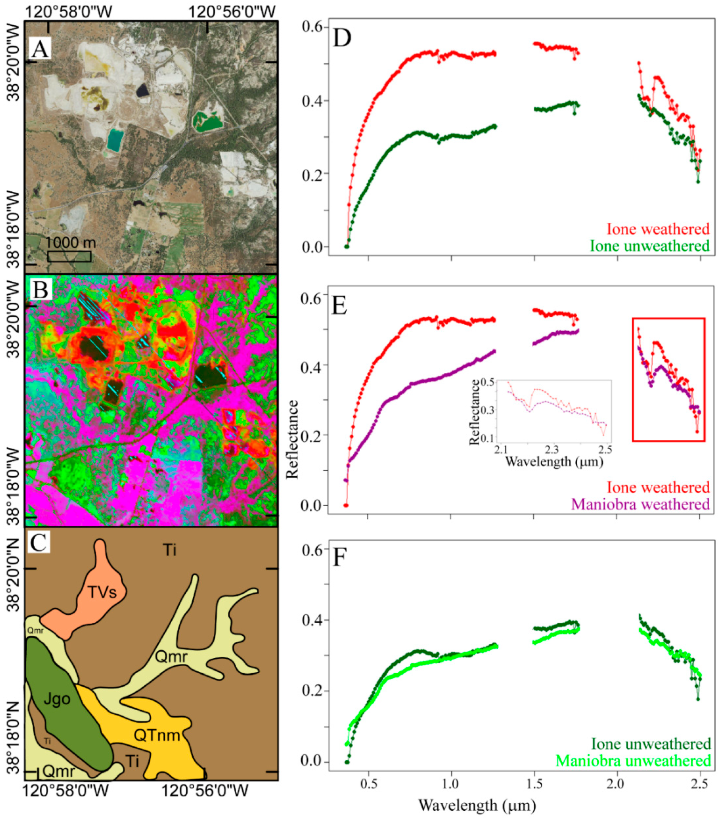
2.2. Study Sites

The three examples of the BTN presented here span a wide geographic range across central and southern California (Figure 1). Each of the sites is characterized by a paleosol horizon of in situ weathered bedrock subjacent to the BTN, depositionally overlain by Eocene and older sediments.

2.2.1. Maniobra

Near Mecca Hills, California, the Eocene Maniobra Formation sits depositionally on exhumed Mesozoic granitic basement. The Maniobra Formation consists primarily of shallow marine and nearshore submarine canyon deposits [32,33,34]. At the base of the section, a deeply weathered paleosol horizon is preserved where fractured and lightly weathered granitic rocks grade upward into deeply weathered, silicified, coarse grus deposits of the basal Maniobra formation. At this location, the BTN preserves a hillslope comprising circa 50 m of paleorelief (Figure 2A).

2.2.2. Ione

The farthest north of the sites near Ione, California hosts a deep lateritic horizon immediately below the BTN where bedrock lithology is the Jurassic Gopher Ridge volcanics [23,24,37,41]. Across roughly 10 m of bedrock, outcrops of intact metavolcanics grade upward into an increasingly weathered paleosol, marked by meter thick zones of almost complete lateritic replacement of bedrock by fine grained ferruginous material and red/orange mottled vermiform laterite (Figure 2B,C). Due to active mining operations and strictly controlled rangeland, field access to these outcrops is extremely limited and only a few field samples were obtained. The overlying shallow marine and deltaic Ione formation of Eocene age is sourced largely from deeply weathered material eroded off the upstream equivalent of the sub-BTN paleosol.

2.2.3. Goler

The Goler Formation of the El Paso Mountains, California comprises a greater than 4 km thick Paleocene and Eocene sedimentary section. The lower several kilometers consist of non-marine clastic sedimentary rocks of primarily fluvial origin, which are dated primarily by the presence of distinctive Paleocene mammalian fauna in the upper part of the section [27,29,42,43,44,45]. Preliminary magnetostratigraphy is in agreement with paleontologic age constraints [31]. Farther upsection, an Early Eocene marine incursion is recorded by the presence of fine grained marine sedimentary rocks which host a fossil foraminiferal fauna of Early Eocene age [46]. At the base of the section, more than 2 km downsection from the oldest biostratigraphic age constraint, a lateritic paleosol is preserved on Paleozoic metamorphic rocks [40]. Previous workers have generally assigned the age of the Goler Formation as Paleocene and Eocene, but have also speculated on the potential that the base of the section could represent deposition in Late Cretaceous time, e.g., [31].

3. Material and Methods

3.1. Data–AVIRIS

AVIRIS data for the Maniobra and Ione field sites were downloaded from the NASA AVIRIS Data Portal website (https://aviris.jpl.nasa.gov/alt_locator/) as Level 2 atmospherically corrected reflectance. Fortunately, the Maniobra site is located within the AVIRIS Southern California Box, so data from 17 repeat flights were available in the archive at the time of the analysis [access date 1 October 2019]. Browse images for each flight were examined. The three clearest flight lines were downloaded and flight line f130419t01p00r09 was ultimately selected on the basis of its minimal sensor noise, nearly ideal solar geometry, absence of visible atmospheric effects, and generally excellent overall data quality. The Ione site is located within the AVIRIS Tahoe Box, so data from 11 repeat flights were available. Browse images of each flight were examined and all lines with no visible cloud cover of the region of interest were downloaded and examined. Atmospheric, soil moisture, and sensor noise effects varied widely among the flight lines and f180621t01p00r08 was selected on the basis of minimizing these effects. Unfortunately, no AVIRIS data coverage was available for the Goler site. For all analyses using AVIRIS data, bands 99–121 and 149–186 were excluded on the basis of high amplitude noise likely associated with their proximity to strong atmospheric gas absorptions.

3.2. Data – Sentinel-2

Sentinel-2 data for the Goler site were downloaded as exoatmospheric reflectance (Level 1C) from the European Space Agency (ESA) Copernicus Open Access Hub (https://scihub.copernicus.eu/). A single image acquisition collected on June 28, 2018 was selected on the basis of clear atmospheric conditions and nearly optimal solar geometry. Atmospheric, topographic, and BRDF correction was performed using the SNAP Sen2Cor module [13]. A wide range of parameters was tested. The default atmospheric correction parameters yielded the most physically plausible results. Topographic and BRDF correction modules were ultimately excluded from the workflow because all parameter choices introduced undesirable image artifacts, likely as a result of the 90 m DEM required at the time of the time of analysis by the Sen2Cor package. No further correction was attempted because the favorable illumination geometry provided satisfactory image quality for the purposes of the analysis. Minor geolocation inconsistencies were observed between Sentinel-2, AVIRIS, NAIP, and published geologic map data. Correction with simple translations on the order of 1–2 pixels in x and/or y was deemed satisfactory given the purpose of the analysis.

3.3. General Approach to Analysis

3.3.1. False Color Composite Images

Mineralogical and textural differences between geologic units facilitate mapping of the contacts between those units. For a field geologist, a trained human eye remains the standard tool for making such observations. The high degree of correlation generally present in the reflectance properties of Earth materials at visible wavelengths (i.e., those shown in Google Earth) frequently results in low contrast and pernicious nonuniqueness among mineralogically distinct units both in the field and when using imagery to inform mapping decisions. These limitations can make visual identification of geologic gradients and abrupt transitions exceedingly difficult from nadir looking visible imagery, even with sub-meter spatial resolution. However, characteristic mineral absorptions are common in the near and shortwave infrared portions of the electromagnetic spectrum. False color composite images leverage an incomplete subset of this additional information by rendering multispectral data with different wavelengths of light in the Red, Green, and Blue (R/G/B) channels of the image. Additional analysis can further highlight more specific subsets of reflectance information. For geologic applications, a useful set of wavelengths is often SWIR/NIR/Visible because of the greater decorrelation in reflectance properties of common materials among these portions of the electromagnetic spectrum. For this reason, the false color composite images shown in this paper are displayed as R/G/B = SWIR 2/Broad NIR/Visible Green (i.e., Sentinel-2 bands 12, 8 and 3).

3.3.2. Linear Spectral Mixture Analysis

Mixed pixels (i.e., pixels with more than one spectrally distinct material within the ground instantaneous field of view) are common in Earth surface remote sensing. In many cases, the aggregate reflectance of a mixed pixel is well represented by an area weighted average of the reflectance of its constituent materials. Linear Spectral Mixture Analysis [47,48,49] is the quantitative application of this principle to image analysis. This approach implicitly assumes that non-linear mixing (e.g., from multiple scattering) does not contribute appreciably to the radiance upwelling into the sensor instantaneous field of view. The benefits of linear mixture models include a straightforward conceptual basis rooted in solid physical concepts and linear scaling properties (for at least some fractions) tested across meter, decameter, and hectometer spatial scales [50,51]. Mathematically, linear spectral mixture analysis can be represented by the vector equation:

$$R_{total}={\displaystyle \sum }_{i=1}^n{f}_i\times R_i+\epsilon$$

(1)

where $R_{total}$ is the observed multispectral reflectance of the mixed pixel, i represents each spectrally distinct constituent material, $R_i$ is the multispectral reflectance of material i, $f_i$ is the fractional area of the pixel covered by material i, and $\epsilon$ is model misfit. If fewer materials are modeled than the number of channels in the multispectral image, the system of equations is overdetermined and can be solved numerically using a simple constrained least squares approach. Inverting these linear mixing equations generates images representing the spatial abundance of the spectral endmembers used – based on simple fundamental physical principles. In the context of field geology, spectral mixture analysis offers substantial conceptual advantages over commonly used approaches such as spectral indices and complex machine learning methods. In contrast to spectral indices, spectral mixture analysis leverages the full information content of the reflectance spectrum, rather than a small number of bands. In contrast to machine learning, the aforementioned simple physical basis provides significant advantages in ease of computation, intuitive explanation, and obviation of overfitting. In addition, spectral mixture analysis can also be used in conjunction with more complex statistical models for specific mapping purposes.

Fractions from spectral mixture analysis are often interpreted as estimates of areal subpixel abundance. We do not strictly adopt this interpretation for this particular analysis because of the spatially extensive nature of materials not represented by either of the two endmembers present in this extremely simple model (e.g., other minerals, vegetation, soil). Instead, in this work, we interpret endmember fractions as a useful metric to estimate the spatial distribution of relative abundances of the rock types of interest for the ultimate purpose of assisting in geologic mapping. For each field site, we select endmembers derived from pixel spectra representing optimal surface exposures of the geologic materials on either side of the BTN. We then use a simple unconstrained binary linear mixture model to represent each pixel in a ~15 × 15 km area surrounding the field area as a linear mixture of these two spectra, plus misfit representing all other materials. For each field area, the outcome of this analysis is a set of images representing the Earth surface at the study site as a continuous field of relative spectral similarity to each endmember. Spatially abrupt transitions from strong spectral similarity of one endmember to the other can inform delineation of geologically significant boundaries. Each case is described in detail below.

4. Results

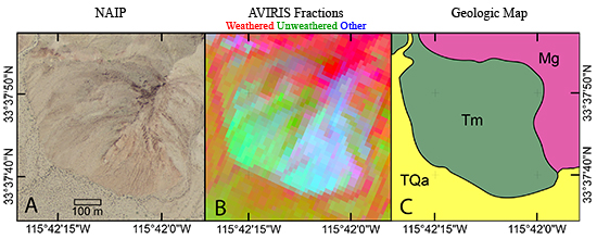
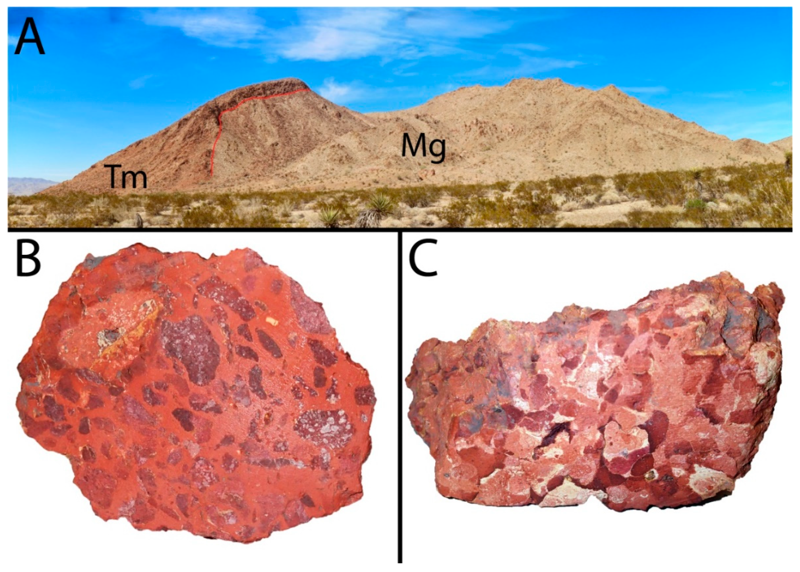
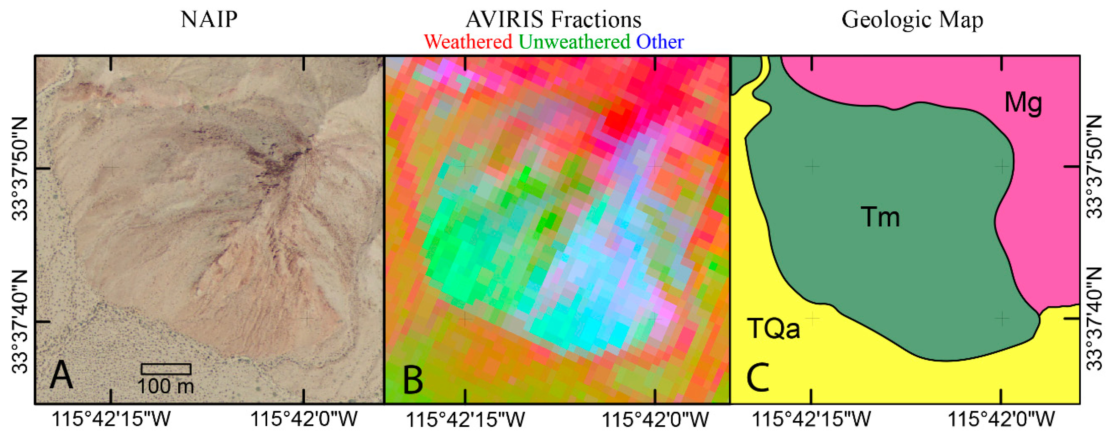
4.1. Maniobra

4.1.1. Remote Sensing Analysis

We begin our analysis with the Maniobra study site because of the generally excellent geologic exposure and availability of AVIRIS data. Figure 3 shows the Maniobra outcrop as imaged at 60 cm resolution by the 2016 National Agricultural Imagery Program (NAIP) campaign (Figure 3A). Using NAIP imagery and field photos (e.g., Figure 2A), one can visually distinguish the outcrop and associated float from the surrounding sediments and vegetation. However, discerning any internal geologic structure within the outcrop is difficult from NAIP imagery alone.

Substantially more information about spatial variability of the surface mineralogical and textural properties within the outcrop is present in the AVIRIS data (Figure 3B). Spectral endmembers chosen from AVIRIS pixels within each the weathered and unweathered units (Figure 4A) show clear differences, most prominently in the form of: (1) the presence of a strong SWIR absorption feature centered near 2200 nm in outcrops of weathered material located in both the basal Maniobra Formation and uppermost weathered basement near the nonconformity, (2) the absence of this absorption feature in outcrops of unweathered material, best expressed in the hillslope of Maniobra formation above the unconformity which is locally covered in a veneer of Quaternary alluvium (Figure 3C); and (3) differences in overall amplitude and curvature of the reflectance continuum, particularly the spectral slope at NIR wavelengths near 850 nm. Based on numerous previous studies, we interpret the ~2200 nm absorption to indicate the presence of Al-rich clays (e.g., kaolinite), an expected weathering product reported at multiple BTN outcrops and known to produce absorptions centered in this portion of the spectrum due to the structure of the Al-OH bond e.g., [17,24,25,52,53].

These differences in reflectance continua provide unambiguous features with which to discriminate the rocks at the BTN. However, in many cases hyperspectral imagery is not available and analysis must rely on multispectral spectral signatures. In order to explore how these spectral differences would be manifest by commonly used multispectral sensors, we convolve the AVIRIS spectra with the spectral response functions of the WorldView 3, Sentinel-2, and Landsat 8 instruments (Figure 4B–D). As expected, the spectral differences between the two units are less distinct for each of these multispectral sensors than for the full AVIRIS data. However, the positioning of the WorldView 3 SWIR band does result in sufficient information retention to capture the ~2200 nm absorption feature, demonstrating that the approximate depth and spectral location of this absorption could be accurately recovered from WorldView 3 multispectral observations. In addition, the NIR bands of both WorldView 3 and Sentinel-2 are able to capture some of the NIR spectral curvature differences between the two units. In contrast, the Landsat spectral bands are only able to capture the broad scale differences in overall amplitude of the spectral continuum.

We then convolve the spatial subset of the AVIRIS image data surrounding the Maniobra BTN outcrop to the spectral response functions of each sensor and unmix each simulated dataset with the corresponding simulated endmembers. Finally, we compute histograms quantifying the difference in fraction estimates between unmixing results computed for each simulated multispectral sensor and unmixing results computed with the full AVIRIS data (Figure 4E–G). WorldView 3 provides a nearly unbiased estimate with minimal dispersion (weathered and unweathered endmember mean differences = −0.02 and 0.03; standard deviations = 0.04 and 0.05, respectively). Both Sentinel-2 and Landsat 8 provide more biased estimates with substantially broader dispersion (e.g., AVIRIS - Sentinel and AVIRIS - Landsat unweathered endmember mean differences = 0.12 and 0.10; standard deviations = 0.07 and 0.08, respectively). More detailed investigation into the impacts of information loss on data dimensionality, eigenstructure, and spectral separability is included in the Appendix A (Figure A1, Figure A2 and Figure A3). Taken together, these results are encouraging for the potential application of WorldView 3 imagery for geologic applications, particularly those requiring mapping of chemical weathering intensity, demonstrating the clear utility of the additional SWIR bands over Sentinel-2 and Landsat 8 spectral capabilities. Importantly, this is true based on spectral information content alone — even without considering the superior spatial resolution of WorldView 3.

4.1.2. Geologic Interpretation of Endmember Spectra and Fraction Image

The unmixing result produces a tricolor fraction image showing spatial patterns of spectral similarity to the weathered basement endmember (Red) the unweathered basement endmember (Green) and misfit (Blue) representing all other materials in the area (Figure 3B). Geologically, the boundary between the basement and the Maniobra Formation is complex, with the basal unit of the Maniobra Formation comprised of locally derived weathered basement that is ferruginous, silicified, and likely has not been transported more than a few tens of meters [32,33,34]. In the field, this is manifest as a diffuse transition from fractured and weathered in situ basement below the unconformity upsection into locally derived silicified grus of the basal Maniobra Formation. Thus, the presence of chemical weathering products like Al-rich clays (e.g., Kaolinite) that are represented by the ~2200 nm absorption feature is expected both in the uppermost weathered basement and the lowermost Maniobra Formation. Traditional mapping methods represent this diffuse weathered zone as a sharp line with basement below and Maniobra Formation above, relegating detailed description of the true nature of the contact to a written report that accompanies a map, which often times will not be read when using the map. In this context, a spatially explicit, colorized raster representation of the BTN at this location (such as the result of this analysis) contributes to the current geological knowledge by providing a visualization of field observable data that previously was de facto overlooked by traditional geologic mapping. On the other hand, remote sensing data alone would be insufficient for understanding the geology of the area. At a minimum, the remote sensing product overlooks contributions to the signal from younger features such as slope wash, which are more accurately attributed to Quaternary processes than the structure of the original unconformity. The two methods are clearly most useful if used synergistically, a point which we will further elucidate later in the paper.

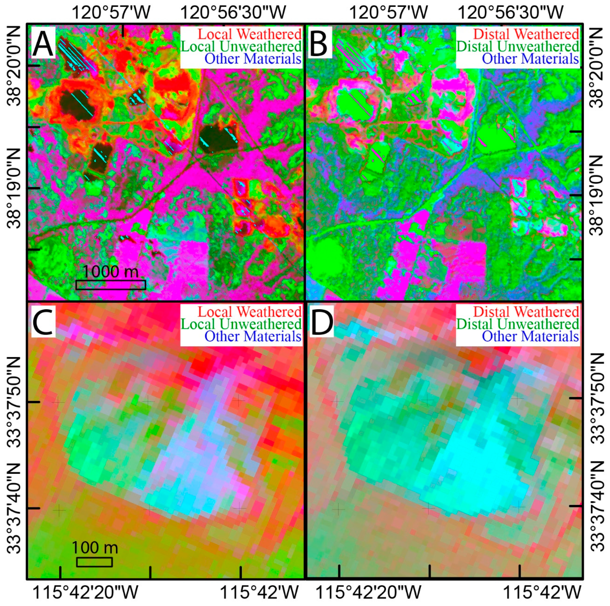
4.2. Ione

4.2.1. Remote Sensing Analysis

The Ione study area provides a substantially more complex scenario than Maniobra due to widespread anthropogenic alteration of the land surface and relatively dense vegetation cover. This complexity is evident in the 2016 NAIP imagery of the area, shown in Figure 5A. Fortunately, several large open pit mining operations are present in the study area, resulting in a set of spatially extensive and moderately homogenous reflectance targets. Using field knowledge and a published geologic map [54], we determine the location of one mine that exposes weathered material near the BTN at the base of the Ione formation and an additional outcrop where mining operations excavated deeper into less weathered exposures of the basement rocks. We then derive endmembers from pixels determined to have the best exposure within each outcrop and use these endmembers to unmix the AVIRIS data. The result is an endmember fraction image (Figure 5B) which is conceptually similar to the product generated above for the Maniobra location. This image represents spectral similarity of each pixel to the weathered endmember (Red), the unweathered endmember (Green), and RMS Misfit (Blue) which represents all other materials. In this image, geologically useful outcrops are clearly distinct from locations with extensive vegetation cover or human footprint. As at the Maniobra site, the primary spectral distinctions between the endmembers representing the weathered material (in this case the lower Ione Formation and uppermost basement) and unweathered material (in this case deeper exposures of local basement) are (1) the presence/absence of a strong SWIR absorption centered near 2200 nm, and (2) the overall spectral slope and curvature in the NIR (Figure 5C). When the weathered Ione endmember is compared directly against the weathered Maniobra endmember (Figure 5D), similarities and differences are both evident. We interpret the steeper visible and NIR spectral slope of the weathered Ione endmember as the putative result of the freshness of exposure and abundance of fine-grained comminution products resulting from its location in a mine. Interestingly, the SWIR absorption feature in the weathered Ione endmember is also broader than the absorption present in the weathered Maniobra endmember, suggestive of potentially geologically significant differences in weathering. In contrast, few prominent differences are visibly present when the unweathered spectra from the two locations are plotted together (Figure 5E).

4.2.2. Geologic Interpretation of Endmember Fraction Image and Matrix

The lower Ione Formation and subjacent basement exposures of the Jurassic Gopher Ridge volcanics are deeply chemically weathered, and the paleosol preserved at their contact (the BTN) is host to significant deposits of the Al-rich clay mineral kaolinite. This mineralogy and the associated rock textures are consistent with the reflectance spectra observed in the Ione AVIRIS data. Compared to the weathered Maniobra endmember, the ~2200 nm absorption in the weathered Ione endmember is broader, suggesting either a greater local fraction of Al-rich clay minerals and/or mineralogical differences consistent with greater severity of chemical weathering. Overall, the spectral data are in accord with published mineralogical and textural observations.

We additionally compute a 2 × 2 conceptual matrix showing the results of unmixing both sets of AVIRIS data using both pairs of endmembers (Figure 6). The purpose of this matrix is to visually evaluate the relative similarity of the BTN at two locations that are geographically distal, yet share a significant geological likeness. In both cases, local endmembers produce superior unmixing results (Figure 6A,C) but distal endmembers still produce useful spatial patterns. This similarity in unmixing results using cross-location endmembers which span nearly 1000 km strongly supports the inference suggested by earlier field-based studies of mineralogic, textural, and ultimately genetic similarity amongst the BTN outcrops at Ione and Maniobra.

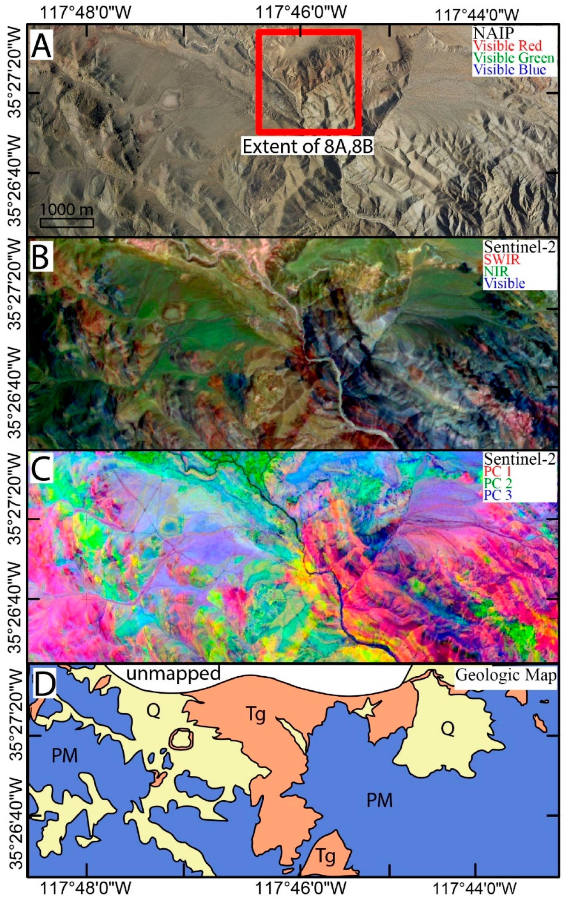
4.3. Goler

4.3.1. Remote Sensing Analysis

Our third example presents a more generally applicable case in which multispectral satellite data are available but airborne hyperspectral data are not. As at the Maniobra and Ione locations, 60 cm resolution aerial imaging at visible wavelengths (Figure 7A) provides limited ability to discriminate between the Goler formation and the underlying basement. Substantially more information is provided in a false color composite image using Sentinel-2 data (Figure 7B; R/G/B = SWIR/NIR/Vis). Applying a Principal Component transformation to the same Sentinel-2 image (Figure 7C) compresses even more information into a single tricolor image, showing clear spatially coherent patterns consistent with expected mineralogical and textural differences spatially distributed across geologic units within the field site.

We then unmix Sentinel-2 data using both the Maniobra AVIRIS endmembers resampled to Sentinel-2 spectral resolution (Figure 8A) and local Sentinel-2 spectral endmembers derived from pixels with unobstructed exposure of the Goler and underlying basement units of the El Paso terrane ([55]; Figure 8B). As in the case of the comparative matrix (Figure 6), both unmixing products provide useful geologic information but local endmembers are clearly better suited to assist geologic mapping.

4.3.2. Geologic Interpretation of Endmember Fraction Image

Because hyperspectral data is unavailable for most of the globe, there is a significant geological utility to testing the application of this method to a location where only multispectral data is available. At the Goler site a lateritic horizon is present at the BTN and the overlying basal Goler Formation is largely composed of weathered sediments derived from the local basement rocks. The successful representation of the BTN achieved by applying the Maniobra endmembers to Goler Sentinel 2 data is independent evidence supporting the inference of clear geological similarities reported amongst the three study sites. Additionally, at the Goler location, the subjacent basement rocks are primarily Permo-Triassic metasediments, which preserve a significant amount of internal structure such as bedding planes. These structures are represented quite clearly in both Figure 7B (false color) and Figure 7C (principal component rotation), which closely match the published bedrock mapping of the area [56] (Figure 7D).

5. Discussion

The basal Tertiary nonconformity in the southwest U.S. is an important datum for tracking Cenozoic tectonics, exhumation, and sedimentation. Previous studies have characterized the nonconformity using traditional geological tools such as field mapping, petrology, and geochemistry. These studies document a unique set of outcrops at the base of the Tertiary section across the region, nearly ubiquitously including deep chemical weathering of the bedrock subjacent to the BTN. For the first time here, we use remote sensing tools to independently characterize the reflectance properties of these outcrops, and also evaluate the mineralogic and lithologic similarity at each site.

Minerals produced by chemical weathering and hydrothermal alteration often have distinctive VSWIR reflectance signature [57,58,59,60,61]. At the sites presented here, confirming and constraining the spatial distribution of these minerals is a significant complement to field observations because the abundance of these minerals provides an accurate (insofar as the ground surface is representative of the underlying bedrock), independent, physically-based representation of the complexity of the spatial pattern of chemical weathering on a pixel-by-pixel basis without regard for limitations and decisions required to make a geologic map from field data. Importantly for the general case, this is true even if the specific mineral causing the absorption cannot easily be identified. In the case of the Maniobra site, we know from field mapping that the bedrock immediately subjacent to the BTN is primarily composed of in situ chemically weathered felsic plutonic rock. On the other hand, the lowermost Maniobra Formation is characterized by a similar lithology of chemically weathered felsic plutonic rock—except rather than being truly in situ, it is composed of locally-derived sediments, which are pieces of local weathered basement. This geologic contact presents a challenge for traditional field mapping because the continuous nature of the boundary makes it difficult to represent accurately as a single line on map. To date, the result of this continuous mapping dilemma been a simplified map representation of the contact as a single line drawn somewhere within the weathered material, with a more rigorous description of the contact left for a textual description. Our raster-based spectral unmixing result using the two endmembers defined by a “less weathered” and “more weathered” approximation fundamentally contributes a new perspective and visualization of the geologic interpretation made by previous workers at this site. By imaging this alteration, we constrain the location and sharpness of the basal unconformity with a level of precision and accuracy that is not attainable through field observations or high spatial resolution visible imagery alone. While the presence of the specific ~2200 nm absorption and availability of airborne hyperspectral imaging facilitates this process at this particular location, the methodology is general. The approach presented here could easily be adapted for comparable geologic mapping purposes anywhere – provided that the variations of interest in surficial weathering, mineralogy, lithology, and/or texture generate VSWIR absorption features which are sufficiently distinct to be resolved by the multispectral or hyperspectral data available to the mapper.

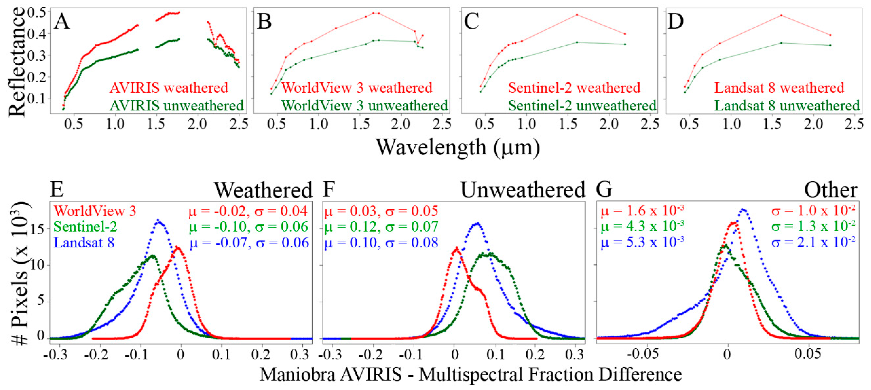
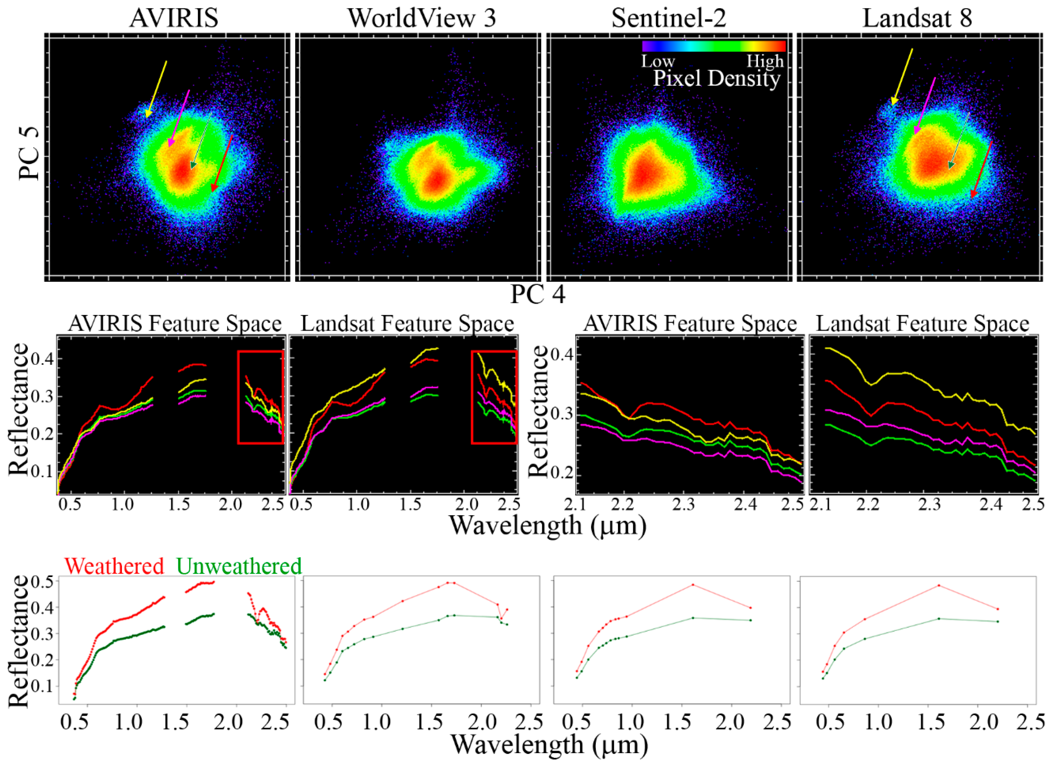
5.1. Impact of Sensor Spectral Resolution

Resampling the Maniobra AVIRIS endmembers to the spectral resolution of WorldView 3, Sentinel-2 and Landsat 8 provides considerable insight into the capabilities and limitations of each multispectral sensor, as well as a compelling illustration of the value of a hyperspectral sensor which is able to sample the full VSWIR spectral continuum. The ability of the WorldView 3 SWIR bands to capture the ~2200 nm absorption found in the AVIRIS data resulted in the retention of considerably more information than is captured by the Sentinel-2 or Landsat 8 spectra. This increased spectral information clearly results in enhanced clustering in the feature space — directly implying more unambiguous statistical separability and ultimately superior utility for geologic mapping. Notably, this information persists despite the spectral gaps among the bands of WorldView 3 and their 30 to 70 nm spectral widths. Combined with the capability to image at 7.5/3.7 m spatial resolution, this result provides compelling evidence for the potential application of WorldView 3 data to geologic problems similar to those considered in this study.

However, despite the loss of the ~2200 nm absorption and the associated data dimensionality and spectral separability, both Sentinel-2 and Landsat 8 successfully resolved sufficient differences in the spectral continuum to yield false color composite, principal component, and fraction images with unambiguously superior contrast than the visible-band NAIP imagery. The additional spectral information contributed by the relatively broad Sentinel-2 and Landsat 8 NIR and SWIR bands suggests that sufficient spectral information is present in multispectral sampling of the continuum to enable the decameter spatial resolution Sentinel-2 and Landsat 8 to usefully complement visible imagery with high spatial resolution. Viewed together, these results suggest that an optimized approach to geologic mapping in the absence of hyperspectral aerial imaging will use multispectral satellite imagery in concert with higher spatial resolution imagery to take advantage of both the spectral and spatial resolutions of the multisensor suite of observations.

5.2. Sentinel-2 at the Goler Site

Because of the absence of AVIRIS coverage, the analysis of the Goler field site is the most general and broadly applicable of the locations considered in this work. In this case, unmixing with local endmembers provides substantially greater insight than unmixing with Maniobra endmembers. Surprisingly, the unmixing result using local endmembers effectively distinguishes the basal unit of the Goler Formation from all other nearby lithologies, including bedrock, alluvium, and other members of the Goler Formation. This basal unit is composed primarily of deeply weathered clasts derived from local basement rocks. Differences exist among the spectra of the basal Goler and of other local lithologies, even at Sentinel-2 spectral resolution (Figure 9). These differences can be understood – and quantified – in terms of spectral slope in both VNIR and SWIR portions of the spectrum, overall amplitude of the reflectance, and presence/absence of a difference in reflectance between the narrow and broad NIR channels of the Sentinel-2 sensor (bands 8 and 8a), consistent with the potential capture of an aliased signal from weak NIR absorptions near 850 nm. Such a signal is consistent with the quasi-bilinear behavior near 850 nm prominent in the hyperspectral AVIRIS endmember from the Maniobra location (Figure 4) and less obviously in the AVIRIS endmember from the Ione location (Figure 5).

The relative utility of local versus distal endmembers raises the question of the potential that further insight might be provided in some cases by globally standardized mixture models. Endmembers that bound the global mixing space have been identified and intercalibrated for the Landsat 4–8 and Sentinel-2 sensors (e.g., [50,51,62,63]). Unmixing image data of the Maniobra and Goler field sites using the endmembers bounding the global space yields fraction estimates which generally fall near the Substrate to Dark binary mixing continuum, as expected given the low density of vegetation in these locations. While global endmember fractions by themselves clearly do not yield accurate estimates for the purposes of this analysis, variations in the misfit and spectral residual associate with the global model do show geologically suggestive spatial patterns. It is possible that the information in misfit and spectral residual might be used in future studies to provide a more standardized approach for the characterization and mapping of rocks and soils. California might be an ideal landscape for such a study due to the diversity of rocks and soils, and associated spectral complexity, which has been shown to reasonably approximate the global feature space [64].

5.3. Using Reflectance to Map Geologic Contacts

For each of the field sites, the spectral information present in the decameter resolution clearly adds a complementary perspective to the NAIP imagery with sub-meter resolution but highly correlated spectral bands. This information allows us to identify major unit boundaries present on the bedrock geologic map with considerably more confidence than using visible imagery alone. Additionally, sub-unit variations within individual map units are distinguishable on a more detailed scale than is shown on the field mapping scale. Detailed lithologic descriptions that accompany geologic maps often include written documentation of this type of more detailed variation within a single map unit. In this case, we see two major benefits to including this type of remote sensing data in the workflow and presentation of a geologic map. On one hand, the mapper will be able to better describe the rocks on the ground if he uses this data before, during, and after field work. On the other hand, the map reader is given a major benefit by being able to visualize the variability in the imagery alongside a written description versus a written description alone.

5.4. Mapping Geologic Units across A Gradational Contact

As stated previously, remote sensing data can quantify geologically relevant gradients. At the BTN outcrop at the base of the Maniobra Formation, clear spectral differences exist between two geologic map units identified as Mesozoic felsic granitoid basement (Mg) and Tertiary Maniobra Formation (Tm). Detailed published work describes the geologic contact between these two units as a nonconformity characterized by deeply weathered in situ Mg beneath the BTN grading upward into locally derived, but not strictly in situ sediments composed almost entirely of the same material from beneath the unconformity. Because of this relationship, this nonconformity approximates a gradational contact, despite representing a very long period of non-deposition and a large magnitude of exhumation. Representative weathered and unweathered spectra show considerable differences in (a) the depth of the absorption centered near 2200 nm, (b) the spectral slope between the NIR and SWIR1 bands, and (c) the spectral slope between the visible bands and the NIR bands (Figure 3). The observed differences between these spectra are consistent with distinctive combinations of absorptions generated by the mineral assemblages and textures which comprise the bedrock units, particularly as characterized by a difference in overall extent of weathering between the units.

5.5. Global Implications for Geologic Mapping

Despite the free availability of global multispectral optical remote sensing observations via the Landsat and Sentinel programs and the clear utility these data provide for geologic interpretation, these data have not attained widespread utilization as a part of geologic mapping workflows. The analyses presented here provide a suite of both qualitative and quantitative examples to demonstrate how integrating multispectral false color composite images, principal component images, and simple linear mixture models can aid in the generation and interpretation of geologic maps.

In some ways the interpretative framework described in this study does closely mimic the process of field data collection and interpretation that a geologist undertakes in the process of creating a map. For example, traditional methods to document and quantify intraunit variability are standard tools for field workers. But the amount of time and effort required to implement these methods requires that they be only implemented locally and then extrapolated over large areas, if they are used at all. Remote sensing data augments the mapping process and allow quantitative observations to be made more easily at the scale of an entire map area. These tools provide new benefits for both the mapper and the map user.

The tools presented here contribute analytical products derived from rigorously intercalibrated, spatially explicit, quantitative observations on spatial scales that are larger than are typically practical for detailed field studies. While our results show clear benefits to the inclusion of multispectral imagery in the workflow of geologists, accurate geological interpretation – and ultimately understanding – fundamentally relies on detailed field observations. Multispectral and hyperspectral imagery has the potential to greatly assist in the direction of field campaigns, extrapolation of those observations across areas unable to be visited in the field, and quantification of physical parameters. However, we emphasize that this type of remote sensing analysis should be seen as a supplement to – not a replacement for – primary field data collection and interpretation.

6. Conclusions

Geologic maps provide fundamental constraints on the spatial extent and orientation of earth materials and structures. The ongoing technical evolution of remote sensing data products has significantly expanded the scope of available information to a mapper. For workers from governmental agencies, private industry, and academia alike, the information contained in geologic maps can be enhanced by integrating data from remote sensing products.

In an exploration of elements that transcend traditional boundaries between field geology and optical remote sensing, we present a study of the basal Tertiary nonconformity in California. The similarities and differences among AVIRIS-measured VSWIR reflectance spectra from two of these three sites and their neighboring basement inform our understanding of their similarity. This understanding is then extended to the third site where only multispectral Sentinel-2 observations are available. The principal conclusions and implications of this study are:

(1)

the information available about the location and depth and individual absorptions present in the hyperspectral AVIRIS data provides novel information which can be incorporated in geologic map descriptions with substantial greater specificity than field observations alone;

(2)

the information present in the spectral continuum captured by Sentinel-2 and Landsat 8 allows for general discrimination of geologic map units across the unconformity of interest, but results in the loss of important spatial variations in strength of the ~2200 nm absorption;

(3)

in contrast, the ~2200 nm absorption is successfully captured by the WorldView 3 SWIR bands, with unambiguous feature space clustering, statistical separability, and ultimately geologic mapping utility;

(4)

linear spectral unmixing using both local and distal spectral endmembers can greatly assist in both delineating boundaries between geologic units and visualizing continuous field gradients;

(5)

a comprehensive field campaign ultimately benefits most from using decameter spectral information in concert with both the detailed spatial information present in sub-meter resolution air photos or satellite imagery.

References

- Saleeby, J.; Saleeby, Z.; Sousa, F. From deep to modern time along the western Sierra Nevada foothills of California, San Joaquin to Kern River drainages. Geol. Soc. Am. Field Guides 2013, 32, 37–62. [Google Scholar]
- Sousa, F.J.; Saleeby, J.; Farley, K.A.; Unruh, J.R.; Lloyd, M.K. The southern Sierra Nevada pediment, central California. Geosphere 2017, 13, 82–101. [Google Scholar] [CrossRef]
- Van Buer, N.J.; Miller, E.L.; Dumitru, T.A. Early Tertiary paleogeologic map of the northern Sierra Nevada batholith and the northwestern basin and range. Geology 2009, 37, 371–374. [Google Scholar] [CrossRef]
- Sousa, F.; Saleeby, J.; Farley, K.A. Chronology of tectonic and landscape evolution of the southern Sierra Nevada foothills-eastern San Joaquin basin transition, CA. In Pacific Section AAPG, SPE and SEPM Joint Technical Conference; American Association of Petroleum Geologists: Bakersfield, CA, USA, 2014. [Google Scholar]
- Sousa, F.J. Eocene origin of Owens Valley, California. Geosciences 2019, 9, 194. [Google Scholar] [CrossRef]
- Sousa, F.; Saleeby, J.; Farley, K.A.; Unruh, J. The southern Sierra Nevada foothills bedrock pediment. In 2013 GSA Cordilleran Section Meeting; GSA Abstracts with Programs: Fresno, CA, USA, 2013; Volume 45, p. 53. [Google Scholar]
- Wulder, M.A.; Masek, J.G.; Cohen, W.B.; Loveland, T.R.; Woodcock, C.E. Opening the archive: How free data has enabled the science and monitoring promise of landsat. Remote Sens. Environ. 2012, 122, 2–10. [Google Scholar] [CrossRef]
- Markham, B.L.; Helder, D.L. Forty-year calibrated record of earth-reflected radiance from Landsat: A review. Remote Sens. Environ. 2012, 122, 30–40. [Google Scholar] [CrossRef] [Green Version]
- Claverie, M.; Ju, J.; Masek, J.G.; Dungan, J.L.; Vermote, E.F.; Roger, J.C.; Skakun, S.V.; Justice, C. The Harmonized Landsat and Sentinel-2 surface reflectance data set. Remote Sens. Environ. 2018, 219, 145–161. [Google Scholar] [CrossRef]
- Storey, J.; Choate, M.; Lee, K. Landsat 8 Operational Land Imager on-orbit geometric calibration and performance. Remote Sens. 2014, 6, 11127–11152. [Google Scholar] [CrossRef]
- Masek, J.G. Landsat Ecosystem Disturbance Adaptive Processing System (LEDAPS); NASA: Washington, DC, USA, 2006; p. 1.
- Vermote, E.; Roger, J.C.; Franch, B.; Skakun, S. LaSRC (Land Surface Reflectance Code): Overview, application and validation using MODIS, VIIRS, Landsat and Sentinel 2 data. In Proceedings of the IGARSS 2018–2018 IEEE International Geoscience and Remote Sensing Symposium, Valencia, Spain, 22–27 July 2018; pp. 8173–8176. [Google Scholar]
- Mueller-Wilm, U.; Devignot, O.; Pessiot, L. S2 MPC Sen2Cor Configuration and User Manual; European Space Agency: Paris, France, 2017; Available online: https://step.esa.int/thirdparties/sen2cor/2.4.0/Sen2Cor_240_Documenation_PDF/S2-PDGS-MPC-L2A-SUM-V2.4.0.pdf (accessed on 26 October 2019).
- Kruse, F.A. The Effects of Spatial Resolution, Spectral Resolution, and SNR on Geologic Mapping Using Hyperspectral Data, Northern Grapevine Mountains, Nevada. In Proceedings of the AVIRIS Airborne Geoscience Workshop; Northern Grapevine Mountains: Pasadena, CA, USA, 2000. Available online: https://aviris.jpl.nasa.gov/proceedings/ (accessed on 26 October 2019).
- Calvin, W.M.; Pace, E.L. Utilizing HyspIRI prototype data for geological exploration applications: A southern California case study. Geosciences 2016, 6, 11. [Google Scholar] [CrossRef]
- Witkosky, R.D.; Adams, P.; Akciz, S.; Buckland, K.; Harvey, J.; Johnson, P.; Lynch, D.K.; Sousa, F.; Stock, J.; Tratt, D. Geologic swath map of the Lavic Lake fault from airborne thermal hyperspectral imagery. In Proceedings of the 2016 8th Workshop on Hyperspectral Image and Signal Processing: Evolution in Remote Sensing (WHISPERS), Los Angeles, CA, USA, 21–24 August 2016; pp. 1–5. [Google Scholar]
- Kruse, F.A.; Boardman, J.W.; Huntington, J.F. Comparison of airborne hyperspectral data and EO-1 Hyperion for mineral mapping. IEEE Trans. Geosci. Remote Sens. 2003, 41, 1388–1400. [Google Scholar] [CrossRef]
- Lewis, M.D.; Gould, R.W.; Arnone, R.A.; Lyon, P.E.; Martinolich, P.M.; Vaughan, R.; Lawson, A.; Scardino, T.; Hou, W.; Snyder, W.; et al. The Hyperspectral Imager for the Coastal Ocean (HICO): Sensor and Data Processing Overview; OCEANS 2009; IEEE: Biloxi, MS, USA, 2009; pp. 1–9. [Google Scholar]
- Lindgren, W. The Tertiary Gravels of the Sierra Nevada of California; U.S. Geological Survey Professional Paper 73; United States Government Printing Office: Washington, DC, USA, 1911.
- Saleeby, J.; Farley, K.A.; Kistler, R.W.; Fleck, R.J. Thermal evolution and exhumation of deep-level batholithic exposures, southernmost Sierra Nevada, California. Spec. Pap. Geol. Soc. Am. 2007, 419, 39–66. [Google Scholar]
- Chapman, A.D.; Saleeby, J.; Wood, D.J.; Piasecki, A.; Kidder, S.; Ducea, M.N.; Farley, K.A. Late Cretaceous gravitational collapse of the southern Sierra Nevada batholith, California. Geosphere 2012, 8, 314–341. [Google Scholar] [CrossRef]
- Wood, D.J.; Saleeby, J.B. Late Cretaceous-Paleocene extensional collapse and disaggregation of the southernmost Sierra Nevada batholith. Int. Geol. Rev. 1997, 39, 973–1009. [Google Scholar] [CrossRef]
- Allen, V.T. The Ione Formation of California. Univ. Calif. Publ. Geol. Sci. 1929, 18, 347–448. [Google Scholar]
- Bates, T.F. Origin of the Edwin clay, Ione, California. Geol. Soc. Am. Bull. 1945, 56, 1–38. [Google Scholar] [CrossRef]
- Wood, J.L. A Re-Evaluation of the Origin of Kaolinite in the Ione Depositional System (Eocene), Sierra Foothills, California; UCLA: Los Angeles, CA, USA, 1994. [Google Scholar]
- Saleeby, J.; Saleeby, Z.; Robbins, J.; Gillespie, J. Sediment provenance and dispersal of nNogene–Quaternary strata of the southeastern San Joaquin basin and its transition into the southern Sierra Nevada, California. Geosphere 2016, 12, 1744–1773. [Google Scholar] [CrossRef]
- Cox, B. Stratigraphy, Sedimentology, and Structure of the Goler Formation (Paleocene), El Paso Mountains, California: Implications for Paleogene Tectonism on the Garlock Fault Zone; University of California: Riverside, CA, USA, 1982. [Google Scholar]
- Cox, B.F.; Diggles, M. Geologic Map of the El Paso Mountains Wilderness Study Area, Kern County, California; United States Geological Survey Miscellaneous Field Studies Map 1827; 1986. Available online: https://pubs.er.usgs.gov/publication/mf1827 (accessed on 26 October 2019).
- Cox, B. Stratigraphy, depositional environments, and paleotectonics of the Paleocene and Eocene Goler Formation, El Paso Mountains, California: Geologic summary and roadlog. In Basin Analysis and Paleontology of the Paleocene and Eocene Goler Formation, El Paso Mountains, California; Society of Economic Paleontologists and Mineralogists: Los Angeles, CA, USA, 1987; Volume 57, pp. 1–29. [Google Scholar]
- Lechler, A.R.; Niemi, N.A. Sedimentologic and isotopic constraints on the paleogene paleogeography and paleotopography of the southern Sierra Nevada, California. Geology 2011, 39, 379–382. [Google Scholar] [CrossRef]
- Sousa, F.J. Tectonics of Central and Eastern California, Late Cretaceous to Modern; California Institute of Technology: Pasadena, CA, USA, 2016. [Google Scholar]
- Crowell, J.C.; Susuki, T. Eocene stratigraphy and paleontology, Orocopia Mountains, southeastern California. Geol. Soc. Am. Bull. 1959, 70, 581–592. [Google Scholar] [CrossRef]
- Advocate, D.M.; Link, M.H.; Squires, R.L. Anatomy and history of an Eocene submarine canyon: The Maniobra Formation, Southern California. In Paleogene Stratigraphy, West Coast of North America; Filewicz, M.V., Squires, R.L., Eds.; Pacific Section, Society of Economic Paleontologists and Mineralogists: Tulsa, OK, USA, 1988; pp. 45–58. [Google Scholar]
- Caracciolo, L.; Arribas, J.; Ingersoll, R.V.; Critelli, S. The diagenetic destruction of porosity in plutoniclastic petrofacies: The Miocene Diligencia and Eocene Maniobra Formations, Orocopia Mountains, southern California, USA. Geol. Soc. Lond. Spec. Publ. 2014, 386, 49–62. [Google Scholar] [CrossRef]
- Pask, J.A.; Turner, M.D. Geology and ceramic properties of the Ione Formation, Buena Vista area, Amador County, California. Spec. Rep. Calif. Div. Mines Geol. 1952, 19, 1–39. [Google Scholar]
- Palmer, C. Stratigraphy, Petrology, and Depositional Environments of the Ione Formation in Madera County; CSU Fresno: Fresno, CA, USA, 1978. [Google Scholar]
- Creely, S.; Force, E.R. Type Region of the Ione Formation (Eocene), Central California; Stratigraphy, Paleogeography, and Relation to Auriferous Gravels; U.S. Geological Survey: Reston, VA, USA, 2007; p. 65.
- Sousa, F.; Saleeby, J.; Farley, K.A. (U-Th)/He chronometry of multiple secondary minerals, Sierra Nevada, California. In Goldschmidt Abstracts; Geochemical Society: Sacramento, CA, USA, 2014; p. 2358. [Google Scholar]
- Chapman, A.D.; Wood, D.J.; Saleeby, J.B.; Saleeby, Z. Late Cretaceous to early Neogene tectonic development of the southern Sierra Nevada region, California. In Field Excursions in Southern California: Field Guides to the 2016 GSA Cordilleran Section Meeting; Geological Society of America: Boulder, CO, USA, 2017; Volume 45, pp. 187–228. [Google Scholar]
- Cox, B. Early Paleogene Laterite and Debris-Flow Deposits, El Paso Mountains, California; Geological Society of America Abstracts with Programs; Geological Society of America: Boulder, CO, USA, 1979; Volume 11, pp. 73–74. [Google Scholar]
- Yapp, C.J. Fe (CO3) OH in goethite from a mid-latitude North American oxisol: Estimate of atmospheric CO2 concentration in the early Eocene Climatic optimum. Geochim. Cosmochim. Acta 2004, 68, 935–947. [Google Scholar] [CrossRef]
- McKenna, M.C.; Hutchison, J.H.; Hartman, J.H. Paleocene Vertebrates and Nonmarine Mollusca from the Goler Formation, California. In Basin analysis and paleontology of the Paleocene and Eocene Goler Formation, El Paso Mountains, California; Pacific Section of the Society of Economic Paleontologist; Cox, B.F., Ed.; AAPG: Los Angeles, CA, USA, 1987. [Google Scholar]
- Lofgren, D.; Silver, B.; Hinkle, T.; Ali-Khan, F.; Reynolds, R.; Miller, D. New marine sites from member 4d of the Goler Formation of California. Overboard Mojave 2010, 20, 232–240. [Google Scholar]
- Lofgren, D.; Mckenna, M.; Honey, J.; Nydam, R.; Wheaton, C.; Yokote, B.; Henn, L.; Hanlon, W.; Manning, S.; Mcgee, C. New records of eutherian mammals from the Goler Formation (Tiffanian, Paleocene) of california and their biostratigraphic and paleobiogeographic implications. Am. Mus. Novit. 2014, 3797, 1–57. [Google Scholar] [CrossRef]
- Albright, L.; Lofgren, D.; McKenna, M. Magnetostratigraphy, mammalian biostratigraphy, and refined age assessment of the Goler Formation (Paleocene), California. In Papers on Geology, Vertebrate Paleontology, and Biostratigraphy in Honor of Michael O. Woodburne; Museum of Northern Arizona: Flagstaff, AR, USA, 2009; Volume 65, pp. 259–278. [Google Scholar]
- McDougall, K. Foraminiferal Biostratigraphy and Paleoecology of Marine Deposits, Goler Formation, California. 1987. Available online: http://archives.datapages.com/data/pac_sepm/074/074001/pdfs/43.htm (accessed on 26 October 2019).
- Adams, J.B.; Smith, M.O.; Johnson, P.E. Spectral mixture modeling—A new analysis of rock and soil types at the Viking lander-1 site. J. Geophys. Res. Solid Earth Planets 1986, 91, 8098–8112. [Google Scholar] [CrossRef]
- Smith, M.O.; Ustin, S.L.; Adams, J.B.; Gillespie, A.R. Vegetation in deserts: I. A regional measure of abundance from multispectral images. Remote Sens. Environ. 1990, 31, 1–26. [Google Scholar] [CrossRef]
- Gillespie, A.R.; Smith, M.O.; Adams, J.B.; Willis, S.C.; Fischer, A.F.I.; Sabol, D.E. Interpretation of Residual Images: Spectral Mixture Analysis of AVIRIS Images, Owens Valley, California; Proceedings of the AVIRIS Airborne Geoscience Workshop; Pasadena, CA, USA, 1990. Available online: https://aviris.jpl.nasa.gov/proceedings/ (accessed on 26 October 2019).
- Small, C.; Milesi, C. Multi-scale standardized spectral mixture models. Remote Sens. Environ. 2013, 136, 442–454. [Google Scholar] [CrossRef] [Green Version]
- Sousa, D.; Small, C. Globally standardized MODIS spectral mixture models. Remote Sens. Lett. 2019, 10, 1018–1027. [Google Scholar] [CrossRef]
- Percival, H.J.; Duncan, J.F.; Foster, P.K. Interpretation of the kaolinite-mullite reaction sequence from infrared absorption spectra. J. Am. Ceram. Soc. 1974, 57, 57–61. [Google Scholar] [CrossRef]
- Guatame-García, A.; Buxton, M.; Deon, F.; Lievens, C.; Hecker, C. Toward an on-line characterization of kaolin calcination process using short-wave infrared spectroscopy. Miner. Process. Extr. Metall. Rev. 2018, 39, 420–431. [Google Scholar] [CrossRef] [Green Version]
- Wagner, D.L.; Jennings, C.W.; Bedrossian, T.L.; Bortugno, E.J. Geologic Map of the Sacramento Quadrangle, California, 1,250,000; California Division of Mines and Geology: Sacramento, CA, USA, 1981. [Google Scholar]
- Cecil, M.R.; Ferrer, M.A.; Riggs, N.R.; Marsaglia, K.; Kylander-Clark, A.; Ducea, M.N.; Stone, P. Early arc development recorded in Permian–Triassic plutons of the northern Mojave Desert region, California, USA. GSA Bull. 2018, 131, 749–765. [Google Scholar] [CrossRef]
- Carr, M.D.; Christiansen, R.L.; Poole, F.G.; Goodge, J.W. Bedrock Geologic Map of the El Paso Mountains in the Garlack and El Paso Peaks 7-1/2’ Quadrangle, Kern County, California; United States Geological Survey IMAP no. 2389; U.S. Department of the Interior: Newton, MA, USA, 1997.
- Galvão, L.S.; Formaggio, A.R.; Couto, E.G.; Roberts, D.A. Relationships between the mineralogical and chemical composition of tropical soils and topography from hyperspectral remote sensing data. ISPRS J. Photogramm. Remote Sens. 2008, 63, 259–271. [Google Scholar] [CrossRef]
- Crowley, J.K. Mapping playa evaporite minerals with AVIRIS data: A first report from Death Valley, california. Remote Sens. Environ. 1993, 44, 337–356. [Google Scholar] [CrossRef]
- Mohanty, B.; Gupta, A.; Das, B.S. Estimation of weathering indices using spectral reflectance over visible to mid-infrared region. Geoderma 2016, 266, 111–119. [Google Scholar] [CrossRef]
- Duncan, W.R.; Ledger, E.B.; Whitehead, V.S. X-ray diffraction verification of AVIRIS clay mineral identification, Summitville area, southwestern Colorado; NASA Jet Propulsion Laboratory: Pasadena, CA, USA, 1998; Volume 1.
- Younis, M.T.; Gilabert, M.A.; Melia, J.; Bastida, J. Weathering process effects on spectral reflectance of rocks in a semi-arid environment. Int. J. Remote Sens. 2010, 18, 3361–3377. [Google Scholar] [CrossRef]
- Small, C. The Landsat ETM+ spectral mixing space. Remote Sens. Environ. 2004, 93, 1–17. [Google Scholar] [CrossRef]
- Sousa, D.; Small, C. Global cross-calibration of Landsat spectral mixture models. Remote Sens. Environ. 2017, 192, 139–149. [Google Scholar] [CrossRef] [Green Version]
- Sousa, D.; Small, C. Multisensor analysis of spectral dimensionality and soil diversity in the great central valley of California. Sensors 2018, 18, 583. [Google Scholar] [CrossRef]
© 2019 by the authors. Licensee MDPI, Basel, Switzerland. This article is an open access article distributed under the terms and conditions of the Creative Commons Attribution (CC BY) license (http://creativecommons.org/licenses/by/4.0/).
Share and Cite
Sousa, F.J.; Sousa, D.J. Spatial Patterns of Chemical Weathering at the Basal Tertiary Nonconformity in California from Multispectral and Hyperspectral Optical Remote Sensing. Remote Sens. 2019, 11, 2528. https://0-doi-org.brum.beds.ac.uk/10.3390/rs11212528
Sousa FJ, Sousa DJ. Spatial Patterns of Chemical Weathering at the Basal Tertiary Nonconformity in California from Multispectral and Hyperspectral Optical Remote Sensing. Remote Sensing. 2019; 11(21):2528. https://0-doi-org.brum.beds.ac.uk/10.3390/rs11212528
Chicago/Turabian StyleSousa, Francis J., and Daniel J. Sousa. 2019. "Spatial Patterns of Chemical Weathering at the Basal Tertiary Nonconformity in California from Multispectral and Hyperspectral Optical Remote Sensing" Remote Sensing 11, no. 21: 2528. https://0-doi-org.brum.beds.ac.uk/10.3390/rs11212528