Assessment of the Impacts of Image Signal-to-Noise Ratios in Impervious Surface Mapping


1
U.S. Geological Survey (USGS) Earth Resources Observation and Science Center (EROS), Sioux Falls, SD 57198, USA
2
ASRC Federal Data Solutions (AFDS), Contractor to the USGS EROS, Sioux Falls, SD 57198, USA
3
USGS Land Imaging Program, Flagstaff, AZ 86001, USA
*
Author to whom correspondence should be addressed.
Remote Sens. 2019, 11(22), 2603; https://0-doi-org.brum.beds.ac.uk/10.3390/rs11222603
Submission received: 11 September 2019
/
Revised: 31 October 2019
/
Accepted: 2 November 2019
/
Published: 6 November 2019
(This article belongs to the Special Issue Advancements in Remote Sensing of Land Surface Change)
Abstract
:Medium spatial resolution satellite images are frequently used to characterize thematic land cover and a continuous field at both regional and global scales. However, high spatial resolution remote sensing data can provide details in landscape structures, especially in the urban environment. With upgrades to spatial resolution and spectral coverage for many satellite sensors, the impact of the signal-to-noise ratio (SNR) in characterizing a landscape with highly heterogeneous features at the sub-pixel level is still uncertain. This study used WorldView-3 (WV3) images as a basis to evaluate the impacts of SNR on mapping a fractional developed impervious surface area (ISA). The point spread function (PSF) from the Landsat 8 Operational Land Imager (OLI) was used to resample the WV3 images to three different resolutions: 10 m, 20 m, and 30 m. Noise was then added to the resampled WV3 images to simulate different fractional levels of OLI SNRs. Furthermore, regression tree algorithms were incorporated into these images to estimate the ISA at different spatial scales. The study results showed that the total areal estimate could be improved by about 1% and 0.4% at 10-m spatial resolutions in our two study areas when the SNR changes from half to twice that of the Landsat OLI SNR level. Such improvement is more obvious in the high imperviousness ranges. The root-mean-square-error of ISA estimates using images that have twice and two-thirds the SNRs of OLI varied consistently from high to low when spatial resolutions changed from 10 m to 20 m. The increase of SNR, however, did not improve the overall performance of ISA estimates at 30 m.

1. Introduction
The ability to continuously monitor land cover and land use conditions and change from satellite imagery is an ongoing effort in the remote sensing community. In the past 40 years, remote sensing data from many satellite sensors have been used to develop different land cover products to characterize the spatial extents and temporal variations of Earth’s terrestrial surface [1,2]. Many land cover mapping efforts have used coarse resolution sensors, such as the National Oceanic and Atmospheric Administration Advanced Very High Resolution Radiometer (NOAA AVHRR) and Moderate Resolution Imaging Spectroradiometer (MODIS), the medium resolution sensors on Landsat and Sentinel, and numerous high-resolution sensors [3,4,5,6,7]. Land cover products serve a wide range of applications from supporting resource management decisions to scientific research activities.
One important land cover component, urban land cover, has attracted a lot of attention in the land cover mapping community due to increasing urban population and the massive dynamics of urban sprawl [8,9,10]. Continued urbanization and the associated environmental impacts have motivated the remote sensing community to quantify urban landscape using different remotely sensed information [11,12,13,14,15]. With demands from societal needs and improvement in spatial and spectral resolutions of sensor technology and image processing algorithms, remote sensing information has been widely used in urban land cover mapping and urban structure extrapolation. The applications of broadband medium spatial resolution sensors, such as AVHRR, MODIS, Advanced Spaceborne Thermal Emission and Reflection Radiometer (ASTER), Sentinel, and Landsat, in urban land cover mapping have significantly increased [2,16,17,18,19,20]. Compared to rural natural environments, urban landscapes have highly heterogeneous features in which developed impervious surfaces are frequently mixed with other land cover types, such as vegetation and bare soil. The complexity of urban landscape types limits the use of coarse geometric resolution remote sensing information because many sub-pixel patches in urban areas are smaller than the effective pixel size of a sensor. These sub-pixel features can be effectively characterized as a continuous field or fractional developed impervious surface (ISA) [21,22]. High spatial resolution data are often considered useful for characterizing these mixed urban land cover types [23]. With the arrival of very high resolution satellite imagery, such as IKONOS (Greek for image), QuickBird, and WorldView (WV), efforts have been made to characterize heterogeneous landscape conditions, including urban landscapes, and to implement the information for environmental research and applications [24,25,26,27,28,29]. These fine spatial resolution images encompass rich spatial information and have a greater potential to extract much more detailed thematic information and cartographic features associated with urban landscapes [30,31]. These characteristics are highly valuable for mapping and quantifying developed impervious surfaces because the proportion of mixed pixels could be significantly reduced in these images. However, these images have other challenges: they contain shadows caused by topography, tall buildings, bridges, or trees [32], and they have high spectral variation within the same land cover class [33]. Many efforts have been made to minimize the negative impact of high intra-spectral variation for urban land cover mapping to extract developed impervious surface information [34]. Recently, radar data have been used successfully to map the global urban footprint [35] and ISA in regions with a relatively high frequency of cloud cover [36,37].
Jensen and Cowen [38]. explained the minimum spectral resolution requirements for urban mapping and suggested that spatial resolution was more important than spectral resolution in urban mapping. The ideal satellite sensor for characterizing land cover would have the characteristics of high spatial resolution to distinguish different landscape features, high temporal resolution to capture the dynamic landscape change, high radiometric resolution to resolve the details in low signal levels, and data that is free to the community for research and applications. Many satellites exhibit several but not all these characteristics. Furthermore, noise in remotely sensed imagery caused by sensor sensitivity and saturation, thermal effects, quantization, and transmission errors tends to degrade the interpretability of the data [39].
A sensor’s signal-to-noise ratio (SNR) is important for remote sensing applications since the quality of data impacts the ability to monitor the landscape condition from satellites [4,40]. More generally, noise can be defined as the random variability that occurs around the underlying signal. By considering the noise and signal, image quality can be defined by the ratio of the (desirable and informative) signal to the (unwanted and uninformative) noise, generally referred to as the signal-to-noise ratio [40,41,42]. The SNR can influence the accuracy of solar-induced chlorophyll fluorescence retrieval [43], water constituent retrieval [44], and water quality monitoring [45].
Estimation of noise contained within a remote sensing image demonstrated that the noise varied within individual land cover types [40,41,46]. Results from these experiments suggested that both noise and SNR measured from airborne sensors were related to land cover type. These experiments were carried out on agricultural and forest lands. No experiment has been conducted for other land cover types including the urban environment where the landscape is usually mixed with imperviousness, vegetation, soil, and water. With improvement in spatial resolution and many high-resolution images becoming available, the impact of the remotely sensed imagery’s level of signal on characterizing land cover and land cover change, specifically in balancing spatial and radiometric resolutions, needs to be evaluated.
The main goal of this research was to explore the potential trade-off between sensors’ spatial resolution and SNRs and to provide information for future Landsat development. Urban landscapes, which have highly heterogeneous features and are frequently mixed with impervious and non-impervious surfaces, are appropriate for evaluating the performance of image SNR for mapping urban landscape characteristics at the sub-pixel level. A developed impervious surface is associated with urban development and is an indicator of urban development intensity [14,22,47,48,49]. Specifically, we chose to compare ISA estimates using images that had similar spectral characteristics but different SNRs from Landsat. We used WV3 imagery, which has a relatively high spatial resolution and spectral resolutions similar to the Landsat Operational Land Imager (OLI), to quantify a developed impervious surface as a continuous field. Landsat OLI imagery was not used in the study. The WV3 images were simulated with different levels of SNR at different spatial resolutions. We aimed to answer the following major research questions: (1) How would differences in image SNR impact mapping of the developed impervious surface in terms of spatial extent and cover intensity? (2) Does the impact of SNR vary with spatial resolution in ISA mapping? (3) How does image SNR impact ISA density mapping? We compared the performances of these simulated images in quantifying ISA in two typical urban environments where impervious surfaces are mixed with vegetation canopies and other land cover types. The corresponding impacts on ISA mapping were examined with different simulated WV3 images at different spatial resolutions.
2. Materials and Methods
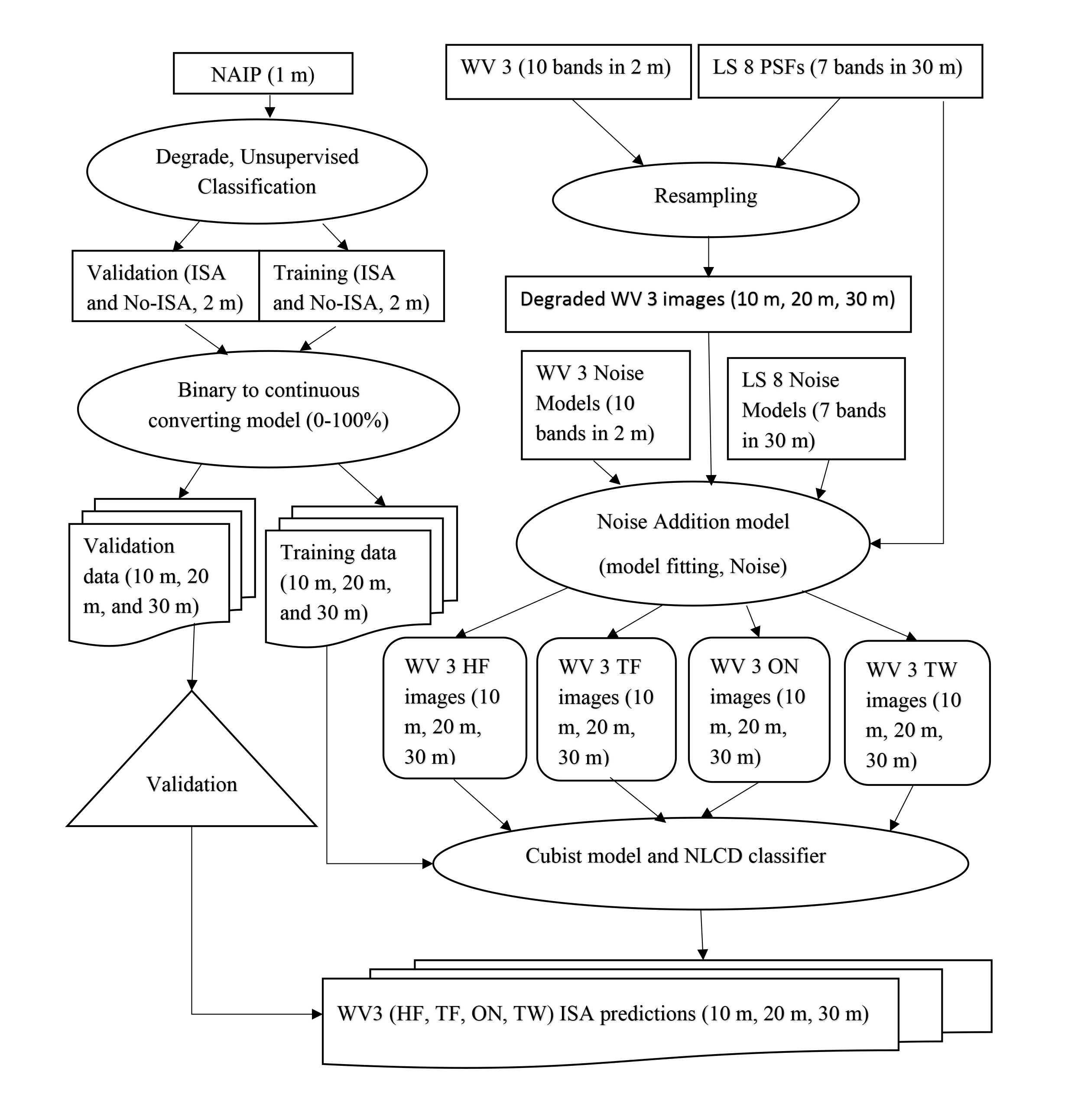
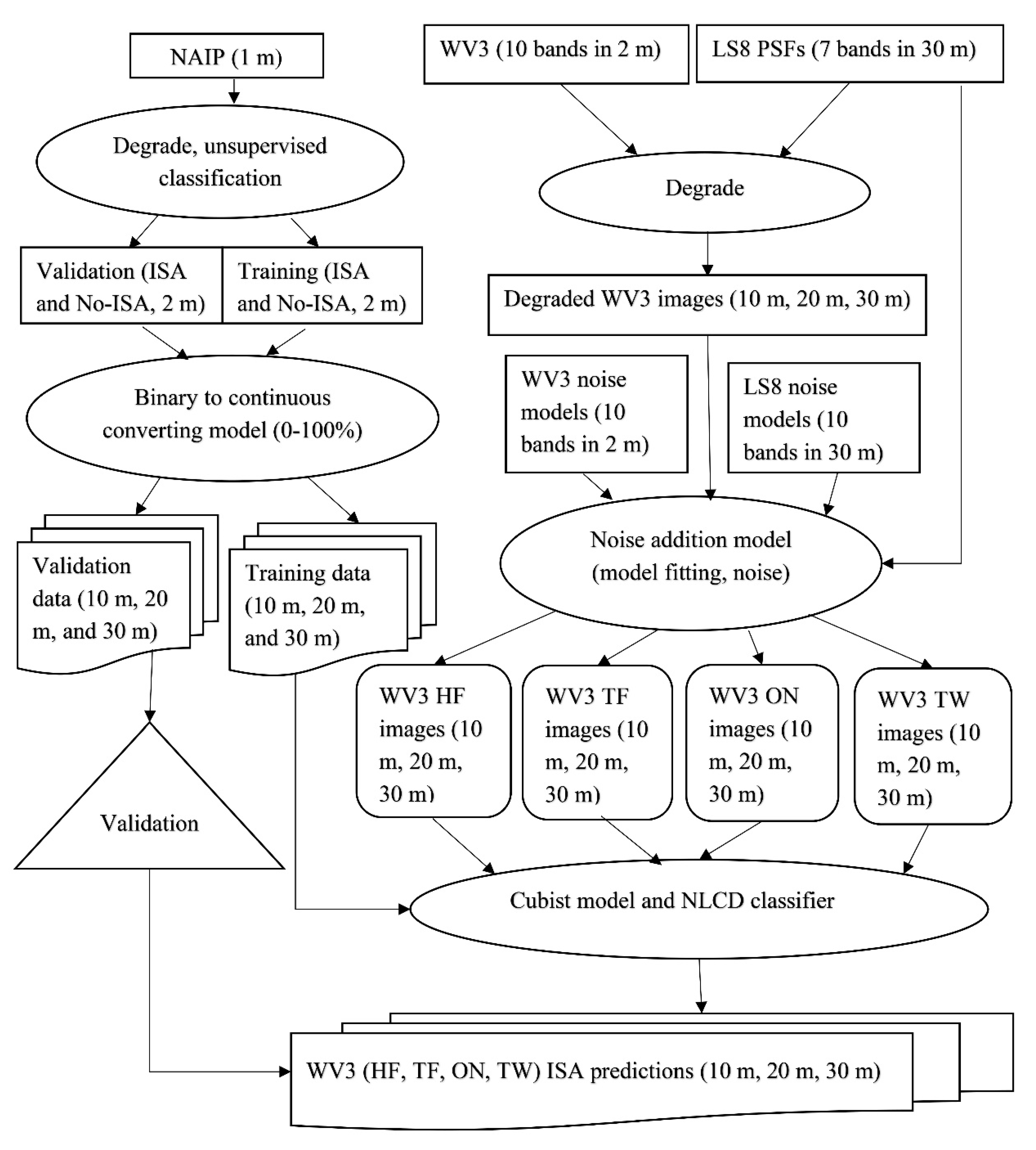
The study was accomplished using several major procedures: selection of study areas; collection of WV3 images; aggregation of WV3 images into three spatial resolutions of 10 m, 20 m, and 30 m; simulation of WV3 images with different SNRs; creation of training and validation datasets; use of regression tree models to estimate ISA; and accuracy assessment. Remote sensing data used in the study included WV3 and National Agriculture Imagery Program (NAIP) images [50], which were used to create high-resolution training and validation datasets for these areas. These training datasets and WV3 images were provided as inputs in the regression models to estimate the percent coverage of the ISA. The overall approach is illustrated in Figure 1.
2.1. Study Area
Two study areas in the United States were selected for this study: Beltsville, Maryland, and San Francisco, California. Beltsville is in northern Prince George’s County, Maryland. The major land cover types in Beltsville are residential housing, roads, commercial/business buildings, and agricultural land. The San Francisco area is the cultural, commercial, and financial center of Northern California. It has very dense tall buildings in the business district. Other urban landscape features include parks, dense road systems, parking lots, bridges, and residential housing. These areas were selected based on the following factors: (1) the diversity of impervious surface features, (2) the presence of mixed pixels that contain imperviousness and other land cover classes, (3) the density of these urban landscapes, and (4) the availability of cloud-free WV3 images.
2.2. Simulation of WV3 Images with Different SNRs
WV3 images, degraded from the original 1.24 m to 2 m resolution, have eight spectral bands from coastal to near-infrared (NIR) (400–1040 nm), eight shortwave infrared (SWIR) bands (1195–2365 nm), and twelve CAVIS (clouds, aerosols, water vapor, ice, and snow) bands (http://worldview3.digitalglobe.com) [51]. Since WV3 images have higher spatial and spectral resolution than the Landsat OLI, it is appropriate to simulate WV3 at different SNR levels and to compare its performance with the Landsat OLI for mapping ISA in the same landscape condition. Due to WV3 data availability and compatibility with the Landsat OLI, WV3 images with only eight spectral bands from coastal to NIR were used for SNR simulations (Table 1). Landsat OLI data was not used in the study.
A remotely sensed image usually contains a substantial portion of the spectral signal of each pixel, not solely from within the footprint of the target pixel, but also from surrounding areas [52]. Many factors including the optics of the instrument, the detector and electronics, and atmospheric effects, as well as image resampling (degraded image spatial resolution), could contribute to this effect [45]. Such effects can be described using the point spread function (PSF), which characterizes a sensor’s response to point signals. In this study, we used the PSF from OLI to resample WV3 images at different spatial resolutions; therefore, the resampled images could have similar spectral features as the OLI. The OLI spatial response for each band is represented in terms of two separable along- and across-track line spread functions [53]. The line spread functions were sampled at four microradian intervals (two microradians for the panchromatic band), providing approximately ten samples per pixel. The separate line spread functions were combined to construct a three-dimensional point spread function for each band. Figure 2 illustrates the two-dimensional subsampled OLI PSFs used for resampling the WV3 images to three different spatial resolutions. The PSFs effectively served as a weighted averaging model for the pixels overlaid by the PSF. The vertices of the PSFs were located at pixel locations in the WV3 imagery. The 30-m PSF had more vertices than the 10-m PSF, so the 30-m PSF overlaid and averaged more pixels.
We used WV3 SNR models provided by DigitalGlobe [54] and reported OLI SNR models [55] to compare the WV3 SNR with the OLI SNR. Subsampling the images with the above PSFs has an averaging effect and improves the SNR on the resulting image by 1 over the root-sum-square of the PSF weights, which ends up being slightly more than for the PSF used (where N is the number of samples overlaid by the PSF). Therefore, the resampled images have better SNRs than the original images. The resampled WV3 images have a higher SNR than the OLI images, so noise must be added to the resampled images to simulate OLI SNR. For this study, three levels of SNR were simulated: ½ OLI SNR (HF), ¾ OLI SNR (TQ), and twice OLI SNR (TW). Noise was added as random Gaussian noise; therefore, noise could be estimated as the standard deviation (σ) of a constant signal. In addition, σ was often used to designate noise models or noise levels. The noise models of the resampled WV3 imagery were random functions, so the additional noise was added in quadrature as defined by Equation (1). The desired noise level was the base resampled (10-m, 20-m, or 30-m) WV3 noise level plus the difference between the base resampled WV3 noise level and the desired HF, TQ, or TW OLI SNR noise level using the standard deviation of the Digital Number (DN), as shown in Equation (2). Substituting Equation (2) into Equation (1) and solving for the amount of additional noise needed produces Equation (3):
where is the noise level of the new, resampled WV3 imagery with the desired fraction of OLI SNR, is the standard deviation of the Gaussian distribution from which the additional noise is selected, is the noise model for the resampled base WV3 imagery, and is the difference between the OLI and resampled WV3 noise models. The amount of additional noise is a random function dependent on the signal level of the imagery, so the amount of noise added to the imagery is different for every pixel and signal level. The different desired noise levels (HF, TQ, and TW) were added on a per pixel basis for each of the resampled images (10 m, 20 m, and 30 m) according to the above equations.
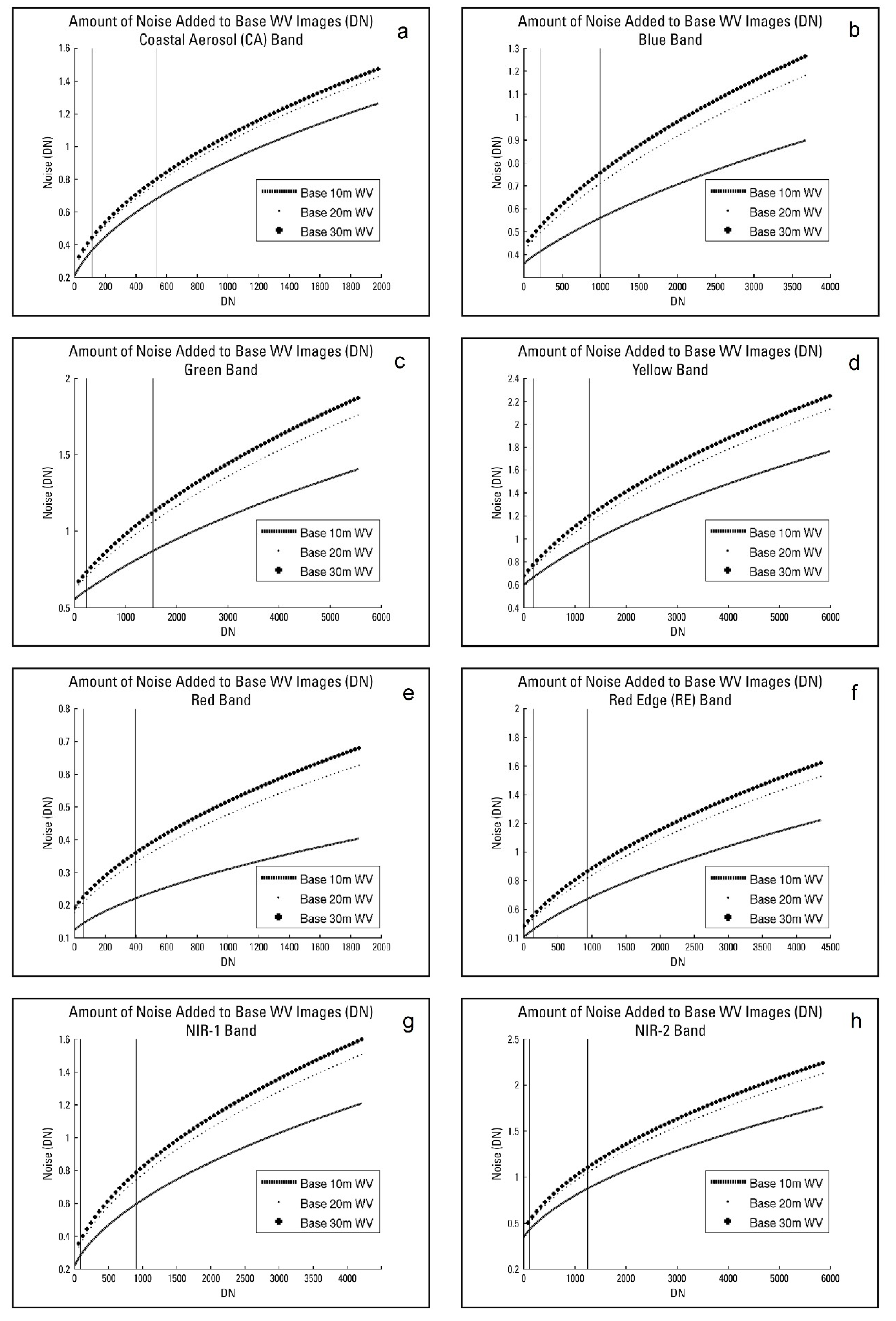
Figure 3 displays the actual noise added in each spectral band to the resampled WV3 imagery to obtain the desired fraction of the OLI SNR that is equivalent to the OLI SNR in this case. For lower SNR levels, more noise was added, and for higher SNR levels, less noise was provided. WV3 imagery has more the visible and near-infrared (VNIR) bands than the Landsat 8 OLI. Therefore, the OLI SNR for the red band was used for the WV3 yellow and red edge bands, and OLI SNR for the NIR band was used for the WV3 NIR1 and NIR2 bands.
3. Impervious Surface Mapping at Different Spatial Resolutions
3.1. Continuous Field Mapping with Remote Sensing Data
Remotely sensed images used in this study included those from NAIP and WV3, as shown in Table 1. To quantify an impervious surface as a continuous field, a regression tree model algorithm, which is a machine learning algorithm and has been widely used to produce the USGS National Land Cover Database (NLCD) continuous field products including impervious surfaces and shrubs/grasses [56,57], is an effective approach [58]. To keep our study results consistent with the NLCD, the same regression tree algorithm was selected for this study. The training and validation datasets were developed first using NAIP images. In each study area, one NAIP image was selected and characterized into impervious and pervious classes using an unsupervised classification approach at a 2-m resolution. The initial unsupervised classification was performed using K-means clustering with 32 classes. These classes were further categorized into different groups and were manually selected as impervious and pervious classes via comparison with the NAIP image. The binary image was further upscaled and converted to 10-m, 20-m, and 30-m resolutions to represent percentages of imperviousness at these scales by using the area-weighted spatial model that was designed using the geospatial data abstraction library (GDAL) and Python to perform the scaling change function [59]. A portion of these fractional ISA data was randomly chosen as training datasets, and other small portions of the data were randomly selected as validation samples. To ensure both training and validation datasets can represent the entire range of imperviousness, both training and validation datasets were sampled across the study area with equal sampling numbers of 1–100%. The locations of sampling points for both training and validation were kept the same when WV3 images with different SNRs were used to map ISA at different spatial resolutions. The numbers of sampling points were reduced from large to small following spatial resolution from fine to coarse. All pixels that were identified as cloud, shadow, water, or no-data, as well as pixels located at the edge of a non-impervious surface, were manually excluded from the training and validation populations. We randomly selected about 97% for training and 3% for validation from the sampled pool of training and validation datasets for both study areas. Table 2 presents the numbers of training and validation samples used in the study. A series of k-fold cross-validations spanned over 10% out of bag and 3% out of bag error estimates (we tested 3–10%). Generally, the 3% out of bag error estimates were consistent with the 10% out of bag error estimates and indicated low overfitting tendencies in the mapping model [58,60]. The training samples were derived from high-resolution images and had limited spatial extension, so the true independent test samples (n = 300) were judiciously (randomly) stratified to capture the data range of the percentage of the impervious surface and to quantify mapping errors between high-resolution training data extents.
The regression tree (RT) modeling algorithms are rule-based predictive models in which a multivariate linear model is associated with a rule or a condition and is created according to the relevant training dataset. A training dataset that contains a dependent variable and several independent variables is required to constrain the parameters in each linear regression equation. The RT models connect the responding variable (dependent variable) to the controlling variables (independent variables) under a specific condition based on their correlations. Generally, a specific WV3 image was used as the controlling variable and the training data was used as the responding variable. Therefore, the frequently used controlling variables or spectral bands of a WV3 image in either conditions or linear equations could be identified in RT models. For this study, WV3 images with different SNRs at 10-m, 20-m, and 30-m resolutions were inputted as controlling datasets.
3.2. Accuracy Assessments for ISA Estimated by Images with Different SNRs
The accuracy assessments for ISA estimated using different WV3 images with different SNRs were performed using validation datasets developed from high-resolution NAIP images. Three statistic metrics were calculated, including root-mean-square-error (RMSE), relative area error (RAE), and mean error (ME) using the following formulas:
where Xobs,i and Xmod,i are a validation measure and a model estimate of percent imperviousness for a sample point i, respectively; Aobs,i and Amod,i are total areas of ISA for a sample point i; n is the number of validation samples; and m is the size of the validation samples within every 1% imperviousness interval. RMSE measures the overall error estimate and RAE estimates the relative difference between the true and model estimated impervious areas. ME measures the mean error in every 1% imperviousness interval so that details about any possible overestimates or underestimates can be revealed. We also evaluated median values between the validation data and ISA estimates from RT models.
4. Results
4.1. Characteristics of Impervious Surfaces from Using Different SNR Data
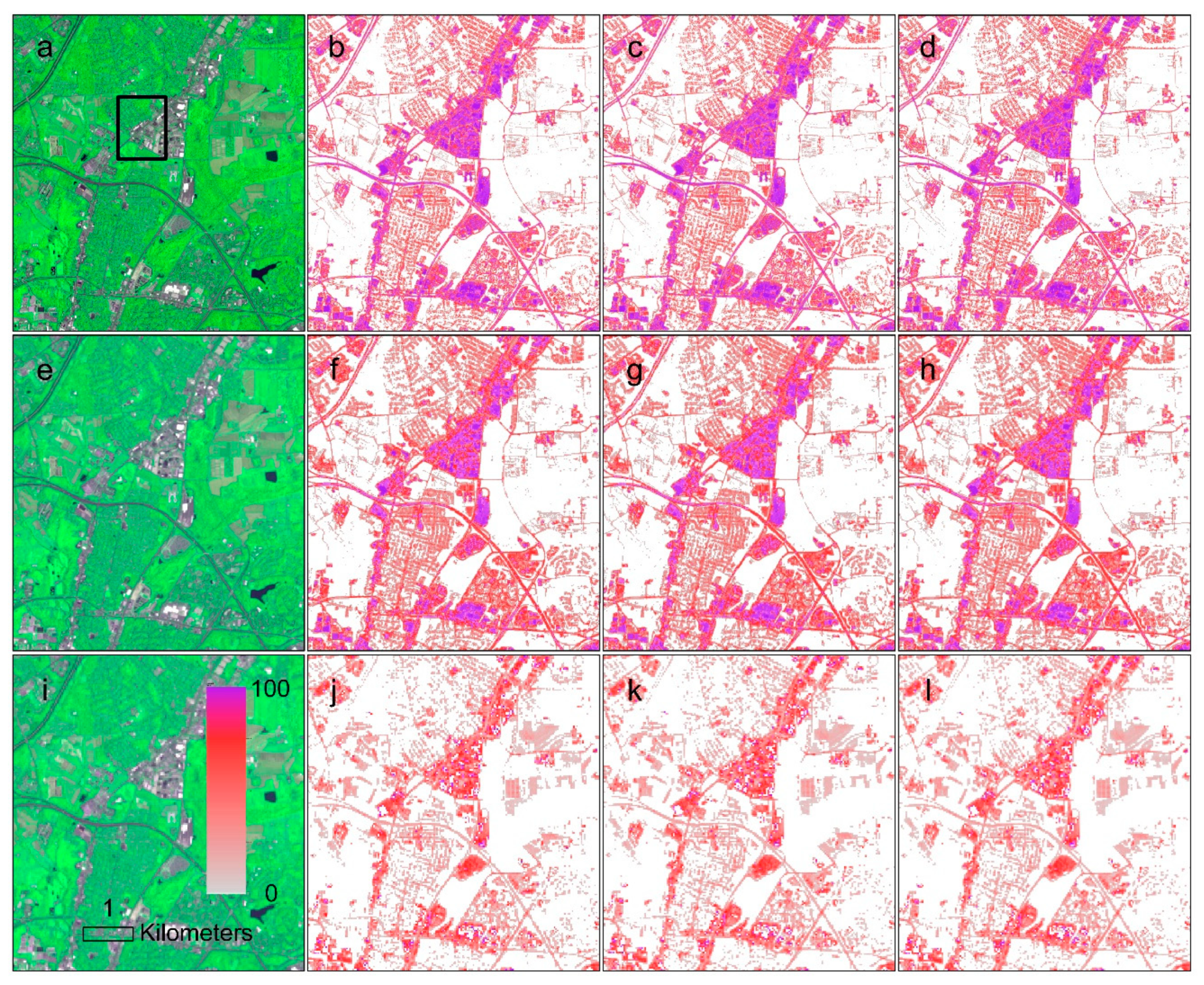
WV3 images and spatial distributions of ISA estimated from RT models using WV3 imagery at 10-m, 20-m, and 30-m resolutions with three different SNRs are presented in Figure 4, Figure 5, Figure 6, Figure 7 and Figure 8 for the two study areas. In the Beltsville area, the estimated ISAs had similar spatial patterns in the same spatial resolution estimate. Specifically, the 10-m estimates (Figure 4b–d) captured more details of the urban landscape and structures with fewer commission errors than the 30-m estimates (Figure 4j–l), regardless of SNR. Furthermore, ISAs estimated from TW images had fewer false estimates in areas with low ISA intensities (Figure 4d,h,l) than other estimates with the same spatial resolution. ISA intensity is defined the same as the percentage of imperviousness. In general, the spatial distributions of the impervious surface estimated from images with the same spatial resolution and different SNRs do not have apparent differences in terms of pattern and intensity. However, WV3 images with high SNRs can capture high-intensity ISAs slightly better and have fewer commission errors in low-intensity ISAs than estimates using images with low SNRs in 10-m and 20-m estimates.
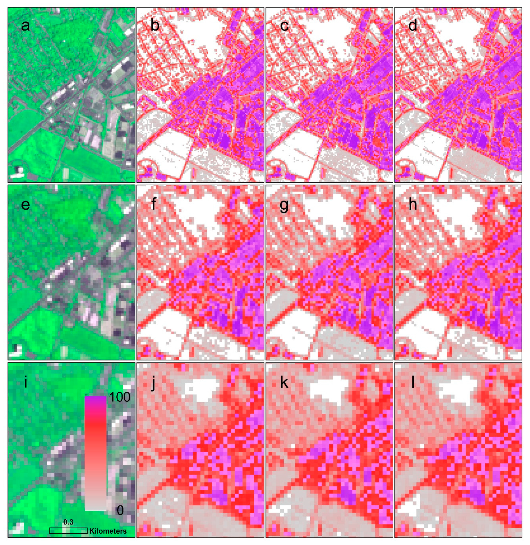
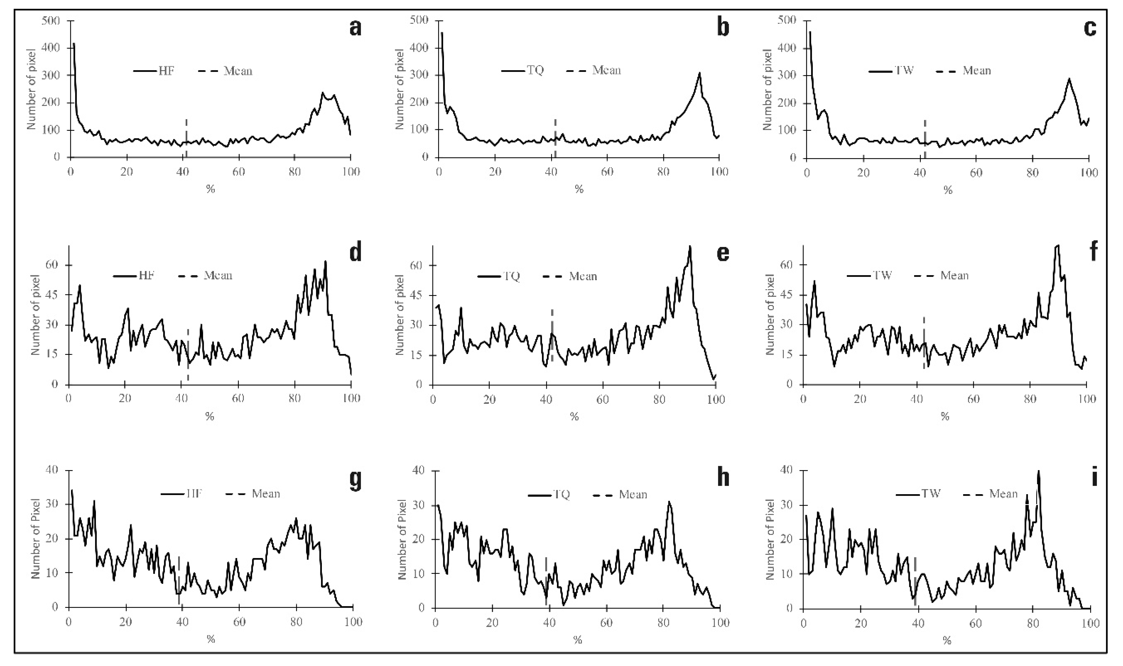
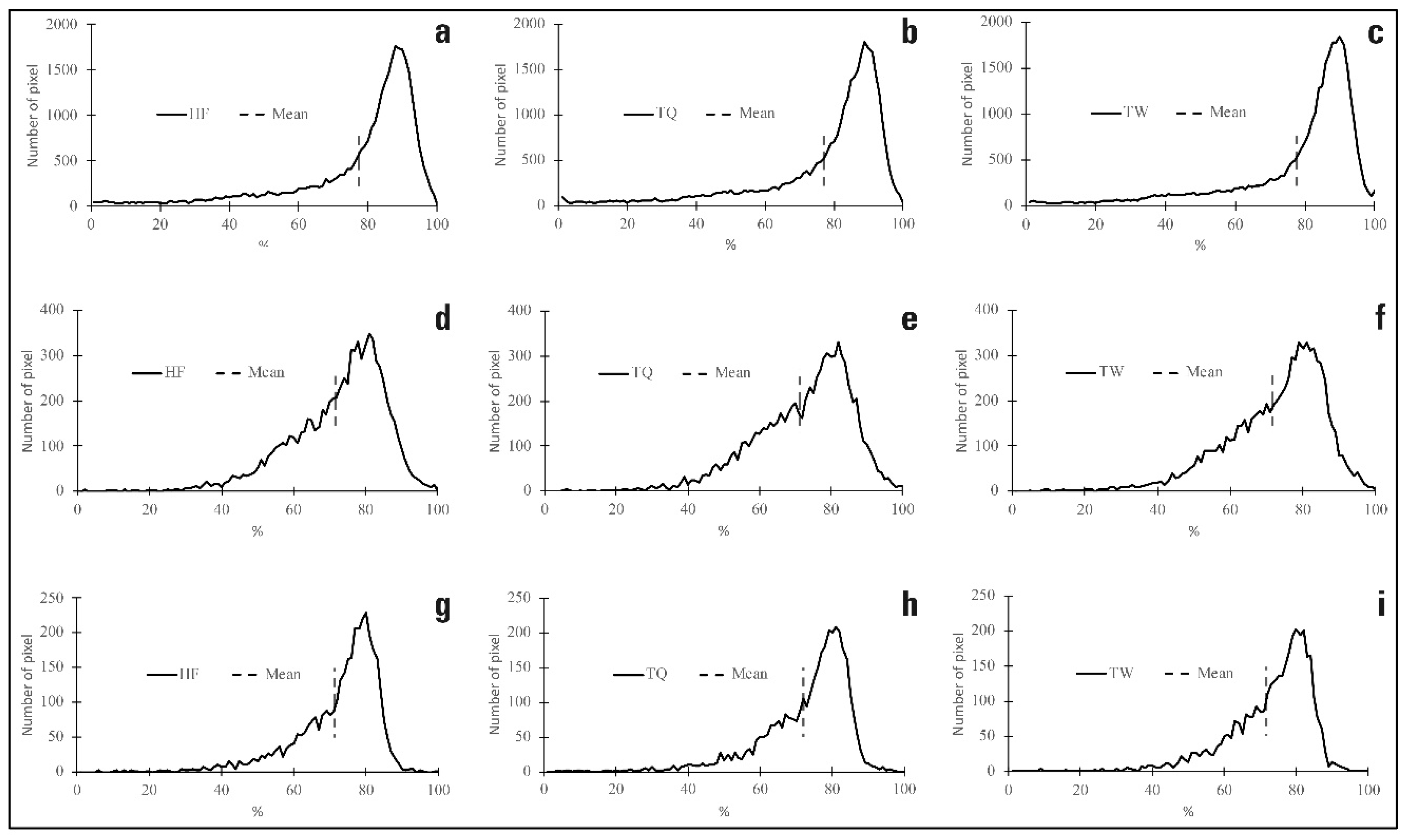
To have a closer look at the ISAs derived from different SNR images, a small zoomed-in area displays WV3 images at different spatial resolutions and derived ISAs (Figure 5). The subset area had a large area of high intensity imperviousness. Details of building structures are captured well in the 10-m estimate. However, there were no apparent differences in ISAs derived from different SNR images at the same spatial resolution. Furthermore, histograms of ISAs from the subset area were also displayed to evaluate their differences in Figure 6. For the 10-m estimate, ISA derived from larger SNR images tended to have relatively more pixels in the high intensity imperviousness area, resulting in the mean in TW moving toward the high ISA (Figure 6a–c). The 20-m estimate had similar distribution patterns of ISA derived from different SNR images (Figure 6d–f). The apparent differences occurred in the 30-m estimate in which the ISAs derived from different SNR images had different histogram patterns without an apparent change in the mean of ISA (Figure 6g–i).
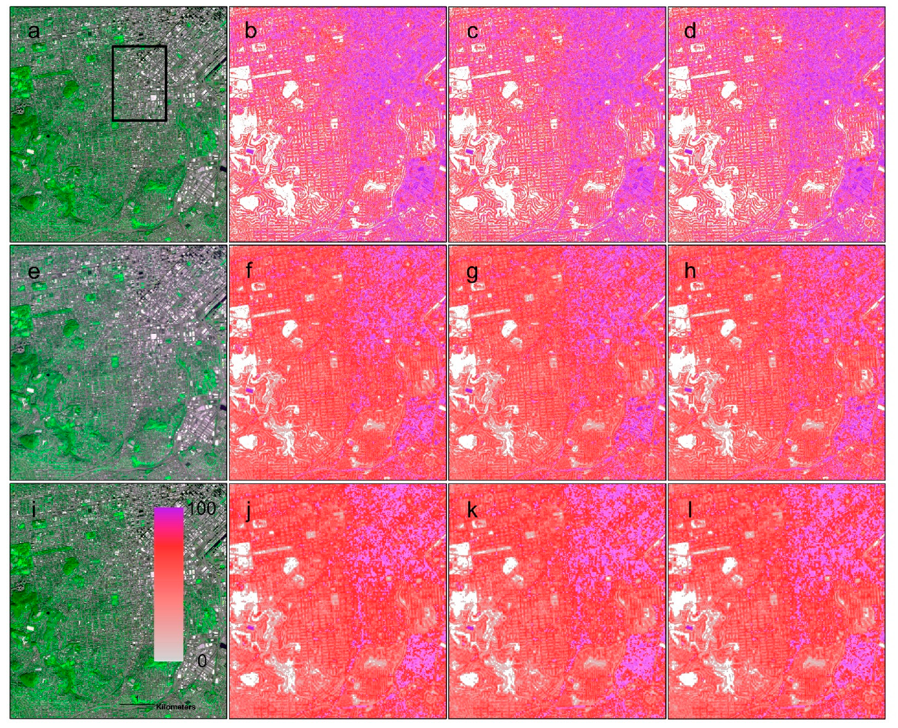
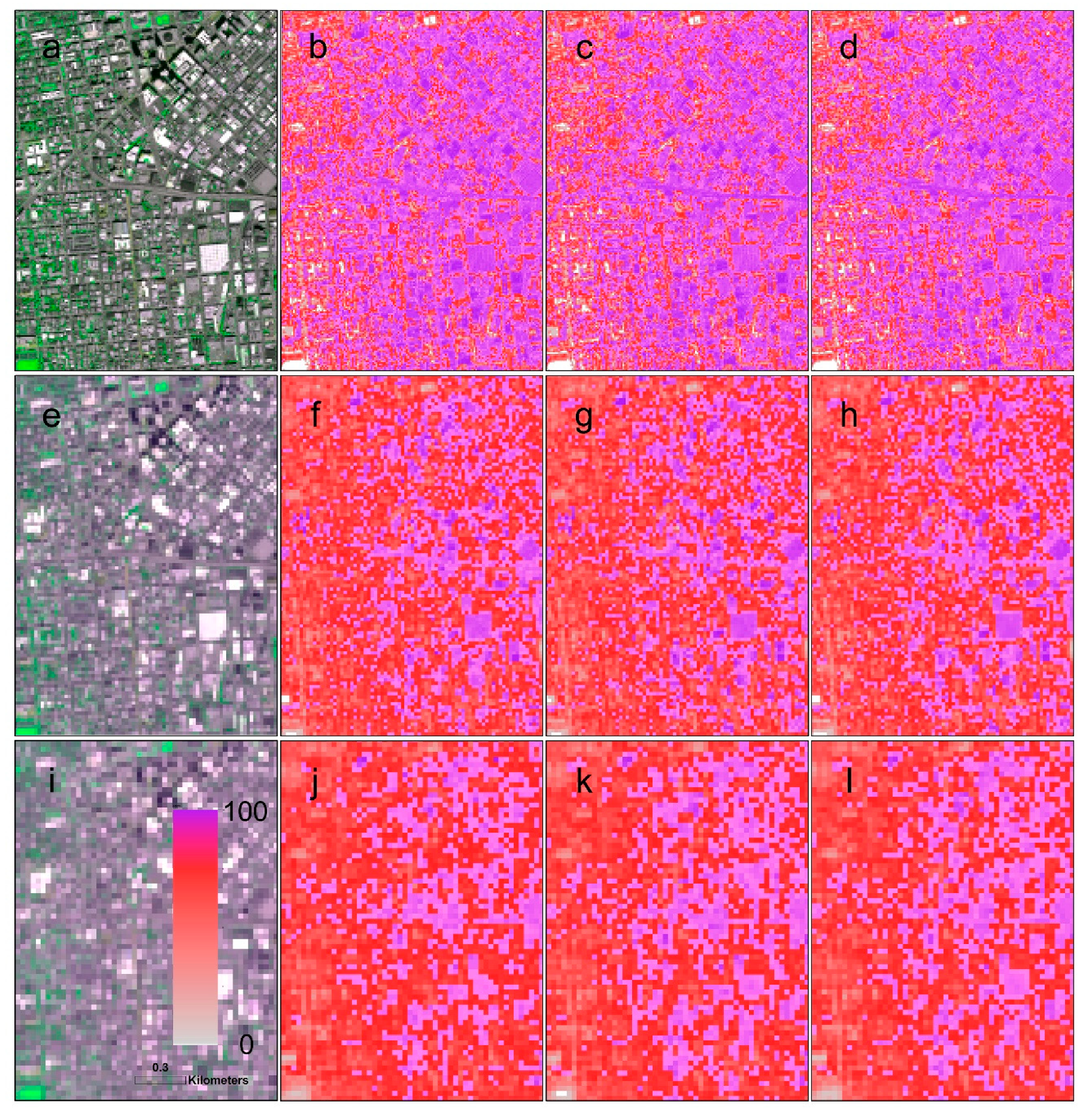
Figure 7—illustrate WV3 images and derived ISAs with different SNRs for the San Francisco area (Figure 7), their distributions in a subset area (Figure 8), and histograms of ISAs from the subset (Figure 9). These figures show consistent distributions of ISAs and their histograms derived from WV3 images with different SNRs, as shown in Figure 3, Figure 4 and Figure 5, in the Beltsville area. The 10-m estimates (Figure 7b–d) captured more details of the urban landscape and structures with fewer commission errors than the 20-m (Figure 7f–h) and 30-m estimates (Figure 7j–l), regardless of the SNR. In the subset area, a large area of high intensity imperviousness associated with high density builds was captured well (Figure 8), especially in the 10-m estimate (Figure 8c–d), without apparent differences in ISAs estimated from different SNR images. However, the 20-m ISA (Figure 8f–h) and 30-m ISA (Figure 8j–l) were apparently different in shape and intensity. Histograms of ISA in the subset area also showed slight differences with different SNRs (Figure 9). For the 10-m estimate, ISAs derived from larger SNR images tended to have slightly more pixels in the high-intensity imperviousness area (Figure 9a–c). Similar distribution patterns of ISAs derived from different SNR images were observed in the 20-m estimate (Figure 9d–f). The apparent differences appeared in the 30-m estimate in which ISAs derived from different SNR images had different histogram patterns (Figure 9g–i).
The RT model outputs listed the first ten most frequently used spectral bands or spectral band derivatives using WV3 images with different SNRs and spatial resolutions in different areas. The model outputs from the two study areas showed that the ranks of spectral bands used in the model had fewer variations with spatial resolution. Also, the use of spectral bands in RT models was not apparently related to the level of the image SNR. In other words, the usage of spectral bands in RT models was more relevant to the landscape conditions.
4.2. Accuracy of Impervious Surface Estimates
We examined several metrics developed from independent validation datasets and modeling estimates to quantify differences in ISA derived from different SNR images. Table 3 and Table 4 illustrate values of RMSE, ME, RAE, square of correlation coefficient (r2), and median values from the validation dataset and model estimates of the percent of imperviousness in Beltsville and in San Francisco.
In Beltsville, the 10-m and 20-m model estimates had similar patterns: RMSE decreased as the SNR increased from HF to TW (Table 3). The ME and RAE had similar patterns in the 10-m estimates but not in the 20-m estimates. In the 20-m estimate, the absolute values of ME and RAE were still the smallest in the estimate from the TW SNR image but were relatively larger in the estimate from the TQ SNR image. In the 30-m estimates, however, the RMSE was the smallest for the HF SNR image, and the absolute values of both ME and RAE were the smallest with the TQ SNR image. Furthermore, for the same SNR, the RMSE value was the smallest in the 20-m estimate and was the largest in the 30-m estimate. The values of ME and RAE did not have such simple patterns. The RMSE values were reduced by about 1.36% and 1.0% in the 10-m and 20-m estimates when the SNR increased from HF to TW. Similarly, the RAE values were also reduced by 1.02% and 0.64% in the same two estimates when the SNR changed from HF to TW. In the 30-m estimate, however, RMSE, ME, and RAE did not have consistent patterns when the SNR increased from HF to TW. The r2 values were the largest in the 20-m estimates. Additionally, r2 values varied slightly for the same spatial resolution with different SNRs. The median values showed that model estimates were closer to validation values by using TW SNR images in all spatial resolutions. By counting all statistic metrics, the estimate of the ISA with the TW SNR image at a 20-m resolution could reach the same level of accuracy with images that had SNRs less than TQ at a 10-m resolution.
In San Francisco, the 10-m and 20-m model estimates had similar variation patterns: both ME and RAE decreased as the SNR increased (Table 4). The RMSE, however, decreased as the SNR increased in the 10-m estimate but not in the 20-m estimate. The RMSE values were reduced by about 4.43% and 0.8% in the 10-m and 20-m estimates when the SNR increased from HF to TW. Similarly, the RAE values were also reduced by 0.44% and 0.27% in the same two estimates when the SNR changed from HF to TW. The r2 values, however, increased slightly as the SNR increased in all resolution estimates. The median values showed that model estimates were closer to the validation values by using TW SNR images in all spatial resolutions. In the 30-m estimate, however, there were no consistent change patterns in RMSE, ME, and RAE when SNR changed from HF to TW. These three metrics were the smallest in the estimate with the HF SNR image.
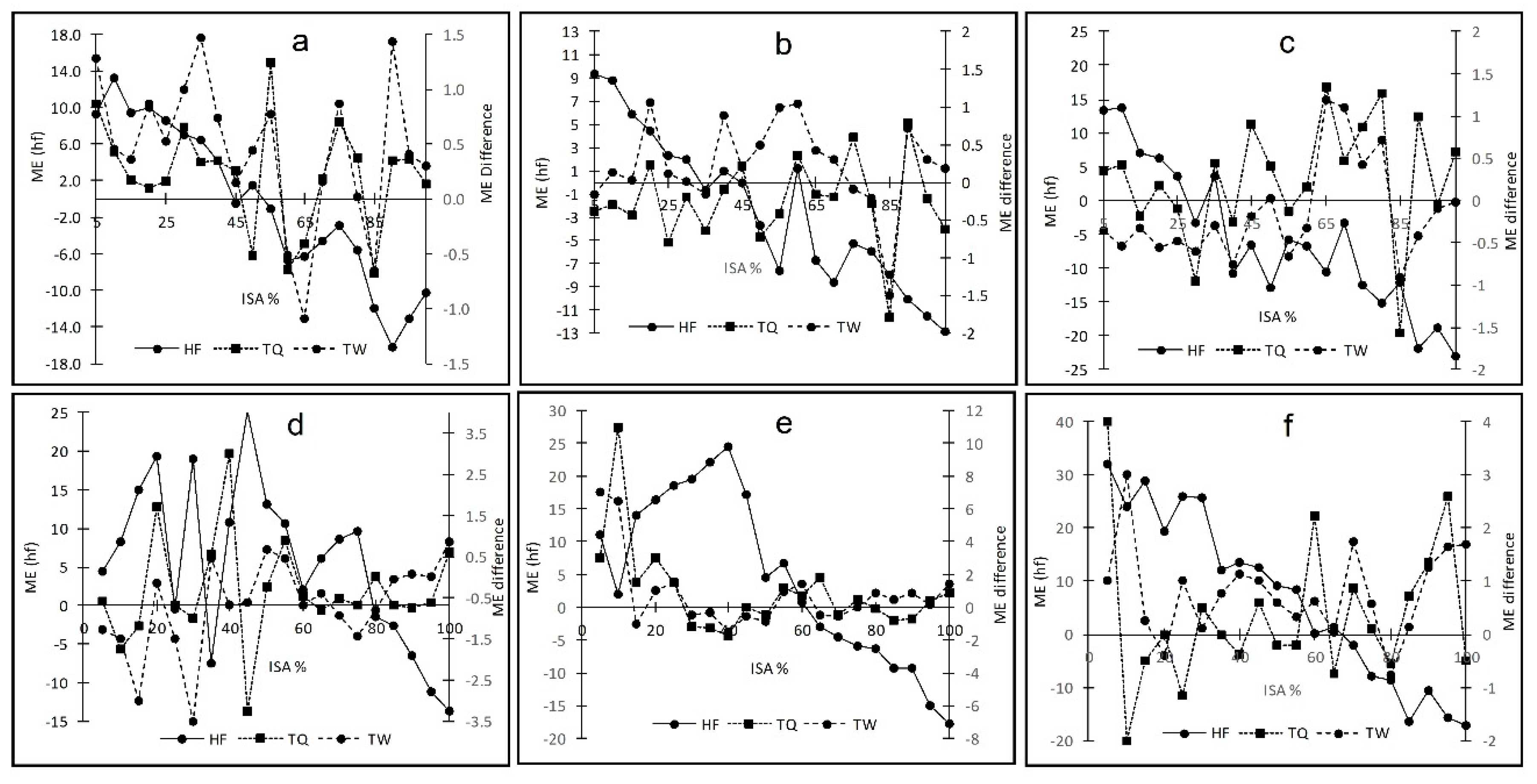
Furthermore, we evaluated the value of ME that was related to the RAE in the ISA estimate. To evaluate the distributions of ME associated with the intensity of the ISA, MEs with every 5% of ISA are displayed for Beltsville (Figure 10a–c) and San Francisco (Figure 10d–f). The MEs from HF are displayed as solid lines and differences of ME between TQ and HF and between TW and HF are shown as dashed lines. In Beltsville, the 10-m estimates (Figure 10a) showed that MEs from three SNR images did not have apparent differences: the ISA was overestimated in ranges below 50% and underestimated in ranges above 50%. The differences of MEs estimated from higher SNR images (TQ and TW) were positive in almost all ISA ranges, and the positive difference was large in the estimate with the TW SNR imagery, resulting in values of ME from negative to slightly above zero. In the 20-m estimates (Figure 10b), the ME from images with HF SNR showed overestimation below 45% and underestimation for most above 45% of ISA. The ME difference between TW and HF SNRs was positive in most ISA ranges, except at 85%. Such an increase in the ME value resulted in the smallest overall ME in the estimate using the image with TW SNR. The negative differences of ME in ranges below 45% of the ISA estimate from the image with TQ SNR indicated ISA underestimation. In the 30-m estimate (Figure 10c), the ME from the image with HF SNR was positive below 30% and negative above 30%. The magnitude of ME from the image with TQ SNR was slightly smaller than the magnitude from the image with HF due to a smaller underestimate in the higher ISA ranges (above 50%). However, the magnitudes from the estimate using the images with TW SNR did not have magnitudes of ME smaller than that derived from the image with HF SNR. The ISAs estimated using the image with TW SNR showed a slightly smaller ME in the ISA intensity less than 40%, as well as around 85%. In general, the overall ME values derived from WV3 images with TW SNR were smaller than those using images with HF SNR in the 10-m and 20-m, but not in 30-m, spatial resolutions.
In the 10-m estimate in San Francisco (Figure 10d), the ME from the image with HF SNR had relatively large positive values in the middle intensity ISA and apparent negative values for ISAs greater than 80%. MEs of the other two estimates from the images with TQ and TW SNRs had slightly positive values for ISAs greater than 60%. These patterns were similar to those in the 10-m estimate in Beltsville. In the 20-m estimates (Figure 10e), the ME from the image with HF SNR showed overestimation between 20% and 45% and underestimation for most above 60% of ISAs. The ME differences between TW and HF, as well as TQ and HF SNRs, were small and positive in most ISA ranges. Such an increase in the ME values from images with TQ and TW SNRs results suggest that ISA estimates could be improved in the middle to high ISA ranges by increasing the SNR. In the 30-m estimate (Figure 10f), the ME from the image with HF SNR was similar to that in Beltsville: positive below 55% and negative above 60%. The differences in ME for TQ-HF and TW-HF were not small. Similar patterns in Beltsville suggest that MEs were not improved upon by increasing SNRs in the 30-m estimate.
5. Discussion
5.1. Impact of Different SNR Data on Impervious Surface Mapping Accuracy
This study evaluated the performance of resolution-reduced WV3 images with different SNRs in estimating a developed impervious surface. Urban landscapes usually have highly heterogeneous features in which developed ISAs are mixed with many other land cover types. The most effective way to characterize these mixing features is to classify urban land cover at the sub-pixel level using the continuous field mapping approach [48,61]. The quality of satellite imagery is critical to accurately quantifying a continuous field in both intensity and areal estimates. In addition to spatial resolution, radiometric performance of remotely sensed imagery could impact the quality of continuous field mapping. The impact of the sensor noise, or SNR, on land cover characterization is not completely understood. The analysis conducted on heterogeneous urban land allowed us to evaluate the dependence of SNR as a function of ISA intensity. In this study, developed impervious surface was used to evaluate the influence of image SNR on the performance of ISA mapping.
The statistical metrics for ISA estimated in the study area suggested that SNR could have a greater impact on 10-m estimates than on 30-m estimates. In general, an increase in SNR from HF to TW could improve the imperviousness areal estimate and reduce error in both 10-m and 20-m estimates, but not in the 30-m estimate.
Mean error is usually used to evaluate an overall error in estimating a continuous variable. However, ME may mislead the overall accuracy assessment when both positive and negative differences between validation and estimated data are added together. To address the uncertainty of overall ME, we also averaged ME values in every 5% bracket of ISAs for different SNR images. In almost all 10-m estimates, the increase of SNR slightly enlarged ME in the lower intensity range of the ISA, where RT models tended to overestimate ISA, as well as in the high intensity range of the ISA, where RT models usually underestimated ISA. This SNR impact pattern was weak in all 20-m estimates and was not notable in most 30-m estimates. The improvement in the high-end of ISA could substantially improve the overall areal estimates. However, overestimates in the lower intensity range could introduce biases in the area covered by more mixed pixels and reduce the detection capability for the low intensity urban area using RT models. Such constraints of the RT model were also found in other studies [54].
The increase of SNR could also intensify some urban signals, resulting in closer to true ISA values than those estimated from HF SNR images at 10-m and 20-m spatial resolutions. However, the 30-m data could contain more mixed land cover types other than urban. Larger SNRs could also enlarge signals from these non-urban areas and therefore produce larger MEs. Such effects are observed in the magnitudes of ME, specifically in medium to low ISAs (Figure 10c,f), RMSE, and RAE (Table 3 and Table 4). Additionally, the MEs generated from images with an SNR higher than HF were less than those from HF images in lower intensity ISA areas. In addition, the PSF model used to resample WV3 images to 30-m resolution averaged more pixels than at the 10-m and 20-m resolutions. Therefore, some surrounding pixels that had non-impervious features could be included in the resampled image. When large SNRs were added to the image, the reduction in noise level for these mixed pixels did not improve the detection of imperviousness.
Furthermore, Figure 5 and Figure 9 represent two types of impervious surface distributions in different geographic locations. Figure 5 represents the area that had mixed vegetation and imperviousness in most pixels. However, Figure 8 displays a high-percentage imperviousness with less vegetation cover.
5.2. Implications for Future Landsat Missions
Landsat satellites have maintained high geometric and radiometric accuracy and have provided science with quality data to support various research and operational applications and are used as the “gold standard” for the calibration of other commercial sensors [62,63]. Looking beyond Landsat 9, the United States Geological Survey (USGS) has collected user needs that emphasize the improvement in spatial, temporal, and spectral resolution in future Landsat data products. However, the SNR required by various applications needs to be evaluated if increased spatial resolution and narrower spectral bands are considered for future Landsat missions. In the case of impervious surface mapping with higher resolution data, a large decrease in SNR could have a stronger impact, and more accurate estimates of ISA could be derived from higher SNR images. However, due to the relatively strong signal from urban features, impervious surface mapping does not require very high SNR levels at a spatial resolution of 30-m. In addition, other applications that require high SNR, such as those relating to coastal or inland aquatic environments, the cryosphere, mapping surface minerals, and studying plant biochemical composition, need particular attention when evaluating sensor characteristics for future Landsat missions.
6. Conclusions
Our study evaluated the impact of the SNR on mapping the developed impervious surface and suggested that the areal estimate could be improved from 1–0.4% and 0.6–0.3% when the SNR changes from half to twice of the Landsat OLI SNR level for simulated WV3 images at 10-m and 20-m resolutions. RMSE could be reduced by 1.4–4.4% and 1.0–0.8% when the SNR had the same change ranges at 10-m and 20-m resolutions. Such improvements were not found when the spatial resolution of simulated WV3 imagery increased to 30-m. The ISA estimates at 10-m had relatively consistent patterns of decreasing RMSE, ME, and RAE with increasing SNR. However, only the RMSEs at the 20-m resolution followed the same trend as at 10-m. Another important improvement with using high SNR imagery in ISA estimates is in areas with high intensity imperviousness. Images with high SNRs can improve the performance of ISA estimates in areas with high intensity imperviousness and can reduce the overall error in areal estimate in 10-m and 20-m estimates. The overall accuracy of ISA at 20-m with a TW SNR image can reach a better than or similar accuracy regarding the ISA at a 10-m resolution with an HF SNR image.
Author Contributions
G.X., H.S., C.A., and Z.W. conceived and designed this study; H.S. collected the data; G.X., H.S., and C.A. analyzed the data; H.S. and G.X. completed the imperviousness mapping, accuracy assessment, and analysis of the results; G.X. led the paper preparation with initial inputs from H.S., and C.A. Z.W. also helped with the initial preparation of the manuscript.
Funding
This research received no external funding.
Acknowledgments
The authors would like to thank the USGS National Land Imaging Program for supporting of this research. We also thank Esad Micijevic, Qiang Zhou, and James Storey for reviewing a draft of the manuscript. Hua Shi’s work was performed under USGS contract G13PC00028.
Conflicts of Interest
The authors declare no conflict of interest. The funding sponsors had no role in the design of the study; in the collection, analyses, or interpretation of data; in the writing of the manuscript, or in the decision to publish the results.
References
- Wulder, M.A.; Coops, N.C.; Roy, D.P.; White, J.C.; Hermosilla, T. Land cover 2.0. Int. J. Remote Sens. 2018, 39, 4254–4284. [Google Scholar] [CrossRef] [Green Version]
- Grekousis, G.; Mountrakis, G.; Kavouras, M. An overview of 21 global and 43 regional land-cover mapping products. Int. J. Remote Sens. 2015, 36, 5309–5335. [Google Scholar] [CrossRef]
- Gong, P.; Wang, J.; Yu, L.; Zhao, Y.; Zhao, Y.; Liang, L.; Niu, Z.; Huang, X.; Fu, H.; Liu, S.; et al. Finer resolution observation and monitoring of global land cover: First mapping results with landsat tm and etm+ data. Int. J. Remote Sens. 2013, 34, 2607–2654. [Google Scholar] [CrossRef]
- Topaloǧlu, R.H.; Sertel, E.; Musaoǧlu, N. Assessment of classification accuracies of sentinel-2 and landsat-8 data for land cover/use mapping. Int. Arch. Photogramm. Remote Sens. Spat. Inf. Sci. 2016, 41, 1055–1059. [Google Scholar] [CrossRef]
- Drusch, M.; Del Bello, U.; Carlier, S.; Colin, O.; Fernandez, V.; Gascon, F.; Hoersch, B.; Isola, C.; Laberinti, P.; Martimort, P.; et al. Sentinel-2: Esa’s optical high-resolution mission for gmes operational services. Remote Sens. Environ. 2012, 120, 25–36. [Google Scholar] [CrossRef]
- Li, X.; Zhou, Y.; Zhu, Z.; Liang, L.; Yu, B.; Cao, W. Mapping annual urban dynamics (1985–2015) using time series of landsat data. Remote Sens. Environ. 2018, 216, 674–683. [Google Scholar] [CrossRef]
- Duro, D.C.; Franklin, S.E.; Dubé, M.G. A comparison of pixel-based and object-based image analysis with selected machine learning algorithms for the classification of agricultural landscapes using spot-5 hrg imagery. Remote Sens. Environ. 2012, 118, 259–272. [Google Scholar] [CrossRef]
- Seto, K.C.; Shepherd, J.M. Global urban land-use trends and climate impacts. Curr. Opin. Environ. Sustain. 2009, 1, 89–95. [Google Scholar] [CrossRef]
- IPCC. The physical science basis. In The Fifth Assessment Report of the Intergovernmental Panel on Climate Change; Cambridge University Press: Cambridge, UK; New York, NY, USA, 2013; p. 36. [Google Scholar]
- Grimm, N.B.; Faeth, S.H.; Golubiewski, N.E.; Redman, C.L.; Wu, J.; Bai, X.; Briggs, J.M. Global change and the ecology of cities. Science 2008, 319, 756–760. [Google Scholar] [CrossRef]
- Weng, Q.; Quattrochi, D.A.; Carlson, T.N. Remote sensing of urban environments: Special issue. Remote Sens. Environ. 2012, 117, 1–2. [Google Scholar] [CrossRef]
- Schneider, A.; Friedl, M.A.; Potere, D. Mapping global urban areas using modis 500-m data: New methods and datasets based on ‘urban ecoregions’. Remote Sens. Environ. 2010, 114, 1733–1746. [Google Scholar] [CrossRef]
- Small, C. A global analysis of urban reflectance. Int. J. Remote Sens. 2005, 26, 661–681. [Google Scholar] [CrossRef]
- Song, X.-P.; Sexton, J.O.; Huang, C.; Channan, S.; Townshend, J.R. Characterizing the magnitude, timing and duration of urban growth from time series of landsat-based estimates of impervious cover. Remote Sens. Environ. 2016, 175, 1–13. [Google Scholar] [CrossRef]
- Sexton, J.O.; Song, X.-P.; Huang, C.; Channan, S.; Baker, M.E.; Townshend, J.R. Urban growth of the Washington, D.C.–baltimore, md metropolitan region from 1984 to 2010 by annual, landsat-based estimates of impervious cover. Remote Sens. Environ. 2013, 129, 42–53. [Google Scholar] [CrossRef]
- Tehrany, M.S.; Pradhan, B.; Jebuv, M.N. A comparative assessment between object and pixel-based classification approaches for land use/land cover mapping using spot 5 imagery. Geocarto Int. 2014, 29, 351–369. [Google Scholar] [CrossRef]
- Shao, Z.; Fu, H.; Fu, P.; Yin, L. Mapping urban impervious surface by fusing optical and sar data at the decision level. Remote Sens. 2016, 8, 845. [Google Scholar] [CrossRef]
- Clark, M.L. Comparison of simulated hyperspectral hyspiri and multispectral landsat 8 and sentinel-2 imagery for multi-seasonal, regional land-cover mapping. Remote Sens. Environ. 2017, 200, 311–325. [Google Scholar] [CrossRef]
- Hansen, M.C.; Loveland, T.R. A review of large area monitoring of land cover change using landsat data. Remote Sens. Environ. 2012, 122, 66–74. [Google Scholar] [CrossRef]
- Gong, P.; Liu, H.; Zhang, M.; Li, C.; Wang, J.; Huang, H.; Clinton, N.; Ji, L.; Li, W.; Bai, Y.; et al. Stable classification with limited sample: Transferring a 30-m resolution sample set collected in 2015 to mapping 10-m resolution global land cover in 2017. Sci. Bull. 2019, 64, 370–373. [Google Scholar] [CrossRef]
- Xian, G.; Crane, M. Assessments of urban growth in the tampa bay watershed using remote sensing data. Remote Sens. Environ. 2005, 97, 203–215. [Google Scholar] [CrossRef]
- Lu, D.; Weng, Q. Use of impervious surface in urban land-use classification. Remote Sens. Environ. 2006, 102, 146–160. [Google Scholar] [CrossRef]
- Sobrino, J.A.; Oltra-Carrió, R.; Sòria, G.; Bianchi, R.; Paganini, M. Impact of spatial resolution and satellite overpass time on evaluation of the surface urban heat island effects. Remote Sens. Environ. 2012, 117, 50–56. [Google Scholar] [CrossRef]
- Mathieu, R.; Freeman, C.; Aryal, J. Mapping private gardens in urban areas using object-oriented techniques and very high-resolution satellite imagery. Landsc. Urban Plan. 2007, 81, 179–192. [Google Scholar] [CrossRef]
- Willkomm, M.; Follmann, A.; Dannenberg, P. Rule-based, hierarchical land use and land cover classification of urban and peri-urban agriculture in data-poor regions with rapideye satellite imagery: A case study of nakuru, kenya. J. Appl. Remote Sens. 2019, 13, 016517. [Google Scholar] [CrossRef]
- Bouziani, M.; Goïta, K.; He, D.C. Automatic change detection of buildings in urban environment from very high spatial resolution images using existing geodatabase and prior knowledge. ISPRS J. Photogramm. Remote Sens. 2010, 65, 143–153. [Google Scholar] [CrossRef]
- Li, P.; Song, B.; Guo, J.; Xiao, X. A multilevel hierarchical image segmentation method for urban impervious surface mapping using very high resolution imagery. IEEE J. Sel. Top. Appl. Earth Obs. Remote Sens. 2011, 4, 103–116. [Google Scholar] [CrossRef]
- Hamedianfar, A.; Shafri, H.Z.M. Detailed intra-urban mapping through transferable obia rule sets using worldview-2 very-high-resolution satellite images. Int. J. Remote Sens. 2015, 36, 3380–3396. [Google Scholar] [CrossRef]
- Pacifici, F.; Chini, M.; Emery, W.J. A neural network approach using multi-scale textural metrics from very high-resolution panchromatic imagery for urban land-use classification. Remote Sens. Environ. 2009, 113, 1276–1292. [Google Scholar] [CrossRef]
- Weng, Q. Remote sensing of impervious surfaces in the urban areas: Requirements, methods, and trends. Remote Sens. Environ. 2012, 117, 34–49. [Google Scholar] [CrossRef]
- Lu, D.; Weng, Q. Extraction of urban impervious surfaces from an ikonos image. Int. J. Remote Sens. 2009, 30, 1297–1311. [Google Scholar] [CrossRef]
- Dare, P.M. Shadow analysis in high-resolution satellite imagery of urban areas. Photogramm. Eng. Remote Sens. 2005, 71, 169–177. [Google Scholar] [CrossRef]
- Hsieh, P.-F.; Lee, L.C.; Chen, N.-Y. Effect of spatial resolution on classification errors of pure and mixed pixels in remote sensing. IEEE Trans. Geosci. Remote Sens. 2001, 39, 2657–2663. [Google Scholar] [CrossRef]
- Lu, D.; Weng, Q. A survey of image classification methods and techniques for improving classification performance. Int. J. Remote Sens. 2007, 28, 823–870. [Google Scholar] [CrossRef]
- Esch, T.; Heldens, W.; Hirner, A.; Keil, M.; Marconcini, M.; Roth, A.; Zeidler, J.; Dech, S.; Strano, E. Breaking new ground in mapping human settlements from space—The global urban footprint. ISPRS J. Photogramm. Remote Sens. 2017, 134, 30–42. [Google Scholar] [CrossRef]
- Zhang, H.; Lin, H.; Wang, Y. A new scheme for urban impervious surface classification from sar images. ISPRS J. Photogramm. Remote Sens. 2018, 139, 103–118. [Google Scholar] [CrossRef]
- Zhang, Y.; Zhang, H.; Lin, H. Improving the impervious surfaces estimation with combined use of optical and sar remote sensing images. Remote Sens. Environ. 2014, 141, 155–167. [Google Scholar] [CrossRef]
- Jensen, J.R.; Cowen, D.C. Remote sensing of urban/suburb an infrastructure and socio-economic attributes. Photogramm. Eng. Remote Sens. 1999, 65, 611–622. [Google Scholar]
- Corner, B.; Narayanan, R.; Reichenbach, S. Noise estimation in remote sensing imagery using data masking. Int. J. Remote Sens. 2003, 4, 689–702. [Google Scholar] [CrossRef]
- Asmat, A.; Atkinson, P.M.; Foody, G.M. Geostatistically estimated image noise is a function of variance in the underlying signal. Int. J. Remote Sens. 2010, 31, 1009–1025. [Google Scholar] [CrossRef]
- De Boer, J.F.; Cense, B.; Park, B.H.; Pierce, M.C.; Tearney, G.J.; Bouna, B.E. Improved signal-to-noise ratio in spectral-domain compared with time-domain optical coherence tomography. Opt. Lett. 2003, 28, 2067–2069. [Google Scholar] [CrossRef]
- Atkinson, P.M.; Sargent, I.M.; Foody, G.M.; Williams, J. Interpreting image-based methods for estimating the signal-to-noise ratio. Int. J. Remote Sens. 2005, 26, 5099–5115. [Google Scholar] [CrossRef]
- Liu, L.; Liu, X.; Hu, J. Effects of spectral resolution and snr on the vegetation solar-induced fluorescence retrieval using fld-based methods at canopy level. Eur. J. Remote Sens. 2017, 48, 743–762. [Google Scholar] [CrossRef]
- Jorge, D.; Barbosa, C.; De Carvalho, L.; Affonso, A.; Lobo, F.; Novo, E. Snr (signal-to-noise ratio) impact on water constituent retrieval from simulated images of optically complex amazon lakes. Remote Sens. 2017, 9, 644. [Google Scholar] [CrossRef]
- Gerace, A.D.; Schott, J.R.; Nevins, R. Increased potential to monitor water quality in the near-shore environment with landsat’s next-generation satellite. J. Appl. Remote Sens. 2013, 7, 1–18. [Google Scholar] [CrossRef]
- Huang, C.; Townshend, J.R.; Liang, S.; Kalluri, S.N.V.; DeFries, R.S. Impact of sensor’s point spread function on land cover characterization: Assessment and deconvolution. Remote Sens. Environ. 2002, 80, 203–212. [Google Scholar] [CrossRef]
- Xie, Y.; Weng, Q. Updating urban extents with nighttime light imagery by using an object-based thresholding method. Remote Sens. Environ. 2016, 187, 1–13. [Google Scholar] [CrossRef]
- Powell, R.; Roberts, D.; Dennison, P.; Hess, L. Sub-pixel mapping of urban land cover using multiple endmember spectral mixture analysis: Manaus, Brazil. Remote Sens. Environ. 2007, 106, 253–267. [Google Scholar] [CrossRef]
- Wu, C.; Murray, A.T. Estimating impervious surface distribution by spectral mixture analysis. Remote Sens. Environ. 2003, 84, 493–505. [Google Scholar] [CrossRef]
- USDA. Naip Imagery. Available online: https://www.fsa.usda.gov/programs-and-services/aerial-photography/imagery-programs/naip-imagery/index (accessed on 1 May 2018).
- Kruse, F.A.; Baugh, W.M.; Perry, S.L. Validation of digitalglobe worldview-3 earth imaging satellite shortwave infrared bands for mineral mapping. J. Appl. Remote Sens. 2015, 9, 096044. [Google Scholar] [CrossRef]
- Forster, B.C.; Best, P. Estimation of spot p-mode point spread function and derviation of a deconvolution filter. ISPRS J. Photogramm. Remote Sens. 1994, 49, 32–42. [Google Scholar] [CrossRef]
- USGS. Landsat Geometry. Available online: https://www.usgs.gov/land-resources/nli/landsat/landsat-geometry (accessed on 1 June 2018).
- DigitalGlobe. Worldview3. Available online: http://worldview3.digitalglobe.com/ (accessed on 1 April 2018).
- Morfitt, R.; Barsi, J.; Levy, R.; Markham, B.; Micijevic, E.; Ong, L.; Scaramuzza, P.; Vanderwerff, K. Landsat-8 operational land imager (oli) radiometric performance on-orbit. Remote Sens. 2015, 7, 2208–2237. [Google Scholar] [CrossRef]
- Xian, G.; Homer, C. Updating the 2001 national land cover database impervious surface products to 2006 using landsat imagery change detection methods. Remote Sens. Environ. 2010, 114, 1676–1686. [Google Scholar] [CrossRef]
- Xian, G.; Homer, C.; Rigge, M.; Shi, H.; Meyer, D. Characterization of shrubland ecosystem components as continuous fields in the northwest united states. Remote Sens. Environ. 2015, 168, 286–300. [Google Scholar] [CrossRef]
- Wylie, B.K.; Pastick, N.J.; Picotte, J.J.; Deering, C.A. Geospatial data mining for digital raster mapping. GISci. Remote Sens. 2019, 56, 406–429. [Google Scholar] [CrossRef]
- Shi, H.; Auch, R.F.; Vogelmann, J.E.; Feng, M.; Rigge, M.; Senay, G.; Verdin, J.P. Case study comparing multiple irrigated land datasets in arizona and colorado, USA. J. Am. Water Resour. Assoc. 2018, 54, 505–526. [Google Scholar] [CrossRef]
- Gu, Y.; Wylie, B.K.; Boyte, S.P.; Picotte, J.; Howard, D.M.; Smith, K.; Nelson, K.J. An optimal sample data usage strategy to minimize overfitting and underfitting effects in regression tree models based on remotely-sensed data. Remote Sens. 2016, 8, 943. [Google Scholar] [CrossRef]
- Maclachlan, A.; Roberts, G.; Biggs, E.; Boruff, B. Subpixel land-cover classification for improved urban area estimates using landsat. Int. J. Remote Sens. 2017, 38, 5763–5792. [Google Scholar] [CrossRef]
- Yang, L.; Xu, R.; Lei, T.; Li, J.; Ouyang, T. Design of near-infrared soil moisture measring instrument. Nongye Gongcheng Xuebao Trans. Chin. Soc. Agric. Eng. 2015, 31, 1–9. [Google Scholar]
- Darwish, W.; Tang, S.; Li, W.; Chen, W. A new calibration method for commercial rgb-d sensors. Sensors 2017, 17, 1204. [Google Scholar] [CrossRef]
Figure 1.
Procedures of mapping and assessing ISAs using WV3 images and Landsat (LS) 8 point spread function (PSF) with different SNRs.
Figure 1.
Procedures of mapping and assessing ISAs using WV3 images and Landsat (LS) 8 point spread function (PSF) with different SNRs.

Figure 2.
Subsampled Landsat OLI point spread function (PSF) for the coastal aerosol band at 10-m (a), 20-m, (b), and 30-m (c) resolutions.
Figure 2.
Subsampled Landsat OLI point spread function (PSF) for the coastal aerosol band at 10-m (a), 20-m, (b), and 30-m (c) resolutions.

Figure 3.
Actual noise added to each WV3 spectral band: coastal (a), blue (b), green (c), yellow (d), red (e), red edge (f), near-infrared 1 (NIR1) (g), and near-infrared 2 (NIR2) (h). The black vertical lines are the defined L-typical radiance for the Landsat OLI, converted to Digital Number (DN).
Figure 3.
Actual noise added to each WV3 spectral band: coastal (a), blue (b), green (c), yellow (d), red (e), red edge (f), near-infrared 1 (NIR1) (g), and near-infrared 2 (NIR2) (h). The black vertical lines are the defined L-typical radiance for the Landsat OLI, converted to Digital Number (DN).

Figure 4.
WV3 images (a: 10 m, e: 20 m, i: 30 m; displayed using bands of R, NIR-1, G), and derived ISAs from images with half, three-quarters, and twice the Landsat OLI SNRs at 10 m (b–d), 20 m (f–h), 30 m (j–l) in Beltsville, Maryland. The non-ISAs are in white.
Figure 4.
WV3 images (a: 10 m, e: 20 m, i: 30 m; displayed using bands of R, NIR-1, G), and derived ISAs from images with half, three-quarters, and twice the Landsat OLI SNRs at 10 m (b–d), 20 m (f–h), 30 m (j–l) in Beltsville, Maryland. The non-ISAs are in white.

Figure 5.
WV3 images at 10-m (a), 20-m (e), and 30-m (i) resolutions from the highlighted area in Figure 4a and derived ISAs from images with half, three-quarters, and twice the Landsat OLI SNRs at 10-m (b–d), 20-m (f–h), 30-m (j–l) resolutions. The non-ISAs are in white.
Figure 5.
WV3 images at 10-m (a), 20-m (e), and 30-m (i) resolutions from the highlighted area in Figure 4a and derived ISAs from images with half, three-quarters, and twice the Landsat OLI SNRs at 10-m (b–d), 20-m (f–h), 30-m (j–l) resolutions. The non-ISAs are in white.

Figure 6.
Histograms of derived ISA from a subset area highlighted in Figure 3. The X-axis is the percentage of ISA and the Y-axis is the total numbers of ISAs derived from images with half (HF), three-quarters (TQ), and twice (TW) the Landsat OLI SNRs at 10-m (a–c), 20-m (d–f), and 30-m (g–i) resolutions. The central vertical dashed lines in each panel represent the mean of the ISAs in each estimate.

Figure 7.
WV3 images (a: 10 m, e: 20 m, i: 30 m; displayed using bands of R, NIR-1, G) and derived ISAs from images with half, three-quarters, and twice the Landsat OLI SNRs at 10-m (b–d), 20-m (f–h), 30-m (j–l) resolutions in San Francisco, California. The non-ISAs are in white.
Figure 7.
WV3 images (a: 10 m, e: 20 m, i: 30 m; displayed using bands of R, NIR-1, G) and derived ISAs from images with half, three-quarters, and twice the Landsat OLI SNRs at 10-m (b–d), 20-m (f–h), 30-m (j–l) resolutions in San Francisco, California. The non-ISAs are in white.

Figure 8.
WV3 images at 10-m (a), 20-m (e), and 30-m (i) resolutions from the highlighted area in Figure 7a and derived ISAs from images with half, three-quarters, and twice the Landsat OLI SNRs at 10-m (b–d), 20-m (f–h), 30-m (j–l) resolutions. The non-ISAs are in white.
Figure 8.
WV3 images at 10-m (a), 20-m (e), and 30-m (i) resolutions from the highlighted area in Figure 7a and derived ISAs from images with half, three-quarters, and twice the Landsat OLI SNRs at 10-m (b–d), 20-m (f–h), 30-m (j–l) resolutions. The non-ISAs are in white.

Figure 9.
Histograms of derived ISAs from a subset area highlighted in Figure 6. The X-axis is percent ISA and the Y-axis is the total number of ISAs derived from images with half (HF), three-quarters (TQ), and twice (TW) the OLI SNRs at 10-m (a–c), 20-m (d–f), and 30-m (g–i) resolutions. The central vertical dashed lines in each panel represent the mean of the ISAs in each estimate.

Figure 10.
Mean error (ME) in impervious surface estimates derived from different SNR images in Beltsville (a–c) and in San Francisco (d–f). ME values were averaged for every 5% of imperviousness. The left y-axis is for ME from images with HF SNR and the right y-axis is for ME differences between estimates from TQ and HF SNR images (TQ-HF: short dashed lines) and from TW and HF SNR images (TW-HF: long dashed lines). The x-axis is the ISA in percent. Panels from the left to the right are the results from 10-m, 20-m, and 30-m estimates.


Table 1.
The source, location, and dates of remotely sensed data used in the study.
| Source (Bands) | NAIP (Blue, Green, Red, NIR-1); WV3 (Coastal, Blue, Green, Yellow, Red, Red edge, NIR-1, NIR-2 (2 m, 10 m, 20 m, 30 m)) | |
| Location | Beltsville, MD | San Francisco, CA |
| Date | 24/07/2015 (NAIP) 17/05/2017 (WV3) | 25/06/2016 (NAIP) 08/03/2017 (WV3) |
Table 2.
Numbers of training and validation datasets.
| Sensor | Area | Beltsville, MD | San Francisco, CA | ||
|---|---|---|---|---|---|
| WorldView-3 | Training | Validation | Training | Validation | |
| 10 m | 10,000 | 350 | 10,000 | 300 | |
| 20 m | 8000 | 290 | 8000 | 250 | |
| 30 m | 7000 | 290 | 7000 | 250 | |
Table 3.
Statistical metrics including RMSE, ME, and RAE in percentages in Beltsville. Correlations between validation data and model estimates, median values in percentage of model estimate (M_m), and validation (M_v).
Table 3.
Statistical metrics including RMSE, ME, and RAE in percentages in Beltsville. Correlations between validation data and model estimates, median values in percentage of model estimate (M_m), and validation (M_v).
| Resolution | SNR levels | RMSE | ME | RAE | r2 | M_m | M_v |
|---|---|---|---|---|---|---|---|
| 10 m | HF | 19.95 | −0.47 | −0.90 | 0.67 | 53 | |
| TQ | 19.83 | −0.22 | −0.42 | 0.67 | 52 | 51 | |
| TW | 19.68 | 0.01 | 0.02 | 0.68 | 51 | ||
| 20 m | HF | 17.29 | −0.34 | −0.82 | 0.70 | 36 | |
| TQ | 17.29 | −0.63 | −1.50 | 0.70 | 36 | 35 | |
| TW | 17.12 | −0.12 | −0.29 | 0.70 | 36 | ||
| 30 m | HF | 22.39 | −1.48 | −3.86 | 0.48 | 30 | |
| TQ | 22.49 | −1.25 | −3.27 | 0.48 | 30 | 31 | |
| TW | 22.43 | −1.71 | −4.47 | 0.48 | 31 |
Table 4.
Statistical metrics including RMSE, ME, and RAE in percentages in San Francisco. Correlations between validation data and model estimates, median values in percentage of model estimate (M_m), and validation (M_v).
Table 4.
Statistical metrics including RMSE, ME, and RAE in percentages in San Francisco. Correlations between validation data and model estimates, median values in percentage of model estimate (M_m), and validation (M_v).
| Resolution | SNR levels | RMSE | ME | RAE | r2 | M_m | M_v |
|---|---|---|---|---|---|---|---|
| 10 m | HF | 17.69 | 0.66 | 1.00 | 0.62 | 76 | |
| TQ | 17.02 | 0.45 | 0.68 | 0.64 | 75 | 71 | |
| TW | 16.90 | 0.37 | 0.56 | 0.65 | 74 | ||
| 20 m | HF | 16.91 | −1.02 | −1.42 | 0.49 | 68 | |
| TQ | 16.94 | −0.79 | −1.21 | 0.49 | 68 | 70 | |
| TW | 16.77 | −0.68 | −1.04 | 0.50 | 69 | ||
| 30 m | HF | 17.28 | 0.95 | 1.54 | 0.46 | 65 | |
| TQ | 17.36 | 1.38 | 2.23 | 0.46 | 65 | 64 | |
| TW | 17.36 | 1.03 | 2.71 | 0.47 | 64 |
© 2019 by the authors. Licensee MDPI, Basel, Switzerland. This article is an open access article distributed under the terms and conditions of the Creative Commons Attribution (CC BY) license (http://creativecommons.org/licenses/by/4.0/).
Share and Cite
MDPI and ACS Style
Xian, G.; Shi, H.; Anderson, C.; Wu, Z. Assessment of the Impacts of Image Signal-to-Noise Ratios in Impervious Surface Mapping. Remote Sens. 2019, 11, 2603. https://0-doi-org.brum.beds.ac.uk/10.3390/rs11222603
AMA Style
Xian G, Shi H, Anderson C, Wu Z. Assessment of the Impacts of Image Signal-to-Noise Ratios in Impervious Surface Mapping. Remote Sensing. 2019; 11(22):2603. https://0-doi-org.brum.beds.ac.uk/10.3390/rs11222603
Chicago/Turabian StyleXian, George, Hua Shi, Cody Anderson, and Zhuoting Wu. 2019. "Assessment of the Impacts of Image Signal-to-Noise Ratios in Impervious Surface Mapping" Remote Sensing 11, no. 22: 2603. https://0-doi-org.brum.beds.ac.uk/10.3390/rs11222603
Note that from the first issue of 2016, this journal uses article numbers instead of page numbers. See further details here.