A Review of Regional and Global Gridded Forest Biomass Datasets


1
Beijing Engineering Research Center of Industrial Spectrum Imaging, School of Automation and Electrical Engineering, University of Science and Technology Beijing, Beijing 100083, China
2
Department of Geographical Sciences, University of Maryland, College Park, MD 20740, USA
3
College of Urban and Environmental Sciences, and Key Laboratory for Earth Surface Processes of the Ministry of Education, Peking University, Beijing 100871, China
*
Author to whom correspondence should be addressed.
Remote Sens. 2019, 11(23), 2744; https://0-doi-org.brum.beds.ac.uk/10.3390/rs11232744
Submission received: 26 October 2019
/
Revised: 15 November 2019
/
Accepted: 19 November 2019
/
Published: 22 November 2019
Abstract
:Forest biomass quantification is essential to the global carbon cycle and climate studies. Many studies have estimated forest biomass from a variety of data sources, and consequently generated some regional and global maps. However, these forest biomass maps are not well known and evaluated. In this paper, we reviewed an extensive list of currently available forest biomass maps. For each map, we briefly introduced the data sources, the algorithms used, and the associated uncertainties. Large-scale biomass datasets were compared across Europe, the conterminous United States, Southeast Asia, tropical Africa and South America. Results showed that these forest biomass datasets were almost entirely inconsistent, particularly in woody savannas and savannas across these regions. The uncertainties in biomass maps could be from a variety of sources including the chosen allometric equations used to calculate field data, the choice and quality of remotely sensed data, as well as the algorithms to map forest biomass or extrapolation techniques, but these uncertainties have not been fully quantified. We suggested the future directions for generating more accurate large-scale forest biomass maps should concentrate on the compilation of field biomass data, novel approaches of forest biomass mapping, and comprehensively addressing the accuracy of generated biomass maps.
1. Introduction
Forests cover about 30 percent of the Earth’s land surface, providing renewable materials and energy for humans, maintaining biodiversity, preventing soil erosion, and playing a major role in the global carbon cycle and climate system [1,2]. As forests grow, they absorb carbon dioxide from the atmosphere via photosynthesis, storing carbon within living biomass and soil, and to a lesser extent, in dead wood and litter. When forests are disturbed (e.g., by fire or deforestation), their stored carbon is released into the atmosphere, therefore an accurate estimation of forest carbon stocks is essential to addressing carbon exchange between terrestrial ecosystems and the atmosphere.
To attain detailed and accurate forest carbon stocks, numerous studies have mapped the spatial distribution of forest biomass using various algorithms assuming that carbon content in plant biomass is constant (approximately 50%). According to the Intergovernmental Panel on Climate Change (IPCC) Guidelines for National Greenhouse Gas Inventories, terrestrial ecosystem carbon pools included above-ground biomass (AGB), below-ground biomass (BGB), necromass and litter. Among these carbon pools, AGB is the most dynamic, visible and important, comprising 15%–30% of the total terrestrial ecosystem carbon pool [3]. Therefore, previous studies on biomass estimation mainly focus on AGB, while BGB is generally determined from AGB using root-to-shoot ratios [4]. In this paper, forest biomass refers to AGB, which is expressed as dry weight per unit area and defined as all living aboveground biomass, including stems, branches, bark, seeds and foliage.
According to dataset sources used to derive forest AGB, estimation methods can be categorized into field measurements, remote sensing-based approaches, and ecological model simulations. Field measurements are valuable resources for biomass estimation as they can provide the most accurate biomass estimates through the use of allometric equations, but are limited in spatial coverage [5,6]. Countries with existing national forest inventory (NFI) data typically use field measurements together with biomass factors and biomass equations to estimate regional means of forest biomass and biomass change for the national forest resources report [7,8]. However, these cannot provide spatially explicit forest biomass information either.
Due to the above limitations of traditional field measurements to estimate biomass on a regional scale, remote sensing has been widely used for estimation during the past decades due to its wide-area coverage capability. In remote sensing-based biomass estimation, field measurements remain important, especially because they are indispensable to both the calibration of remotely sensed data and the validation of estimated biomass results. Importantly, adequate field data is critical to forest biomass mapping from remotely sensed data, no matter which methods are chosen [9]. To estimate forest AGB accurately on a regional scale, much effort is currently being made to integrate field data with remotely sensed data including optical, synthetic aperture radar (SAR) and light detection and ranging (LiDAR) data using advanced methods [10,11,12]. In addition to field measurements and remote-sensing-based methods, ecological process models are promising tools for regional assessment of carbon fluxes and biomass dynamics [13]. However, these models require site specific calibration as well as a large number of input parameters for which appropriate values may be difficult to obtain [14,15]. Therefore, remotely sensed data remain the dominant data sources for AGB mapping. All forest AGB maps selected for inclusion in this paper were retrieved with remotely sensed data in combination with other datasets.
Among the three types of remotely sensed datasets, LiDAR is recognized as the most accurate and promising approach for AGB estimation, but cannot provide wall-to-wall biomass results [16]. In contrast, optical and SAR data can provide gridded AGB estimates over large areas, but are affected by well-known saturation problems that greatly affect the accuracy of estimated biomass. No single sensor on any satellite mission, whether optical, radar or LiDAR, can provide consistently infallible estimates of biomass, so a combination of these measurements is often used to overcome individual limitations [17]. Therefore, many scholars have integrated field measurements, LiDAR, optical and/or SAR data using advanced methods to generate maps of the spatial distribution of forest AGB on a regional scale [18,19]. Currently, many regional and global AGB maps are available, and some of them have been even used for further analysis in the fields of climate change and ecology [20,21,22,23]. However, published papers mainly review biomass estimation methodologies, focusing on the datasets used, modelling algorithms, uncertainties and other related issues [9,24,25,26], and a systematic review of forest AGB maps is still lacking. While in this paper, we collected currently available regional and global forest biomass maps, and described their retrieval and limitations, to address recent progress and practical challenges of large-area biomass mapping. Forest biomass estimation or mapping is a complex procedure involving many factors, so we focused only on the major aspects of estimating forest AGB.
The paper is organized as follows: Section 2 introduces the principles for using remote-sensing-derived parameters for AGB estimation; Section 3 describes the currently available regional and global forest biomass maps; Section 4 compares the available forest biomass maps over several regions; Section 5 includes the limitations of current forest AGB maps and possible directions to improve their accuracy; and Section 6 is a brief summary.
2. Principles for Estimating AGB from Remotely Sensed Data
Generally, remote sensing techniques do not derive forest biomass directly, but use parameters that are related to forest biomass such as forest height, leaf area index, or net primary production. Because of established relationships with AGB, these parameters or variables are widely incorporated into the mapping of forest AGB.
Forest height is often used as a surrogate for biomass. At the plot scale, AGB estimates are usually made using allometric equations that are based on hand-measured tree diameters and/or tree height, sometimes with wood density to improve accuracy [27]. The relationship between AGB and tree height generally follows a power law function. Published studies have indicated that the close relationship between forest biomass and height developed at the tree and plot scale still hold at a broad scale [28]. Since height can be directly obtained from Interferometry SAR (InSAR) and LiDAR data over large areas [29,30], forest AGB can be estimated from these remotely sensed data. It should be noted that height sometimes refers to canopy height (e.g., InSAR height), which depends not only on tree height, but also on the shape of each tree crown and on stand density. Some studies indicate that tree crown or basal area might be a better indicator of biomass than tree height, and thus basal area weighted height (or Lorey’s height) was proposed as the best proxy for biomass and widely used in LiDAR remote sensing [12,19,31].
Previous studies have found LAI is also a valuable AGB predictor, and have developed methodologies to estimate AGB from LAI [32]. LAI is mainly related to leaf biomass, and therefore foliage or leaf biomass can be quantified through a function of LAI and specific leaf area (SLA) which is the ratio of leaf surface area to carbon mass [33]. At the plot scale, total AGB is generally computed as the sum of wood and foliage biomass [34], but at larger scales, there have been two general approaches to establish a relationship between LAI and forest biomass. One estimates the components of AGB separately, which follow similar equations and can be derived in the same way as foliage biomass, and then calculates the sum of these biomass components. The other approach is to develop relationships between foliage biomass (or LAI) and AGB directly, in terms of the allocation of forest biomass carbon into different parts including leaves. Using either method, the proportion of foliage biomass in AGB varies with forest type, stand age, and environmental factors [35].
Similar to that of LAI, the relationship between tree productivity and biomass has been explored in previous studies that often use the demonstrated relationship to estimate AGB directly, either linear or nonlinear, assuming that productivity is the source of biomass [36]. Another approach to estimate AGB comes from the metabolic theory of ecology which describes the rates of production and biomass by a power function [37]. Also, the relationship between AGB and productivity varies with certain biotic and abiotic factors [38].
As a measure of chlorophyll abundance and energy absorption, the normalized difference vegetation index (NDVI) has been widely used as a proxy for vegetation productivity and foliage biomass [39,40]. It is sensitive to the green components of biomass but insensitive to woody components where the majority of forest carbon is stored. One limitation of applying NDVI to estimate biomass is the saturation effect due to strong absorption in the red wavelength. With an increase in green vegetation, the sensitivity of NDVI and furthermore, the accuracy of estimated biomass is reduced. To improve sensitivity across the regions with high biomass, several vegetation indices were proposed such as the renormalized difference vegetation index and the modified simple ratio [41,42]. Moreover, the vegetation optical depth (VOD), derived from satellite passive microwave observations, is mainly sensitive to the water content and captures variations in foliage biomass better than NDVI in drylands, and thus can provide complementary information for estimating green biomass in dryland areas [39,43].
Forest cover is another important AGB predictor, especially where forest cover is less than 60%. For uniform forests, forest biomass of a pixel is directly proportional to forest cover [44]. Currently, several forest cover products are available on a global scale, facilitating the estimation of forest biomass [45]. However, the proportional tree or forest cover could reach its maximum before forest biomass, which limits the performances of biomass estimation to some degree.
Further to the above ecological process parameters, topographic and biotic factors (e.g., species diversity) are known to affect forest biomass. From the data perspective, the relationships between the abovementioned parameters and AGB vary with topographic and biotic factors. Topographic characteristics such as elevation and aspect are known to drive patterns of tree species distribution, as well as soil resources, both of which influence AGB. From another perspective, these factors regulate carbon storage in forest ecosystems [46]. Finally, since AGB in a forest integrates establishment, growth and mortality processes, as well as succession, disturbance, and ecosystem processes, the inclusion of these data could improve the accuracy of AGB estimates [47,48].
3. Current Gridded Forest Biomass Maps
Current gridded forest biomass maps are generated mainly through empirical modeling of various datasets (Table 1). We grouped these regional and global AGB maps into the following five classes according to the combinations of data sources used in the estimation. Forest biomass maps of the first class were mainly obtained through Geographic Information System (GIS) based modelling of statistical datasets. Sixteen AGB maps were generated by integrating field biomass data directly with optical and/or radar data. Five datasets were retrieved from field biomass data together with LiDAR data, and thus had high spatial resolution. Fourteen AGB maps were generated from a combination of field data, LiDAR data, and optical and/or radar data. Also, there were some AGB maps that were generated or regenerated from existing biomass datasets.
3.1. Forest AGB Maps Generated Using GIS-Based Methods
3.1.1. New IPCC Tier-1 Global Biomass Carbon Map for the Year 2000
Ruesch and Gibbs [49] compiled a total of 124 carbon zones or regions with unique carbon stock values using the IPCC (International Panel on Climate Change) Tier-1 method [50]. Then, they incorporated these values with spatial datasets including land cover maps, ecoregions zones, continental regions, and frontier forest location maps, to generate a global biomass carbon map with a spatial resolution of 1 km. This dataset is the first globally consistent and spatially explicit estimate of vegetation biomass and carbon stocks, circa 2000. It has important implications for climate and environmental change studies, however, the methods employed in the generation of the dataset were not directly related to field measurements or validated with field data, and little is known about uncertainties in the map.
3.1.2. A Map of Living Forest Biomass and Carbon Stock in Europe
Using a similar approach to Ruesch and Gibbs [49], Barredo et al. [51] provided a forest biomass dataset for Europe at 1 km spatial resolution for the year 2010. They first estimated forest biomass from the CORINE Land Cover 2006 map, then the average biomass value of each ecological region from the Food and Agriculture Organization (FAO) Global Ecological Zone (GEZ) map, and then post-adjusted the estimates at pixel level for each country by applying adjustment ratios to match the national values reported in the FRA 2010 [52]. The generated map corresponded with biomass and carbon reported in FRA at the country level and therefore at a continental level. However, due to a lack of field data, the map was not validated at the pixel level.
3.1.3. Global One-Degree Maps of Forest Area, Carbon Stocks, and Biomass, 1950–2010
Based on a compilation of forest area and growing stock data reported in international assessments performed by the FAO, MCPFE (now Forest Europe) and the United Nations Economic Commission for Europe, Hengeveld et al. [53] provide global forest biomass at 1° spatial resolution with five-year intervals from 1950 to 2010. They initially used a ratio between forest area (from a forest raster map) and the interpolated forest area value (calculated from the international assessments performed by FAO, MCPFE, and UNECE) to scale the raster values in the forest map. Then, the growing stock gridded map was derived from interpolated forest growing stock data divided by the adjusted forest area, and multiplied with calculated forest area maps. Finally, forest growing stock were converted to biomass and carbon using the IPCC default biomass conversion and expansion factors [50]. Uncertainty in this dataset was subjectively defined as the sum of basic data uncertainty, methodological developments over time, and interpolation and mismatch between the forest map and statistical data, but it was not formally evaluated.
3.1.4. IIASA’s Global Forest Database
Kindermann et al. [54] produced a global forest biomass database at 0.5° resolution for the year 2005 by downscaling the aggregated country-level FRA biomass, on the basis of the relationships between net primary productivity (NPP) and biomass, and between human impact and biomass. The uncertainty of estimated AGB depends heavily on the quality of the FRA, and NPP and human activity data, as well as the simple assumption of linearity in the relationship between NPP and human activity, and biomass.
3.1.5. Tropical Africa and Southeast Asia 1980 and 2000 Forest Biomass Maps
The above maps were derived as a function of degradation ratio (DR) and potential biomass density obtained from climate, soil, topographic, and land-use information using rule-based GIS models [55,56,57,58]. Potential biomass was calculated based on land cover data, while the DR was closely correlated with population density. Forest biomass maps for 2000 with a spatial resolution of 0.045 decimal degrees produced by Gibbs and Brown [57,58] were updated from those for 1980, by including land cover data from GLC2000 and population data in 2000. For both the 1980 and 2000 biomass datasets, the same equations were used to calculate DR, which was estimated by comparing the potential biomass density in 1980 with the corresponding biomass densities obtained from forest inventories. The parameters varied for different forests (open or closed, woodland or savanna), but followed the same patterns.
where PD is a population density in people per km2. Different forest types had different parameter values of a and b, but they were the same for 1980 and 2000 for the same forest type. Because PD in 1980 and 2000 was different, their corresponding DRs were different. Uncertainties of both biomass datasets were not reported, and additional field data are needed to assess the accuracy of this dataset.
DR = a − b ln(PD)
3.2. Forest AGB Maps from Field Inventory Data and Optical and/or Radar Remotely Sensed Data
3.2.1. National Biomass and Carbon Dataset for the Year 2000
The Woods Hole Research Center generated a high-resolution (30 m) “National Biomass and Carbon Dataset for the Year 2000” (referred to as NBCD) for the conterminous United States [59]. The dataset was based on an empirical modelling approach that combined FIA data with optical remote sensing data acquired from the Landsat ETM+ sensor, high-resolution InSAR data acquired from the Shuttle Radar Topography Mission (SRTM), products from the USGS NLCD 2001 (National Land Cover Dataset 2001, land cover and canopy density) and LANDFIRE (the Landscape Fire and Resource Management Planning Tools Project, existing vegetation type) projects, and topographic information from the USGS National Elevation Dataset (NED). The NBCD provided two biomass maps based on different allometric equations to calculate tree-level biomass. The version of the NBCD map based on FIADB Tree Table to calculate tree biomass, which was also the source of the 240 m mosaic for the conterminous U.S, has often been adopted in published studies. NBCD provided the accuracy for each mapping ecoregion through validation against observed data from USDA Forest Service Forest Inventory and Analysis (FIA). Because of the good verification accuracy with FIA data, NBCD2000 is often used in forest research, however, it significantly overestimated biomass in urban areas [60,61].
3.2.2. Forest Biomass across the Lower 48 States and Alaska
Blackard et al. [44] produced a forest AGB map at a spatial resolution of 250 m for the conterminous United States, Alaska, and Puerto Rico by interpolating the FIA plot data collected from 1990 to 2003 with geospatial predictors using the classification and regression tree modelling approach. The predictors included the Moderate Resolution Imaging Spectroradiometer (MODIS) data acquired during 2001, land cover proportions, topographic variables, monthly and annual climate information, and other ancillary variables. The accuracy of the AGB map was reported as correlation coefficients ranging from a low of 0.31 in the southern region of the United States to a high of 0.92 in Puerto Rico, and relative errors ranged from 0.92 in the southern region of the United States down to 0.51 in Puerto Rico. Due to the saturation phenomenon caused by optical remote sensing data and the problem of scale conversion between the FIA data and pixel scale, the low biomass density of this datasets was overestimated, and high biomass density was underestimated [62]. AGB uncertainty was assessed by the relative error of modelled predictions and an error propagation approach, which allowed for the incorporation of pixel-level uncertainties when other sources were lacking.
3.2.3. Forest Carbon Stocks of the Contiguous United States (2000–2009)
Wilson et al. [63] mapped the contiguous United States forest carbon stocks between 2000 and 2009 at a 250 m resolution from FIA data, MODIS satellite imagery, and ancillary geospatial datasets using the Phenological Gradient Nearest Neighbor approach. The published datasets also contained total carbon stocks, live tree aboveground forest carbon, live tree belowground forest carbon, down dead wood carbon, forest litter carbon, forest standing dead carbon, forest soil organic carbon, and forest understory carbon. Uncertainty maps were not provided with the carbon maps.
3.2.4. Aboveground Biomass in Interior Alaska (Yukon River Basin), 30 m, 2009–2010
Ji et al. [64] combined a field biomass dataset with Landsat-derived spectral variables and land surface temperature (LST) using a regression model, and produced a biomass map at 30 m resolution for the Yukon Flats ecoregion of interior Alaska. The geographic feature metrics included land cover type sourced from the NLCD 2001, burned areas from the Monitoring Trends in Burn Severity (MTBS) data and the Alaska Historical Wildland Fire Perimeters data, and topographic futures extracted from National Elevation Dataset (NED) data. Additionally, before building the regression model, principal component analysis (PCA) was used to prevent variable multicollinearity. A high-spatial resolution biomass map was generated using the principal components and field data through a regression method. This map appears relatively accurate as evidenced by a threefold cross-validation that showed a mean absolute error of 21.8 Mg/ha and a mean bias error of only 5.2 Mg/ha.
3.2.5. The First Detailed Map of Aboveground Forest Carbon Stocks in Mexico (30 m)
Cartus et al. [65] generated a spatially explicit map of aboveground carbon stored in Mexico’s forests at 30 m spatial resolution through Random Forest modelling on the inventory data from Mexico’s National Forest Inventory (INFyS) and space borne optical and radar data including the Advanced Land Observing Satellite (ALOS) Phased Array type L-band Synthetic Aperture Radar (PALSAR) backscatter data, Landsat-based estimates of canopy density, MODIS vegetation index product, and topographic data from SRTM. Validation results with independent field data showed that the overall R2 was 0.5 and the root mean square error (RMSE) was 14 t C/ha in flat areas, with low predicted precision on steep slopes.
3.2.6. Mexico Forest Biomass Map (250 m)
Rodríguez-Veiga et al. [66] generated a forest biomass map for Mexico at 250 m spatial resolution by combining remotely sensed predictors with forest inventory plots using a maximum entropy (MaxEnt) algorithm. The predictors were extracted from MODIS vegetation index products, ALOS PALSAR backscatter coefficient images, and the SRTM digital elevation model. The generated forest biomass map was validated with independent inventory plot data at the 50 m pixel level, municipality level, and state level. The validation results showed that the accuracy was improved along with the spatial scale from pixel level to municipality and state level, with the RMSE of 17.3 t C/ha, ±4.4 t C/ha, and ±2.1 t C/ha, and R2 of 0.31, 0.75 and 0.94, respectively. At the pixel level, map uncertainty was quantified through an error propagation model which accounted for measurement, allometry, sampling, and remote sensing prediction errors, assuming that these source errors were random and independent. Although this study provided accurate spatial maps for national or regional REDD+ applications and MRV systems, uncertainties still cannot fully meet the requirements anticipated for the planned BIOMASS mission [67].
3.2.7. Maps of Canada’s Forest Attributes for 2001 and 2011
Beaudoin et al. [68] produced forest biomass maps for Canada at 250 m resolution for 2001 using k-nearest neighbours (kNN) method. The predictors included MODIS reflectance data, climatic variables, topographic variables and land cover information. Validation of estimated forest biomass with the independent field data at the pixel level showed that the R2 was 0.69 and the relative RMSE was 69.2%, but that accuracy could be improved if the pixels were spatially aggregated to 1 km resolution. A biomass map for 2011 was similarly generated. To infer biomass dynamics from the sequential biomass maps, Beaudoin et al. [69] updated the 2001 and 2011 forest biomass estimates [68]. The new forest biomass datasets were generated using an improved reference dataset sourced from Canada’s National Forest Inventory (NFI) and a refined kNN method. Evaluation results were in better agreement than that of Beaudoin, Bernier, Guindon, Villemaire, Guo, Stinson, Bergeron, Magnussen and Hall [68], and showed that changes in aboveground biomass matched expectations between 2001 and 2011 where fire, harvest, or post-disturbance regrowth occurred.
3.2.8. EU-Wide Growing Stock and Biomass Maps
Gallaun et al. [70] linked field inventory plot data directly to remotely sensed data using an automatic upscaling approach, and mapped the growing stock and above-ground woody biomass for the entire European Union for the year 2000 with a spatial resolution of 500 m. They initially mapped the fractional cover for broadleaved and conifer forest using MODIS reflectance, meteorological data, CORINE Land Cover 2000, and MODIS VCF (Vegetation Continuous Fields), and then calculated forest growing stock by weighting the class mean values with fractional cover maps and the NFI data. Forest AGB was obtained by converting the growing stock results using biomass conversion and expansion factors (BCEFs). Validation of growing stock with field-based estimates at the regional level showed a correlation coefficient of 0.97, and a mean absolute error of 25 m3/ha. Despite the high correlations, accuracy assessment showed a slight underestimation of growing stock in regions with high growing stock volume due to saturation.
3.2.9. Russian Forest Biomass Map
Houghton et al. [71] combined field data with MODIS reflectance data using the Random Forest model, and mapped the spatial distribution of living forest biomass in Russia at 500 m spatial resolution for the year 2000. The model underestimated regions with high biomass and overestimated regions with low biomass, with an overall biomass data error of circa 40%.
3.2.10. China AGB Maps from 2001 to 2013
Yin et al. [72] integrated field measured biomass with MODIS reflectance data and a forest type map using the Model Tree Ensembles approach, and produced an aboveground biomass map of China at a spatial resolution of 1 km from 2001 to 2013. The R2 and RMSE between the predicted forest biomass data and independent field data in the validation dataset were 0.46 and 22.7 Mg C/ha, respectively. Compared with other previous studies, estimated biomass in this study was higher, probably because Yin et al. [72] used a new AGB measurement dataset rather than previous provincial forest inventory plot data. Uncertainty was ascribed to the mismatch of field plot size and remote sensing pixel data, as well as forest type map quality and MODIS data used.
3.2.11. China Forest Biomass Map for 2004–2008
Du et al. [73] used the seventh national forest inventory data collected from 2004 to 2008 and the conversion factor continuous function method to estimate forest biomass statistics. Also, they calibrated forest area from MODIS data products with field inventory statistics, then downscaled the estimated biomass statistics using the calibrated MODIS land cover data, and finally generated the spatially explicit forest biomass map at 0.05-degree resolution. Leave-one-out validation results showed the R2 between the estimated forest biomass and forest inventory data was 0.76; however, there was no evaluation of the accuracy of estimated biomass at the pixel level.
3.2.12. Aboveground Live Biomass Map in the Amazon Basin
Based on forest plot data and remote-sensing-derived metrics collected from 1990 to 2000, Saatchi et al. [5] mapped biomass spatial distribution in the Amazon basin over this period at 1 km resolution using the decision tree approach and a regression model, with an uncertainty greater than 70%.
3.2.13. Forest Structure, Biomass and Productivity in Amazonia at 5 km Spatial Resolution
Saatchi et al. [74] combined field data from 226 RAINFOR network plots and satellite observations of leaf area index, tree cover, soil type, climate and topography, and derived Amazonia biomass data at 5 km spatial resolution using the MaxEnt method. This dataset was not validated with independent plot data, and nor was it filtered, which could affect the estimated results. The uneven distribution of the measured data could also introduce some uncertainties.
3.2.14. PALSAR-Derived AGB Map of Cambodia
Based on field biomass and PALSAR data, Avtar et al. [75] generated Cambodia’s AGB using a multilinear regression model. Data uncertainties were mainly from the field data, allometric equations and the saturation of the PALSAR data. The R2 and RMSE between the field-based biomass data and the predicted biomass map were 0.61 and 63 Mg/ha, respectively.
3.2.15. Colombia AGB Maps
Anaya et al. [76] derived aboveground live biomass with a pixel size of 500 m in Colombia by developing empirical models with field, enhanced vegetation index (EVI) and VCF data. The empirical models were fitted independently for primary forest, secondary forest and savannas. The biomass model performed better in low biomass regions and there was an underestimation tendency when vegetation cover increased in secondary forests.
3.2.16. Global Forest AGB Map at the 0.01° Spatial Resolution
Zhang et al. [77] integrated reference biomass datasets compiled from extensive field plot datasets and high-resolution biomass maps, with multiple satellite high-level products including leaf area index, forest height, forest cover, topographic and climatic variables using the random forest ensemble tree regression algorithm, and estimated global forest AGB at 0.01° spatial resolution for the 2000s. Results of cross-validation and inter-comparison with nine other published datasets showed that the generated global forest AGB was more accurate than the published studies, with a coefficient of determination of 0.70 and RMSE of 46.91 Mg/ha, respectively.
3.3. High-Resolution AGB Maps from Field Measurements and LiDAR Data
3.3.1. LiDAR-Derived Estimates of Aboveground Biomass at Four Forested Sites, USA
Cook et al. [78] generated high-resolution biomass maps at four forest sites in the US (Garcia River Tract in California, Anne Arundel and Howard Counties in Maryland, Parker Tract in North Carolina, and Hubbard Brook Experimental Forest in New Hampshire) at 20–50 m resolution for the nominal year 2011, by combining in situ, airborne and satellite observations with various statistical models. Among these forest biomass maps, only the Maryland map was accompanied with an uncertainty map. The error bounds (5% and 95% quantiles), as well as high biomass values were predicted using the quantile random forest approach.
3.3.2. Aboveground Biomass for Penobscot Experimental Forest, Maine, 2012
Babcock et al. [79] combined field inventory data from the Penobscot Experimental Forest in Maine and airborne LiDAR data acquired from a Hyperspectral & Thermal Imager using a space-varying coefficients model, and provided biomass for the Forest in 2012, with a spatial resolution of 13 m. The modelling approach accommodated temporal misalignment between field measurements and remotely sensed data by including multiple time-indexed measurements at plot locations to estimate changes in AGB [80].
3.3.3. LiDAR-Derived Aboveground Biomass, Canopy Height and Cover for Maryland, 2011
Dubayah et al. [81] generated a Maryland forest biomass map at 30 m spatial resolution in 2011 by relating field measured biomass to LiDAR metrics using Random Forest regression models. The results of the comparison with the 848 independent field data showed that the R2 was 0.49 and the RMSE was 89.3 Mg/ha. Overestimation of biomass occurred, particularly for low biomass estimations.
3.3.4. LiDAR-Derived Biomass, Canopy Height and Cover, Sonoma County, California, 2013
3.3.5. LiDAR-Derived Aboveground Biomass and Uncertainty for Californian Forests, 2005–2014
Xu et al. [83] produced an aboveground biomass map of Californian forests between 2005 and 2014 using FIA and airborne LiDAR data to explore the uncertainty of LiDAR remote-sensing-based biomass estimation by performing error propagation analysis at both tree and plot level. This study is among the first examples of AGB estimation and uncertainty analysis based on an individual tree detection method [84]. The average uncertainty of estimated biomass was 153% at the tree level and 214% at the plot level. Errors originating from the generalized allometric equation contributed most to total AGB uncertainty.
3.4. AGB Maps Derived from a Combination of Field Biomass, LiDAR Data and Optical and/or Radar Data
3.4.1. LiDAR-Based Biomass Estimates, Boreal Forest Biome, Eurasia, 2005–2006
Neigh et al. [85] derived forest biomass for western Eurasia (roughly 50–70 N) from a series of models with a spatial resolution of 500 m. Ground-based measured biomass was initially related to Portable Airborne Laser System LiDAR metrics, then established biomass from this initial step was related to Geoscience Laser Altimeter System (GLAS) data, and finally, extrapolated GLAS biomass estimates were related to ancillary variables including land cover type data, ecoregion data, and topographic data. Since field biomass and optical data do not match well in spatial resolution, some forest biomass mapping studies use the above three-phase modelling method to combine field biomass, LiDAR data and optical and/or radar data.
For eastern Eurasia forests, a two-phase sampling strategy was employed to derive biomass. Field measurements were directly related with GLAS data without the airborne data intermediary phase. Uncertainty of AGB datasets sourced from the sampling error and airborne–spaceborne model error were quantified by a model-based and two-phase estimator used in previous studies [86,87].
3.4.2. NACP LiDAR-Based Biomass Estimates, Boreal Forest Biome, North America, 2005–2006
Using the same method as Neigh et al. [85], Margolis et al. [88] mapped the boreal forest AGB at a 500 m spatial resolution for North America with field measured biomass, airborne LiDAR and GLAS data. Sampling and model uncertainties of generated biomass were also quantified using the method of Neigh et al. [85].
3.4.3. The First AGB Map of Tropical Africa’s Forest
Baccini et al. [89] provided the first map of tropical Africa’s forest AGB on the basis of extensive field measurements, 2003 GLAS data, and 2000–2003 MODIS observations using regression tree models. Cross-validation results showed that the model explained 82% of the variance in AGB, with a root mean square error of 50.5 Mg/ha. Mitchard et al. [90] suggested that this map tended to underestimate in woodlands and overestimate in grasslands and savannas due to the usage of inappropriate field data or an inappropriate model.
3.4.4. Benchmark Map of Forest Carbon Stocks in Tropical Regions across Three Continents
Saatchi et al. [19] generated an AGB map at a 1 km spatial resolution across tropical regions for the early 2000s based on in situ AGB measurements and GLAS data plus optical and microwave imagery to extrapolate over the landscape. They also calculated the BGB as a function of AGB (BGB = 0.489 AGB0.89). Total carbon stocks were 50% of total biomass (AGB + BGB). The uncertainty was calculated by a Monte Carlo error propagation and reported to range from ±6% to ±53% at the pixel scale, and was presented in an uncertainty map of carbon values.
3.4.5. Pantropical Map of Aboveground Live Woody Biomass Density
Baccini et al. [18] provided the first pantropical map of aboveground carbon at a 500 m resolution. The map was generated by combining field data collected from 2008 to 2010, and GLAS data and MODIS 500 m imagery during the period 2007–2008, with a Random Forest machine-learning algorithm. The accuracy of the carbon density estimates was based on a 10% independent sample of GLAS-based biomass estimates reserved for each continent, with RMSE of 25, 19 and 24 Mg C/ha for tropical America, Africa, and Asia, respectively.
3.4.6. Estimated Deforested Area Biomass in Tropical America, Africa, and Asia, 2000
Baccini et al. [91] provided predeforestation aboveground biomass estimates at 30 m resolution for the year 2000 for the pantropical forests where deforestation occurred between 2000 and 2012. The biomass map was a subset of the continental biomass maps in deforestation areas suggested by Hansen et al. [45] and the additional national tree cover loss/deforestation data. The continental biomass maps at 30 m spatial resolution were obtained by expanding methodology in Baccini et al. [18]. The statistical relationship established with field measured biomass and GLAS LiDAR metrics, as described by Baccini et al. [18], was applied to estimate biomass at GLAS footprints. Then a random forests model was trained by estimated GLAS biomass as well as geospatial datasets including Landsat 7 Enhanced Thematic Mapper Plus (ETM+) top-of-atmosphere reflectance and tree canopy cover from the Global Forest Change dataset [45], elevation and climate data, to obtain an overall biomass map.
3.4.7. Republic of Panama Aboveground Carbon Density Map
Asner et al. [92] developed a high-resolution nationwide map of aboveground carbon density at 1-ha resolution for the Republic of Panama for the year 2012 using field plot and remote sensing data. They initially performed a maximum likelihood analysis to fit a power-law model using field plot data and GLAS-based tree canopy height, then used the Random Forest and stratification methods, respectively, to generate two national aboveground carbon density maps, and finally compared the maps. Results revealed the accuracy of carbon density estimated by the Random Forest method was more accurate, corresponding to a bias < 15.3 Mg C ha−1. The average uncertainty of estimated carbon density from field and LiDAR data by the Random Forest model was 20.5 Mg C ha−1 at the pixel level.
3.4.8. Peru Forest Aboveground Carbon Density Map
Asner, et al. [93] combined field plot and GLAS data, as well as vegetation indices, cover data, and topographic and climate data using the Random Forest model and generated a Peru forest carbon density map at 1-ha resolution. Validation of estimated results with field plot data showed a R2 of 0.74.
3.4.9. French Guiana AGB Map
Fayad et al. [94] produced a French Guiana AGB map at 1 km resolution using a calibrated regression model and a combination of field data, spaceborne LiDAR, optical and radar data, as well as environmental data. AGB precision estimates of 50.2 Mg/ha and a R2 of 0.66 was achieved at the 1000 m resolution, while RMSEs of the biomass map with a spatial resolution of 500 m and 2 km were 72.8 Mg/ha and 43.2 Mg/ha, respectively.
3.4.10. Madagascar AGB Maps
Vieillendent et al. [95] provided an AGB map of Madagascar forests for 2010, with a spatial resolution of 250 m. Vieillendent’s map was derived by relating field biomass to MODIS EVI and VCF, topography, and climate data through the use of Random Forest regression technique. Hajj et al. [96] added forest inventory data collected from 1995–2013 and GLAS data acquired from 2003–2009 to this dataset and then estimated biomass at GLAS footprints. They then calculated correction factors and interpolated to produce a correction factor map using a kriging interpolation method, which was used to update Vieillendent’s map. Validation of the updated biomass map with field data showed the R2 was 0.71, higher than the original aboveground biomass map (R2 = 0.62), and RMSE was 74.1 t/ha, lower than the 2016 map with a RMSE of 81 t/ha.
3.4.11. Northeast China AGB Map
Zhang et al. [97] produced this map at 500 m resolution for the year 2005 by combining field biomass data, GLAS data and MODIS data using the Random Forest model. Both bootstrap resampling and cross-validation techniques were used to quantify the uncertainties of estimated biomass sourced from sampling and modelling. An uncertainty map was also provided along with the AGB map.
3.4.12. China Forest AGB Map
Su et al. [98] derived a China forest biomass map at a spatial resolution of 1 km from more than 8000 field data points collected from published literature, GLAS data, optical imagery, climate surfaces, and topographical data using a Random Forest model. Evaluation with an independent dataset showed good map accuracy, with an R2 of 0.75 and RMSE of 42.39 Mg/ha.
3.4.13. Global Forest AGB Maps from Spaceborne LiDAR, Optical Imagery, and Forest Inventory Data
Hu et al. [99] provided a global forest biomass map at a spatial resolution of 1 km for 2004 by integrating field data collected from published literature, optical imagery, GLAS data, climate surfaces, and topographic data using the Random Forest model. Comparing the entire biomass map with field data, an R2 of 0.56 and RMSE of 87.53 Mg/ha was achieved.
3.4.14. A Global Forest AGB Map at 1 km Spatial Resolution
Yang et al. [100] presented a global forest AGB map at 1 km spatial resolution for 2005 by combining a referenced biomass dataset generated from field data and LiDAR-derived biomass product, satellite LAI, gross primary production data, forest cover data, land cover type data, and auxiliary datasets using the Gradient Boosting Regression Tree method. Validation results from a 20% independent sample showed the accuracy of the estimated global forest AGB map had an R2 of 0.90 and RMSE of 35.87 Mg/ha.
3.5. AGB Maps from Other Data Sources
3.5.1. Northern Hemisphere Forest Carbon Density Map
Santoro et al. [101] presented a forest growing stock volume (GSV) map of boreal temperate forest at a spatial resolution of 0.01 degree for 2010. The GSV data was estimated from Envisat Advanced Synthetic Aperture Radar (ASAR) using the BIOMASAR algorithm, which was independent of forest field inventory measurements. Uncertainty of the estimated GSV was lowest in boreal and temperate forest and highest in subtropical forest, while at the administrative unit level, aggregated GSV estimates were mostly in agreement with corresponding values from NFI. Based on GSV, as well as wood density and biomass compartment data, Thurner et al. [102] provided forest carbon density and a corresponding uncertainty map at 0.01° resolution in Northern Hemisphere boreal and temperate regions (30°–80°N) for 2010. The accompanying uncertainty map could overestimate dependent variable errors and thus should represent an upper bound of the uncertainty of the carbon density estimates. Additionally, validation of the biomass map with independent datasets (Russian forest enterprise data, the NBCD2000 and European national statistics) showed that R2 ranged from 0.7 to 0.9 at the regional scale.
3.5.2. Pan-Tropical Forest Biomass Map at 1 km Resolution for the 2000 s
Saatchi et al. [19] and Baccini et al. [18] produced pan-tropical AGB maps using similar methods that integrated field data, GLAS data, and optical imagery. Avitabile et al. [103] combined both tropical forest biomass maps with a pan-tropical AGB map at 1 km resolution using the bias removal and weighted linear averaging method. They initially derived a high-quality biomass reference dataset from abundant field observations and high spatial resolution reference maps, and then estimated forest biomass on the basis of reference data and additional covariates. This fusion approach was applied in areas (strata) with homogenous input error patterns (Saatchi and Baccini) maps. The fused map was validated by independent reference data, and results showed that the RMSE was 15%–21% lower than that of the input maps.
3.5.3. A New High-Resolution Nation-Wide Aboveground Carbon Map for Brazil
Based on existing biomass maps and an up-to-date Land Use and Land Cover (LULC) map, Englund et al. [104] presented a new high resolution (50 m) nation-wide aboveground carbon map for Brazil. They evaluated this map with an independent reference dataset from Avitabile et al. [103], and found high consistency between the two datasets with a corresponding R2 of 0.59.
3.5.4. GEOCARBON Global Forest Biomass Map
3.5.5. Global Forest Biomass Carbon Map from 1993 to 2012
Liu et al. [105] derived global forest biomass carbon estimates from 1993 to 2012 with a spatial resolution of 0.25 degrees, from the empirical relationship between the AGB tropical regions map from Saatchi et al. [19] and the VOD data estimated from a series of passive microwave data including Special Sensor Microwave Imager (SSM/I), Advanced Microwave Scanning Radiometer for Earth Observation System (AMSR-E), FengYun-3B Microwave Radiometer Imager (MWRI) and Windsat. The Saatchi et al. [19] biomass map uncertainties added error to the final estimated results. The accuracy of the biomass map in this study was difficult to assess due to its coarse spatial resolution.
3.5.6. Amazon Forest AGB Map at 1 km Spatial Resolution
Rödig et al. [106] derived the biomass distribution of the Amazon rain forest at a 1 km spatial resolution by combining a canopy height map and an individual-based forest gap model. Comparison of biomass with field data showed a slight underestimation by 15%. Their study approach provides a foundation for large-scale analyses of heterogeneous forest structure, even in tropical regions.
3.5.7. Pan-European Map of Forest Biomass Increment
This pan-European biomass increment dataset at 1 km resolution was generated using MODIS GPP data which was corrected by the GPP data derived from the Model Tree Ensemble (MTE) method with FLUXNET observations [107]. This map was highly consistent with observed data from National Forest Inventories.
4. Comparison of Forest AGB Maps over Large Regions
For a specific region, several forest AGB maps might be available, but they may exhibit discrepancies in both magnitude and spatial distribution. Their agreements and discrepancies were assessed by metrics including the difference maps, the Fuzzy Numerical (FN) index, and variograms used in previous studies, for example, the comparison of available Uganda forest AGB maps in Avitabile et al. [108], for the conterminous USA by Neeti and Kennedy [109], and for pan-tropical maps in Mitchard et al. [110]. In this section, the comparison of AGB regional and global forest maps over Europe, the conterminous U.S.A., Southeast Asia, tropical Africa and South America are presented.
In addition to the spatial distribution of forest AGB maps, we counted the percentage of pixels with AGB values of 10 Mg/ha bins in each dataset, and compared their similarities and differences in frequency distributions across Europe, the conterminous U.S.A., Southeast Asia, tropical Africa and South America. Different definitions of forests were adopted in the generation of these AGB datasets to separate forest and nonforest, which could cause significant discrepancies in the frequency statistics, particularly in regions with lower AGB that were mainly surrounded by woody savannas and savannas. Therefore, the global land cover climatology dataset derived from MODIS Land Cover Type from 2000 to 2010 was used to distinguish the main forest types [111]. Furthermore, the spatial agreements and disagreements in dominant types of forests in these AGB datasets were assessed with the FN index separately. The FN index in this paper was the average of pixel-level numerical similarities, and thus measured the overall similarity of spatial patterns between two forest AGB maps. Details about the calculation of pixel-level numerical similarity could be found in previous studies [108]. The FN index ranged from 0 to 1, which represented the two datasets were fully distinct and fully identical, respectively.
4.1. Europe
Among the eight forest AGB maps covering Europe, AGB in Hu et al. [99] was greater than the other seven datasets in Western Europe, while Zhang and Liang [77] showed almost the highest AGB in most parts of Europe, especially in Russia (Figure 1). The frequency distributions of these AGB maps with 10 Mg/ha bins showed that in Neigh et al. [85] biomass was in the range of 30~50 Mg/ha, and half of the pixels had AGB ranging from 40 Mg/ha to 50 Mg/ha (Figure 2). The frequency distributions were similar in three global forest AGB datasets including that of Hu et al. [99], Yang et al. [100] and Kindermann et al. [54]. The majority of the pixels in the datasets of Yang et al. [100] and Kindermann et al. [54] had AGB ranging from 70 Mg/ha to 80 Mg/ha, and for Hu et al. [99], it shifted to 120 ~ 130 Mg/ha. Distributions in both Thurner et al. [102] and Zhang and Liang [77] approximated a bell shape, but the frequency peak was offset to higher AGB for the Zhang and Liang [77] dataset compared to Thurner et al. [102].
According to the global land cover climatology dataset, regions shown in Figure 1 were mainly evergreen needleleaf forest, mixed forest, and woody savannas. The FN index showed that most forest AGB maps were consistent with each other in the evergreen needleleaf forests and mixed forests over Europe. However, there was spatial disagreement in AGB between Neigh et al. [85] and Zhang and Liang [77], between Neigh et al. [85] and Hu et al. [99], and between Yang et al. [100] and Zhang and Liang [77] in evergreen needleleaf forest. Furthermore, there was also spatial disagreement in AGB between Neigh et al. [85] and Zhang and Liang [77], and between Neigh et al. [85] and Barredo et al. [51] in mixed forest (Figure 3). However, the eight AGB datasets were almost entirely inconsistent in woody savannas, suggesting large discrepancies in woody savanna estimates over Europe.
4.2. Conterminous United States
Among the eight forest maps for the Conterminous United States, Wilson et al. [63] had the lowest AGB probably due to serious underestimation, suggested by one of our studies [77] (Figure 4). Statistical analysis of the Wilson et al. [63] dataset showed the majority of pixels had AGB less than 80 Mg/ha (Figure 5). In the Liu et al. [105] dataset, most forest pixels also had low AGB, most of which were located in the eastern regions of the U.S.A. (Figure 4 and Figure 5). Similar to the frequency distributions of AGB over Europe, the Hu et al. [99], Yang et al. [100] and Kindermann et al. [54] datasets were similar, but different, to the other datasets. The percentage of pixels with AGB about 150 Mg/ha were highest in the three global AGB datasets. The Kellndorfer et al. [59] and Blackard et al. [44] datasets were basically similar, both in magnitude and spatial distribution. Although these two datasets were specially developed for the U.S.A., there remains much room for improvement in the accuracy of AGB estimates since the reported correlation coefficients were only from 0.31 to 0.73. Compared to AGB estimates in Kellndorfer et al. [59] and Blackard et al. [44], AGB frequency distributions in Zhang and Liang [77] were dispersed, and generally larger.
Different definitions of forests were adopted in AGB mapping, which may have caused significant discrepancies in the spatial distribution of forest AGB maps across the Conterminous United States (Figure 4). A comparison of AGB datasets for dominant forest types showed that the Wilson et al. [63] data were quite different from others in the evergreen needleleaf forest, the deciduous broadleaf forest, the mixed forest and the woody savannas, and the spatial differences with Zhang and Liang [77] were the most obvious of the four forest types (Figure 6).
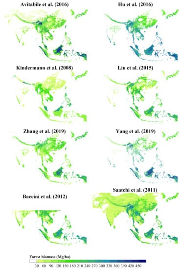
4.3. Southeast Asia
Saatchi et al. [19], Baccini et al. [18], Avitabile et al. [103] and Zhang and Liang [77] provided similar forest AGB spatial distributions across Southeast Asia, while Hu et al. [99] and Yang et al. [100] provided similar results especially in the tropical regions, where AGB was considerably higher than the other datasets (Figure 7). In southern China, AGB was less than 60 Mg/ha, the lowest among the eight forest datasets (Kindermann et al. [54]; Figure 7). Across southeast Asia, the majority of AGB estimates in Kindermann et al. [54] ranged from 30 to 120 Mg/ha, which was far from realistic (Figure 8). Additionally, there were substantial discrepancies in the spatial and frequency distribution between AGB from this dataset and from other datasets (Figure 7 and Figure 8). Similarly, differences between the Liu et al. [105] dataset and the others were also quite significant.
Figure 8 showed that among the eight forest AGB maps over Southeast Asia, the Avitabile et al. [103] and Zhang and Liang [77] datasets were quite similar, with the majority of AGB estimates from about 50 to 230 Mg/ha. The Avitabile et al. [103] dataset was generated by the fusion of the Saatchi et al. [19] and Baccini et al. [18] datasets using the bias removal and weighted linear averaging method, and should represent a more precise AGB map across the pan-tropical regions. The use of a similar method, also suggests more precise AGB estimates from the Zhang and Liang [77] dataset for Southeast Asia. The percentage curves of Hu et al. [99] and Baccini et al. [18] showed two peaks corresponding to AGB of about 150 Mg/ha and 300 Mg/ha, respectively. For the Yang et al. [100] dataset, most pixels had AGB of around 250 Mg/ha, and compared with other datasets, more pixels had AGB higher than 350 Mg/ha.
For evergreen broadleaf forests, AGB maps were spatially in agreement expect for the Kindermann et al. [54] and Yang et al. [100] datasets (Figure 9). However, in the mixed forest and especially in woody savannas, spatial differences in these AGB maps were evident. AGB for mixed forest in Baccini et al. [18] was quite different from other mixed forest maps, and there were large discrepancies between the Yang et al. [100] map and other datasets for woody savannas.
4.4. Tropical Africa
The Hu et al. [99] and Yang et al. [100] datasets had higher AGB than the other seven datasets shown in Figure 10 over tropical African forests, which was in agreement with comparable results in Southeast Asia. The majority of pixels had AGB > 280 Mg/ha, and few pixels had AGB < 180 Mg/ha, probably because both datasets used the MODIS land cover types to separate forest and non-forest, and the regions covered with woody savannas and savannas were masked (Figure 10 and Figure 11). The Liu et al. [105] dataset differed from others in AGB spatial and frequency distributions over tropical Africa. In the regions with higher AGB, the Baccini et al. [89] and Liu et al. [105] datasets had lower AGB compared to the other datasets (Figure 10). The Saatchi et al. [19] and Baccini et al. [18] datasets were both spatially and statistically similar, while the Zhang and Liang [77] dataset, although somewhat similar, had higher AGB in the high AGB regions. In accordance with Zhang and Liang [77], Hu et al. [99], and Yang et al. [100], the Avitabile et al. [103] dataset had higher AGB in the evergreen broadleaf forests (Figure 10 and Figure 12). However, as most of the tropical regions were covered with woody savannas and savannas and not evergreen broadleaf forests, the percentage curve (Figure 11) in Avitabile et al. [103] showed that most pixels had AGB < 50 Mg/ha due to lower AGB estimates for regions covered with woody savannas and savannas.
Statistical analysis of the spatial similarities and differences of these AGB datasets in different forest types showed that the nine AGB datasets in Figure 10 were spatially similar in evergreen broadleaf forests, but somewhat dissimilar in regions covered with woody savannas and savannas (Figure 12). In particular, the Hu et al. [99] and Yang et al. [100] datasets were quite different to other datasets in the woody savannas and savannas.
4.5. South America
Among the seven forest AGB datasets shown in Figure 13, the Kindermann et al. [54] dataset had the lowest AGB, while the Hu et al. [99] and Yang et al. [100] datasets had higher AGB than other datasets over almost all of South America. The higher AGB in Kindermann et al. [54] was mainly from 150 to 200 Mg/ha. The majority of pixels in the Yang et al. [100] and Hu et al. [99] maps had AGB of c. 290 and 320 Mg/ha, respectively. The Saatchi et al. [19], Avitabile et al. [103], and Zhang and Liang [77] datasets were somewhat consistent with one another, while the percentage curves revealed that only when AGB was > 200 Mg/ha, did they follow similar distributions (Figure 14). However, in regions where AGB was lower, most pixels in Zhang and Liang [77] ranged from 60 to 150 Mg/ha, higher than the corresponding 10~60 Mg/ha of Saatchi et al. [19] and 0~40 Mg/ha of Avitabile et al. [103], but much lower than the Kindermann et al. [54], Liu et al. [105], Hu et al. [99], and Yang et al. [100] datasets.
As was shown in the comparisons across Southeast Asia and tropical Africa, forest AGB datasets were spatially similar in evergreen broadleaf forest, but substantially different in the savannas across South America (Figure 15). The AGB in the Kindermann et al. [54] dataset was different from others, especially from Yang et al. [100] in evergreen broadleaf forest. While in the savannas, the Hu et al. [99] and Yang et al. [100] datasets were similar, but quite different from the others.
5. Limitations of Current AGB Maps and Future Improvements
5.1. Compilation of Field Biomass Data
The above efforts to generate accurate forest AGB maps mainly focus on the application of multiple datasets and advanced algorithms, while few efforts have been made to ensure the accuracy of field biomass data. Furthermore, the allometric equations used to calculate field biomass and the representativeness of field biomass are major sources of uncertainties of estimated AGB on a regional scale [112,113,114,115]. Additionally, most AGB maps are not validated due to lack of field biomass data. Therefore, the acquisition and compilation of abundant and highly accurate field biomass data, which would ensure the accuracy of biomass mapping, is of utmost importance.
Currently, researchers of several international networks such as RAINFOR (the Amazon Forest Inventory Network, http://www.rainfor.org/), AfriTRON (African Tropical Rainforest Observation Network, www.afritron.org), and ForestGEO (Global Earth Observatory, https://forestgeo.si.edu/) network, have engaged in utilizing long-term permanent sample plots to monitor forest biomass and dynamics [116]. The Forest Observation System (FOS, https://forest-observation-system.net/) which includes, but is not limited to data records from these networks, is tasked to coordinate in situ activities in relation to the BIOMASS mission [117]. The biomass plot data will be in unified format, and processed with standardized procedures. With the development of these international networks, sufficient field plots with acceptable accuracy will be available which would improve the calibration and validation of remotely sensed data-based biomass estimation on a large scale.
Previous studies indicate the possible limitations of using field plots for “truthing” due to the existence of plot biases and errors, particularly for heterogeneous landscapes [118]. Therefore, future forest biomass studies could use LiDAR as the sampling technique to complement to field-plot sampling.
5.2. Data Sources for Forest AGB Mapping
Although relationships between retrieved forest parameters and biomass have been demonstrated, their correlations vary in regions and are sometimes poor [119]. A full exploration of the relationships between forest biomass and its related parameters at different spatial resolutions as well as the associated factors influencing these relationships should be performed. The detailed relationships could be further utilized to improve the accuracy of AGB mapping.
Another limitation is that current AGB maps are retrieved mainly from optical data acquired by TM/ETM+ and MODIS sensors, which are known to saturate even at lower biomass and thus unable to acceptably capture high biomass values. The use of SAR and LiDAR data could help improve this problem to some degree, but currently, less than 1/3 of AGB maps are generated with a combination of field biomass, LiDAR data, optical and/or SAR data. The inclusion of SAR and LiDAR data should be fully considered for the future generation of biomass maps on a large scale [120]. Moreover, hyperspectral data look promising for improving the accuracy of biomass estimates, due to their capabilities of providing information on vegetation health and species composition [121,122]. The use of hyperspectral data in combination of other sensors in future studies should be considered to improve biomass mapping on a large scale.
5.3. Novel Approaches to Forest AGB Mapping
Current AGB maps retrieved from remotely sensed datasets mainly use GIS-based modelling methods based on some assumptions or empirical algorithms. Along with the development of machine learning algorithms, in particular deep learning algorithms, more advanced data-driven algorithms or a hybrid modelling that couples physical process models with data-driven machine learning could be considered in large-scale forest biomass mapping [123].
5.4. Accuracy Assessment
Uncertainties in AGB maps arise from uncertainties in sampling methods, modelling algorithms, datasets used, the choice of allometric equations, and the mismatch of field data and remotely sensed data [9]. Most AGB mapping studies have not fully quantified these uncertainties. The methods used for quantifying mapping uncertainties include the Monte Carlo error propagation approach [66,83,124], bootstrap techniques [97], confidence intervals [78,125], and model-based estimators [86,87]. However, these published studies have only partially quantified uncertainties in the estimation, more effective and efficient methods to express and quantify uncertainty in all its forms are needed [126,127]. Moreover, the uncertainty caused by temporal mismatches in datasets has often been ignored. Since studies use field data to calibrate remotely sensed datasets, temporal mismatches between measured field data and predictors could lead to uncertainties in estimated biomass. Comprehensively addressing more sources of uncertainty would help to better understand the accuracy of generated biomass maps and further promote the application of biomass maps in related fields.
5.5. Forest Biomass Dynamics
Although many algorithms have been developed to detect trends or monitor forests, few can be directly used to estimate biomass changes or dynamics [128,129]. Quantifying forest biomass dynamics remains a challenging task. One reason is that current biomass maps have inherently large uncertainties, and the discrepancies in biomass estimates could be even larger than the actual changes in the forest AGB [110]. A further reason is that forest biomass is changing due to intervening disturbance and growth [23,130,131,132]. Much efforts have been made on the detection of disturbances, but little is known about the biomass losses and gains due to these disturbances and the following recovery from disturbances. From a dataset perspective focused on the study of forest biomass dynamics, long-term permanent plot data cannot be applied to large areas due to adequate sampling constraints, while remotely sensed data can detect forest area changes but remain less capable of detecting forest carbon density, especially where the changes is subtle [118,133,134]. To infer forest AGB dynamics accurately in the future, we should on one hand continue to improve accuracy of biomass estimates, and on the other hand, broaden our knowledge of biomass losses and gains due to all kinds of disturbance and recovery.
6. Conclusions
In this paper, we reviewed the existing regional and global forest AGB maps, including five maps obtained through GIS-based modelling; sixteen maps produced by integrating field biomass data directly with optical and/or radar data; five high-resolution maps retrieved from field biomass data and LiDAR data; fourteen maps generated from a combination of field data, LiDAR data, and optical and/or radar data; and seven maps generated or regenerated using existing biomass datasets. In spite of numerous efforts to map the spatial distribution of forest AGB with a variety of datasets and advanced methods, current AGB maps still contain large uncertainties. Comparison of biomass datasets across Europe, the conterminous United States, Southeast Asia, tropical Africa and South America, suggested that they were almost entirely inconsistent, particularly in woody savannas and savannas. The uncertainties in AGB maps could be from the allometric equations used to calculate field data, the choice and quality of remotely sensed data, as well as the algorithms to map forest biomass or extrapolation techniques, but have not been fully quantified. We suggest the future directions for generating more accurate large-scale forest biomass maps should concentrate on the compilation of field biomass data, novel approaches of forest biomass mapping, and comprehensively addressing the accuracy of generated biomass maps.
Funding
This work was supported by the National Natural Science Foundation of China (Grant No. 41801347), the National Key Research and Development Program of China (No. 2016YFA0600103), and the Fundamental Research Funds for the Central Universities (FRF-TP-17-041A1).
Conflicts of Interest
The authors declare no conflicts of interest.
References
- Canadell, J.G.; Raupach, M.R. Managing forests for climate change mitigation. Science 2008, 320, 1456–1457. [Google Scholar] [CrossRef] [PubMed]
- Luyssaert, S.; Schulze, E.D.; Borner, A.; Knohl, A.; Hessenmoller, D.; Law, B.E.; Ciais, P.; Grace, J. Old-growth forests as global carbon sinks. Nature 2008, 455, 213–215. [Google Scholar] [CrossRef] [PubMed]
- Kumar, L.; Mutanga, O. Remote Sensing of Above-Ground Biomass. Remote Sens. 2017, 9, 935. [Google Scholar] [CrossRef]
- Kim, D.-H.; Kim, J.-H.; Park, J.-H.; Ewane, E.B.; Lee, D.-H. Correlation between above-ground and below-ground biomass of 13-year-old Pinus densiflora S. et Z. planted in a post-fire area in Samcheok. For. Sci. Technol. 2016, 12, 115–124. [Google Scholar]
- Saatchi, S.S.; Houghton, R.A.; Dos Santos Alvalá, R.C.; Soares, J.V.; Yu, Y. Distribution of aboveground live biomass in the Amazon basin. Glob. Chang. Biol. 2007, 13, 816–837. [Google Scholar] [CrossRef]
- Ketterings, Q.M.; Coe, R.; van Noordwijk, M.; Ambagau’, Y.; Palm, C.A. Reducing uncertainty in the use of allometric biomass equations for predicting above-ground tree biomass in mixed secondary forests. For. Ecol. Manag. 2001, 146, 199–209. [Google Scholar] [CrossRef]
- Fang, J.; Chen, A.; Peng, C.; Zhao, S.; Ci, L. Changes in Forest Biomass Carbon Storage in China Between 1949 and 1998. Science 2001, 292, 2320–2322. [Google Scholar] [CrossRef]
- Fang, J.; Guo, Z.; Hu, H.; Kato, T.; Muraoka, H.; Son, Y. Forest biomass carbon sinks in East Asia, with special reference to the relative contributions of forest expansion and forest growth. Glob. Chang. Biol. 2014, 20, 2019–2030. [Google Scholar] [CrossRef]
- Lu, D.; Chen, Q.; Wang, G.; Liu, L.; Li, G.; Moran, E. A survey of remote sensing-based aboveground biomass estimation methods in forest ecosystems. Int. J. Digit. Earth 2016, 9, 63–105. [Google Scholar] [CrossRef]
- Powell, S.L.; Cohen, W.B.; Healey, S.P.; Kennedy, R.E.; Moisen, G.G.; Pierce, K.B.; Ohmann, J.L. Quantification of live aboveground forest biomass dynamics with Landsat time-series and field inventory data: A comparison of empirical modeling approaches. Remote Sens. Environ. 2010, 114, 1053–1068. [Google Scholar] [CrossRef]
- Sinha, S.; Jeganathan, C.; Sharma, L.K.; Nathawat, M.S. A review of radar remote sensing for biomass estimation. Int. J. Environ. Sci. Technol. 2015, 12, 1779–1792. [Google Scholar] [CrossRef]
- Lim, K.; Treitz, P.; Wulder, M.; St-Onge, B.; Flood, M. LiDAR remote sensing of forest structure. Prog. Phys. Geog. 2003, 27, 88–106. [Google Scholar] [CrossRef]
- Tian, X.; Yan, M.; van der Tol, C.; Li, Z.; Su, Z.; Chen, E.; Li, X.; Li, L.; Wang, X.; Pan, X.; et al. Modeling forest above-ground biomass dynamics using multi-source data and incorporated models: A case study over the qilian mountains. Agric. For. Meteorol. 2017, 246, 1–14. [Google Scholar] [CrossRef]
- Hurtt, G.C.; Fisk, J.; Thomas, R.Q.; Dubayah, R.; Moorcroft, P.R.; Shugart, H.H. Linking models and data on vegetation structure. J. Geophys. Res. Biogeosci. 2010, 115, G00E10. [Google Scholar] [CrossRef]
- Waring, R.H.; Coops, N.C.; Landsberg, J.J. Improving predictions of forest growth using the 3-PGS model with observations made by remote sensing. For. Ecol. Manag. 2010, 259, 1722–1729. [Google Scholar] [CrossRef]
- Zolkos, S.G.; Goetz, S.J.; Dubayah, R. A meta-analysis of terrestrial aboveground biomass estimation using lidar remote sensing. Remote Sens. Environ. 2013, 128, 289–298. [Google Scholar] [CrossRef]
- Goetz, S.; Baccini, A.; Laporte, N.; Johns, T.; Walker, W.; Kellndorfer, J.; Houghton, R.; Sun, M. Mapping and monitoring carbon stocks with satellite observations: A comparison of methods. Carbon Balance Manag. 2009, 4, 2. [Google Scholar] [CrossRef]
- Baccini, A.; Goetz, S.J.; Walker, W.S.; Laporte, N.T.; Sun, M.; Sulla-Menashe, D.; Hackler, J.; Beck, P.S.A.; Dubayah, R.; Friedl, M.A.; et al. Estimated carbon dioxide emissions from tropical deforestation improved by carbon-density maps. Nat. Clim. Chang. 2012, 2, 182–185. [Google Scholar] [CrossRef]
- Saatchi, S.S.; Harris, N.L.; Brown, S.; Lefsky, M.; Mitchard, E.T.A.; Salas, W.; Zutta, B.R.; Buermann, W.; Lewis, S.L.; Hagen, S.; et al. Benchmark map of forest carbon stocks in tropical regions across three continents. Proc. Natl. Acad. Sci. USA 2011, 108, 9899–9904. [Google Scholar] [CrossRef]
- Carvalhais, N.; Forkel, M.; Khomik, M.; Bellarby, J.; Jung, M.; Migliavacca, M.; Mu, M.; Saatchi, S.; Santoro, M.; Thurner, M.; et al. Global covariation of carbon turnover times with climate in terrestrial ecosystems. Nature 2014, 514, 213–217. [Google Scholar] [CrossRef]
- Langner, A.; Achard, F.; Grassi, G. Can recent pan-tropical biomass maps be used to derive alternative Tier 1 values for reporting REDD+ activities under UNFCCC? Environ. Res. Lett. 2014, 9, 124008. [Google Scholar] [CrossRef]
- Zhang, Y.; Liang, S. Surface radiative forcing of forest disturbances over northeastern China. Environ. Res. Lett. 2014, 9, 024002. [Google Scholar] [CrossRef]
- Zhang, Y.; Liang, S. Changes in forest biomass and linkage to climate and forest disturbances over Northeastern China. Glob. Chang. Biol. 2014, 20, 2596–2606. [Google Scholar] [CrossRef] [PubMed]
- Lu, D. The potential and challenge of remote sensing-based biomass estimation. Int. J. Remote Sens. 2006, 27, 1297–1328. [Google Scholar] [CrossRef]
- Koch, B. Status and future of laser scanning, synthetic aperture radar and hyperspectral remote sensing data for forest biomass assessment. ISPRS J. Photogramm. 2010, 65, 581–590. [Google Scholar] [CrossRef]
- Lucas, R.M.; Mitchell, A.L.; Armston, J. Measurement of Forest Above-Ground Biomass Using Active and Passive Remote Sensing at Large (Subnational to Global) Scales. Curr. For. Rep. 2015, 1, 162–177. [Google Scholar] [CrossRef]
- Chave, J.; Andalo, C.; Brown, S.; Cairns, M.A.; Chambers, J.Q.; Eamus, D.; Fölster, H.; Fromard, F.; Higuchi, N.; Kira, T. Tree allometry and improved estimation of carbon stocks and balance in tropical forests. Oecologia 2005, 145, 87–99. [Google Scholar] [CrossRef]
- Wu, X.; Wang, X.; Wu, Y.; Xia, X.; Fang, J. Forest biomass is strongly shaped by forest height across boreal to tropical forests in China. J. Plant Ecol. 2015, 8, 559–567. [Google Scholar] [CrossRef]
- Solberg, S.; Næsset, E.; Gobakken, T.; Bollandsås, O.-M. Forest biomass change estimated from height change in interferometric SAR height models. Carbon Balance Manag. 2014, 9, 5. [Google Scholar] [CrossRef]
- Yu, Y.; Saatchi, S.; Heath, L.S.; LaPoint, E.; Myneni, R.; Knyazikhin, Y. Regional distribution of forest height and biomass from multisensor data fusion. J. Geophys. Res. Biogeosci. 2010, 115, G00E12. [Google Scholar] [CrossRef]
- Palace, M.W.; Sullivan, F.B.; Ducey, M.J.; Treuhaft, R.N.; Herrick, C.; Shimbo, J.Z.; Mota-E-Silva, J. Estimating forest structure in a tropical forest using field measurements, a synthetic model and discrete return lidar data. Remote Sens. Environ. 2015, 161, 1–11. [Google Scholar] [CrossRef]
- Zhang, G.; Ganguly, S.; Nemani, R.R.; White, M.A.; Milesi, C.; Hashimoto, H.; Wang, W.; Saatchi, S.; Yu, Y.; Myneni, R.B. Estimation of forest aboveground biomass in California using canopy height and leaf area index estimated from satellite data. Remote Sens. Environ. 2014, 151, 44–56. [Google Scholar] [CrossRef]
- Zhang, X.; Kondragunta, S. Estimating forest biomass in the USA using generalized allometric models and MODIS land products. Geophys. Res. Lett. 2006, 33, L09402. [Google Scholar] [CrossRef] [Green Version]
- Berner, L.T.; Law, B.E. Plant traits, productivity, biomass and soil properties from forest sites in the Pacific Northwest, 1999–2014. Sci. Data 2016, 3, 160002. [Google Scholar] [CrossRef] [Green Version]
- Zhang, H.; Wang, K.; Xu, X.; Song, T.; Xu, Y.; Zeng, F. Biogeographical patterns of biomass allocation in leaves, stems, and roots in China’s forests. Sci. Rep. 2015, 5, 15997. [Google Scholar] [CrossRef] [Green Version]
- Keeling, H.C.; Phillips, O.L. The global relationship between forest productivity and biomass. Glob. Ecol. Biogeogr. 2007, 16, 618–631. [Google Scholar] [CrossRef]
- Ernest, S.K.M.; Enquist, B.J.; Brown, J.H.; Charnov, E.L.; Gillooly, J.F.; Savage, V.M.; White, E.P.; Smith, F.A.; Hadly, E.A.; Haskell, J.P.; et al. Thermodynamic and metabolic effects on the scaling of production and population energy use. Ecol. Lett. 2003, 6, 990–995. [Google Scholar] [CrossRef] [Green Version]
- Hui, D.; Wang, J.; Le, X.; Shen, W.; Ren, H. Influences of biotic and abiotic factors on the relationship between tree productivity and biomass in China. For. Ecol. Manag. 2012, 264, 72–80. [Google Scholar] [CrossRef]
- Tian, F.; Brandt, M.; Liu, Y.Y.; Verger, A.; Tagesson, T.; Diouf, A.A.; Rasmussen, K.; Mbow, C.; Wang, Y.; Fensholt, R. Remote sensing of vegetation dynamics in drylands: Evaluating vegetation optical depth (VOD) using AVHRR NDVI and in situ green biomass data over West African Sahel. Remote Sens. Environ. 2016, 177, 265–276. [Google Scholar] [CrossRef] [Green Version]
- Garroutte, E.L.; Hansen, A.J.; Lawrence, R.L. Using NDVI and EVI to Map Spatiotemporal Variation in the Biomass and Quality of Forage for Migratory Elk in the Greater Yellowstone Ecosystem. Remote Sens. 2016, 8, 404. [Google Scholar] [CrossRef] [Green Version]
- Durante, P.; Martín-Alcón, S.; Gil-Tena, A.; Algeet, N.; Tomé, J.L.; Recuero, L.; Palacios-Orueta, A.; Oyonarte, C. Improving Aboveground Forest Biomass Maps: From High-Resolution to National Scale. Remote Sens. 2019, 11, 795. [Google Scholar] [CrossRef] [Green Version]
- Chen, J.M. Evaluation of Vegetation Indices and a Modified Simple Ratio for Boreal Applications. Can. J. Remote Sens. 1996, 22, 229–242. [Google Scholar] [CrossRef]
- Liu, Y.Y.; van Dijk, A.I.J.M.; McCabe, M.F.; Evans, J.P.; de Jeu, R.A.M. Global vegetation biomass change (1988–2008) and attribution to environmental and human drivers. Glob. Ecol. Biogeogr. 2013, 22, 692–705. [Google Scholar] [CrossRef]
- Blackard, J.A.; Finco, M.V.; Helmer, E.H.; Holden, G.R.; Hoppus, M.L.; Jacobs, D.M.; Lister, A.J.; Moisen, G.G.; Nelson, M.D.; Riemann, R.; et al. Mapping, U.S. forest biomass using nationwide forest inventory data and moderate resolution information. Remote Sens. Environ. 2008, 112, 1658–1677. [Google Scholar] [CrossRef]
- Hansen, M.C.; Potapov, P.V.; Moore, R.; Hancher, M.; Turubanova, S.A.; Tyukavina, A.; Thau, D.; Stehman, S.V.; Goetz, S.J.; Loveland, T.R.; et al. High-Resolution Global Maps of 21st-Century Forest Cover Change. Science 2013, 342, 850–853. [Google Scholar] [CrossRef] [PubMed] [Green Version]
- McEwan, R.W.; Lin, Y.-C.; Sun, I.F.; Hsieh, C.-F.; Su, S.-H.; Chang, L.-W.; Song, G.-Z.M.; Wang, H.-H.; Hwong, J.-L.; Lin, K.-C.; et al. Topographic and biotic regulation of aboveground carbon storage in subtropical broad-leaved forests of Taiwan. For. Ecol. Manag. 2011, 262, 1817–1825. [Google Scholar] [CrossRef]
- Frolking, S.; Palace, M.W.; Clark, D.B.; Chambers, J.Q.; Shugart, H.H.; Hurtt, G.C. Forest disturbance and recovery: A general review in the context of spaceborne remote sensing of impacts on aboveground biomass and canopy structure. J. Geophys. Res. Biogeosci. 2009, 114, G00E02. [Google Scholar] [CrossRef]
- Asner, G.P.; Flint Hughes, R.; Varga, T.A.; Knapp, D.E.; Kennedy-Bowdoin, T. Environmental and Biotic Controls over Aboveground Biomass Throughout a Tropical Rain Forest. Ecosystems 2009, 12, 261–278. [Google Scholar] [CrossRef]
- Ruesch, A.S.; Gibbs, H.K. New IPCC Tier-1 Global Biomass Carbon Map For the Year 2000. Carbon Dioxide Information Analysis Center, 2008. Available online: http://cdiac.ornl.gov (accessed on 13 September 2017).
- IPCC. 2006 IPCC Guidelines for National Greenhouse Gas Inventories; Institute for Global Environmental Strategies: Hayama, Japan, 2006. [Google Scholar]
- Barredo, J.I.; San-Miguel-Ayanz, J.; Caudullo, G.; Busetto, L. A European Map of Living Forest Biomass and Carbon Stock; EUR–Scientific and Technical Research; Joint Research Centre of the European Commission: Ispra, Italy, 2012; p. 25730. [Google Scholar]
- FAO. Global Forest Resources Assessment 2010: Main Report; Food and Agriculture Organization of the United Nations: Rome, Italy, 2010. [Google Scholar]
- Hengeveld, G.M.; Gunia, K.; Didion, M.; Zudin, S.; Clerkx, A.P.P.M.; Schelhaas, M.J. Global 1-degree Maps of Forest Area, Carbon Stocks, and Biomass, 1950-2010; ORNL DAAC: Oak Ridge, TN, USA, 2015. [CrossRef]
- Kindermann, G.E.; McCallum, I.; Fritz, S.; Obersteiner, M. A global forest growing stock, biomass and carbon map based on FAO statistics. Silva Fenn. 2008, 42, 387–396. [Google Scholar] [CrossRef] [Green Version]
- Brown, S.; Gaston, G. Tropical Africa: Land Use, Biomass, and Carbon Estimates for 1980: NDP-055; Carbon Dioxide Information Center, Oak Ridge National Laboratory: Oak Rigde, TN, USA, 2001; revised for the web 2001.
- Brown, S.L.; Iverson, L.R.; Prasad, A.M.; Beaty, T.W. Geographical Distribution of Biomass Carbon in Tropical Southeast Asian Forests: A Database; Carbon Dioxide Information Center, Environmental Sciences Division, Oak Ridge National Laboratory: Oak Ridge, TN, USA, 2001.
- Gibbs, H.; Brown, S. Geographical Distribution of Woody Biomass Carbon Stocks in Tropical Africa: An Updated Database for 2000; Carbon Dioxide Information Center, Oak Ridge National Laboratory: Oak Ridge, TN, USA, 2007. Available online: http://cdiac.ornl.gov/epubs/ndp/ndp055/ndp055b.html (accessed on 19 November 2014).
- Gibbs, H.K.; Brown, S. Geographical Distribution of Biomass Carbon in Tropical Southeast Asian Forests: An Updated Database for 2000; Carbon Dioxide Information Center, Oak Ridge National Laboratory: Oak Ridge, TN, USA, 2007. Available online: http://cdiac.ornl.gov/epubs/ndp/ndp068/ndp068b.html (accessed on 19 November 2014).
- Kellndorfer, J.; Walker, W.; Kirsch, K.; Fiske, G.; Bishop, J.; LaPoint, L.; Hoppus, M.; Westfall, J. NACP Aboveground Biomass and Carbon Baseline Data, V. 2 (NBCD 2000); ORNL DAAC: Oak Ridge, TN, USA, 2013. [CrossRef]
- Hardiman, B.S.; Wang, J.A.; Hutyra, L.R.; Gately, C.K.; Getson, J.M.; Friedl, M.A. Accounting for urban biogenic fluxes in regional carbon budgets. Sci. Total Environ. 2017, 592, 366–372. [Google Scholar] [CrossRef]
- Raciti, S.M.; Hutyra, L.R.; Newell, J.D. Mapping carbon storage in urban trees with multi-source remote sensing data: Relationships between biomass, land use, and demographics in Boston neighborhoods. Sci. Total Environ. 2014, 500, 72–83. [Google Scholar] [CrossRef] [PubMed]
- Rodriguez-Veiga, P.; Quegan, S.; Carreiras, J.; Persson, H.J.; Fransson, J.E.S.; Hoscilo, A.; Ziolkowski, D.; Sterenczak, K.; Lohberger, S.; Staengel, M.; et al. Forest biomass retrieval approaches from earth observation in different biomes. Int. J. Appl. Earth Obs. 2019, 77, 53–68. [Google Scholar] [CrossRef]
- Wilson, B.T.; Woodall, C.; Griffith, D. Imputing forest carbon stock estimates from inventory plots to a nationally continuous coverage. Carbon Balance Manag. 2013, 8, 1. [Google Scholar] [CrossRef] [Green Version]
- Ji, L.; Wylie, B.K.; Nossov, D.R.; Peterson, B.; Waldrop, M.P.; McFarland, J.W.; Rover, J.; Hollingsworth, T.N. Estimating aboveground biomass in interior Alaska with Landsat data and field measurements. Int. J. Appl. Earth Obs. 2012, 18, 451–461. [Google Scholar] [CrossRef]
- Cartus, O.; Kellndorfer, J.; Walker, W.; Franco, C.; Bishop, J.; Santos, L.; Fuentes, J. A National, Detailed Map of Forest Aboveground Carbon Stocks in Mexico. Remote Sens. 2014, 6, 5559–5588. [Google Scholar] [CrossRef] [Green Version]
- Rodríguez-Veiga, P.; Saatchi, S.; Tansey, K.; Balzter, H. Magnitude, spatial distribution and uncertainty of forest biomass stocks in Mexico. Remote Sens. Environ. 2016, 183, 265–281. [Google Scholar] [CrossRef] [Green Version]
- Le Toan, T.; Quegan, S.; Davidson, M.W.J.; Balzter, H.; Paillou, P.; Papathanassiou, K.; Plummer, S.; Rocca, F.; Saatchi, S.; Shugart, H.; et al. The BIOMASS mission: Mapping global forest biomass to better understand the terrestrial carbon cycle. Remote Sens. Environ. 2011, 115, 2850–2860. [Google Scholar] [CrossRef] [Green Version]
- Beaudoin, A.; Bernier, P.Y.; Guindon, L.; Villemaire, P.; Guo, X.J.; Stinson, G.; Bergeron, T.; Magnussen, S.; Hall, R.J. Mapping attributes of Canada’s forests at moderate resolution through kNN and MODIS imagery. Can. J. For. Res. 2014, 44, 521–532. [Google Scholar] [CrossRef] [Green Version]
- Beaudoin, A.; Bernier, P.Y.; Villemaire, P.; Guindon, L.; Guo, X.J. Tracking forest attributes across Canada between 2001 and 2011 using a k nearest neighbors mapping approach applied to MODIS imagery. Can. J. For. Res. 2017, 48, 85–93. [Google Scholar] [CrossRef] [Green Version]
- Gallaun, H.; Zanchi, G.; Nabuurs, G.-J.; Hengeveld, G.; Schardt, M.; Verkerk, P.J. EU-wide maps of growing stock and above-ground biomass in forests based on remote sensing and field measurements. For. Ecol. Manag. 2010, 260, 252–261. [Google Scholar] [CrossRef]
- Houghton, R.A.; Butman, D.; Bunn, A.G.; Krankina, O.N.; Schlesinger, P.; Stone, T.A. Mapping Russian forest biomass with data from satellites and forest inventories. Environ. Res. Lett. 2007, 2, 045032. [Google Scholar] [CrossRef]
- Yin, G.; Zhang, Y.; Sun, Y.; Wang, T.; Zeng, Z.; Piao, S. MODIS Based Estimation of Forest Aboveground Biomass in China. PLoS ONE 2015, 10, e0130143. [Google Scholar] [CrossRef] [Green Version]
- Du, L.; Zhou, T.; Zou, Z.; Zhao, X.; Huang, K.; Wu, H. Mapping Forest Biomass Using Remote Sensing and National Forest Inventory in China. Forests 2014, 5, 1267–1283. [Google Scholar] [CrossRef] [Green Version]
- Saatchi, S.; Malhi, Y.; Zutta, B.; Buermann, W.; Anderson, L.O.; Araujo, A.M.; Phillips, O.L.; Peacock, J.; ter Steege, H.; Lopez Gonzalez, G.; et al. Mapping landscape scale variations of forest structure, biomass, and productivity in Amazonia. Biogeosci. Discuss. 2009, 6, 5461–5505. [Google Scholar] [CrossRef] [Green Version]
- Avtar, R.; Suzuki, R.; Takeuchi, W.; Sawada, H. PALSAR 50 m Mosaic Data Based National Level Biomass Estimation in Cambodia for Implementation of REDD+ Mechanism. PLoS ONE 2013, 8, e74807. [Google Scholar] [CrossRef] [PubMed]
- Anaya, J.A.; Chuvieco, E.; Palacios-Orueta, A. Aboveground biomass assessment in Colombia: A remote sensing approach. For. Ecol. Manag. 2009, 257, 1237–1246. [Google Scholar] [CrossRef]
- Zhang, Y.; Liang, S. A new high-resolution global forest above-ground biomass map in 2000s by integrating comprehensive reference datasets with multiple high-level satellite products. Int. J. Appl. Earth Obs. 2019. submitted. [Google Scholar]
- Cook, B.D.; Swatantran, A.; Duncanson, L.; Armstrong, A.; Pinto, N.; Nelson, R.F. CMS: LiDAR-derived Estimates of Aboveground Biomass at Four Forested Sites, USA; ORNL Distributed Active Archive Center: Oak Ridge, TN, USA, 2014. [CrossRef]
- Babcock, C.; Finley, A.O.; Cook, B.D.; Weiskittel, A.; Woodall, C.W. CMS: Aboveground Biomass from Penobscot Experimental Forest, Maine, 2012; ORNL Distributed Active Archive Center: Oak Ridge, TN, USA, 2016. [CrossRef]
- Babcock, C.; Finley, A.O.; Cook, B.D.; Weiskittel, A.; Woodall, C.W. Modeling forest biomass and growth: Coupling long-term inventory and LiDAR data. Remote Sens. Environ. 2016, 182, 1–12. [Google Scholar] [CrossRef] [Green Version]
- Dubayah, R.O.; Swatantran, A.; Huang, W.; Duncanson, L.; Johnson, K.; Tang, H.; Dunne, J.O.; Hurtt, G.C. CMS: LiDAR-derived Aboveground Biomass, Canopy Height and Cover for Maryland, 2011; ORNL Distributed Active Archive Center: Oak Ridge, TN, USA, 2016. [CrossRef]
- Dubayah, R.O.; Swatantran, A.; Huang, W.; Duncanson, L.; Tang, H.; Johnson, K.; Dunne, J.O.; Hurtt, G.C. CMS: LiDAR-derived Biomass, Canopy Height and Cover, Sonoma County, California, 2013; ORNL Distributed Active Archive Center: Oak Ridge, TN, USA, 2017. [CrossRef]
- Xu, Q.; Man, A.; Fredrickson, M.; Hou, Z.; Pitkänen, J.; Wing, B.; Ramirez, C.; Li, B.; Greenberg, J.A. Quantification of uncertainty in aboveground biomass estimates derived from small-footprint airborne LiDAR. Remote Sens. Environ. 2018, 216, 514–528. [Google Scholar] [CrossRef]
- Xu, Q.; Greenberg, J. LiDAR-Derived Aboveground Biomass and Uncertainty for California Forests, 2005–2014; ORNL Distributed Active Archive Center: Oak Ridge, TN, USA, 2018. [CrossRef]
- Neigh, C.S.; Nelson, R.F.; Ranson, K.J.; Margolis, H.; Montesano, P.M.; Sun, G.; Kharuk, V.; Naesset, E.; Wulder, M.A.; Anderson, H. LiDAR-based Biomass Estimates, Boreal Forest Biome, Eurasia, 2005–2006; ORNL DAAC: Oak Ridge, TN, USA, 2015.
- Neigh, C.S.R.; Nelson, R.F.; Ranson, K.J.; Margolis, H.A.; Montesano, P.M.; Sun, G.; Kharuk, V.; Næsset, E.; Wulder, M.A.; Andersen, H.-E. Taking stock of circumboreal forest carbon with ground measurements, airborne and spaceborne LiDAR. Remote Sens. Environ. 2013, 137, 274–287. [Google Scholar] [CrossRef] [Green Version]
- Ståhl, G.; Holm, S.; Gregoire, T.G.; Gobakken, T.; Næsset, E.; Nelson, R. Model-based inference for biomass estimation in a LiDAR sample survey in Hedmark County, Norway. Can. J. For. Res. 2011, 41, 96–107. [Google Scholar] [CrossRef] [Green Version]
- Margolis, H.; Sun, G.; Montesano, P.M.; Nelson, R.F. NACP LiDAR-based Biomass Estimates, Boreal Forest Biome, North America, 2005-2006; ORNL Distributed Active Archive Center: Oak Ridge, TN, USA, 2015.
- Baccini, A.; Laporte, N.; Goetz, S.J.; Sun, M.; Dong, H. A first map of tropical Africa’s above-ground biomass derived from satellite imagery. Environ. Res. Lett. 2008, 3, 045011. [Google Scholar] [CrossRef] [Green Version]
- Mitchard, E.T.A.; Saatchi, S.S.; Lewis, S.L.; Feldpausch, T.R.; Gerard, F.F.; Woodhouse, I.H.; Meir, P. Comment on A first map of tropical Africa’s above-ground biomass derived from satellite imagery. Environ. Res. Lett. 2011, 6, 49001–49006. [Google Scholar] [CrossRef]
- Baccini, A.; Walker, W.; Farina, M.; Houghton, R.A. CMS: Estimated Deforested Area Biomass, Tropical America, Africa, and Asia, 2000; ORNL Distributed Active Archive Center: Oak Ridge, TN, USA, 2016. [CrossRef]
- Asner, G.P.; Mascaro, J.; Anderson, C.; Knapp, D.E.; Martin, R.E.; Kennedy-Bowdoin, T.; van Breugel, M.; Davies, S.; Hall, J.S.; Muller-Landau, H.C.; et al. High-fidelity national carbon mapping for resource management and REDD+. Carbon Balance Manag. 2013, 8, 7. [Google Scholar] [CrossRef] [Green Version]
- Asner, G.P.; Knapp, D.E.; Martin, R.E.; Tupayachi, R.; Anderson, C.B.; Mascaro, J.; Sinca, F.; Chadwick, K.D.; Higgins, M.; Farfan, W.; et al. Targeted carbon conservation at national scales with high-resolution monitoring. Proc. Natl. Acad. Sci. USA 2014, 111, E5016–E5022. [Google Scholar] [CrossRef] [Green Version]
- Fayad, I.; Baghdadi, N.; Guitet, S.; Bailly, J.-S.; Hérault, B.; Gond, V.; El Hajj, M.; Tong Minh, D.H. Aboveground biomass mapping in French Guiana by combining remote sensing, forest inventories and environmental data. Int. J. Appl. Earth Obs. 2016, 52, 502–514. [Google Scholar] [CrossRef] [Green Version]
- Vieilledent, G.; Gardi, O.; Grinand, C.; Burren, C.; Andriamanjato, M.; Camara, C.; Gardner, C.J.; Glass, L.; Rasolohery, A.; Ratsimba, H.R. Bioclimatic envelope models predict a decrease in tropical forest carbon stocks with climate change in Madagascar. J. Ecol. 2016, 104, 703–715. [Google Scholar] [CrossRef] [Green Version]
- Hajj, M.E.; Baghdadi, N.; Fayad, I.; Vieilledent, G.; Bailly, J.-S.; Minh, D.H.T. Interest of Integrating Spaceborne LiDAR Data to Improve the Estimation of Biomass in High Biomass Forested Areas. Remote Sens. 2017, 9, 213. [Google Scholar] [CrossRef] [Green Version]
- Zhang, Y.; Liang, S.; Sun, G. Forest biomass mapping of Northeastern China Using GLAS and MODIS Data. IEEE J. Sel. Top. Appl. Earth Obs. Remote Sens. 2014, 7, 140–152. [Google Scholar] [CrossRef]
- Su, Y.; Guo, Q.; Xue, B.; Hu, T.; Alvarez, O.; Tao, S.; Fang, J. Spatial distribution of forest aboveground biomass in China: Estimation through combination of spaceborne lidar, optical imagery, and forest inventory data. Remote Sens. Environ. 2016, 173, 187–199. [Google Scholar] [CrossRef] [Green Version]
- Hu, T.; Su, Y.; Xue, B.; Liu, J.; Zhao, X.; Fang, J.; Guo, Q. Mapping Global Forest Aboveground Biomass with Spaceborne LiDAR, Optical Imagery, and Forest Inventory Data. Remote Sens. 2016, 8, 565. [Google Scholar] [CrossRef] [Green Version]
- Yang, L.; Liang, S.; Zhang, Y. A new method for generating a global forest aboveground biomass map from multiple high-level satellite products and ancillary information. IEEE J. Sel. Top. Appl. Earth Obs. Remote Sens. 2019. Submitted. [Google Scholar]
- Santoro, M.; Beaudoin, A.; Beer, C.; Cartus, O.; Fransson, J.E.S.; Hall, R.J.; Pathe, C.; Schmullius, C.; Schepaschenko, D.; Shvidenko, A.; et al. Forest growing stock volume of the northern hemisphere: Spatially explicit estimates for 2010 derived from Envisat ASAR. Remote Sens. Environ. 2015, 168, 316–334. [Google Scholar] [CrossRef]
- Thurner, M.; Beer, C.; Santoro, M.; Carvalhais, N.; Wutzler, T.; Schepaschenko, D.; Shvidenko, A.; Kompter, E.; Ahrens, B.; Levick, S.R.; et al. Carbon stock and density of northern boreal and temperate forests. Glob. Ecol. Biogeogr. 2014, 23, 297–310. [Google Scholar] [CrossRef]
- Avitabile, V.; Herold, M.; Heuvelink, G.B.M.; Lewis, S.L.; Phillips, O.L.; Asner, G.P.; Armston, J.; Ashton, P.S.; Banin, L.; Bayol, N.; et al. An integrated pan-tropical biomass map using multiple reference datasets. Glob. Chang. Biol. 2016, 22, 1406–1420. [Google Scholar] [CrossRef] [PubMed] [Green Version]
- Englund, O.; Sparovek, G.; Berndes, G.; Freitas, F.; Ometto, J.P.; Oliveira, P.V.D.C.E.; Costa Jr, C.; Lapola, D. A new high-resolution nationwide aboveground carbon map for Brazil. Geo Geogr. Environ. 2017, 4, e00045. [Google Scholar] [CrossRef] [Green Version]
- Liu, Y.Y.; van Dijk, A.I.J.M.; de Jeu, R.A.M.; Canadell, J.G.; McCabe, M.F.; Evans, J.P.; Wang, G. Recent reversal in loss of global terrestrial biomass. Nat. Clim. Chang. 2015, 5, 470–474. [Google Scholar] [CrossRef]
- Rödig, E.; Cuntz, M.; Heinke, J.; Rammig, A.; Huth, A. Spatial heterogeneity of biomass and forest structure of the Amazon rain forest: Linking remote sensing, forest modelling and field inventory. Glob. Ecol. Biogeogr. 2017, 26, 1292–1302. [Google Scholar] [CrossRef]
- Busetto, L.; Barredo, J.I.; Sanmiguelayanz, J. Developing a Spatially-Explicit Pan-European Dataset of Forest Biomass Increment. In Proceedings of the 22nd European Biomass Conference and Exhibition, Hamburg, Germany, 23–26 June 2014. [Google Scholar]
- Avitabile, V.; Herold, M.; Henry, M.; Schmullius, C. Mapping biomass with remote sensing: A comparison of methods for the case study of Uganda. Carbon Balance Manag. 2011, 6, 7. [Google Scholar] [CrossRef] [Green Version]
- Neeti, N.; Kennedy, R. Comparison of national level biomass maps for conterminous US: Understanding pattern and causes of differences. Carbon Balance Manag. 2016, 11, 19. [Google Scholar] [CrossRef] [PubMed] [Green Version]
- Mitchard, E.; Saatchi, S.; Baccini, A.; Asner, G.; Goetz, S.; Harris, N.; Brown, S. Uncertainty in the spatial distribution of tropical forest biomass: A comparison of pan-tropical maps. Carbon Balance Manag. 2013, 8, 10. [Google Scholar] [CrossRef] [PubMed]
- Broxton, P.D.; Zeng, X.; Sulla-Menashe, D.; Troch, P.A. A Global Land Cover Climatology Using MODIS Data. J. Appl. Meteorol. Clim. 2014, 53, 1593–1605. [Google Scholar] [CrossRef]
- Chave, J.; Réjou-Méchain, M.; Búrquez, A.; Chidumayo, E.; Colgan, M.S.; Delitti, W.B.C.; Duque, A.; Eid, T.; Fearnside, P.M.; Goodman, R.C.; et al. Improved allometric models to estimate the aboveground biomass of tropical trees. Glob. Chang. Biol. 2014, 20, 3177–3190. [Google Scholar] [CrossRef] [PubMed]
- Chen, Q.; Vaglio Laurin, G.; Valentini, R. Uncertainty of remotely sensed aboveground biomass over an African tropical forest: Propagating errors from trees to plots to pixels. Remote Sens. Environ. 2015, 160, 134–143. [Google Scholar] [CrossRef]
- Picard, N.; Bosela, F.B.; Rossi, V. Reducing the error in biomass estimates strongly depends on model selection. Ann. For. Sci. 2015, 72, 811–823. [Google Scholar] [CrossRef] [Green Version]
- Duncanson, L.; Huang, W.L.; Johnson, K.; Swatantran, A.; McRoberts, R.E.; Dubayah, R. Implications of allometric model selection for county-level biomass mapping. Carbon Balance Manag. 2017, 12, 18. [Google Scholar] [CrossRef]
- Anderson-Teixeira, K.J.; Davies, S.J.; Bennett, A.C.; Gonzalez-Akre, E.B.; Muller-Landau, H.C.; Joseph Wright, S.; Abu Salim, K.; Almeyda Zambrano, A.M.; Alonso, A.; Baltzer, J.L.; et al. CTFS-ForestGEO: A worldwide network monitoring forests in an era of global change. Glob. Chang. Biol. 2015, 21, 528–549. [Google Scholar] [CrossRef] [Green Version]
- Chave, J.; Davies, S.J.; Phillips, O.L.; Lewis, S.L.; Sist, P.; Schepaschenko, D.; Armston, J.; Baker, T.R.; Coomes, D.; Disney, M.; et al. Ground Data are Essential for Biomass Remote Sensing Missions. Surv. Geophys. 2019, 40, 863–880. [Google Scholar] [CrossRef]
- Marvin, D.C.; Asner, G.P.; Knapp, D.E.; Anderson, C.B.; Martin, R.E.; Sinca, F.; Tupayachi, R. Amazonian landscapes and the bias in field studies of forest structure and biomass. Proc. Natl. Acad. Sci. USA 2014, 111, E5224–E5232. [Google Scholar] [CrossRef] [Green Version]
- Rodríguez-Veiga, P.; Wheeler, J.; Louis, V.; Tansey, K.; Balzter, H. Quantifying Forest Biomass Carbon Stocks From Space. Curr. For. Rep. 2017, 3, 1–18. [Google Scholar] [CrossRef] [Green Version]
- Runge, J.; Bathiany, S.; Bollt, E.; Camps-Valls, G.; Coumou, D.; Deyle, E.; Glymour, C.; Kretschmer, M.; Mahecha, M.D.; Muñoz-Marí, J.; et al. Inferring causation from time series in Earth system sciences. Nat. Commun. 2019, 10, 2553. [Google Scholar] [CrossRef] [PubMed]
- Swatantran, A.; Dubayah, R.; Roberts, D.; Hofton, M.; Blair, J.B. Mapping biomass and stress in the Sierra Nevada using lidar and hyperspectral data fusion. Remote Sens. Environ. 2011, 115, 2917–2930. [Google Scholar] [CrossRef] [Green Version]
- Kattenborn, T.; Maack, J.; Faßnacht, F.; Enßle, F.; Ermert, J.; Koch, B. Mapping forest biomass from space—Fusion of hyperspectral EO1-hyperion data and Tandem-X and WorldView-2 canopy height models. Int. J. Appl. Earth Obs. 2015, 35, 359–367. [Google Scholar] [CrossRef]
- Reichstein, M.; Camps-Valls, G.; Stevens, B.; Jung, M.; Denzler, J.; Carvalhais, N.; Prabhat. Deep learning and process understanding for data-driven Earth system science. Nature 2019, 566, 195–204. [Google Scholar] [CrossRef]
- Williams, C.A.; Collatz, G.J.; Masek, J.; Goward, S.N. Carbon consequences of forest disturbance and recovery across the conterminous United States. Glob. Biogeochem. Cycles 2012, 26, GB1005. [Google Scholar] [CrossRef]
- Montesano, P.M.; Nelson, R.F.; Dubayah, R.O.; Sun, G.; Cook, B.D.; Ranson, K.J.R.; Næsset, E.; Kharuk, V. The uncertainty of biomass estimates from LiDAR and SAR across a boreal forest structure gradient. Remote Sens. Environ. 2014, 154, 398–407. [Google Scholar] [CrossRef]
- Harmon, M.E.; Fasth, B.; Halpern, C.B.; Lutz, J.A. Uncertainty analysis: An evaluation metric for synthesis science. Ecosphere 2015, 6, 63. [Google Scholar] [CrossRef] [Green Version]
- Chen, Q.; McRoberts, R.E.; Wang, C.; Radtke, P.J. Forest aboveground biomass mapping and estimation across multiple spatial scales using model-based inference. Remote Sens. Environ. 2016, 184, 350–360. [Google Scholar] [CrossRef]
- Ferretti, M.; Schaub, M. Monitoring European forests—Detecting and understanding changes. For. Ecol. Manag. 2014, 311, 1–2. [Google Scholar] [CrossRef]
- Amarnath, G.; Babar, S.; Murthy, M.S.R. Evaluating MODIS-vegetation continuous field products to assess tree cover change and forest fragmentation in India—A multi-scale satellite remote sensing approach. Egypt. J. Remote Sens. Space Sci. 2017, 20, 157–168. [Google Scholar] [CrossRef]
- Powell, S.L.; Cohen, W.B.; Kennedy, R.E.; Healey, S.P.; Huang, C. Observation of Trends in Biomass Loss as a Result of Disturbance in the Conterminous US: 1986-2004. Ecosystems 2014, 17, 142–157. [Google Scholar] [CrossRef]
- De Jong, B.H.J. Spatial distribution of biomass and links to reported disturbances in tropical lowland forests of southern Mexico. Carbon Manag. 2013, 4, 601–615. [Google Scholar] [CrossRef]
- Baccini, A.; Walker, W.; Carvalho, L.; Farina, M.; Sulla-Menashe, D.; Houghton, R.A. Tropical forests are a net carbon source based on aboveground measurements of gain and loss. Science 2017, 358, 230–234. [Google Scholar] [CrossRef] [Green Version]
- Lewis, S.L.; Lopez-Gonzalez, G.; Sonke, B.; Affum-Baffoe, K.; Baker, T.R.; Ojo, L.O.; Phillips, O.L.; Reitsma, J.M.; White, L.; Comiskey, J.A.; et al. Increasing carbon storage in intact African tropical forests. Nature 2009, 457, 1003–1006. [Google Scholar] [CrossRef]
- Brienen, R.J.W.; Phillips, O.L.; Feldpausch, T.R.; Gloor, E.; Baker, T.R.; Lloyd, J.; Lopez-Gonzalez, G.; Monteagudo-Mendoza, A.; Malhi, Y.; Lewis, S.L.; et al. Long-term decline of the Amazon carbon sink. Nature 2015, 519, 344–348. [Google Scholar] [CrossRef] [Green Version]
Figure 1.
Remote sensing-based forest biomass maps across Europe.

Figure 2.
Frequency distribution of AGB with 10 Mg/ha bins in eight maps covering Europe.

Figure 3.
The average value of the fuzzy numerical index in eight forest biomass maps of evergreen needleleaf forest, mixed forest, and woody savannas in Europe.
Figure 3.
The average value of the fuzzy numerical index in eight forest biomass maps of evergreen needleleaf forest, mixed forest, and woody savannas in Europe.

Figure 4.
Remote sensing-based forest biomass maps across the conterminous U.S.A.

Figure 5.
Frequency distribution of AGB with 10 Mg ha bins in eight maps covering the Conterminous U.S.A.
Figure 5.
Frequency distribution of AGB with 10 Mg ha bins in eight maps covering the Conterminous U.S.A.

Figure 6.
The average value of the fuzzy numerical index in eight forest biomass maps of evergreen needleleaf forest, deciduous broadleaf forest, mixed forest, and woody savannas over the conterminous U.S.A.
Figure 6.
The average value of the fuzzy numerical index in eight forest biomass maps of evergreen needleleaf forest, deciduous broadleaf forest, mixed forest, and woody savannas over the conterminous U.S.A.

Figure 7.
Remote sensing-based forest biomass maps across Southeast Asia.

Figure 8.
Frequency distribution of AGB with 10 Mg/ha bins in eight maps covering Southeast Asia.

Figure 9.
The average value of the fuzzy numerical index in eight forest biomass maps of evergreen broadleaf forest, the mixed forest, and woody savannas over Southeast Asia.
Figure 9.
The average value of the fuzzy numerical index in eight forest biomass maps of evergreen broadleaf forest, the mixed forest, and woody savannas over Southeast Asia.

Figure 10.
Remote sensing-based forest biomass maps across tropical Africa.

Figure 11.
Frequency distribution of AGB with 10 Mg/ha bins in nine maps covering tropical Africa.

Figure 12.
The average value of the fuzzy numerical index in nine forest biomass maps in of evergreen broadleaf forest, woody savannas, and savannas over tropical Africa.
Figure 12.
The average value of the fuzzy numerical index in nine forest biomass maps in of evergreen broadleaf forest, woody savannas, and savannas over tropical Africa.

Figure 13.
Remote sensing-based forest biomass maps across South America.

Figure 14.
Frequency distribution of AGB with 10 Mg/ha bins in eight maps covering South America.

Figure 15.
The average value of the fuzzy numerical index in seven forest biomass maps of evergreen broadleaf forest and savannas over South America.
Figure 15.
The average value of the fuzzy numerical index in seven forest biomass maps of evergreen broadleaf forest and savannas over South America.


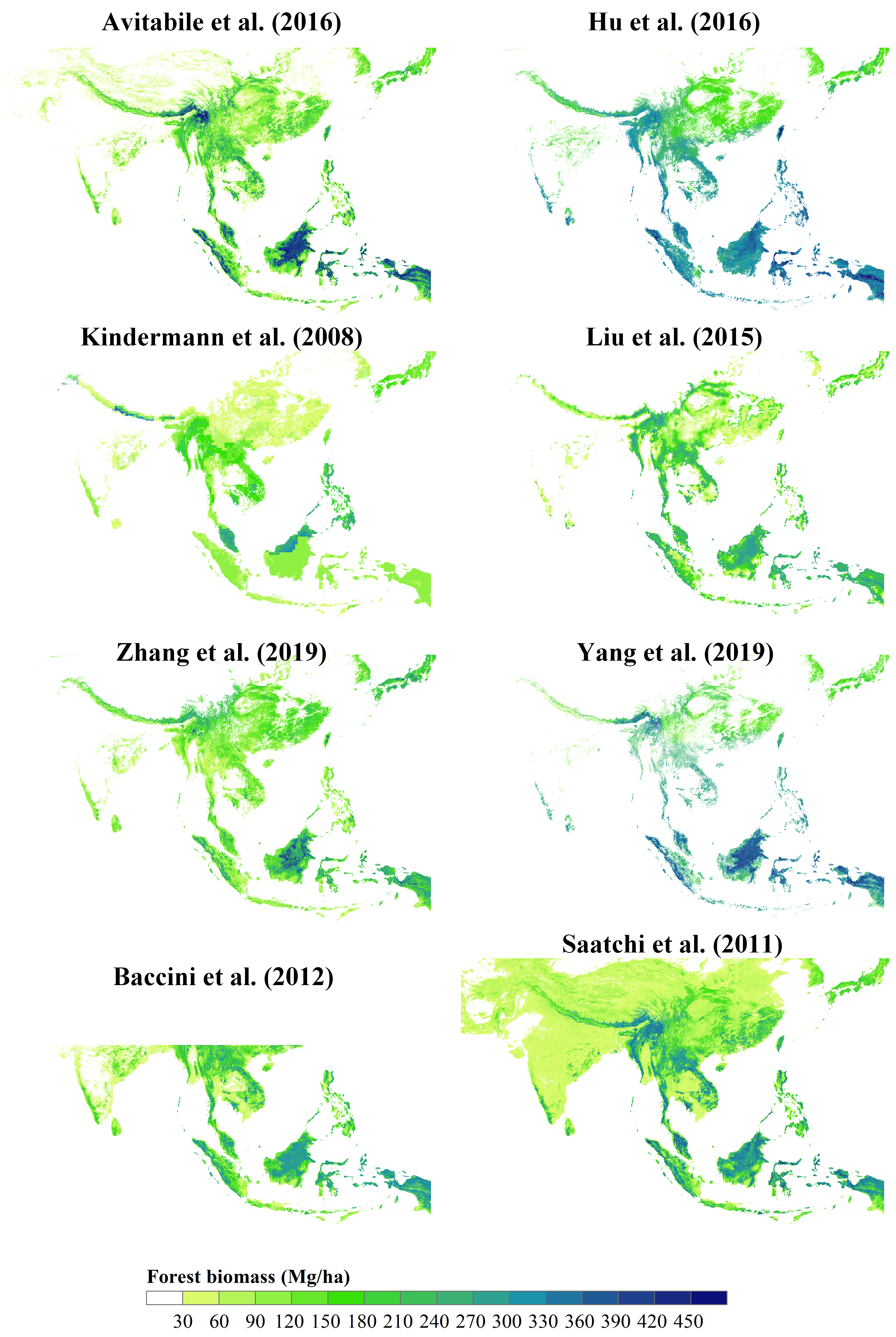
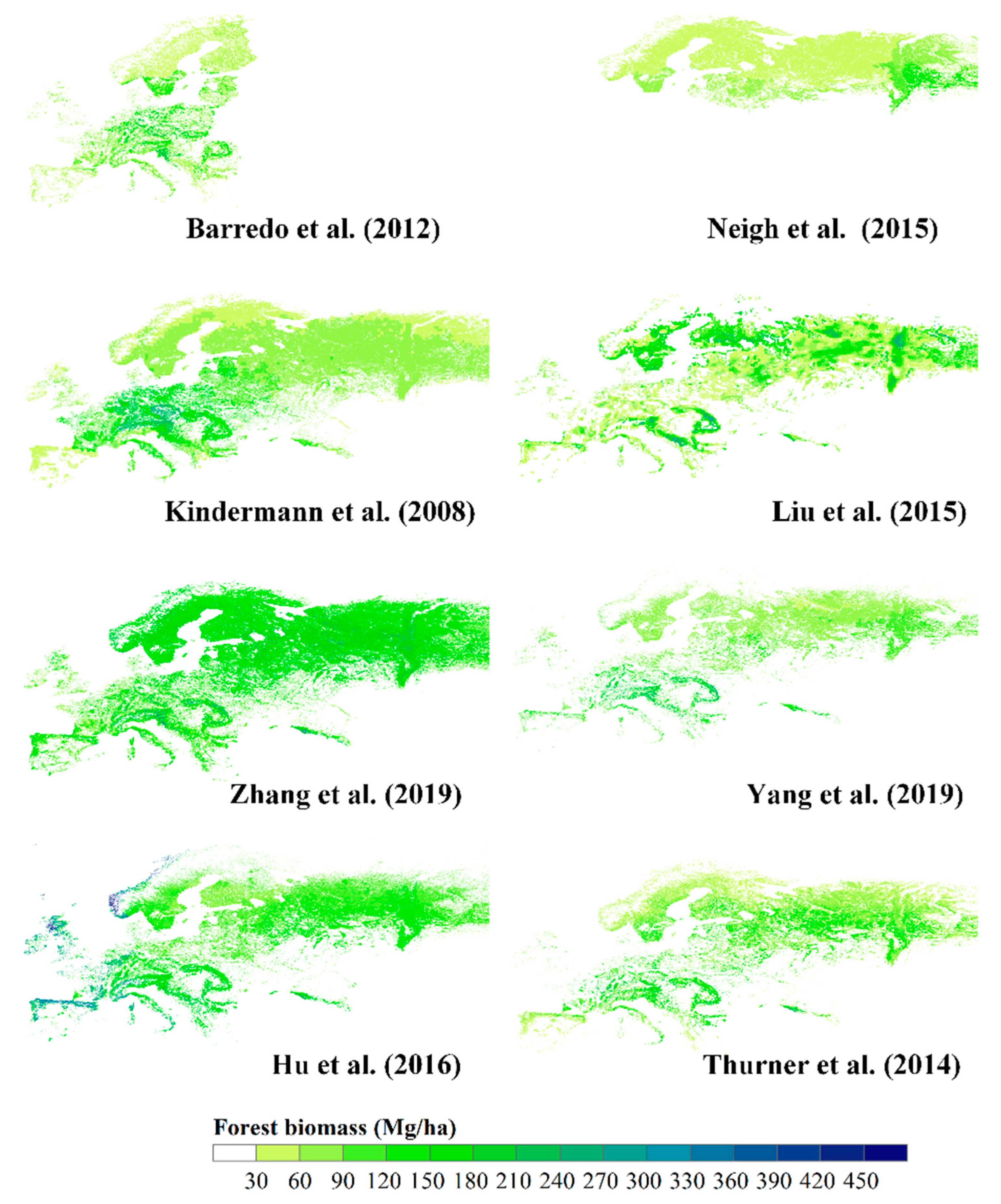
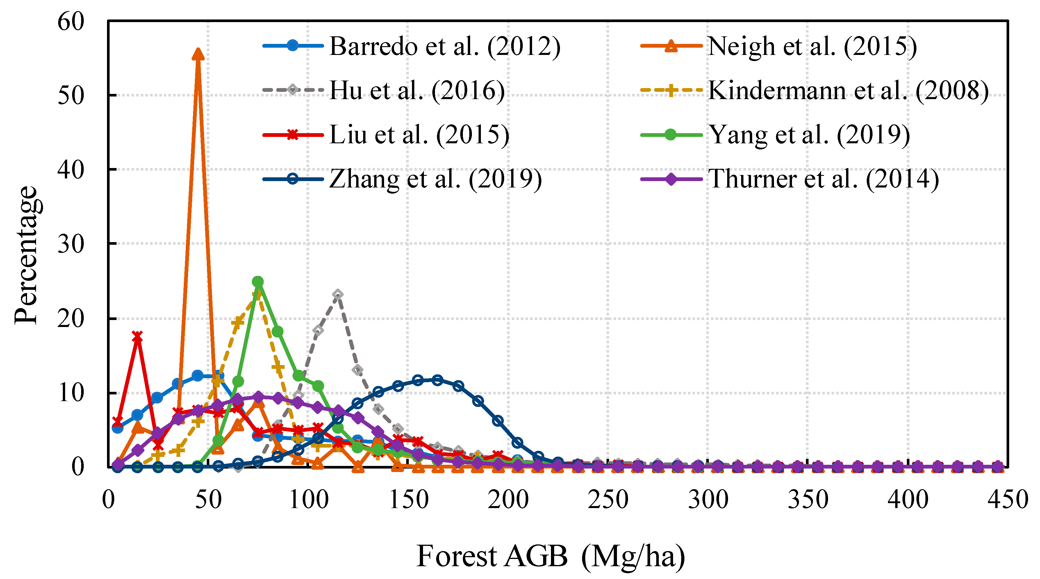
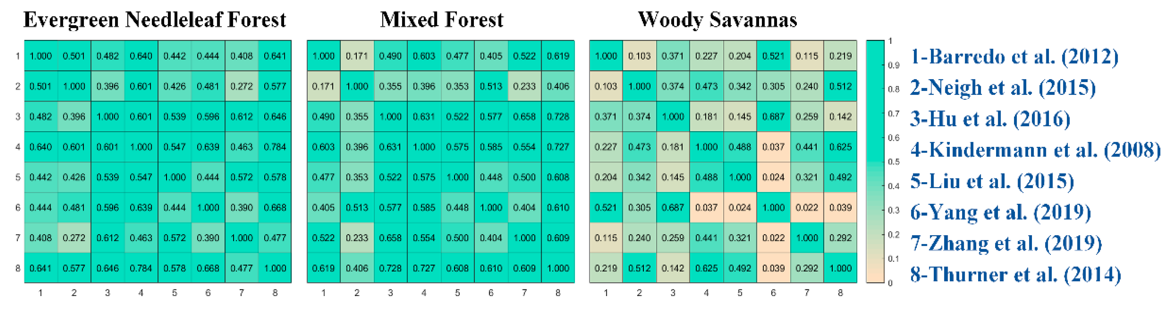
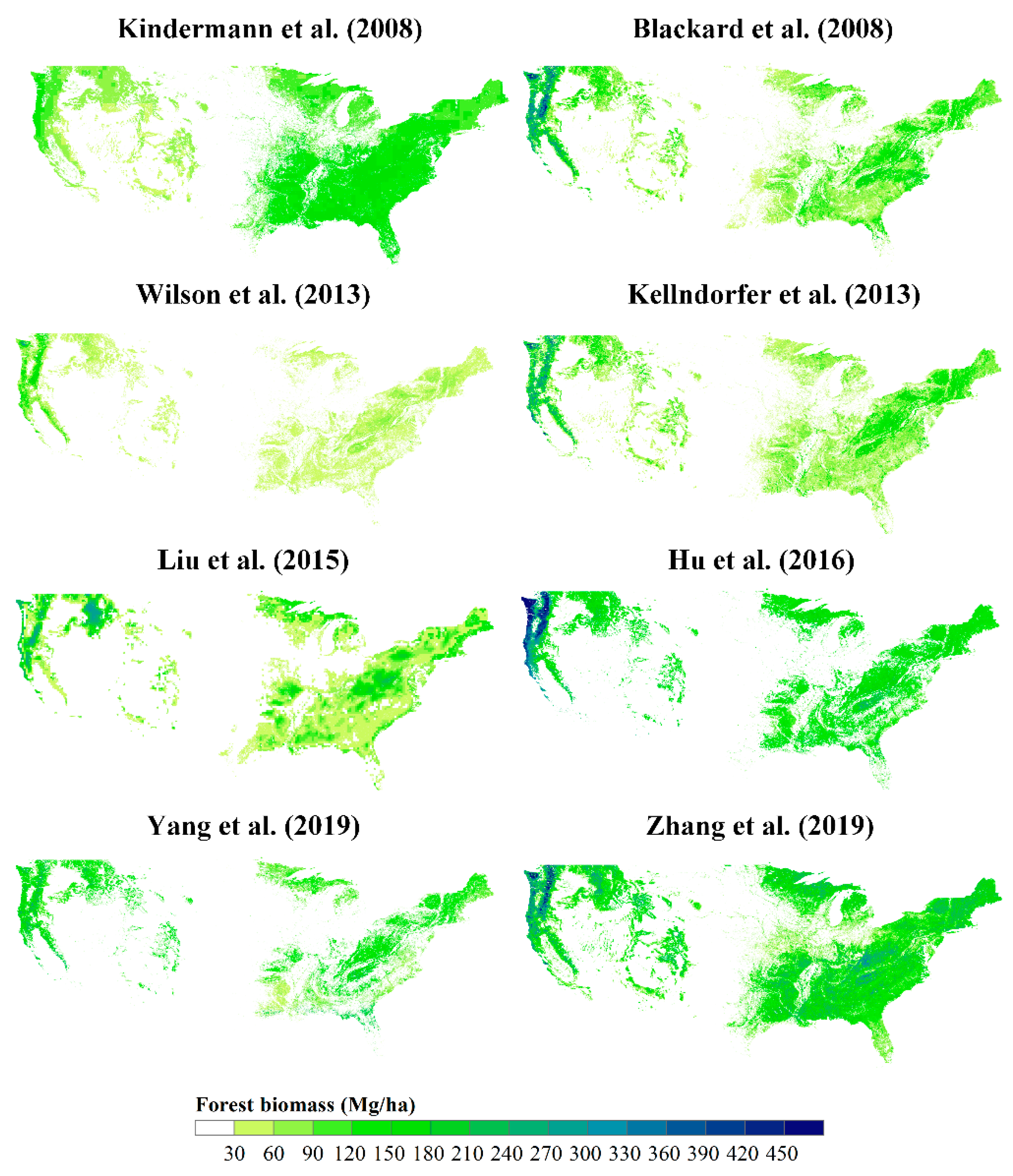
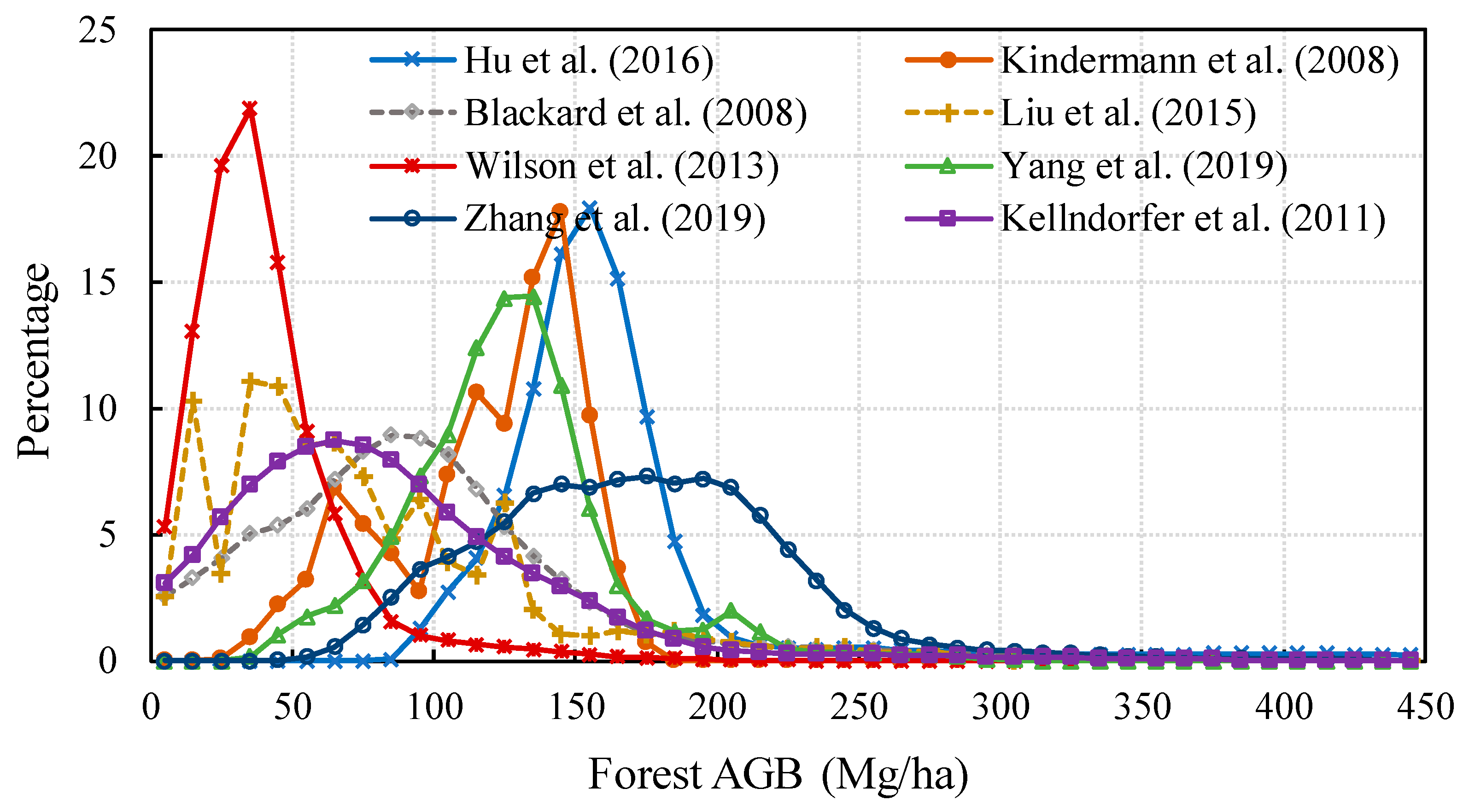
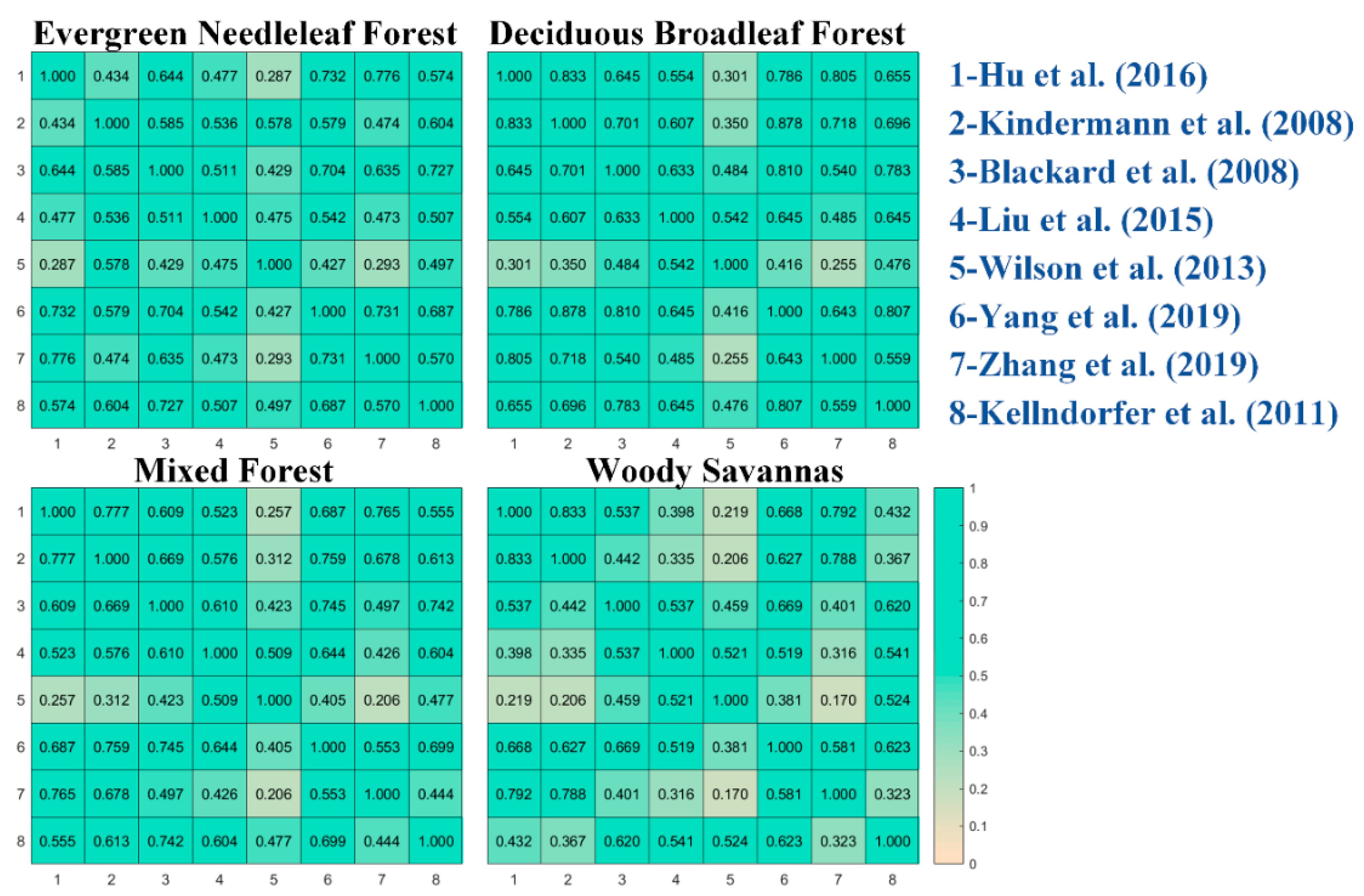
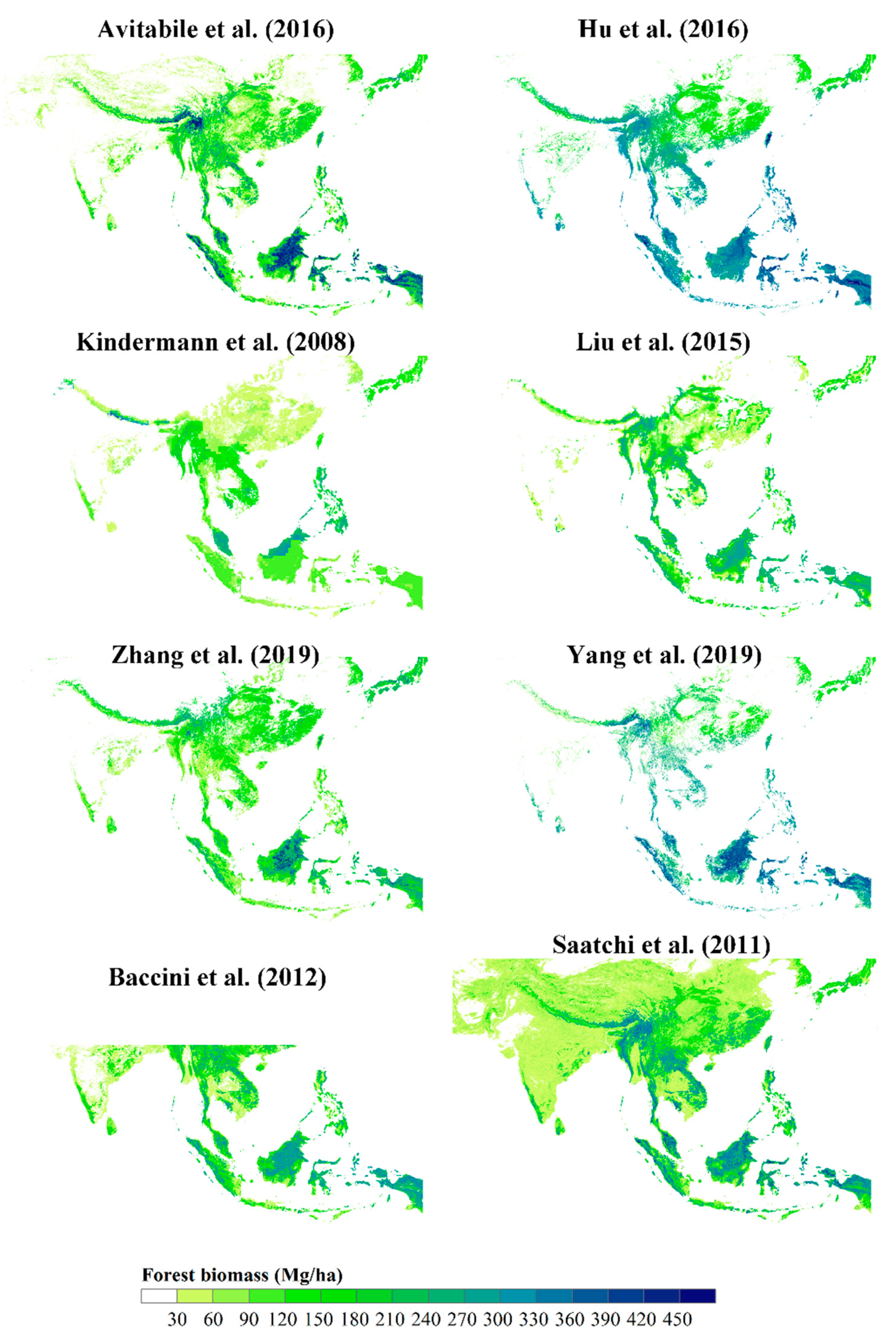
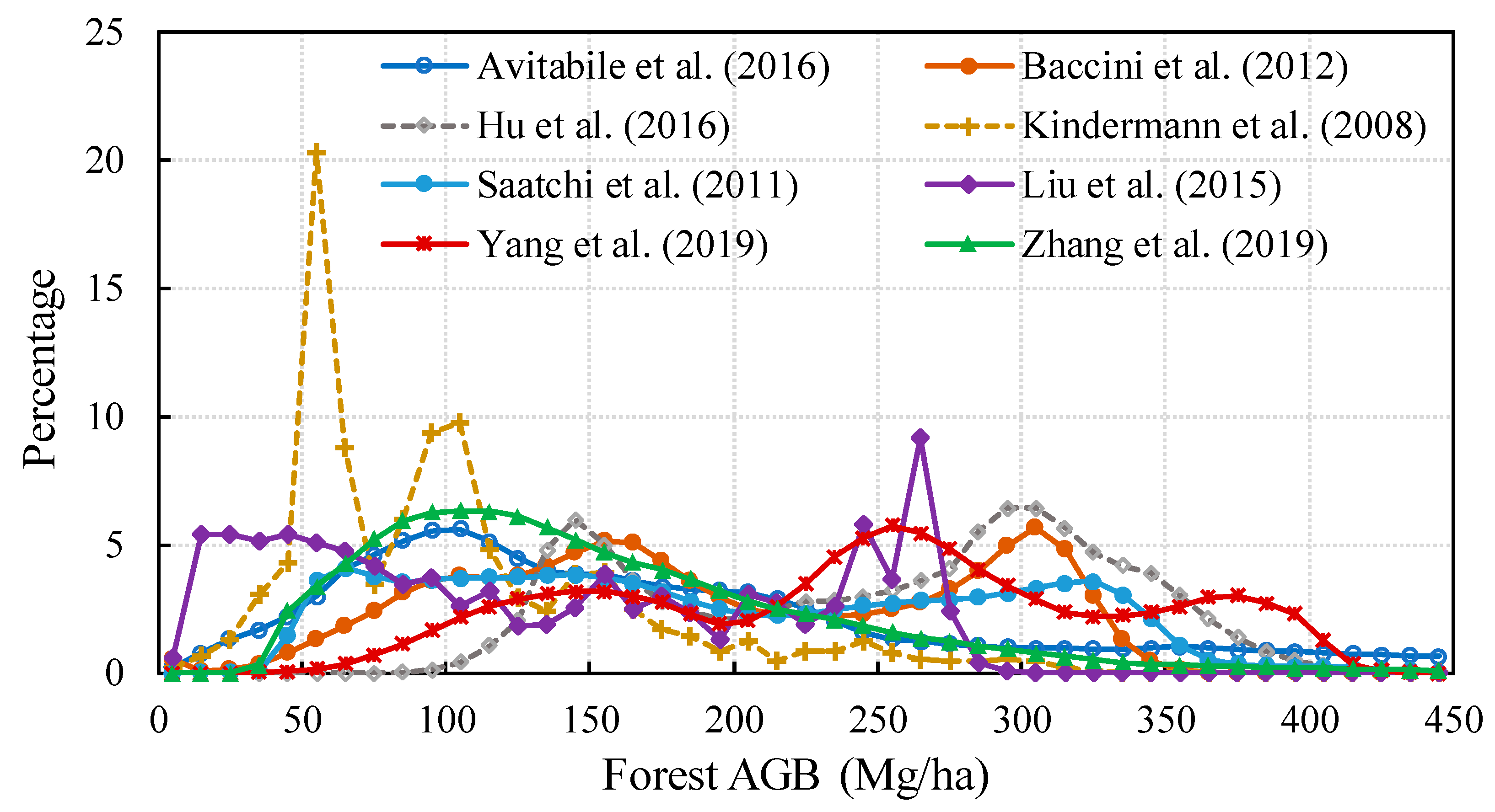
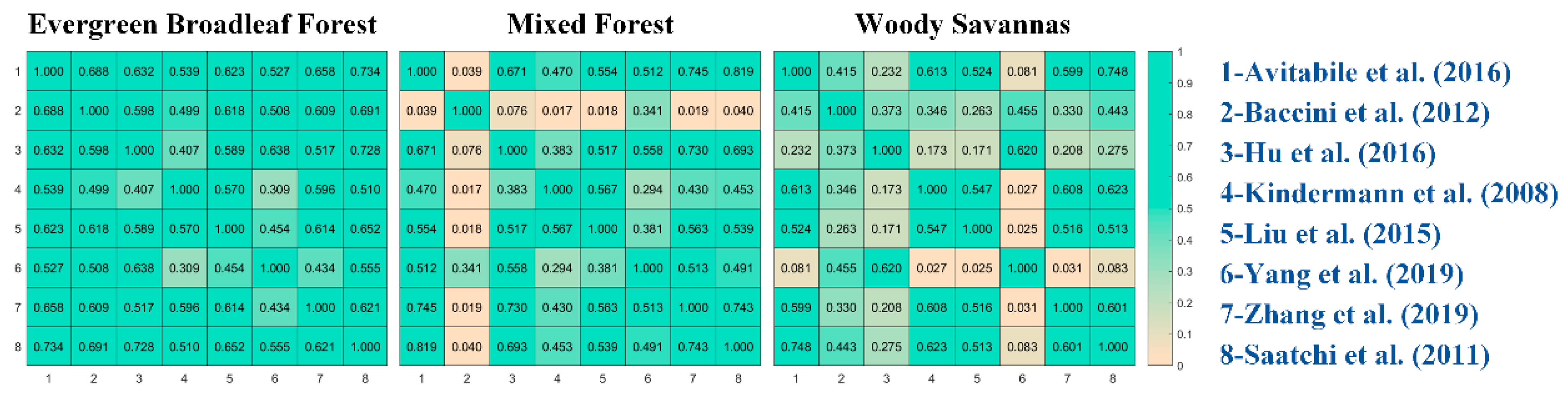
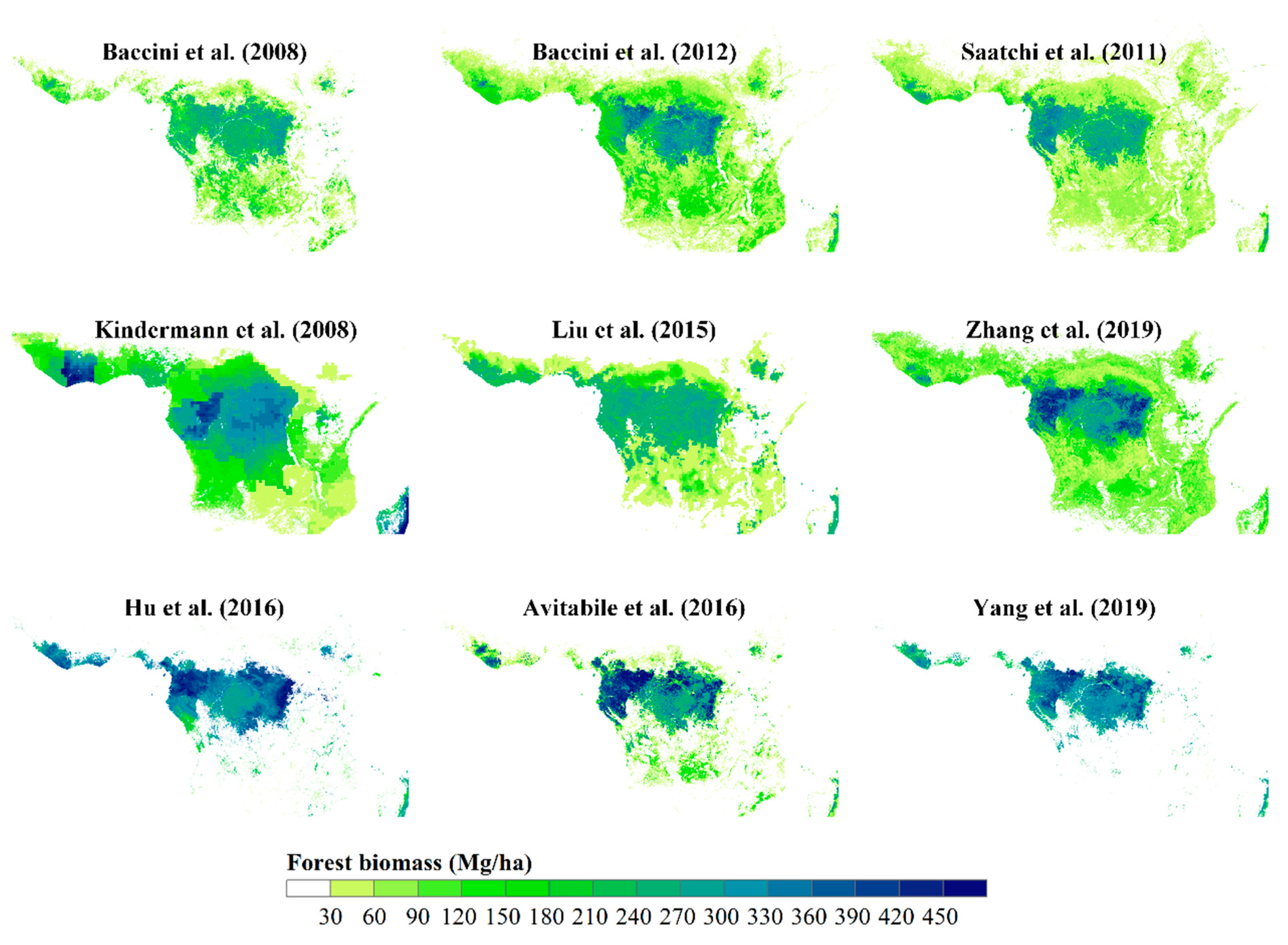
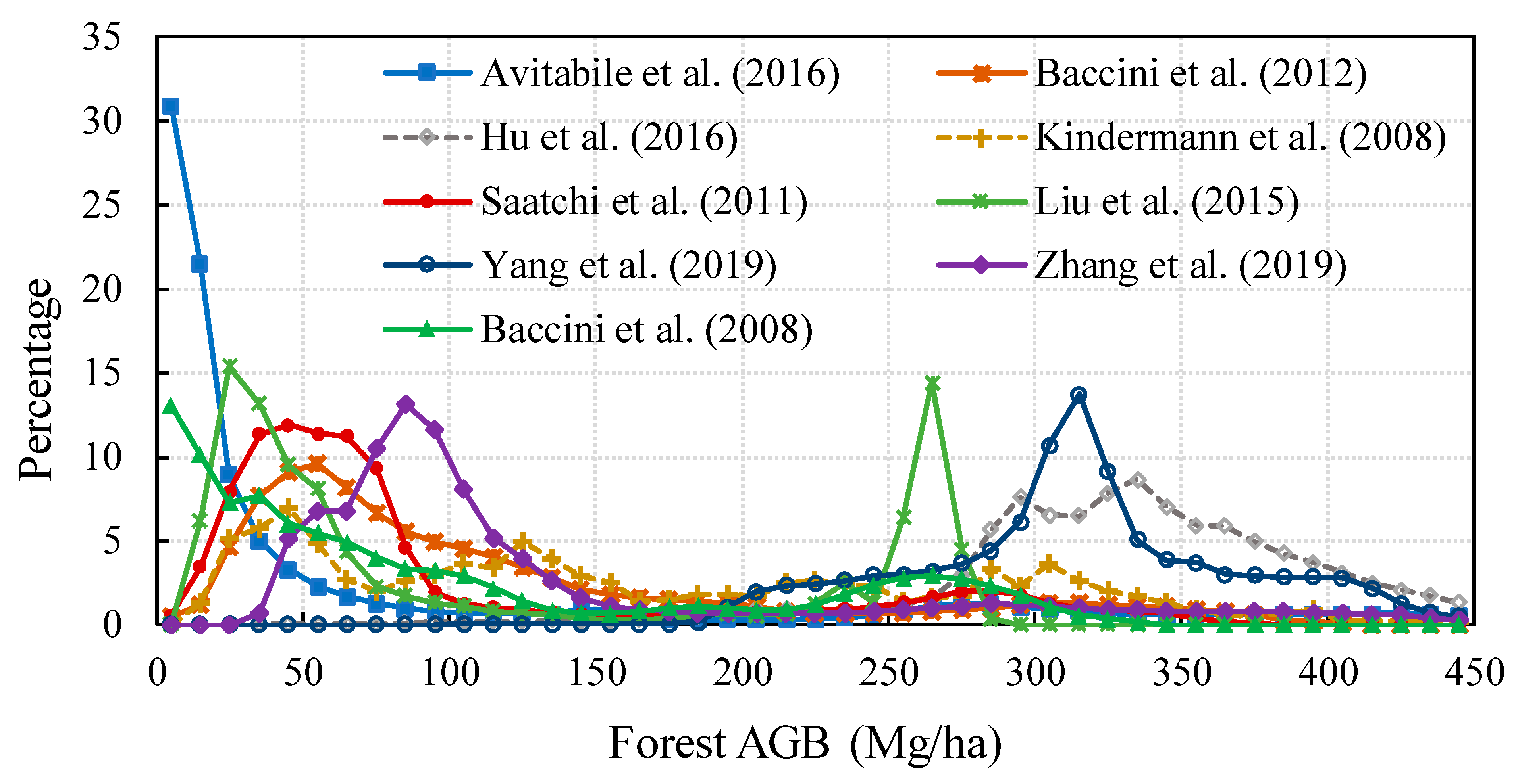
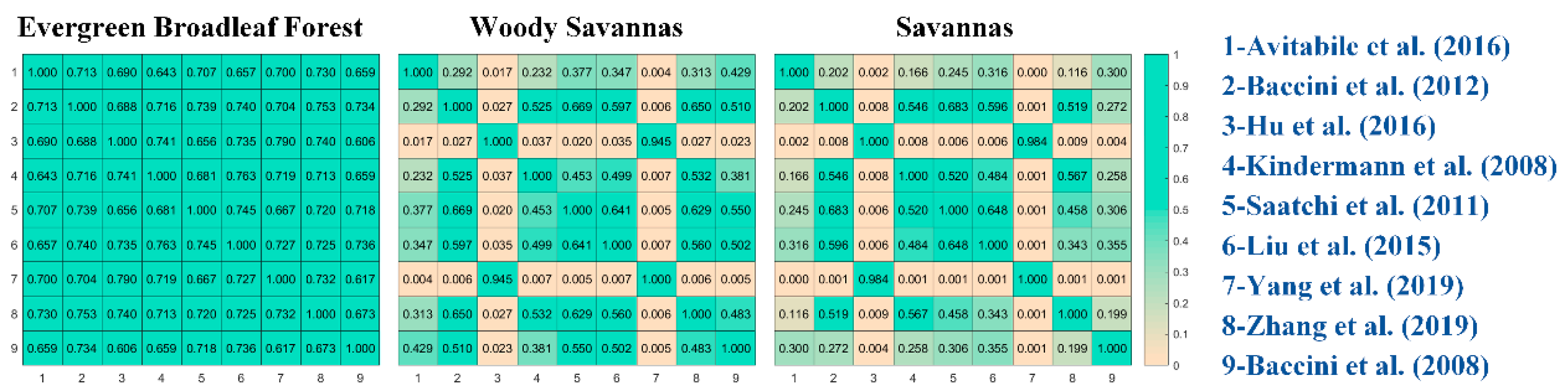
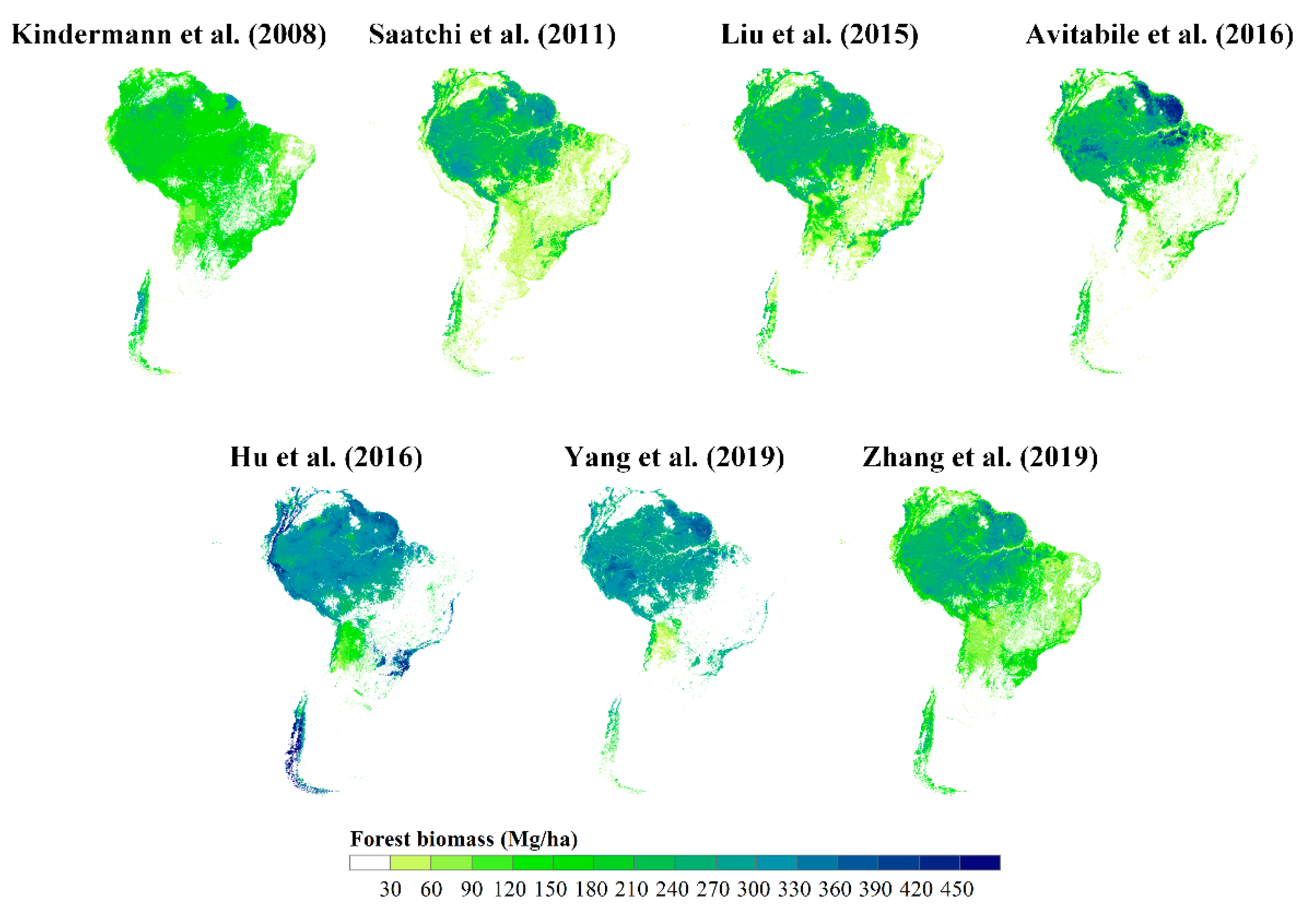
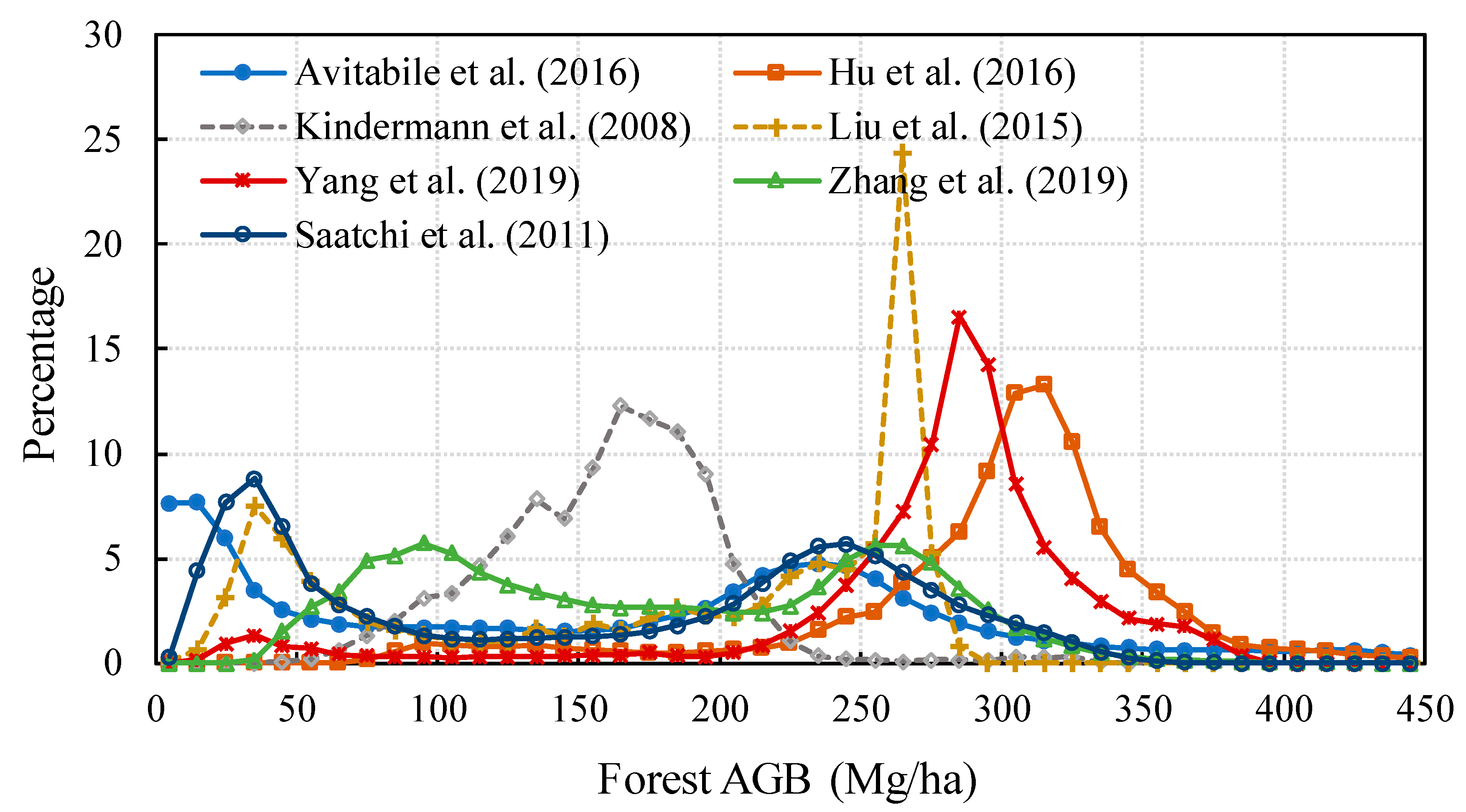
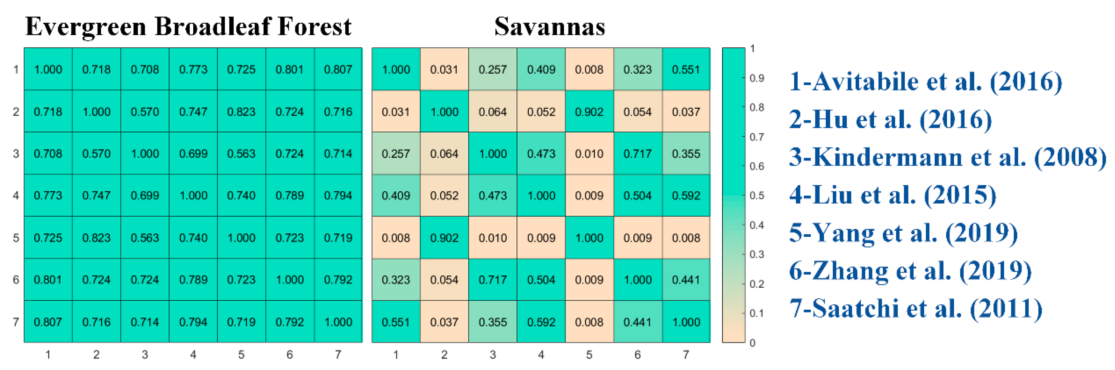
Table 1.
Summary of regional and global forest AGB maps.
| Region | Base Year | Pixel Size | Forest Mask | Methodology | Accuracy/Uncertainty | Provider |
|---|---|---|---|---|---|---|
| Global | 2000 | 1 km | GLC2000 | Stratify and multiply (IPCC defaults, GLC2000, ecoregion zones) | Not reported | Ruesch and Gibbs [49] |
| Global | 1950–2010, every 5 years | 1° | A compilation of land use maps | Interpolation (FAO, MCPFE, and UNECE) | Not evaluated formally | Hengeveld et al. [53] |
| Global | 2005 | 0.5° | GLC2000 | Downscaling (FRA biomass, NPP, human activity data) | Not reported | Kindermann et al. [54] |
| Global | 1993–2012 | 0.25° | MODIS IGBP land cover products | Regression (VOD data, Saatchi et al. map) | Not reported | Liu et al. [105] |
| Global | 2004 | 1 km | MODIS Land Cover Type (MCD12Q1) | Random forest model (field data, GLAS data, optical imagery, climate data, and topographic data) | R2 = 0.56; RMSE = 87.53 Mg/ha | Hu et al. [99] |
| Global | 2005 | 1 km | MODIS land cover products | Gradient Boosting Regression Tree method (field data, MODIS, GLASS products, SRTM, climate data) | R2 = 0.90; RMSE = 35.87 Mg/ha (Independent validation data were compiled from field data and LiDAR-derived gridded data) | Yang et al. [100] |
| Global | 2000 s | 0.01 | Hansen et al. 2013 forest cover map (10% tree cover) | Random Forest algorithm (reference AGB data, GLASS data products, climate and topographic data) | R2 = 0.70; RMSE = 46.91 Mg/ha | Zhang and Liang [77] |
| Northern Hemisphere | 2010 | 0.01° | GLC2000 | BIOMASAR algorithm (ASAR, field inventory data) | R2 = 0.70~0.90 at regional scales | Thurner et al. [102] |
| Pan-European | 2000–2010 | 1 km | Land Cover UMD classification MOD12Q1 | Model Tree Ensemble method (GPP, FLUXNET observations) | R2 = 0.92 at regional level | Busetto et al. [107] |
| Europe | 2010 | 1 km | CORINE Land Cover 2006 map | IPCC Tier 1 method (FRA data, CORINE Land Cover data) | Not validated at the pixel level | Barredo et al. [51] |
| Europe | 2000 | 500 m/10 km | CORINE Land Cover 2000 map | Downscaling method (NFI data, MODIS data, meteorological data, and land cover data) | R = 0.97; Mean absolute error = 25 m3/ha (for growing stock) | Gallaun et al. [70] |
| Russia | 2000 | 500 m | GLC2000 and MOD12Q1 | Random Forest model (field data and MODIS reflectance data) | R2 = 0.61 (variance explained) | Houghton et al. [71] |
| Eurasia | 2005–2006 | 500 m | MOD12Q1 | Two and three-phase modelling (field data, GLAS data, land cover, ecoregion, and topographic data) | R2 = 0.60; RMSE = 58.47 Mg/ha | Neigh et al. [85] |
| China | 2001–2013 | 1 km | Vegetation map of China | Model tree ensembles approach (field data, MODIS reflectance data, climate data and forest type map) | R2 = 0.46; RMSE = 22.7 Mg/ha | Yin et al. [72] |
| China | 2004–2008 | 5.5 km | MODIS Land Cover Type product MCD12C1 | Downscaling approach (field inventory statistics and MODIS data) | R2 = 0.761 | Du et al. [73] |
| China | 2000 | 1 km | Chinese land use map | Random forest model (field data, GLAS data, optical imagery, climate data, and topographic data) | R2 = 0.75; RMSE = 42.39 Mg/ha | Su et al. [98] |
| Northeast China | 2005 | 500 m | MODIS VCF (10% tree cover) | Random Forests model (field biomass data, GLAS data, and MODIS data) | R2 = 0.82; RMSE = 32.69 Mg/ha; Bootstrap uncertainty = 25.80 Mg/ha | Zhang et al. [97] |
| North America | 2005–2006 | 500 m | EOSD2000 and NLCD2001 | Three-phase modelling (field data, airborne LiDAR, GLAS data, and MODIS data) | Relative error = 1.9% | Margolis et al. [88] |
| Canada | 2001 and 2011 | 250 m | EOSD land cover data | kNN (NFI data, MODIS data, climate and topographic data, and land cover information) | R2 = 0.62; Relative root mean-squared deviation = 69.2; Relative mean deviation = 1.47 | Beaudoin et al. [68] |
| United States | 2000 | 30 m | NLCD 2001 | Regression tree modelling (FIA data, Landsat, NLCD land cover, and SRTM) | R = 0.7; RMSE = 139 Mg/hm2 | Kellndorfer et al. [59] |
| United States | 2001 | 250 m | NLCD92 | Classification and regression tree modelling (FIA data, MODIS data, land cover data, and ancillary information) | R = 0.31~0.92; Relative Error = 0.51~0.92 | Blackard et al. [44] |
| Conterminous U.S. | 2000–2009 | 250 m | NLCD tree canopy cover | Phenological Gradient Nearest Neighbor (FIA data, MODIS data, and ancillary geospatial data) | Described by agreement coefficient, Kolmorogov-Smirnov statistic, and the slope of the reduced major axis regression line | Wilson et al. [63] |
| Alaska | 2009–2010 | 30 m | NLCD 2001 | regression analysis (field AGB data and Landsat data) | Mean absolute error = 21.8 Mg/ha; Mean bias error = 5.2 Mg/ha | Ji et al. [64] |
| Garcia River Tract, Anne Arundel and Howard Counties, Parker Tract, and Hubbard Brook Experimental Forest | 2011 | 20–50 m | – | Several statistical models (field data and LiDAR data) | Represented by the 95% confidence interval | Cook et al. [78] |
| Maine | 2012 | 13 m | – | Space-varying coefficients model (field inventory data, and LiDAR data) | RMSE = 17.52 Mg/ha (prediction) | Babcock et al. [79] |
| Maryland | 2011 | 30 m | – | Random Forest regression model (field data, and LiDAR data) | Represented by the 95% confidence interval | Dubayah et al. [81] |
| Sonoma County | 2013 | 30 m | CALVEG land cover product | Random Forest regression model (field data, and LiDAR data) | Represented by the lower 10th percentile and upper 90th percentiles of confidence interval | Dubayah et al. [82] |
| Mexico | 2004–2007 | 30 m | INEGI land use map | Random Forest modelling (field inventory data, Landsat data, MODIS data, PALSAR data, and SRTM data) | R2 = 0.5; RMSE = 14 t C/ha (in the case of flat terrain) | Cartus, Kellndorfer, Walker, Franco, Bishop, Santos and Fuentes [65] |
| Mexico | 2008 | 250 m | INEGI land use map | MaxEnt (field inventory data, MODIS data, PALSAR data, and SRTM data) | R2 = 0.31; RMSE = 17.3 t C/ha | Rodríguez-Veiga et al. [66] |
| Tropical Africa and southeast Asia | 1980 and 2000 | 0.045° | GLC2000 | Rule-based GIS models (climate data, soil, topographic data, and land-use information, and population data) | Not reported | Gibbs and Brown [57,58] |
| Tropical regions | early 2000s | 1 km | MODIS VCF (10% tree cover) | MaxEnt (field measurements, GLAS data, optical and microwave imagery) | Uncertainty from±6% to ±53% | Saatchi et al. [19] |
| Pan-tropical regions | Circa 2007–2008 | 500 m | MODIS IGBP land cover type | Random Forest algorithm (field data, GLAS and MODIS data) | RMSE = 25 Mg C/ha for tropical America, 14 Mg C/ha for Africa, and 24 Mg C/ha for Asia | Baccini et al. [18] |
| Pan-tropical regions | 2000 | 30 m | Hansen et al. 2013 data and national tree cover loss/deforestation data | Random Forest model (field data, Landsat, GLAS, SRTM, and climate data) | Not reported | Baccini et al. [91] |
| Pan-tropical regions | 2000–2008 | 1 km | GLC2000 | Weighted linear averaging method (biomass reference datasets, Saatchi et al. 2011 biomass map and Baccini et al. 2012 biomass map) | RMSE = 87~98 Mg/ha; Mean error: almost null in most cases | Avitabile et al. [103] |
| Africa | 2000 | 1 km | GLC2000 | Regression tree model (field data, GLAS, and MODIS data) | R2 = 0.82; RMSE = 50.5 Mg/ha | Baccini et al. [89] |
| Amazon | 2005 | 40 m and 1 km | – | Combination (canopy height map and individual-based forest gap model) | R2 = 0.41; RMSE = 73 Mg/ha | Rödig et al. [106] |
| Amazon basin | 2000–2004 | 1 km | Vegetation map of the Amazon basin derived from remote sensing data | Decision tree approach (field data, MODIS, QSCAT, SRTM, JERS-1 and climate data) | More than 80% accuracy | Saatchi et al. [5] |
| Amazon basin | 2000–2004 | 5 km | – | MaxEnt (field data, MODIS, QSCAT, SRTM, climate data, and soil data) | Not reported | Saatchi et al. [74] |
| Brazil | Not for a specific period | 50 m | Up-to-date LULC map | Combination (exiting biomass maps, and LULC map) | R = 0.59 | Englund et al. [104] |
| Cambodia | 2009–2010 | 50 m | Land use/land cover map based on ASTER 2005 data | Multiple linear regression (field plots, PALSAR, and SRTM) | R2 = 0.61; RMSE = 21 Mg/ha | Avtar et al. [75] |
| Colombia | 2001–2006 | 500 m | IGAC forest map | Regression method (field data and MODIS data) | Not reported | Anaya et al. [76] |
| Panama | 2008–2012 | 1 ha | – | Random Forest algorithm (field plot data, GLAS, MODIS, SRTM data, and climate data) | Average pixel-level uncertainty = 20.5 Mg C/ha | Asner et al. [92] |
| Peru | 2012–2013 | 1 ha | – | Random Forest algorithm (field data, airborne LiDAR, MODIS, SRTM, and climate data) | R2 = 0.82; RMSE = 27.4 Mg C/ha (modelled relationship between top-of-canopy height and aboveground carbon density) | Asner et al. [93] |
| French Guiana | 2003–2012 | 1 km | Forest landscape type map | Regression Kriging technique (field data, GLAS, MODIS, PALSAR, geological map, forest landscape data, and climate data) | R2 = 0.48; RMSE ~= 51 Mg/ha | Fayad et al. [94] |
| Madagascar | 2010 | 250 m | The cloud-free year 2000 forest map obtained from Harper’s map and Hansen tree cover map | Random Forest regression (field biomass, MODIS, topography, and climate data) | R2 = 0.70; RMSE = 40 Mg/ha | Vieillendent et al. [95] |
© 2019 by the authors. Licensee MDPI, Basel, Switzerland. This article is an open access article distributed under the terms and conditions of the Creative Commons Attribution (CC BY) license (http://creativecommons.org/licenses/by/4.0/).
Share and Cite
MDPI and ACS Style
Zhang, Y.; Liang, S.; Yang, L. A Review of Regional and Global Gridded Forest Biomass Datasets. Remote Sens. 2019, 11, 2744. https://0-doi-org.brum.beds.ac.uk/10.3390/rs11232744
AMA Style
Zhang Y, Liang S, Yang L. A Review of Regional and Global Gridded Forest Biomass Datasets. Remote Sensing. 2019; 11(23):2744. https://0-doi-org.brum.beds.ac.uk/10.3390/rs11232744
Chicago/Turabian StyleZhang, Yuzhen, Shunlin Liang, and Lu Yang. 2019. "A Review of Regional and Global Gridded Forest Biomass Datasets" Remote Sensing 11, no. 23: 2744. https://0-doi-org.brum.beds.ac.uk/10.3390/rs11232744
Note that from the first issue of 2016, this journal uses article numbers instead of page numbers. See further details here.