Article

Mapping of Soil Total Nitrogen Content in the Middle Reaches of the Heihe River Basin in China Using Multi-Source Remote Sensing-Derived Variables

1
Department of Geography, Humboldt University of Berlin, Unter den Linden 6, 10099 Berlin, Germany
2
Department of Computational Landscape Ecology, Helmholtz Centre for Environmental Research–UFZ, Permoserstraße 15, 04318 Leipzig, Germany
3
College of Resources and Environmental Sciences, Nanjing Agricultural University, Weigang 1, Nanjing 210095, China
4
Jiangsu Academy of Agricultural Sciences, Zhongling Street 50, Nanjing 210014, China
*
Author to whom correspondence should be addressed.
Remote Sens. 2019, 11(24), 2934; https://0-doi-org.brum.beds.ac.uk/10.3390/rs11242934
Submission received: 3 November 2019 / Revised: 30 November 2019 / Accepted: 6 December 2019 / Published: 7 December 2019

Abstract

:
Soil total nitrogen (STN) is an important indicator of soil quality and plays a key role in global nitrogen cycling. Accurate prediction of STN content is essential for the sustainable use of soil resources. Synthetic aperture radar (SAR) provides a promising source of data for soil monitoring because of its all-weather, all-day monitoring, but it has rarely been used for STN mapping. In this study, we explored the potential of multi-temporal Sentinel-1 data to predict STN by evaluating and comparing the performance of boosted regression trees (BRTs), random forest (RF), and support vector machine (SVM) models in STN mapping in the middle reaches of the Heihe River Basin in northwestern China. Fifteen predictor variables were used to construct models, including land use/land cover, multi-source remote sensing-derived variables, and topographic and climatic variables. We evaluated the prediction accuracy of the models based on a cross-validation procedure. Results showed that tree-based models (RF and BRT) outperformed SVM. Compared to the model that only used optical data, the addition of multi-temporal Sentinel-1A data using the BRT method improved the root mean square error (RMSE) and the mean absolute error (MAE) by 17.2% and 17.4%, respectively. Furthermore, the combination of all predictor variables using the BRT model had the best predictive performance, explaining 57% of the variation in STN, with the highest R2 (0.57) value and the lowest RMSE (0.24) and MAE (0.18) values. Remote sensing variables were the most important environmental variables for STN mapping, with 59% and 50% relative importance in the RF and BRT models, respectively. Our results show the potential of using multi-temporal Sentinel-1 data to predict STN, broadening the data source for future digital soil mapping. In addition, we propose that the SVM, RF, and BRT models should be calibrated and evaluated to obtain the best results for STN content mapping in similar landscapes.

1. Introduction

As a major component of the terrestrial nitrogen (N) pool, soil total nitrogen (STN) not only provides essential nutrients for plant growth but also affects soil function and the concentration of greenhouse gases in the atmosphere. Low STN values limit plant growth while excessive STN may result in loss of nitrogen from the soil, causing soil fertility degradation and water pollution [1]. Soil degradation associated with soil nitrogen loss reduces soil security and greatly contributes to climate change. In total, 21% of the total annual emissions of nitric oxide (NO) are related to soil degassing [2]. On a global scale, NO emissions from soil and from fossil fuel combustion are in the same range [3,4]. In addition, as a key indicator of soil fertility and quality, STN content is closely related to agricultural productivity and food security. Therefore, reliable predictions of STN content are critical to sustaining sustainable agricultural development and understanding the regional N cycle. Up to date STN maps are important to identify spatial variation and control factors of STN, which can help maintain food security and soil security and provide a reference for managing climate change. To address environmental challenges, such as climate change and land degradation, an accurate and efficient method is needed to predict the spatial distribution of STN and improve its prediction accuracy.
Digital soil mapping provides a low-cost and efficient method for predicting the spatial distribution of soil nutrients. Most digital soil mapping methods are based on soil landscape models, which establish mathematical or statistical relationships between soil properties and related environmental variables [5,6]. Many digital soil mapping methods have been used to predict soil properties, including generalized linear model (GLM), random forest (RF), artificial neural networks (ANNs), boosted regression trees (BRTs), support vector machine (SVM), and regression kriging (RK). Although these models have achieved satisfactory results in different fields, choosing the best prediction method for a given landscape has always been a challenge. Jeong et al. [7] used RF and SVM models to conduct STN mapping studies in the Soyang lake watershed in South Korea and found that the RF model performed better while Were et al. [8] found that the latter performed better than the former in Kenya. Akpa et al. [9] reported that the RF model was superior to BRT in the prediction of soil properties in Nigeria while Yang et al. [10] found that the latter had better predictive performance in an alpine ecosystem. Because these studies obtained inconsistent results for different environments, the predictive models should be compared and evaluated for a given landscape.
STN prediction using digital soil mapping techniques requires sufficient environmental information. Commonly used environmental data are on land use/land cover (LULC), the climate, the topography, as well as remote sensing-derived variables. Remote sensing has received recent attention to improve digital soil mapping due to the extensive area it can cover and the rich spatial information it provides. Optical satellite imagery is one of the most commonly used remote sensing data sources for digital soil mapping and has contributed significantly to research on the prediction of STN. Recent studies have also noted the potential of synthetic aperture radar (SAR) for predicting soil chemical properties. For example, Bartsch et al. [11] explored the feasibility of C-band ENVISAT ASAR data in soil organic carbon (SOC) mapping and found that the SOC in the study area can be quantified by SAR images. Ceddia et al. [12] used optical and L-band ALOS PALSAR data to conduct SOC prediction studies in central Amazon, and found that the backscattering coefficient of SAR data can improve the prediction accuracy. A similar study was also reported by Ma et al. [13], who used SAR (Sentinel-1) and optical (Landsat 7) images to map soil properties in eastern China.
A wide range of information can be extracted from SAR data [14], the most common of which is the backscatter coefficient. The backscattering intensity of SAR data can be used to obtain information about surface properties and has been widely used in soil science research to obtain information about soil roughness [15], soil moisture [16], and soil salinity [17]. The application of SAR images in mapping soil properties depends on the sensitivity of backscattering intensity to changes in soil moisture and land surface conditions [18]. Yang et al. [19] found a significant correlation between SAR backscatters and various soil properties (including SOC, STN, and sand) during the growing season, and reported that multi-temporal SAR data is useful for predicting soil chemical properties because it can capture soil–vegetation relationships. Similar results have been reported by, for example, Maynard et al. [20] and Takada et al. [21]. The soil–vegetation relationships observed in these studies can explain the spatial variation of the soil and thus help remote sensing techniques to predict soil properties [22,23]. Although SAR data is a promising data source for digital soil mapping, few studies have used the backscatter coefficients of SAR data as predictor variables for STN mapping.
Arid and semi-arid areas account for about 50% of China’s land surface. Due to irrational land use of these areas, as well as a decline in soil fertility and a lack of water resources, desertification in such areas is intensifying. Hence, greater attention should be given to the variation in soil properties here. Representing both arid and semi-arid regions in China, the spatial distribution of soil properties in the Heihe River Basin (HRB) has attracted the attention of researchers in recent years. However, these studies have focused primarily on SOC [24,25] and soil texture [26], with little information on STN in the area. This study used machine learning algorithms to predict the STN content in the middle reaches of the HRB in Northwest China. The specific objectives were (i) to explore whether adding SAR data improves STN prediction; (ii) to evaluate and compare the performance of RF, BRT, and SVM models; and (iii) to assess the importance of predictor variables in mapping the STN content of the study area. For these purposes, 15 predictor variables (including the climate, the topography, LULC, and remote sensing-derived variables) and 85 soil samples were obtained. The remote sensing images used in this study included optical (Landsat-8) and multi-temporal SAR (Sentinel-1A) data.

2. Materials and Methods
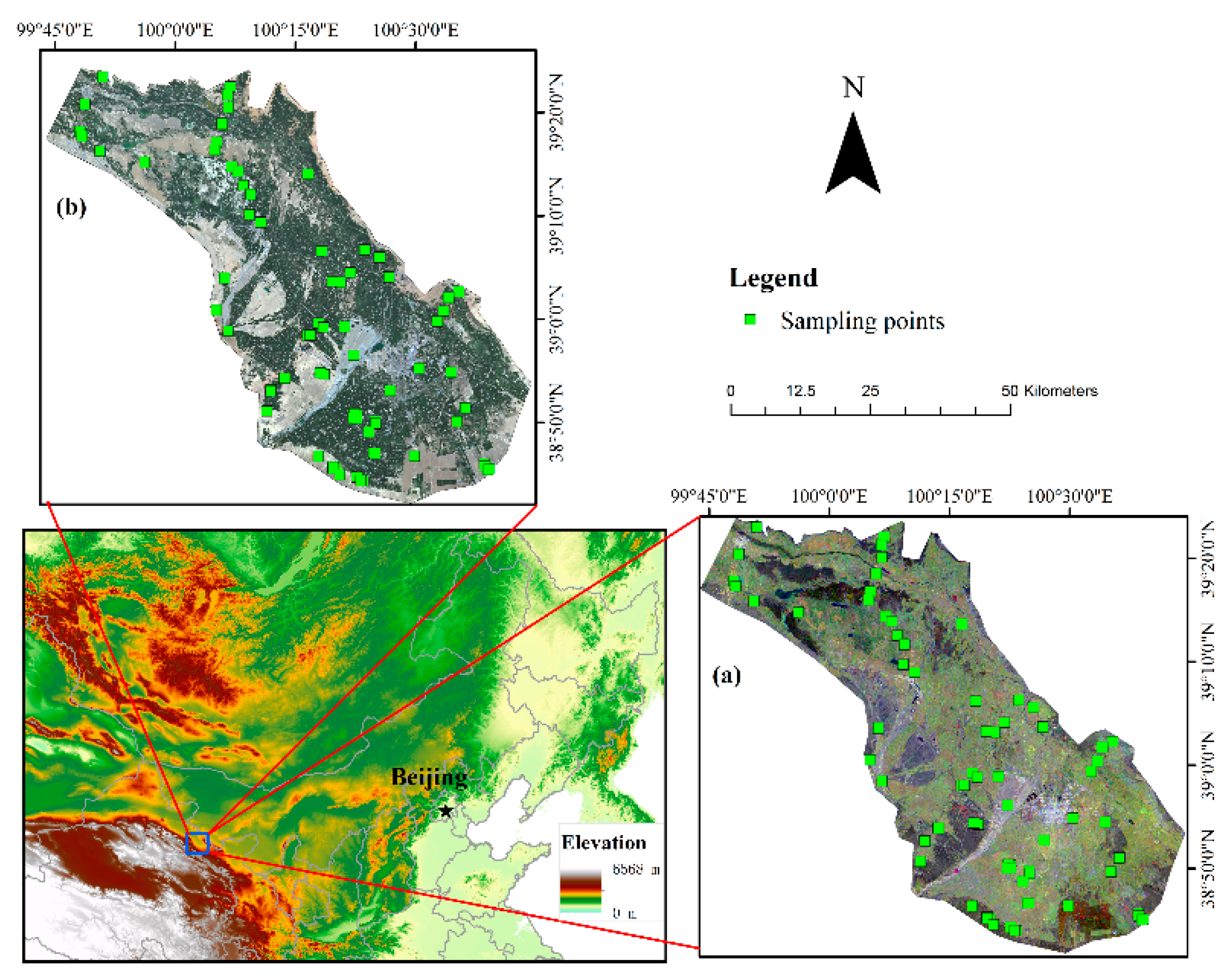
2.1. Study Area

The study area is in the middle reaches of the HRB (100.23° E, 39.06° N), which is located in Zhangye City, Gansu Province, in northwestern China (see Figure 1). HRB is China’s second largest inland river, covering an area of about 1.3 × 10⁵ km2 [27], with a total population in the middle reaches of 82.55 × 10⁴ in 2010 [28]. The study area exhibits a continental dry temperate climate, with a mean annual temperature (MAT) of approximately 6 to 8 °C and a mean annual precipitation (MAP) of 150 mm [29]. The elevation of the area is between 1300 and 1700 m above sea level. Major land use types are cultivated land, grassland, and barren land, and the main crops include corn and spring wheat. Precipitation in the middle reaches of the HRB is limited, with farmland accounting for about 86.85% of water consumption in the basin [30]. Gray-brown desert soil and gray desert soil are the zonal soil types in the study area [31].

2.2. Soil Data

A total of 85 soil samples (0–20 cm) were used to calibrate and validate the models (Figure 1), which were collected and provided by “Cold and Arid Regions Science Data Center at Lanzhou (CARD)”. Large-scale field sampling is time-consuming and labor-intensive. In order to obtain sufficient soil data to characterize the variation of soil properties, the purposive sampling strategy of Zhu et al. [32] was adopted. Soil sample sites were selected based on major soil formation factors, including topographical conditions, the climate, and LULC. Soil sampling was carried out from 2011 to 2014, and a 1-m deep soil pit was dug at each location. Coordinate information for each sample point was collected using a handheld global positioning system receiver, and environmental characteristics (including land use, vegetation, and elevation, etc.) were recorded. The samples were air dried, ground, and sieved at 2 mm, after which the STN content was determined using the Kjeldahl method.

2.3. Environmental Variables

The environmental variables used in this study for STN mapping included LULC, remote sensing-derived variables, and topographic and climate variables. These environmental data were collected from various sources and used to generate a total of 15 predictor variables. ArcGIS 10.2 was used to convert all environment variables to raster formats with the same 30-m resolution. These predictor variables and observed STN data were then imported into a geographic information system in a common coordinate reference system for future STN mapping. The pixel values of the predictor variables corresponding to each soil sample point based on these raster layers were calculated to build the models.

2.3.1. Remote Sensing Variables

The remote sensing images used in this study included SAR and optical data. The SAR image used in this study was Sentinel-1A that was downloaded from the ESA (European Space Agency), whereas the optical data was Landsat-8 OLI that was downloaded from the USGS (US Geological Survey). Designed by the ESA, Sentinel-1 is composed of two satellite constellations, including Sentinel-1A and Sentinel-1B [33]. The Sentinel-1A carries a C-band SAR imaging instrument that provides four imaging modes. In this study, 4 Sentinel-1A images (single-look complex (SLC) products) in the IW (interferometric wide swath) mode were obtained. More detailed information of the SAR data used in this study is provided in Table 1. We preprocessed these SAR data with SARscape 5.2, including multi-look, coregistration, speckle filtering (a 5 × 5 window Lee filter [34]), geocoding, and radiometric calibration [14]. These images were geocoded using the ASTER GDEM and their digital numbers (DN) were converted to decibel (dB) scale backscatter coefficients. Landsat-8 OLI images with cloud cover <10% from July to September 2015 were obtained; to represent vegetation intensity and type [6,10], the normalized difference vegetation index (NDVI) was calculated using bands 4 and 5. The relief correction of all images was performed based on the polynomial geometric correction method.
Because Landsat-8 OLI’s red band 4 (B4)—(0.64–0.67 μm), near-infrared band 5 (B5)—(0.85–0.88 μm), and shortwave infrared band 6 (B6)—(1.57–1.65 μm) represent vegetation growth, coverage and biomass [35], respectively, the three bands of Landsat-8 OLI were extracted as predictor variables to map STN. A total of eight environmental covariates were extracted from remote sensing images, four of which were from optical images and the remainder from SAR data.

2.3.2. Climate Variables

The MAP and MAT data for the study area from 1961 to 2010 were obtained from CARD (http://card.westgis.ac.cn/). We calculated the average MAP and MAT for 50 years (1961–2010) as predictor variables. These data were interpolated (high accuracy surface modeling (HASM) method [36]) from the measured values of 34 meteorological stations, 21 of which are conventional meteorological stations in the HRB and its surrounding areas, whereas the remainder are national reference stations around the Heihe River. The HASM method has been reported to improve the interpolation of climate variables compared to other conventional techniques [37].

2.3.3. Land Use/Land Cover Data

The LULC data were generated using Landsat TM and ETM remote sensing data from 2011 combined with field surveys and validation. The data were provided by CARD, classified into the following types of LULC: Farmland, grassland, barren, wetlands, forests, and villages.

2.3.4. Topographic Variables

A total of four topographic variables were calculated from the 30-m resolution ASTER GDEM (including elevation, slope, aspect, and topographic wetness index (TWI)) using SAGA GIS and ArcGIS 10.2. SAGA TWI was reported to predict more realistic soil wetness than the traditional TWI [10]. In this study, TWI was obtained using SAGA GIS and the remaining topographic variables were generated by ArcGIS 10.2.

2.4. Prediction Models

We applied three machine learning algorithms (i.e., RF, BRT, and SVM models) to predict STN. These models have a strong ability to model complex nonlinear relationships between soil properties and environmental variables. We optimized the parameters in these models through the grid search approach using the ‘caret’ package in the R software.
First introduced by Vapnik et al. [38], the SVM model originated from statistical learning theory and was applied to classification or regression. Based on the kernel function, the SVM model projects the input data onto the new hyperspace, optimally dividing all the data into different classes [39]. The four commonly used kernel functions are as follows: Linear, sigmoid, polynomial, and radial basis function (RBF). The selection of kernel functions can affect the prediction accuracy of the SVM model. The RBF kernel performs best at capturing nonparametric features [40] and has been successfully applied to soil mapping studies [5]. In this study, RBF was selected as the kernel model of the SVM model.
As a nonparametric method, the RF model is an ensemble machine learning algorithm used to perform classification and regression. During model training, the RF model generates a large number of random trees that are combined into a single prediction [41]. A unique bootstrap sample from the original training data was used to build each tree in the forest [42]. The samples in the RF method are divided into “in-bag” samples and “out-of-bag (OOB)” samples, and the latter are used to estimate errors [43].
Developed by Elith et al. [44], the BRT model is a machine learning technique that combines the advantages of boosting and regression trees. The regression tree is a model based on a decision tree that analyzes the variation of the response variables of a set of predictor variables [45]. As a machine learning technique similar to model averaging [46], boosting is a forward and stage-wise procedure that uses an iterative approach to develop the final model, gradually adding the tree to the model [47]. The BRT model relies on a stochastic gradient boosting procedure to improve model prediction accuracy and prevent data overfitting [48].

2.5. Statistical Analyses

This study used SPSS 24.0 software to perform a descriptive statistical analysis of STN and environmental variables to summarize these data. The following packages were used in the R software for STN mapping: ‘gbm’-package (BRT), ‘randomForest’-package (RF) and ‘kernlab’-package (SVM), and ‘raster’-package and ‘maptools’-package.

2.6. Model Validation

To explore the effectiveness and potential contribution of the backscatter coefficient of multi-temporal Sentinel-1 images to STN mapping, different combinations of environmental variables were constructed (Table 2). We then compared the predictive performance of different combinations based on RF, BRT, and SVM methods. To compare and evaluate the prediction accuracy of these models, a 10-fold cross-validation technique was used to calculate the following three commonly used validation indices: The root mean square error (RMSE), mean absolute error (MAE), and coefficient of determination (R2). These validation indices were defined as shown in Equations (1)–(3):
M A E = 1 n i = 1 n |   P i O i |
R M S E = 1 n i = 1 n ( P i O i ) 2
R 2 = i = 1 n ( P i O i ¯ ) 2 i = 1 n ( O i O i ¯ ) 2
where n represents the number of sample points; and Pi and Oi represent the estimated and observed STN content at site i, respectively.

3. Results

3.1. Descriptive Statistics

The statistical results of the STN content and the values of the predictor variables corresponding to the samples are shown in Table 3. The STN content in the topsoil ranged from 0.06 to 1.68 g kg−1 (the mean and median were 0.87 and 0.96 g kg−1, respectively), with a standard deviation (SD) of 0.34 g kg−1. The SD value of the STN content was lower than the mean value, indicating a moderate variation in its distribution [49]. The STN content (with a skewness coefficient of 0.33) had a slightly skewed distribution.

3.2. Model Performance

We constructed five STN content models based on different combinations of environmental variables: Model A represents environmental variables without SAR data while Model E was a combination of all environmental variables; Models B and C represent optical and SAR remote sensing variables, respectively; and Model D included variables derived from Landsat-8 and Sentinel-1 images. Table 4 shows the model performance statistics for the BRT, RF, and SVM techniques using these STN models. The BRT model obtained the highest accuracy to predict STN, with the highest R2 (0.57) value and the lowest RMSE (0.24) and MAE (0.18) values. The predictive performance of the BRT and RF models was significantly better than the SVM model. However, the prediction accuracy of the BRT model was closely followed by the RF model (R2 = 0.55, RMSE = 0.24, and MAE = 0.19).
Overall, for the RF, BRT, and SVM methods, Model C (combination of backscatter coefficients from multi-temporal SAR data) had a higher prediction accuracy than Model B (single-day Landsat-8-derived variables). This result indicates that SAR data not only provides important information for STN mapping but can also be as effective as optical images. Moreover, the predictive power of multi-temporal Sentinel-1A data was not inferior to the single-day Landsat-8 OLI image. Therefore, SAR data has broad application prospects in digital soil mapping, especially in those areas that are susceptible to cloud. For the three C models, the RF technique obtained the highest R2 (0.44) and the lowest RMSE (0.27) and MAE (0.22). The R2 value indicated that Model C, which was constructed using multi-temporal Sentinel-1A images, explained approximately 44% of the STN variation.
Using three different machine learning techniques, STN prediction accuracy was improved when multi-temporal Sentinel-1A images were combined with Landsat-8 images. The addition of SAR data using the BRT method resulted in 48.6%, 17.2%, and 17.4% improvements for R2, RMSE, and MAE, respectively. Improvements in the prediction accuracy of the STN were also observed when multi-temporal SAR data were added to Model A. For example, the addition of multi-temporal Sentinel-1A images using the BRT and RF models increased R2 from 0.52 to 0.57 and 0.52 to 0.55, respectively. The combination of all environmental variables (Model E) obtained the highest prediction accuracy compared to the other four models (Models A, B, C, and D), with R2 values of 0.57 and 0.55 for the BRT and RF modeling techniques, respectively. The R2 values indicated that the RF and BRT modeling techniques can explain 55% and 57% of the STN variation, respectively.

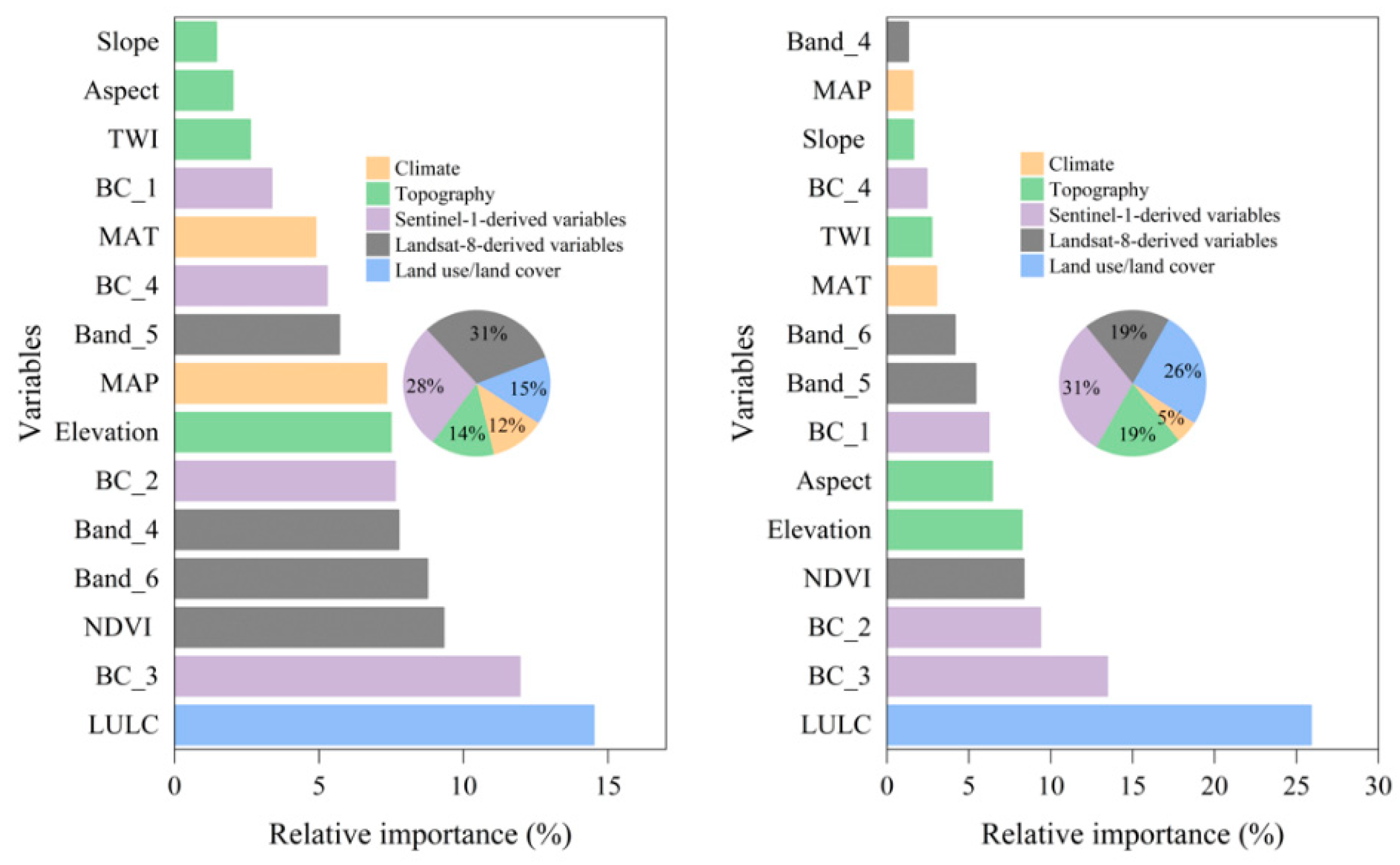
3.3. Relative Importance of Environmental Data

The relative importance of each predictor variable calculated using Model E in the RF and BRT modeling techniques is shown in Figure 2. In this study, the relative importance of predictor variables was normalized to 100% to facilitate comparisons among predictor variables. The relative importance of the same environmental variables in the RF and BRT models was slightly different. The five most important predictor variables for the RF model were LULC, BC_3, NDVI, Band_6, and Band_4 while in the BRT model, they were LULC, BC_3, BC_2, NDVI, and elevation. In both models, LULC and BC_3 had the same relative importance rankings, namely, first and second, respectively. These findings indicate that these environmental variables are the dominant predictor variables of STN mapping in this study area. In the RF model, Landsat-8-derived variables had the highest relative importance (with a relative importance of 31%), followed by Sentinel-1-derived variables (28%), LULC (15%), topographic (14%), and climate (12%) variables. The relative importance of Sentinel-1-derived variables, LULC, Landsat-8-derived variables, and topographic and climate variables in the BRT model were 31%, 26%, 19%, 19%, and 5%, respectively. Moreover, the remote sensing variables in the RF and BRT models had a relative importance of 59% and 50%, respectively.

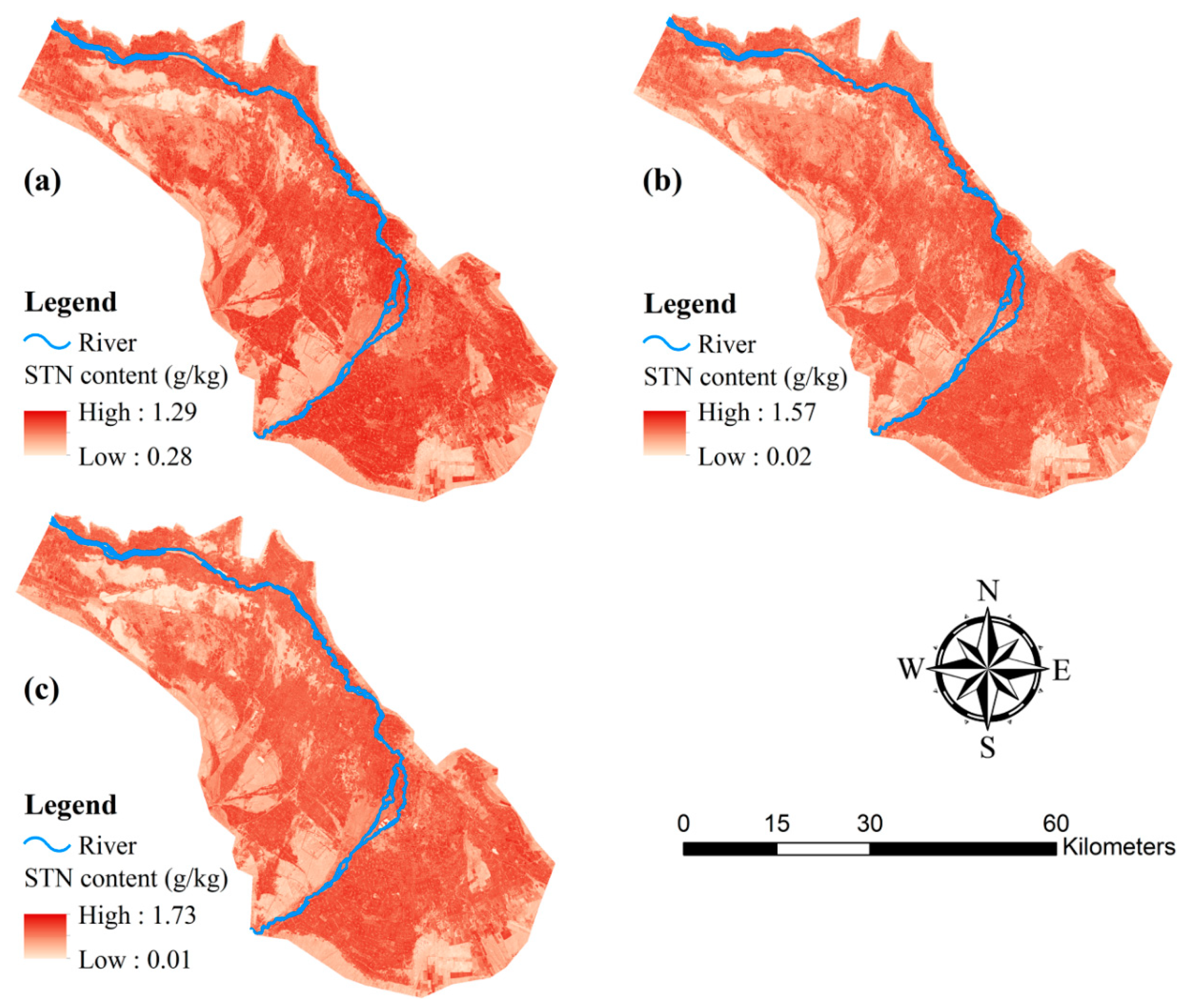
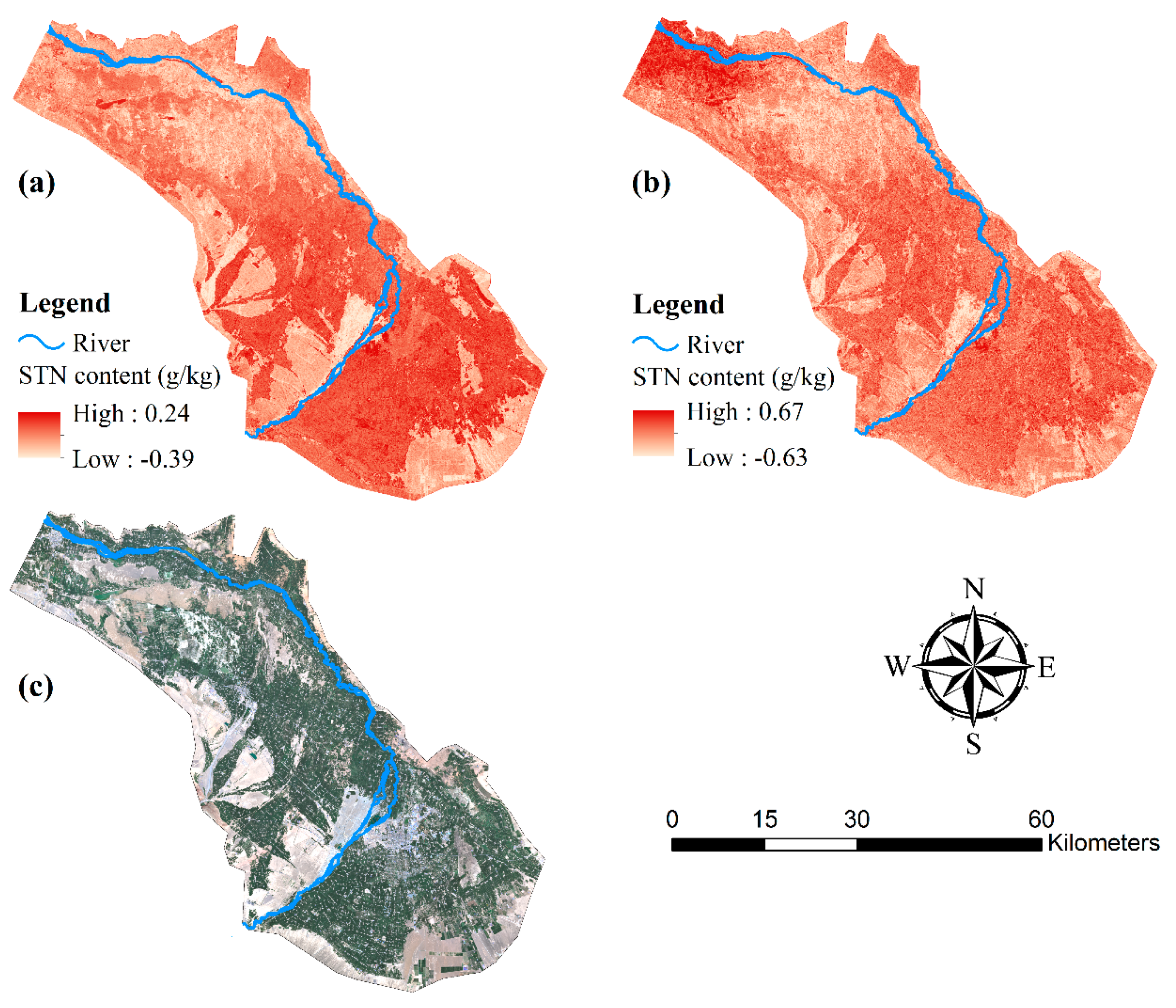
3.4. Spatial Prediction of STN Content

The spatial distribution maps and corresponding descriptive statistics of STN content predicted by the RF, BRT, and SVM methods using Model E are shown in Figure 3 and Table 5, respectively. Figure 4 shows STN maps predicted using Model D constructed by using only remote sensing variables. The mean (±SD) values of the STN content predicted by the RF, BRT, and SVM methods were 0.81 (±0.23), 0.83 (±0.30), and 0.83 (±0.19) g kg−1, respectively. The average and SD values of the STN content predicted by the three methods were lower than those of the observed STN content data. This result indicates that the predicted STN content is less variable than the measured STN. In addition, this result is consistent with the findings of Wang et al. [49] and Adhikari et al. [50]. Since the performance of tree-based models (RF and BRT) was significantly better than SVM, we used RF and BRT methods to further explore the differences between STN content predicted by Model E and Model D. Figure 5a,b show the difference between STN content predicted using Model E and Model D (Model E–Model D). The mean (±SD) of these differences in STN content predicted by the RF and BRT methods was −0.03 (±0.07) and −0.01 (±0.13), respectively, indicating that there was only a small difference between the STN content predicted by Model E and Model D in most of the study areas. There was a relatively high difference between the STN content predicted by Model E and Model D in barren land and vegetation coverage areas (see Figure 5c).

4. Discussion

4.1. Model Performance

Our findings showed that tree-based models (RF and BRT) can achieve better STN prediction accuracy than SVM. This was consistent with the results of Wang et al.’s [5] soil property prediction study in Australia, which reported that the prediction accuracy of RF and BRT models was higher than that of SVM. Ottoy et al. [51] compared the accuracy of BRT, SVM, and ANN models to predict soil properties in Belgium, and found that the tree-based model (BRT) performed best. Tziachris et al. [52] used different models to map soil properties in the Kastoria area and found that the RF model improved the prediction accuracy compared to ordinary kriging (OK). However, the results of Ding et al. [53] showed that the SVM model was superior to RF in SOC prediction. Gomes et al. [41] found that the RF model was superior to Cubist in SOC mapping in Brazil while Sorenson et al. [54] reported that Cubist performed better than RF in SOC prediction. Although these studies have different comparison results, other digital soil mapping studies in the HRB have also found that the prediction performance of RF models was better than SVM [55,56]. Based on these results, no single machine learning technique is most suitable for all landscapes. Therefore, it is necessary to evaluate and compare the prediction capabilities of different models under different landscape and environmental input variables.
The prediction accuracy (Table 4) of Model C constructed by multi-temporal Sentinel-1A data indicates that the model could explain 44% of the STN variation. Compared with a model constructed by RapidEye (optical imaging) to perform an STN prediction study in India (R2 = 0.41) [57], the prediction performance of the model generated by multi-temporal SAR data in this study was not inferior. Tian et al. [58] reported a study in Tibet that found that NDVI explained 6% to 29% of the soil nutrient stoichiometry.
In our study, the inclusion of multi-temporal Sentinel-1A data improved the prediction accuracy of the STN. This is expected because the addition of more useful information improves the prediction accuracy of the model. Therefore, our results demonstrate the effectiveness of multi-temporal SAR data on STN mapping in an agro-ecosystem and has the potential to improve prediction accuracy. Some previous studies have also demonstrated the effectiveness of adding other useful information to digital soil mapping. For example, Wang et al. [5] evaluated the effect of the addition of seasonal fractional cover data on SOC mapping in eastern Australia, achieving an improvement in the RMSE of 2.8% to 5.9%. The studies carried out by Wang et al. [49] and Yang et al. [59] respectively evaluated the effects of cultivation history and crop rotation information on predicting soil properties and demonstrated the effectiveness of such information on soil mapping.
The most accurate model (Model E) of this study used RF and BRT modeling techniques to explain 55% and 57% of the STN variation, respectively (Table 4). Although the environmental conditions, sampling strategies, and verification methods of this study were different from those of the previous STN prediction studies, the prediction performance of the RF and BRT methods in this study was not inferior compared to these studies. For example, Forkuor et al. [60] also developed an RF model for soil property prediction in Burkina Faso, but it only explained less than 40% of the STN variation. Xu et al. [61] used the RF model for STN mapping in southern India to explain less than 50% of STN variation. In an STN prediction study in Fuyang, Zhejiang Province, China, He et al. [62] found that the RF and BRT models explained approximately 50% of the STN variability. In contrast, Wang et al. [63] used the RF model to predict STN content in northeast China, obtaining R2 values that were higher than this study that explained 69% of the STN variation. These different predictive performances may be due to differences in the type and quality of the ancillary data, the study area, and the number of field observations.

4.2. Importance of Predictor Variables

Our results not only indicate the importance of remote sensing data to predict STN but also emphasize the need to incorporate SAR images. Radar can provide spectral information beyond vegetation cover and soil surface [12], and backscatter signals from SAR images are used to retrieve target properties, such as forest above-ground biomass, soil texture, soil moisture, and salinity. Many studies have shown that information from SAR data, such as the backscatter coefficient, can detect vegetation [64] and soil moisture [65]. There is a significant positive correlation between STN and vegetation in the topsoil [66], and the backscattering coefficient is an important indicator representing vegetation density and biomass. Yang et al. [23] reported that Sentinel-1 images successfully predicted soil properties because of their ability to capture characteristics of short-term vegetation changes. Anne et al. [22] found that soil properties were related to vegetation canopy detected by remote sensing images because the soil was strongly affected by the vegetation. Although Sentinel-1 images have rarely been used as predictor variables for mapping STN, previous studies using these images to monitor vegetation demonstrated the ability of SAR data to capture vegetation information, which can be further applied to map STN because of the relationships in the soil–vegetation system. For example, Guo et al. [67] found that the combination of Sentinel-1 and Sentinel-2 obtained the best above-ground biomass monitoring results while Navarro et al. [68] used Sentinel-1 to obtain satisfactory soil moisture inversion results on the Loess Plateau of China.
A variety of optical satellite images have been applied to soil mapping, such as Landsat, Sentinel-2, and Pleiades-1A. The optical remote sensing variables commonly used for mapping STN are spectral reflectance and derived vegetation indices [69]. Spectral reflectance, which is closely related to vegetation density and biomass, and LULC are important environmental variables that affect STN content. Soil and vegetation have interactive effects, such as spatial and temporal changes in soil nutrients due to the accumulation and decomposition of vegetation biomass. Xu et al. [61] found that spectral reflectance is one of the main factors affecting STN variation. Wang et al. [63] reported that optical remote sensing-derived variables were the most important environmental variables affecting STN variation compared to topographic and climate variables. However, this finding differed from our results, mainly due to the addition of multi-temporal Sentinel-1A images to map STN in this study. LULC patterns are one of the most direct and important factors affecting soil nutrient changes. Many studies have shown that different LULC patterns have a greater impact on soil nutrient content [70,71,72]. Consistent with the findings of Martin et al. [43], it also reported that the LULC data obtained the highest relative importance. In addition, the results of Su et al. [73] and Genxu et al. [74] showed that soil nutrient content in the HRB has strong spatial variation in different LULC types.
As one of the five soil formation factors, terrain indirectly affects the soil by causing redistribution of matter and energy. Therefore, topographic variables are closely related to the spatial variation of soil properties and are often used as a key predictor for digital soil mapping [75,76]. Among all topographic variables, elevation achieved the highest relative importance. Elevation can affect the microclimate at local scales and indirectly affect microbial activity, affecting the decomposition and transformation of STN [77]. A significant correlation between elevation and MAT and MAP was observed in a study of soil mapping in the HRB [24], which further demonstrates that elevation affects regional climate variables. In previous digital soil mapping studies, elevation was also reported to be the most effective topographical variable [55,78]. In addition, slope, aspect, and TWI were also found to be important environmental variables affecting STN distribution in previous studies [79,80].
As the most commonly used predictors to map STN, temperature and rainfall are important climate variables that affect the distribution of STN on regional and continental scales [81,82]. By affecting soil water content, climate variables have been reported to affect not only microbial activity but also plant–microbial interactions that influence N availability [83]. In addition, precipitation indirectly alters N cycling by affecting plant N uptake and plant productivity. This has been supported in other studies that found changes in precipitation caused a shift in the plant community structure [84], which in turn alters the N cycling of the ecosystem [85]. In a study in central New Mexico, Cregger et al. [86] reported that precipitation changes have both direct and indirect impacts on the N cycling of this semi-arid forest.

4.3. Spatial Prediction of STN Content

The STN content maps predicted by the three methods had similar distribution patterns and exhibited strong spatial variability. Agro-ecosystems along rivers that are largely affected by humans had higher STN content. Agriculture in this study area relies on irrigation, which is mainly from groundwater or rivers (Heihe River). Song et al. [24] conducted SOC prediction in the HRB and found that the mid-stream farmland ecosystem had a relatively high SOC content. In addition, the agro-ecosystem in the southeast had a slightly higher STN than the northwest. This result can be explained by the relatively high rainfall and lower-than-average temperatures in the southeastern part of the study area. In contrast, other areas of the study had lower STN levels, especially in desert areas without vegetation cover. Previous studies have confirmed the spatial relationship between STN and vegetation [87,88]. For example, Wang et al. [63] used the RF method to predict STN content in northeastern China, and found that areas with dense vegetation cover had higher STN. Similar findings were also reported in the STN mapping studies by Zhang et al. [89] and Wang et al. [90].

5. Conclusions

In this study, we predicted the spatial distribution of STN content in the middle reaches of the HRB in northwestern China by comparing the BRT, RF, and SVM models. We were able to come to the following main conclusions from this study: (1) Compared to the SVM model, tree-based models (RF and BRT) performed better at predicting STN content; (2) the combination of the multi-temporal Sentinel-1A and Landsat-8 OLI data using the BRT model compared to the application of optical data alone improved the RMSE and MAE by 17.2% and 17.4%, respectively. The inclusion of multi-temporal Sentinel-1A data in the RF and SVM models achieved similar improvements in the prediction of STN. The predictive power of multi-temporal SAR images was as strong as the optical remote sensing variables and was identified as one of the most important predictor variables for the best prediction of STN content in this study area; (3) the combination of all environmental variables achieved the highest prediction accuracy, with the BRT model having the highest R2 (0.57) value and the lowest RMSE (0.24) and MAE (0.18) values; (4) the most important environmental variables affecting the spatial distribution of STN were the predictor variables extracted from remotely sensed images (including SAR and optical data). These predictor variables in the RF and BRT models explained 59% and 50% of the STN variation, respectively; and (5) the STN distribution maps obtained using the three machine learning techniques had similar distribution patterns, and the agro-ecosystem along the river had a higher STN content. Based on the results obtained in this study, we recommend using multi-temporal Sentinel-1 images to map STN content, especially in those areas that are susceptible to cloud. Although the use of variables derived from remote sensing improved the prediction performance, this study did not achieve a high prediction accuracy. Future research may explore the feasibility of incorporating new environmental variables to improve the prediction accuracy.

Author Contributions

Data curation, T.Z., Y.G., J.C. and C.S.; writing—original draft preparation, T.Z.; supervision, A.L. and D.H.

Funding

This research was funded by China Scholarship Council.

Acknowledgments

We are particularly grateful to CARD for their support of this research data.

Conflicts of Interest

The authors declare no conflict of interest.

References

  1. Chi, Y.; Zhao, M.; Sun, J.; Xie, Z.; Wang, E. Mapping soil total nitrogen in an estuarine area with high landscape fragmentation using a multiple-scale approach. Geoderma 2019, 339, 70–84. [Google Scholar] [CrossRef]
  2. Oertel, C.; Matschullat, J.; Zurba, K.; Zimmermann, F.; Erasmi, S. Greenhouse gas emissions from soils—A review. Geochemistry 2016, 76, 327–352. [Google Scholar] [CrossRef] [Green Version]
  3. Olivier, J.G.J.; Bouwman, A.F.; Van der Hoek, K.W.; Berdowski, J.J.M. Global air emission inventories for anthropogenic sources of NOx, NH3 and N2O in 1990. Environ. Pollut. 1998, 102, 135–148. [Google Scholar] [CrossRef]
  4. Butterbach-Bahl, K.; Kahl, M.; Mykhayliv, L.; Werner, C.; Kiese, R.; Li, C. A European-wide inventory of soil NO emissions using the biogeochemical models DNDC/Forest-DNDC. Atmos. Environ. 2009, 43, 1392–1402. [Google Scholar] [CrossRef]
  5. Wang, B.; Waters, C.; Orgill, S.; Gray, J.; Cowie, A.; Clark, A.; Liu, D.L. High resolution mapping of soil organic carbon stocks using remote sensing variables in the semi-arid rangelands of eastern Australia. Sci. Total Environ. 2018, 630, 367–378. [Google Scholar] [CrossRef] [PubMed]
  6. Wang, S.; Adhikari, K.; Wang, Q.; Jin, X.; Li, H. Role of environmental variables in the spatial distribution of soil carbon (C), nitrogen (N), and C:N ratio from the northeastern coastal agroecosystems in China. Ecol. Indic. 2018, 84, 263–272. [Google Scholar] [CrossRef]
  7. Jeong, G.; Oeverdieck, H.; Park, S.J.; Huwe, B.; Ließ, M. Spatial soil nutrients prediction using three supervised learning methods for assessment of land potentials in complex terrain. CATENA 2017, 154, 73–84. [Google Scholar] [CrossRef]
  8. Were, K.; Bui, D.T.; Dick, Ø.B.; Singh, B.R. A comparative assessment of support vector regression, artificial neural networks, and random forests for predicting and mapping soil organic carbon stocks across an Afromontane landscape. Ecol. Indic. 2015, 52, 394–403. [Google Scholar] [CrossRef]
  9. Akpa, S.I.C.; Odeh, I.O.A.; Bishop, T.F.A.; Hartemink, A.E.; Amapu, I.Y. Total soil organic carbon and carbon sequestration potential in Nigeria. Geoderma 2016, 271, 202–215. [Google Scholar] [CrossRef]
  10. Yang, R.-M.; Zhang, G.-L.; Liu, F.; Lu, Y.-Y.; Yang, F.; Yang, F.; Yang, M.; Zhao, Y.-G.; Li, D.-C. Comparison of boosted regression tree and random forest models for mapping topsoil organic carbon concentration in an alpine ecosystem. Ecol. Indic. 2016, 60, 870–878. [Google Scholar] [CrossRef]
  11. Bartsch, A.; Widhalm, B.; Kuhry, P.; Hugelius, G.; Palmtag, J.; Siewert, M.B. Can C-band synthetic aperture radar be used to estimate soil organic carbon storage in tundra? Biogeosciences 2016, 13, 5453–5470. [Google Scholar] [CrossRef] [Green Version]
  12. Ceddia, M.B.; Gomes, A.S.; Vasques, G.M.; Pinheiro, É.F.M. Soil Carbon Stock and Particle Size Fractions in the Central Amazon Predicted from Remotely Sensed Relief, Multispectral and Radar Data. Remote Sens. 2017, 9, 124. [Google Scholar] [CrossRef] [Green Version]
  13. Ma, Y.; Minasny, B.; Wu, C. Mapping key soil properties to support agricultural production in Eastern China. Geoderma Reg. 2017, 10, 144–153. [Google Scholar] [CrossRef]
  14. Zhou, T.; Li, Z.; Pan, J. Multi-Feature Classification of Multi-Sensor Satellite Imagery Based on Dual-Polarimetric Sentinel-1A, Landsat-8 OLI, and Hyperion Images for Urban Land-Cover Classification. Sensors 2018, 18, 373. [Google Scholar] [CrossRef] [PubMed] [Green Version]
  15. Baghdadi, N.; El Hajj, M.; Choker, M.; Zribi, M.; Bazzi, H.; Vaudour, E.; Gilliot, J.-M.; Ebengo, D.M. Potential of Sentinel-1 Images for Estimating the Soil Roughness over Bare Agricultural Soils. Water 2018, 10, 131. [Google Scholar] [CrossRef] [Green Version]
  16. Paloscia, S.; Pettinato, S.; Santi, E.; Notarnicola, C.; Pasolli, L.; Reppucci, A. Soil moisture mapping using Sentinel-1 images: Algorithm and preliminary validation. Remote Sens. Environ. 2013, 134, 234–248. [Google Scholar] [CrossRef]
  17. Hoa, P.V.; Giang, N.V.; Binh, N.A.; Hai, L.V.H.; Pham, T.-D.; Hasanlou, M.; Tien Bui, D. Soil Salinity Mapping Using SAR Sentinel-1 Data and Advanced Machine Learning Algorithms: A Case Study at Ben Tre Province of the Mekong River Delta (Vietnam). Remote Sens. 2019, 11, 128. [Google Scholar] [CrossRef] [Green Version]
  18. Kasischke, E.S.; Melack, J.M.; Craig Dobson, M. The use of imaging radars for ecological applications—A review. Remote Sens. Environ. 1997, 59, 141–156. [Google Scholar] [CrossRef]
  19. Yang, R.-M.; Guo, W.-W. Using time-series Sentinel-1 data for soil prediction on invaded coastal wetlands. Environ. Monit. Assess. 2019, 191, 462. [Google Scholar] [CrossRef]
  20. Maynard, J.J.; Levi, M.R. Hyper-temporal remote sensing for digital soil mapping: Characterizing soil-vegetation response to climatic variability. Geoderma 2017, 285, 94–109. [Google Scholar] [CrossRef] [Green Version]
  21. Takada, M.; Mishima, Y.; Natsume, S. Estimation of surface soil properties in peatland using ALOS/PALSAR. Landsc. Ecol. Eng. 2009, 5, 45–58. [Google Scholar] [CrossRef]
  22. Anne, N.J.P.; Abd-Elrahman, A.H.; Lewis, D.B.; Hewitt, N.A. Modeling soil parameters using hyperspectral image reflectance in subtropical coastal wetlands. Int. J. Appl. Earth Obs. Geoinf. 2014, 33, 47–56. [Google Scholar] [CrossRef]
  23. Yang, R.-M.; Guo, W.-W.; Zheng, J.-B. Soil prediction for coastal wetlands following Spartina alterniflora invasion using Sentinel-1 imagery and structural equation modeling. CATENA 2019, 173, 465–470. [Google Scholar] [CrossRef]
  24. Song, X.-D.; Brus, D.J.; Liu, F.; Li, D.-C.; Zhao, Y.-G.; Yang, J.-L.; Zhang, G.-L. Mapping soil organic carbon content by geographically weighted regression: A case study in the Heihe River Basin, China. Geoderma 2016, 261, 11–22. [Google Scholar] [CrossRef]
  25. Qin, Y.; Feng, Q.; Holden, N.M.; Cao, J. Variation in soil organic carbon by slope aspect in the middle of the Qilian Mountains in the upper Heihe River Basin, China. CATENA 2016, 147, 308–314. [Google Scholar] [CrossRef]
  26. Lu, L.; Liu, C.; Li, X.; Ran, Y. Mapping the Soil Texture in the Heihe River Basin Based on Fuzzy Logic and Data Fusion. Sustainability 2017, 9, 1246. [Google Scholar] [CrossRef] [Green Version]
  27. Zhang, A.; Zheng, C.; Wang, S.; Yao, Y. Analysis of streamflow variations in the Heihe River Basin, northwest China: Trends, abrupt changes, driving factors and ecological influences. J. Hydrol. Reg. Stud. 2015, 3, 106–124. [Google Scholar] [CrossRef] [Green Version]
  28. Jiang, P.; Cheng, L.; Li, M.; Zhao, R.; Duan, Y. Impacts of LUCC on soil properties in the riparian zones of desert oasis with remote sensing data: A case study of the middle Heihe River basin, China. Sci. Total Environ. 2015, 506–507, 259–271. [Google Scholar] [CrossRef]
  29. Hu, X.; Lu, L.; Li, X.; Wang, J.; Guo, M. Land Use/Cover Change in the Middle Reaches of the Heihe River Basin over 2000-2011 and Its Implications for Sustainable Water Resource Management. PLoS ONE 2015, 10. [Google Scholar] [CrossRef]
  30. Niu, J.; Liu, Q.; Kang, S.; Zhang, X. The response of crop water productivity to climatic variation in the upper-middle reaches of the Heihe River basin, Northwest China. J. Hydrol. 2018, 563, 909–926. [Google Scholar] [CrossRef]
  31. Zhao, R.; Xie, Z.; Zhang, L.; Zhu, W.; Li, J.; Liang, D. Assessment of wetland fragmentation in the middle reaches of the Heihe River by the type change tracker model. J. Arid Land 2015, 7, 177–188. [Google Scholar] [CrossRef]
  32. Zhu, A.X.; Yang, L.; Li, B.; Qin, C.; English, E.; Burt, J.E.; Zhou, C. Purposive Sampling for Digital Soil Mapping for Areas with Limited Data. In Digital Soil Mapping with Limited Data; Hartemink, A.E., McBratney, A., Mendonça-Santos, M.D.L., Eds.; Springer: Dordrecht, The Netherlands, 2008; pp. 233–245. [Google Scholar]
  33. Zhou, T.; Zhao, M.; Sun, C.; Pan, J. Exploring the Impact of Seasonality on Urban Land-Cover Mapping Using Multi-Season Sentinel-1A and GF-1 WFV Images in a Subtropical Monsoon-Climate Region. ISPRS Int. J. Geo-Inf. 2018, 7, 3. [Google Scholar] [CrossRef] [Green Version]
  34. Sun, C.; Bian, Y.; Zhou, T.; Pan, J. Using of Multi-Source and Multi-Temporal Remote Sensing Data Improves Crop-Type Mapping in the Subtropical Agriculture Region. Sensors 2019, 19, 2401. [Google Scholar] [CrossRef] [PubMed] [Green Version]
  35. Malone, B.P.; McBratney, A.B.; Minasny, B.; Laslett, G.M. Mapping continuous depth functions of soil carbon storage and available water capacity. Geoderma 2009, 154, 138–152. [Google Scholar] [CrossRef]
  36. Yue, T.-X. Surface Modeling: High Accuracy and High Speed Methods; CRC press: Roca Raton, FL, USA, 2011. [Google Scholar]
  37. Zhao, N.; Yue, T. A modification of HASM for interpolating precipitation in China. Theor. Appl. Climatol. 2014, 116, 273–285. [Google Scholar] [CrossRef]
  38. Vapnik, V. The Nature of Statistical Learning Theory; Springer Science & Business Media: Des Moines, IA, USA, 2013. [Google Scholar]
  39. Ottoy, S.; Van Meerbeek, K.; Sindayihebura, A.; Hermy, M.; Van Orshoven, J. Assessing top- and subsoil organic carbon stocks of Low-Input High-Diversity systems using soil and vegetation characteristics. Sci. Total Environ. 2017, 589, 153–164. [Google Scholar] [CrossRef]
  40. Wu, W.; Zucca, C.; Muhaimeed, A.S.; Al-Shafie, W.M.; Fadhil Al-Quraishi, A.M.; Nangia, V.; Zhu, M.; Liu, G. Soil salinity prediction and mapping by machine learning regression in Central Mesopotamia, Iraq. Land Degrad. Dev. 2018, 29, 4005–4014. [Google Scholar] [CrossRef]
  41. Gomes, L.C.; Faria, R.M.; de Souza, E.; Veloso, G.V.; Schaefer, C.E.G.R.; Filho, E.I.F. Modelling and mapping soil organic carbon stocks in Brazil. Geoderma 2019, 340, 337–350. [Google Scholar] [CrossRef]
  42. Silveira, E.M.O.; Silva, S.H.G.; Acerbi-Junior, F.W.; Carvalho, M.C.; Carvalho, L.M.T.; Scolforo, J.R.S.; Wulder, M.A. Object-based random forest modelling of aboveground forest biomass outperforms a pixel-based approach in a heterogeneous and mountain tropical environment. Int. J. Appl. Earth Obs. Geoinf. 2019, 78, 175–188. [Google Scholar] [CrossRef]
  43. Martin, M.P.; Wattenbach, M.; Smith, P.; Meersmans, J.; Jolivet, C.; Boulonne, L.; Arrouays, D. Spatial distribution of soil organic carbon stocks in France. Biogeosciences 2011, 8, 1053–1065. [Google Scholar] [CrossRef] [Green Version]
  44. Elith, J.; Leathwick, J.R.; Hastie, T. A working guide to boosted regression trees. J. Anim. Ecol. 2008, 77, 802–813. [Google Scholar] [CrossRef] [PubMed]
  45. Cheong, Y.L.; Leitão, P.J.; Lakes, T. Assessment of land use factors associated with dengue cases in Malaysia using Boosted Regression Trees. Spat. Spatio-temporal Epidemiol. 2014, 10, 75–84. [Google Scholar] [CrossRef] [PubMed]
  46. Jafari, A.; Khademi, H.; Finke, P.A.; Van de Wauw, J.; Ayoubi, S. Spatial prediction of soil great groups by boosted regression trees using a limited point dataset in an arid region, southeastern Iran. Geoderma 2014, 232–234, 148–163. [Google Scholar] [CrossRef]
  47. Müller, D.; Leitão, P.J.; Sikor, T. Comparing the determinants of cropland abandonment in Albania and Romania using boosted regression trees. Agric. Syst. 2013, 117, 66–77. [Google Scholar] [CrossRef]
  48. Littke, K.M.; Cross, J.; Harrison, R.B.; Zabowski, D.; Turnblom, E. Understanding spatial and temporal Douglas-fir fertilizer response in the Pacific Northwest using boosted regression trees and linear discriminant analysis. For. Ecol. Manag. 2017, 406, 61–71. [Google Scholar] [CrossRef]
  49. Wang, Y.; Wang, S.; Adhikari, K.; Wang, Q.; Sui, Y.; Xin, G. Effect of cultivation history on soil organic carbon status of arable land in northeastern China. Geoderma 2019, 342, 55–64. [Google Scholar] [CrossRef]
  50. Adhikari, K.; Hartemink, A.E. Digital Mapping of Topsoil Carbon Content and Changes in the Driftless Area of Wisconsin, USA. Soil Sci. Soc. Am. J. 2015, 79, 155–164. [Google Scholar] [CrossRef] [Green Version]
  51. Ottoy, S.; De Vos, B.; Sindayihebura, A.; Hermy, M.; Van Orshoven, J. Assessing soil organic carbon stocks under current and potential forest cover using digital soil mapping and spatial generalisation. Ecol. Indic. 2017, 77, 139–150. [Google Scholar] [CrossRef]
  52. Tziachris, P.; Aschonitis, V.; Chatzistathis, T.; Papadopoulou, M. Assessment of spatial hybrid methods for predicting soil organic matter using DEM derivatives and soil parameters. CATENA 2019, 174, 206–216. [Google Scholar] [CrossRef]
  53. Ding, J.; Yang, A.; Wang, J.; Sagan, V.; Yu, D. Machine-learning-based quantitative estimation of soil organic carbon content by VIS/NIR spectroscopy. PeerJ 2018, 6. [Google Scholar] [CrossRef] [Green Version]
  54. Sorenson, P.T.; Small, C.; Tappert, M.C.; Quideau, S.A.; Drozdowski, B.; Underwood, A.; Janz, A. Monitoring organic carbon, total nitrogen, and pH for reclaimed soils using field reflectance spectroscopy. Can. J. Soil Sci. 2017, 97, 241–248. [Google Scholar] [CrossRef]
  55. Lu, Y.; Liu, F.; Zhao, Y.; Song, X.; Zhang, G. An integrated method of selecting environmental covariates for predictive soil depth mapping. J. Integr. Agric. 2019, 18, 301–315. [Google Scholar] [CrossRef]
  56. Zhang, M.; Shi, W. Systematic comparison of five machine-learning methods in classification and interpolation of soil particle size fractions using different transformed data. Hydrol. Earth Syst. Sci. Discuss. 2019, 2019, 1–39. [Google Scholar] [CrossRef] [Green Version]
  57. Xu, Y.; Smith, S.E.; Grunwald, S.; Abd-Elrahman, A.; Wani, S.P.; Nair, V.D. Estimating soil total nitrogen in smallholder farm settings using remote sensing spectral indices and regression kriging. CATENA 2018, 163, 111–122. [Google Scholar] [CrossRef] [Green Version]
  58. Tian, L.; Zhao, L.; Wu, X.; Fang, H.; Zhao, Y.; Hu, G.; Yue, G.; Sheng, Y.; Wu, J.; Chen, J.; et al. Soil moisture and texture primarily control the soil nutrient stoichiometry across the Tibetan grassland. Sci. Total Environ. 2018, 622–623, 192–202. [Google Scholar] [CrossRef]
  59. Yang, L.; Song, M.; Zhu, A.X.; Qin, C.; Zhou, C.; Qi, F.; Li, X.; Chen, Z.; Gao, B. Predicting soil organic carbon content in croplands using crop rotation and Fourier transform decomposed variables. Geoderma 2019, 340, 289–302. [Google Scholar] [CrossRef]
  60. Forkuor, G.; Hounkpatin, O.K.L.; Welp, G.; Thiel, M. High Resolution Mapping of Soil Properties Using Remote Sensing Variables in South-Western Burkina Faso: A Comparison of Machine Learning and Multiple Linear Regression Models. PLoS ONE 2017, 12. [Google Scholar] [CrossRef]
  61. Xu, Y.; Smith, S.E.; Grunwald, S.; Abd-Elrahman, A.; Wani, S.P. Effects of image pansharpening on soil total nitrogen prediction models in South India. Geoderma 2018, 320, 52–66. [Google Scholar] [CrossRef]
  62. He, S.; Zhu, H.; Shahtahmassebi, A.R.; Qiu, L.; Wu, C.; Shen, Z.; Wang, K. Spatiotemporal Variability of Soil Nitrogen in Relation to Environmental Factors in a Low Hilly Region of Southeastern China. Int. J. Environ. Res. Public Health 2018, 15, 2113. [Google Scholar] [CrossRef] [Green Version]
  63. Wang, S.; Jin, X.; Adhikari, K.; Li, W.; Yu, M.; Bian, Z.; Wang, Q. Mapping total soil nitrogen from a site in northeastern China. CATENA 2018, 166, 134–146. [Google Scholar] [CrossRef]
  64. Schlund, M.; Davidson, M.W.J. Aboveground Forest Biomass Estimation Combining L- and P-Band SAR Acquisitions. Remote Sens. 2018, 10, 1151. [Google Scholar] [CrossRef] [Green Version]
  65. Huang, S.; Ding, J.; Zou, J.; Liu, B.; Zhang, J.; Chen, W. Soil Moisture Retrival Based on Sentinel-1 Imagery under Sparse Vegetation Coverage. Sensors 2019, 19, 589. [Google Scholar] [CrossRef] [PubMed] [Green Version]
  66. Bardgett, R.D.; Streeter, T.C.; Bol, R. Soil microbes compete effectively with plants for organic-nitrogen inputs to temperate grasslands. Ecology 2003, 84, 1277–1287. [Google Scholar] [CrossRef]
  67. Guo, S.; Bai, X.; Chen, Y.; Zhang, S.; Hou, H.; Zhu, Q.; Du, P. An Improved Approach for Soil Moisture Estimation in Gully Fields of the Loess Plateau Using Sentinel-1A Radar Images. Remote Sens. 2019, 11, 349. [Google Scholar] [CrossRef] [Green Version]
  68. Navarro, J.A.; Algeet, N.; Fernández-Landa, A.; Esteban, J.; Rodríguez-Noriega, P.; Guillén-Climent, M.L. Integration of UAV, Sentinel-1, and Sentinel-2 Data for Mangrove Plantation Aboveground Biomass Monitoring in Senegal. Remote Sens. 2019, 11, 77. [Google Scholar] [CrossRef] [Green Version]
  69. Were, K.; Singh, B.R.; Dick, Ø.B. Spatially distributed modelling and mapping of soil organic carbon and total nitrogen stocks in the Eastern Mau Forest Reserve, Kenya. J. Geogr. Sci. 2016, 26, 102–124. [Google Scholar] [CrossRef] [Green Version]
  70. Fraterrigo, J.M.; Turner, M.G.; Pearson, S.M.; Dixon, P. Effects of past land use on spatial heterogeneity of soil nutrients in southern appalachian forests. Ecol. Monogr. 2005, 75, 215–230. [Google Scholar] [CrossRef]
  71. Ouyang, W.; Xu, Y.; Hao, F.; Wang, X.; Siyang, C.; Lin, C. Effect of long-term agricultural cultivation and land use conversion on soil nutrient contents in the Sanjiang Plain. CATENA 2013, 104, 243–250. [Google Scholar] [CrossRef]
  72. Zhao, Z.; Dong, S.; Jiang, X.; Zhao, J.; Liu, S.; Yang, M.; Han, Y.; Sha, W. Are land use and short time climate change effective on soil carbon compositions and their relationships with soil properties in alpine grassland ecosystems on Qinghai-Tibetan Plateau? Sci. Total Environ. 2018, 625, 539–546. [Google Scholar] [CrossRef]
  73. Su, Y.-Z.; Yang, R. Background concentrations of elements in surface soils and their changes as affected by agriculture use in the desert-oasis ecotone in the middle of Heihe River Basin, North-west China. J. Geochem. Explor. 2008, 98, 57–64. [Google Scholar] [CrossRef]
  74. Genxu, W.; Haiyan, M.; Ju, Q.; Juan, C. Impact of land use changes on soil carbon, nitrogen and phosphorus and water pollution in an arid region of northwest China. Soil Use Manag. 2004, 20, 32–39. [Google Scholar] [CrossRef]
  75. Gia Pham, T.; Kappas, M.; Van Huynh, C.; Hoang Khanh Nguyen, L. Application of Ordinary Kriging and Regression Kriging Method for Soil Properties Mapping in Hilly Region of Central Vietnam. ISPRS Int. J. Geo-Inf. 2019, 8, 147. [Google Scholar] [CrossRef] [Green Version]
  76. Thompson, J.A.; Kolka, R.K. Soil Carbon Storage Estimation in a Forested Watershed using Quantitative Soil-Landscape Modeling. Soil Sci. Soc. Am. J. 2005, 69, 1086–1093. [Google Scholar] [CrossRef] [Green Version]
  77. Tsui, C.-C.; Tsai, C.-C.; Chen, Z.-S. Soil organic carbon stocks in relation to elevation gradients in volcanic ash soils of Taiwan. Geoderma 2013, 209–210, 119–127. [Google Scholar] [CrossRef]
  78. Wang, S.; Zhuang, Q.; Wang, Q.; Jin, X.; Han, C. Mapping stocks of soil organic carbon and soil total nitrogen in Liaoning Province of China. Geoderma 2017, 305, 250–263. [Google Scholar] [CrossRef]
  79. Obu, J.; Lantuit, H.; Myers-Smith, I.; Heim, B.; Wolter, J.; Fritz, M. Effect of Terrain Characteristics on Soil Organic Carbon and Total Nitrogen Stocks in Soils of Herschel Island, Western Canadian Arctic. Permafr. Periglac. Process. 2017, 28, 92–107. [Google Scholar] [CrossRef] [Green Version]
  80. Kalambukattu, J.G.; Kumar, S.; Arya Raj, R. Digital soil mapping in a Himalayan watershed using remote sensing and terrain parameters employing artificial neural network model. Environ. Earth Sci. 2018, 77, 203. [Google Scholar] [CrossRef]
  81. Nie, X.; Xiong, F.; Yang, L.; Li, C.; Zhou, G. Soil Nitrogen Storage, Distribution, and Associated Controlling Factors in the Northeast Tibetan Plateau Shrublands. Forests 2017, 8, 416. [Google Scholar] [CrossRef] [Green Version]
  82. Bi, X.; Li, B.; Nan, B.; Fan, Y.; Fu, Q.; Zhang, X. Characteristics of soil organic carbon and total nitrogen under various grassland types along a transect in a mountain-basin system in Xinjiang, China. J. Arid Land 2018, 10, 612–627. [Google Scholar] [CrossRef] [Green Version]
  83. Ladwig, L.M.; Sinsabaugh, R.L.; Collins, S.L.; Thomey, M.L. Soil enzyme responses to varying rainfall regimes in Chihuahuan Desert soils. Ecosphere 2015, 6, 1–10. [Google Scholar] [CrossRef]
  84. Allen, C.D.; Macalady, A.K.; Chenchouni, H.; Bachelet, D.; McDowell, N.; Vennetier, M.; Kitzberger, T.; Rigling, A.; Breshears, D.D.; Hogg, E.H.; et al. A global overview of drought and heat-induced tree mortality reveals emerging climate change risks for forests. For. Ecol. Manag. 2010, 259, 660–684. [Google Scholar] [CrossRef] [Green Version]
  85. Mitchell, R.J.; Campbell, C.D.; Chapman, S.J.; Cameron, C.M. The ecological engineering impact of a single tree species on the soil microbial community. J. Ecol. 2010, 98, 50–61. [Google Scholar] [CrossRef]
  86. Cregger, M.A.; McDowell, N.G.; Pangle, R.E.; Pockman, W.T.; Classen, A.T. The impact of precipitation change on nitrogen cycling in a semi-arid ecosystem. Funct. Ecol. 2014, 28, 1534–1544. [Google Scholar] [CrossRef]
  87. Jelinski, N.A.; Kucharik, C.J. Land-use Effects on Soil Carbon and Nitrogen on a U.S. Midwestern Floodplain. Soil Sci. Soc. Am. J. 2009, 73, 217–225. [Google Scholar] [CrossRef]
  88. Wang, Y.; Zhang, X.; Huang, C. Spatial variability of soil total nitrogen and soil total phosphorus under different land uses in a small watershed on the Loess Plateau, China. Geoderma 2009, 150, 141–149. [Google Scholar] [CrossRef]
  89. Zhang, Y.; Sui, B.; Shen, H.; Ouyang, L. Mapping stocks of soil total nitrogen using remote sensing data: A comparison of random forest models with different predictors. Comput. Electron. Agric. 2019, 160, 23–30. [Google Scholar] [CrossRef]
  90. Wang, K.; Zhang, C.; Li, W. Predictive mapping of soil total nitrogen at a regional scale: A comparison between geographically weighted regression and cokriging. Appl. Geogr. 2013, 42, 73–85. [Google Scholar] [CrossRef]
Figure 1. Location of the study area, and soil samples are superimposed on the synthetic aperture radar (SAR) and optical composite images of the study area. (a) The Sentinel-1 composite image (R: 25 September 2015, G: 21 June 2015, B: 28 February 2015); (b) The Landsat-8 OLI composite image (RGB = 432).
Remotesensing 11 02934 g001
Figure 2. The relative importance of each predictor variable calculated using Model E for the RF (left) and BRT (right) modeling techniques. TWI, topographic wetness index; BC_1, backscatter coefficient of Sentinel-1A image on 28th February 2015; BC_2, backscatter coefficient of Sentinel-1A image on 21st June 2015; BC_3, backscatter coefficient of Sentinel-1A image 25th September 2015; BC_4, backscatter coefficient of Sentinel-1A image 26th October 2015; Model E included all environmental variables for modeling (LULC, remote sensing-derived variables, and topographic and climate variables).
Remotesensing 11 02934 g002
Figure 3. Distribution maps of STN content obtained using Model E with RF (a), BRT (b), and SVM (c) modeling techniques. Model E included all environmental variables for modeling (LULC, remote-sensing derived variables, and topographic and climate variables).
Remotesensing 11 02934 g003
Figure 4. Distribution maps of STN content obtained using Model D with RF (a), BRT (b), and SVM (c) modeling techniques. Model D included variables derived from Landsat-8 and Sentinel-1 images.
Remotesensing 11 02934 g004
Figure 5. Differences in STN content predicted by Model E and Model D (Model E-Model D) using RF (a) and BRT (b) modeling techniques; (c) The Landsat-8 OLI composite image (RGB = 432). Model D included variables derived from Landsat-8 and Sentinel-1 images; Model E included all environmental variables for modeling (LULC, remote-sensing derived variables, and topographic and climate variables).
Remotesensing 11 02934 g005
Table 1. Detailed parameters of the Sentinel-1A images used in this study.
DateBeamPolarizationIncident Angle (◦)Direction
26 October 2015IWVV39.36Ascending
25 September 2015IWVV39.02Descending
21 June 2015IWVV39.02Descending
28 February 2015IWVV39.35Ascending
Table 2. Different combinations of environmental variables for soil total nitrogen (STN) mapping.
IDModelDescription
IModel AA combination of LULC, Landsat-8-derived variables, and topographic and climate variables.
IIModel BLandsat-8-derived variables
IIIModel CSentinel-1-derived variables
IVModel DRemote sensing-derived variables (i.e., variables derived from Landsat-8 and Sentinel-1 images)
VModel EA combination of LULC, remote sensing-derived variables, and topographic and climate variables.
Table 3. Statistical results of STN content and environmental variables at sampling points.
MinimumMaximumMeanMedianStandard Deviation (SD)Skewness
STN (g kg−1)0.061.680.870.960.34−0.33
Elevation (m)1347.591757.261509.591499.60111.590.46
Aspect (degree)0355.42145.67122.98104.500.32
Slope (degree)0.2510.643.623.082.250.85
TWI5.4215.908.898.192.600.79
BC_1 (dB)−22.69−1.21−13.41−13.703.221.34
BC_2 (dB)−17.26−3.67−9.59−9.482.47−0.61
BC_3 (dB)−18.09−1.06−9.43−9.022.37−0.25
BC_4 (dB)−23.40−7.10−16.36−16.493.160.30
band_4 (digital number)290.262921.851095.11832.58722.240.71
band_5 (digital number)2055.744960.553445.533586.26672.64−0.19
band_6 (digital number)1324.403936.992217.602016.11695.990.85
NDVI0.030.880.530.600.28−0.37
MAP (mm)90.04150.13112.58110.2518.320.51
MAT (degrees Celsius)5.968.047.367.440.56−0.79
Notes: STN, soil total nitrogen; TWI, topographic wetness index; BC_1, backscatter coefficient of Sentinel-1A image on 28th February 2015; BC_2, backscatter coefficient of Sentinel-1A image on 21st June 2015; BC_3, backscatter coefficient of Sentinel-1A image 25th September 2015; BC_4, backscatter coefficient of Sentinel-1A image 26th October 2015.
Table 4. Comparison of predictive performance of combinations of different environmental variables based on boosted regression trees (BRT), random forest (RF), and support vector machine (SVM) modeling techniques.
Modeling TechniqueModelMAERMSER2
BRTModel A0.190.250.52
Model B0.230.290.37
Model C0.230.280.40
Model D0.190.240.55
Model E0.180.240.57
RFModel A0.190.250.52
Model B0.220.290.37
Model C0.220.270.44
Model D0.200.250.50
Model E0.190.240.55
SVMModel A0.200.260.47
Model B0.220.280.36
Model C0.220.280.40
Model D0.210.270.44
Model E0.200.250.50
Notes: Model A was a combination of LULC, Landsat-8-derived variables, and topographic and climate variables; Models B and C included variables derived from Landsat-8 and Sentinel-1 images, respectively; Model D included variables derived from Landsat-8 and Sentinel-1 images; Model E included all environmental variables for modeling (LULC, remote sensing-derived variables, and topographic and climate variables).
Table 5. Descriptive statistics of the STN content predicted by the RF, BRT, and SVM modeling methods using Model E.
Modeling TechniqueMinimumMaximumMeanStandard Deviation (SD)
RF0.271.300.810.23
BRT0.101.610.830.30
SVM0.211.360.830.19
Notes: STN, soil total nitrogen; Model E included all environmental variables for modeling (LULC, remote sensing-derived variables, and topographic and climate variables).

