Article

Overall Methodology Design for the United States National Land Cover Database 2016 Products

1
ASRC Federal Data Solutions, Contractor to the U.S. Geological Survey (USGS) Earth Resources Observation and Science (EROS) Center, Work Performed under USGS Contract 140G0119C0001, Sioux Falls, SD 57198, USA
2
USGS EROS Center, Sioux Falls, SD 57198, USA
3
Stinger Ghaffarian Technologies (SGT), Contractor to the USGS EROS Center, Work Performed under USGS Contract G15PC00012, Sioux Falls, SD 57198, USA
4
Department of Natural Resources and the Environment, University of Connecticut, Storrs, CT 06269, USA
*
Author to whom correspondence should be addressed.
Remote Sens. 2019, 11(24), 2971; https://doi.org/10.3390/rs11242971
Submission received: 18 November 2019 / Revised: 5 December 2019 / Accepted: 7 December 2019 / Published: 11 December 2019

Abstract

:
The National Land Cover Database (NLCD) 2016 provides a suite of data products, including land cover and land cover change of the conterminous United States from 2001 to 2016, at two- to three-year intervals. The development of this product is part of an effort to meet the growing demand for longer temporal duration and more frequent, accurate, and consistent land cover and change information. To accomplish this, we designed a new land cover strategy and developed comprehensive methods, models, and procedures for NLCD 2016 implementation. Major steps in the new procedures consist of data preparation, land cover change detection and classification, theme-based postprocessing, and final integration. Data preparation includes Landsat imagery selection, cloud detection, and cloud filling, as well as compilation and creation of more than 30 national-scale ancillary datasets. Land cover change detection includes single-date water and snow/ice detection algorithms and models, two-date multi-index integrated change detection models, and long-term multi-date change algorithms and models. The land cover classification includes seven-date training data creation and 14-run classifications. Pools of training data for change and no-change areas were created before classification based on integrated information from ancillary data, change-detection results, Landsat spectral and temporal information, and knowledge-based trajectory analysis. In postprocessing, comprehensive models for each land cover theme were developed in a hierarchical order to ensure the spatial and temporal coherence of land cover and land cover changes over 15 years. An initial accuracy assessment on four selected Landsat path/rows classified with this method indicates an overall accuracy of 82.0% at an Anderson Level II classification and 86.6% at the Anderson Level I classification after combining the primary and alternate reference labels. This methodology was used for the operational production of NLCD 2016 for the Conterminous United States, with final produced products available for free download.

Graphical Abstract

1. Introduction

Timely information from land cover and land use (LCLU) change products is essential for climate and environmental change studies, proper land management and land-use decision making, and regional and global sustainable development [1,2,3,4]. Remote sensing plays a key role in producing LCLU status and monitoring change at regional and global scales. Amid the varieties of remote sensing data used in LCLU, Landsat imagery has been the flagship source of continual, uninterrupted, moderate spatial resolution data of the Earth’s surface over the last four decades. Current methods for large-area monitoring of land cover change typically employ Landsat data [5] and most commonly center on one-theme products, such as forest disturbance monitoring [6,7,8,9,10,11], fire monitoring [12], croplands mapping [13], urban expansion [14], and surface-water bodies [15].
Alternatively, comprehensive land cover monitoring is much rarer. In the U.S., the National Land Cover Database (NLCD) has been produced for over 20 years. The initial land cover product was produced on circa1992 Landsat imagery [16]. The process, method, legend, and database approach were subsequently revised and improved to produce the modern era of NLCD with products produced in 2001, 2006, and 2011 [17,18,19]. However, these new NLCD products were no longer compatible with NLCD 1992. NLCD 2011 products, which were released in 2013, represented a decade of consistently produced land cover change and impervious surface change information for the Conterminous United States (CONUS) across three periods at five-year intervals: 2001, 2006, and 2011 [19]. NLCD products have become a cornerstone in U.S. land cover applications and are widely used in such areas as climate modeling, hydrology, land management, environmental planning, urban development, wildlife habitat, and ecosystem assessment and education [20,21,22,23,24,25,26,27].
The demand for longer temporal duration and more frequent, accurate and consistent land cover classifications and corresponding change information is ever-growing in our advancing world. Improved data availability, computer technology innovation, and advanced science development have created a better environment for improving large-area monitoring capabilities, especially for automated land cover generation [28]. For example, Gong et al. [29] produced the first 30-m resolution global land cover maps using Landsat imagery and automated algorithms. However, that was one-time global land cover mapping for broad land cover categories based on spectral data only, so efficiency was achieved but not accuracy. Chen et al. [30] designed an operational approach based on pixel-object-knowledge to produce two 30-m global land cover datasets for the years 2000 and 2010. They integrated pixel- and object-based classification and developed a knowledge-based interactive verification procedure to help improve the final classification accuracy. They indicated that the automated classification was not robust for global mapping with typically less than 65% classification accuracy, and interactive verification and modification were necessary to ensure the quality of the products. Chen et al. [30], however, produced only two land cover classifications for 2000 and 2010 and did not focus on the change between the two dates. The Continuous Change Detection and Classification (CCDC) algorithm developed by Zhu and Woodcock [31] can use all available Landsat data to detect land cover change and produce land cover maps for any given time. The CCDC has been adopted by the U.S. Geological Survey (USGS) Land Change Monitoring, Assessment, and Projection (LCMAP) project in an ongoing effort for operationally producing national and global land cover and land cover change products [32]; however, no products have been completed nor released yet.
Hansen and Loveland [5] pointed out that there is an essential distinction between research-based products and operational products. Higher standards are usually required for operational products, such as higher consistency and accuracy, and timely delivery. Research-based products have a higher tolerance for uncertainty and were commonly produced in smaller regions compared to operational products. To operationally produce multi-date consistent land cover and land cover change products, there typically exist several challenging issues: (1) spectral confusion within and among different land cover types [30]; (2) errors and inconsistency in multi-temporal land cover and change maps due to differences in class definition, input data, and methods [33,34,35]; (3) land cover dynamics that vary by land cover type, geographic region, and time over vast and complex landscapes [36,37]; and (4) the complexity of balancing operational efficiency and product quality in product generation. NLCD has evolved to be the authoritative land cover product by making accurate, temporally, and spatially consistent 30-m land cover data available to the public. However, continued innovation is critical, and improving the NLCD process to identify an efficient operational approach, capable of incorporating the latest advancements in large-scale mapping and monitoring and automated land cover processing is important.
The goal for NLCD 2016 land cover was to incorporate the latest advancements in automated land cover processing, while still retaining the accuracy of previously delivered products that required substantial human intervention. Our product design sought to advance U.S. large-area land cover and land change science by developing and delivering an accurate and updated suite of land cover and land cover change products [38]. Our specific land cover product objectives included:
(1) Correcting base errors that have persisted from the original NLCD 2001 land cover product and have been propagated in subsequent epochs over areas of no change;
(2) Developing additional NLCD land cover product epochs at two- to three-year intervals between 2001 and 2016
(3) Creating seven epochs of consistent land cover and land cover change products through all years (2001–2016)
(4) Providing more comprehensive land cover information about the landscape through the effort of separating rangeland grass and shrubland from forest transitional classes
In this paper, we focus on describing the new methodology for the NLCD 2016 land cover and land cover change product, and demonstrate the process with results from four representative Landsat path/rows. The method has been applied to CONUS for operational production of NLCD 2016, with products available at www.mrlc.gov.

2. Materials and Methods

2.1. Overall Idea and Concepts

The core approach of our strategy was to integrate a variety of information from spectral, temporal, object-oriented spatial, ancillary data, expert knowledge, and change trajectory throughout the entire process of NLCD 2016 development, including data preparation, training data creation, land cover classification, postprocessing, and final integration [38]. Although time-series spectral information can provide powerful insight into land cover and land use condition and context, additional information is needed to increase the stability, accuracy, and consistency of land cover and change products. We developed four guiding concepts that were considered throughout the NLCD 2016 process: (1) implement high-quality ancillary data and expert knowledge whenever possible; (2) integrate spectral, temporal, spatial, and change trajectory information; (3) employ land cover hierarchical theme-based approaches; and (4) balance pixel-based and object-based approaches.

2.2. Data Preparation

2.2.1. Landsat Imagery Preparation

Landsat Imagery Selection

Collection 1 Level-1 Landsat images were downloaded directly from the USGS Landsat archive (https://www.usgs.gov/land-resources/nli/landsat). These images were geometrically corrected and natively projected directly to an Albers projection at Top of Atmosphere (TOA) reflectance. TOA was used because, at the time of research, Surface Reflectance (SR) imagery was a provisional product and not recommended. For each Landsat path/row, eight Landsat images were required to be processed to obtain cloud-free data for change detection and classification. One leaf-on image was selected for each target year (2001, 2004, 2006, 2008, 2011, 2013, and 2016), and one leaf-off image was selected for only 2016. We used six bands (blue, green, red, near-infrared (NIR), shortwave infrared (SWIR) 1, SWIR 2) for all the Landsat images.

Landsat Imagery Cloud and Shadow Detection and Filling

If some selected base images had clouds or anomalies, additional Landsat images were chosen and later used to fill cloud/shadow areas in the base image using the method developed by Jin et al. [39]. A cloud and anomaly (e.g., fire smoke) mask without omission error was produced by hand-editing the initial cloud mask derived by integrating information from the Fmask [40,41] and a cloud detection model of our own design. Our cloud detection model was designed simply to add any missing clouds and especially cloud shadows to the cloud and shadow areas from the Fmask to reduce hand-editing, see Jin et al., 2013a for more details. Some hand-editing work was still periodically required to create a cloud and its shadow mask without omission error for cloud contaminated base images.
The Spectral Similarity Group (SSG) cloud-filling method [39] works well on the majority of Landsat images but may occasionally work poorly on a few target images with large areas (e.g., an entire city) directly masked out by hand-editing. To correct a few of the most troublesome areas, a compositing method was also designed for filling cloud/shadow mask areas to produce an alternate filled image to ensure a good quality cloud-free image for each target date. The compositing method also used two Landsat images (target image and a reference image), which were likely to be the same pair of images used for the cloud detection and SSG cloud filling. The method estimates new spectral values for cloud/shadow areas for the target image by adding the mean spectral difference of each band between the target and reference images over the cloud-free green vegetation areas to the corresponding reference band value. We identified the pixels where Normalized Difference Vegetation Index (NDVI) values of both images are higher than 0.5 and not in cloud masks as the cloud-free green vegetation area. An assumption of the method is that the trend of spectral change in the cloud/shadow area between the two image dates caused by different acquisition dates is the same as it is in the cloud-free area. We focused on adjusting the spectral differences based on green vegetation areas to reduce negative impacts on the compositing image on change detection and classification results in later processes.

2.2.2. Ancillary Data Preparation

We utilized expert knowledge from ancillary data during our entire process. We compiled and created many ancillary data from different sources and used them for land cover and land cover change mapping and postprocessing to increase mapping accuracy and consistency (Table 1). All these ancillary data were processed to raster images having the same projection and same spatial resolution of 30-m with Landsat imagery.

2.3. Training Data Creation

2.3.1. Overall Strategy

Adequate land cover training data for all historical epochs is critical to our process. Hence, a large part of our land cover generation process was focused on training data development. We dynamically created training data for each year and each NLCD land cover types plus three new forest transitional classes (i.e., Herbaceous-Forest, Shrub-Forest, and Young-Forest). Table A1 shows all the NLCD 2016 land cover type descriptions. The NLCD land cover types are at the approximate Anderson et al. [42] Level II thematic detail [43]. Two strategies were employed to create training data for each target year. First, training data for each land cover type of each epoch year were created according to the Landsat image of the target year and derived indices, multiple spectral change products from change detection, trajectory analysis, and a variety of ancillary data. These data were assembled based on priority/confidence level of training data accuracy for each Anderson Level I land cover theme. Once all the training data for all land cover classes were assembled, an object-based refined training dataset was created by integrating segmented polygons from the corresponding-year Landsat image using eCognition software [44] with pixel-based training data. We used eCognition to run a multiresolution segmentation (scale parameter was set as 10, image layer weights are the same, shape 0.1 and compactness 0.5) on each-epoch Landsat image. Those polygons created with scale 10 are likely composed of one land cover type. We kept only the training data where the pixel-based training data matched the polygon majority land cover type to increase the confidence. Second, training data were created in reverse chronological order from 2016 back to 2001 for each NLCD anchor year (2016, 2011, 2006, and 2001). Creation of training data starts in 2016 and work backward as more numerous and better categorized ancillary data (e.g., National Agricultural Statistics Service (NASS), Cropland Data Layer (CDL) 2016, and Cultivated layer 2009–2015) were available for the most recent years. The 2016 classification is then fed as input into the training data model for 2011 to add consistency to the training data across time. In turn, the 2011 classification is used as input to create training data for 2006, and 2006 is used as input for 2001. After training data creation and classification were done for the four NLCD anchor years, those outputs were integrated to create training data for in-between years (i.e., 2013, 2008, 2004) to maintain the consistency and match the dynamic change pattern. For in-between years, we used both-end classifications as two inputs (i.e., 2001 and 2006 for 2004; 2006 and 2011 for 2008; 2011 and 2016 for 2013) and then generated training data and classifications in this order: 2016, 2011, 2006, 2001, 2013, 2008, 2004.

2.3.2. Training Data Model Input Preparation

Figure 1 shows the training data creation process. Before creating training models, several intermediate products were developed to provide inputs for training data creation. First, models were developed to produce binary water and snow extents of each year. Water and snow frequency were then generated over the years from 2001 to 2016, which also indicate the maximal extent of water and snow, respectively. Within the water detection model, we employed the Normalized Difference Water Index (NDWI) and the characteristic of the spectral value of water likely to decrease with the band wavelength to detect water. We also used slope and NLCD to remove commission errors likely caused by terrain shadow or dark forest. Seven water layers from 2001 to 2016 were used both for creating water training data and for capturing the maximum water extent and the water dynamic change pattern over time. These were also used for producing the final water land cover for each epoch.
Second, we generated MIICA changes [45] between any two consecutive Landsat dates (i.e., 2001–2004, 2004–2006, 2006–2008, 2008–2011, 2011–2013, 2013–2016) and between NLCD anchor years (i.e., 2001–2006, 2006–2011, 2011–2016) from 2001 to 2016. MIICA captures the spectral change (as a biomass increase or biomass decrease) by using four spectral indices between two Landsat images. MIICA was designed to capture all kinds of land cover type changes, while simultaneously minimizing error. In total, nine MIICA change maps were created. MIICA was useful for deciding whether a land cover type change is real between two dates during the training data creation. We also developed multi-date change detection models to create a Forest Disturbance Year map of 2001 to 2016 based on a 7-date time series (i.e., 2001, 2004, 2006, 2008, 2011, 2013, and 2016) of Normalized Spectral Distance (NSD), which was derived like a z-score by using an individual Landsat image and persistent forest areas as reference. The persistent forest was the area where the Vegetation Change Tracker (VCT) of 1984–2010 ancillary dataset indicates persistent forest, NLCD 2011 legacy data classified as forest, and both MIICA of 2006–2011 and 2011–2016 show no change occurred during the time period. The persistent forest area was further refined by excluding the maximum water and snow areas. VCT of 1984–2010 was also used to extend the disturbance 2001–2016 change-date product back to 1986 to better assess succession and trajectory in the targeted years. The forest disturbance year product of 1986–2016 at 2- to 3-year intervals provides information about the forest disturbance date over a 30-year period and distinguishes likely non-forest areas (i.e., disturbed at/before 1986 class in the product) from likely persistent-forest area (i.e., no-change class). The temporal information provides insights on forest regrowth stages and land cover types and was employed in NLCD training data creation, land cover classification, and postprocessing.
Third, models were developed to create another product called an enhanced long-term land cover (LLC) strata according to the time series of NSD, forest disturbance year of 1986–2016, and combined Cultivated layer 2009–2015. The enhanced LLC product has five general classes/strata: likely agriculture, likely persistent forest, likely transitional forest, likely rangeland, and uncertain areas. The enhanced LLC product provides a high level and long-term perspective about the landscape and plays a key role in creating consistent training data for different dates. These intermediate products (Table A2), along with ancillary data and Landsat imagery, are the model inputs for creating training data.

2.3.3. Training Data Creation Rules

For each land cover theme, we used spectral, temporal, and ancillary data, and change trajectory to distill high-quality training data (see below subsections). Training data for different land cover class types were then assembled in the following hierarchical order: urban, agriculture, water, snow, barren, forest, rangeland, and wetland. During the process, training data from higher class orders override the training data from lower class orders when overlap occurs. Pixels suspected but not identified as high-quality training data areas for land cover types from the top order were not considered as training data for any other land cover types in the lower orders to reduce spectral confusion across the land cover themes and create large amounts of robust training data dynamically.

Urban Classes Training

For mapping urban classes in the final land cover products, NLCD employs a separate continuous field generation strategy. This continuous field product (i.e., impervious percentage) is binned into four developed classes: open space, low, medium, and high intensity. These classes all represent various percentages of the developed impervious surface. This allows a more robust and concise generation of developed features as spectrally impervious/developed has properties of nearly all classes (forested suburbs, golf courses as hay/pasture, dense urban as barren, small roads disappearing into farmland features, etc.). Although urban classes will be decided by the independent impervious percentage mapping efforts, they cannot be ignored during our general training and classification process for 7-date land cover mapping because of the risk of complicating other land cover type classifications. Therefore, we directly adopt NLCD urban classes (NLCD 2001 for 2001 and 2004, NLCD 2006 for 2006 and 2008, NLCD 2011 for 2011, 2013, and 2016) as training data with the assumption that there is no urban contraction over time.

Agriculture Classes Training

NLCD has two agriculture classes: cultivated crops and pasture/hay. For agriculture, we integrated information from NASS CDL 2016 and Cultivated layer 2009–2015, NLCD, and LLC strata to determine the training data. For example, we consider a pixel as a cultivated crop training point for 2016 when the pixel meets five criteria simultaneously: (1) NLCD 2011 classified it as agriculture (Anderson Level I), (2) NASS CDL 2016 classified it as cultivated crop (Anderson Level II), (3) Cultivated layer 2009–2015 classified it as cultivated crop a majority of the time during 2009 to 2015 (Anderson Level II), (4) our own enhanced LLC product classified it as an agriculture-like class over time from 1986–2016 (Anderson Level I), and (5) National Wetland Index (NWI) did not classify it as wetland. Areas that were not selected as cultivated crop training but still considered cultivated crop by NASS CDL 2016 and Cultivated layer 2009–2015 were excluded as training data for any other land cover types. Similar rules and the same inputs were used to create training data for the pasture/hay class as the cultivated crop.

Water, Snow, and Barren Classes Training

For water, we combined the water frequency, water extent of the targeted year, NLCD legacy maps, and MIICA changes to decide the water training data for each date. For example, a pixel was considered as a water training pixel for 2016 if both the water extent of 2016 and NLCD 2011 classified it as water, and MIICA 2011–2016 classified it as no change between 2011 and 2016. Pixels not selected as water training where the water frequency product identifies them as potential water are excluded as training data for any other land cover type. For snow, similar steps as water were used to decide snow training data for each targeted year. Barren training was identified for 2016 when the pixel meets three criteria at the same time: (1) NLCD 2011 classified it as barren, (2) MIICA 2011–2016 classified it as no change between 2011 and 2016, and (3) enhanced LLC indicated the pixel was not a forest-theme class.

Forest-Theme Classes Training

Our forest-theme classes include the original NLCD forest classes plus three additional forest transitional classes. The three forest transitional classes are herbaceous-forest, shrub-forest, and young-forest, which are designed to represent different forest successional/regrowth stages. These three forest transition classes were used to differentiate from climax rangeland classes and to improve training data separation and subsequent classification accuracy. The young-forest class was created for those forests that after disturbance had not yet regrown to mature trees, allowing extra information to reduce the confusion between shrub and forest during classification. In the final published product, the young-forest class is crosswalked to either shrub-forest or forest according to regional growth rates and successional properties. The herbaceous-forest and shrub-forest transitional classes hierarchically belong to NLCD legacy herbaceous and shrub classes, but demonstrate spectral properties of transitioning from/to either a past or future forest. Historically, the NLCD legacy shrub/scrub class included rangeland shrubs and young trees in an early successional stage or trees not meeting the 5-m height of the NLCD class definition. The NLCD legacy grassland/herbaceous class included rangeland grassland and forest areas in very early successional stage after abrupt forest stand replacing disturbances, such as clearcuts, fires, and hurricanes. Rangeland shrub and grassland ecosystems have very different spectral and temporal dynamic patterns from forest transitional classes.
Training data for forest-theme classes were created by using the forest disturbance year of 1986 to 2016, enhanced LLC strata, Landsat image, and Normalized Burn Ratio (NBR) of the year [46,47], and NLCD legacy data. For example, we consider a pixel as a forest for 2016 when enhanced LLC classified it as a likely persistent forest class, and NLCD 2011 legacy data classified it as a forest class. We consider a pixel as a forest transitional class (e.g., shrub-forest) in 2016 if enhanced LLC classified it as a likely forest transitional class, the forest disturbance year of 1986 to 2016 shows it as disturbed before 2016, NLCD 2011 classified it as forest or herbaceous or shrub (but excluding the area where the forest disturbance year of 1986 to 2016 shows it as disturbed before 2011, NLCD 2011 classified it as forest), and NBR of 2016 shows a certain range of spectral value. For herbaceous-forest or young-forest, similar rules/logics are applied with the disturbance year or range values of NBR adjusted accordingly.

Rangeland Shrub and Grassland Classes Training

Similar to urban classes, for the true shrub and grassland classes (i.e., rangeland), NLCD employs a separate continuous field generation strategy [48], which identifies shrub, grass, and barren areas in the West that are directly used by the NLCD land cover product. We update this product back through time during postprocessing by developing ecological fire succession models to project these classes historically. At the training data stage for rangeland classes, we identify a pixel as a training point for 2016 if NLCD 2011 classified it as a shrub or grassland, and LLC classified it as a likely rangeland class over time.

Wetland Classes Training

Wetland training data represent the last step of hierarchically developing training data from higher confidence order to lower confidence order classes. Only areas remaining are considered as potential wetland training areas after excluding training data pixels of other land cover types and removing uncertain pixels through hierarchical-order combinations. Wetland training pixels were further identified from a synergistic combination of NLCD identifying a pixel as a wetland class and LLC identifying it as not an agriculture-like class.

2.4. Classification

The decision-tree classifier, SEE 5 [49,50], has been the primary classifier of products since NLCD 2001. Li et al. [51] tested 15 classification algorithms and concluded that most algorithms including decision trees could produce high classification accuracies with sufficient and representative training samples, hence for NLCD 2016, we continue to use SEE 5 for classification. Our SEE 5 classification targeted 7 dates of land cover classification using four types of independent variables: (1) 1986—the target year forest disturbance year map at 2- to 3-year intervals, which represents temporal information; (2) Landsat image of the year, which represents spectral information; (3) compactness of Landsat image segmentation polygons, which represents object-based shape information; and (4) a digital elevation model (DEM) and its derivatives, which represents terrain information (Figure 2).
The classification was conducted for every target year twice, producing a full version and a light version. The full version used all four types of independent variables, and the classification included all land cover classes except class 21 (i.e., developed, open space). The light version excluded the 1986–2016 forest disturbance year from the independent variables and did not include the urban and wetland classes. The light version identifies the most likely land cover type, while the full version classifies urban and wetland classes, and helps improve forest-theme classes land cover classification where the 1986–2016 forest disturbance year product might be wrong. We adopted a stratified proportional sampling method that used 2% of the training dataset as training samples and 1% as validation samples with the restriction of a minimum number of 5000 samples per class.
The two versions of classifications were also processed to corresponding object-based land cover maps based on objects from each-epoch Landsat image through eCognition. We integrated the segmented-polygons with the corresponding land cover map to produce a new object-based land cover map with the majority land cover type for each polygon. We also produced the percentage map of the majority land cover type for each polygon. Both versions of classifications were then integrated with ancillary data, the object-based information, the forest disturbance year of 1986 to 2016, and training data to produce an initial land cover map of the target year (Figure 2), mainly targeting urban and wetland classes. The ancillary data included NLCD legacy data, Wetland Potential Index (WPI), Wetland_boundaries, and the NASS Cultivated layer 2009–2015.
The general integration rules are as follows. (1) Urban is the priority, which means that we directly adopt NLCD urban classes (NLCD 2001 for 2001 and 2004, NLCD 2006 for 2006 and 2008, NLCD 2011 for 2011, 2013, and 2016) regardless of the classifications. Extra urban areas introduced from land cover classification were replaced with classes from the light version classification. (2) For wetland classes, agriculture has higher priority over wetland, and water has higher priority over wetland depending on regions (e.g., tidal water has no priority over wetland), but wetland has higher priority over other classes. For example, the pixel was mapped as a wetland if it met any of the following criteria: (a) classified as a wetland in full version classification, with at least one support from NWI or Hydric Soil, (b) classified as a wetland, with WPI support, and not cultivated crop indicated by Cultivated layer 2009–2015, (c) with WPI support but at least two sources, and not cultivated crop, or (d) polygon majority land cover type classified as a wetland, with WPI support, and not classified as agriculture classes. (3) For classes other than urban and wetland, we determine the best land cover label for each pixel based on the convergence evidence from the classification, polygon majority land cover information, and training data. A total of seven initial land cover maps were generated in a back-in-time order with the past NLCD legacy data year taking precedence (i.e., 2016, 2011, 2006, 2001, 2013, 2008, and 2004).

2.5. Postprocessing

Our postprocessing focused on a spatial coherence check on land cover labeling for each epoch, a temporal consistency check for land cover labels over time, and a temporal trajectory logical check, integrating the information to improve land cover labeling accuracy. It also allows regional land cover patterns to have different paths where appropriate by creating or leveraging ancillary data that contain the needed regional stratification information.
For the spatial coherence check (Figure 3), we created two sets of object-based land cover maps corresponding to the 7-epoch land cover maps from the classification step. One set is based on objects from each-epoch Landsat image, which are integrated with the land cover map from the corresponding date to produce a new object-based land cover map with the majority land cover type for each polygon. The other set is based on objects derived from the forest disturbance year product of 1986 to 2016, with the neighbor-connected pixels with the same disturbance year considered as one object, and this data is then integrated with each-epoch land cover to produce the majority land cover type for each disturbance patch. Besides these two sets of object-based land cover maps, one temporal majority land cover map, showing the most likely land cover for each pixel over the time period of 2001–2016, was also created from the 7-epoch land cover maps.
Finally, we integrated these pixel-based and object-based land cover maps to produce a new land cover map with better spatial and temporal consistency. Integration rules were based on three criteria: (1) change and no-change, (2) converging evidence of four land cover maps (original, two object-based, temporal majority) for each-epoch, and (3) land cover types. For example, if a pixel is classified as a cultivated crop class, the most reasonable label for the target year is from Landsat-object-based land cover; if a pixel is identified as a change pixel and it is classified as forest transitional class, the most reasonable label is from the disturbance-object-based land cover; if a pixel is identified as no-change and it is classified as ice/snow class, the most reasonable label is the temporal majority land cover; if a pixel is classified as a water or urban or wetland class, the most reasonable label is from the original pixel-based land cover; and the most reasonable label for the remaining pixels is the land cover class with more convergence evidence from pixel-based and object-based land cover inputs.
After integrating the 7-epoch land cover maps with pixel-based and object-based information, we then run a land cover theme-based hierarchical order trajectory check. Since each land cover type has its own unique characteristics, this information is used to distinguish it from other land cover classes and to better categorize and track land cover change. The postprocessing was conducted for each land cover type in chronological order: (1) water, (2) wetlands, (3) forest and forest transition classes, (4) permanent snow and ice, (5) agricultural lands, and (6) rangeland shrubland and herbaceous. Within each theme, the process utilized information from spectral data, spatial context, temporal data, change trajectory/pattern, expert knowledge, and ancillary data to refine the initial land cover and change labels through a set of rules. For example, for rangeland shrubland and herbaceous, we leveraged expert knowledge and other ancillary data to determine the likely trajectory of rangeland land cover succession and push the rangeland shrub/herbaceous class back to 2001 where fire disturbances occurred. We have three crosswalked land cover classes (rangeland shrub, rangeland grass, and barren land) circa 2015 from the continuous field products of shrub, herbaceous, and bare ground for the western U.S. through the NLCD Shrub project funded by the Bureau of Land Management (BLM). First, we combined Monitoring Trends and Burn Severity (MTBS) fire information and GeoMAC [52] fire from 1984 to 2016 to four ancillary data for CONUS: latest_fire_year, oldest_fire_year, severity_latest_fire, and severity_oldest. Second, we developed two ancillary data to account for the geographic regional difference and vegetation fire ecological and climate-based succession rate. Third, we determined the potential forest or rangeland shrub or grass climax class areas by integrating information from 7-date new land cover classifications, NLCD legacy data, the percentage data of shrub, herbaceous and barren from the NLCD Shrub project, and the existing vegetation type (EVT) product from LANDFIRE project. Fourth, we converted the expert knowledge about the postfire recovery process varied by fire-year, fire-severity, ecological region, and land cover type into model rules and produced knowledge-based shrub/herbaceous labels for each date map. Fifth, we integrated the information from knowledge-deduced land cover, other ancillary data, and land cover classifications to make the final decision about the best land cover label for each pixel for each epoch.

2.6. Final Integration

The goal for NLCD is to create a widely usable product that provides a relatively simple understanding of change across time that is credible and defensible. In order to accomplish this, a final integration step is required to harmonize land cover change both temporally and spatially. Final integration emphasizes retaining the spatial consistency of change patches across time.
For the final integration, three types of objects were created. (a) Spatial objects representing the landscape spatial pattern of 2016 generated by implementing eCognition segmentation on a combined set of two 2016 Landsat leaf-on and leaf-off images. To produce an object-based-majority land cover map for each corresponding date. (b) Temporal objects to represent landscape patterns over time by implementing eCognition segmentation on a combined file of eight NBRs from 2001 to 2016. Seven object-based-majority land cover maps were then produced by summarizing the information between objects and each land cover map. (c) Seven-date smart-eliminated land cover maps derived by using the NLCD Smart Eliminate Tool, which provides an interface for weighting classes while establishing a minimum mapping unit (MMU) to remove isolated pixels (Homer et al., 2007).
The final integration process is accomplished with three main steps. First, land cover maps are examined through a scene-pair backward chain check to rule out unreasonable changes and any unreasonable inconsistencies. Second, a spatial coherence check is conducted to ensure all land cover types across all dates are spatially coherent based on intersecting land cover types along with change and no-change strata to produce a consistent, integrated, and temporally cohesive 7-date national land cover. Third, any regional issues were identified and corrected by using specific regional models. For example, forest thinning areas, especially in the southeastern U.S., tend to be erroneously classified as herbaceous-forest right after disturbance, so we designed a regional model to correct for that error.

2.7. Accuracy Assessment

In order to provide an initial accuracy assessment of this new method, we selected four Landsat path/rows (p18r37, p31r27, p41r32, and p45r28) to represent different land cover geographies (Figure 4). These path/rows are from diverse landscapes with different change patterns over time. P18r37 is located in the southeastern U.S., is dominated by forests, has high potential productivity, and has experienced rapid LCLU change. P31r27 is in the Prairie Pothole region, which is dominated by agriculture, contains thousands of shallow wetlands known as potholes, and has commonly experienced changes among agriculture, wetland, and water. P41r32 is in the Central Basin and Range ecoregion, which is dominated by rangeland shrub and fire disturbance. P45r28 crosses two ecoregions: the Eastern Cascades Slopes and Foothills, and the Columbia Plateau. This area is dominated by northwest forest, rangeland shrublands/grasslands, and agricultural lands. Harvest and fire both play an important role in the forest land cover change (https://landcovertrends.usgs.gov/west/eco9Report.html). The change between agriculture and rangeland classes is the most common land cover conversion in the Columbia Plateau (https://landcovertrends.usgs.gov/west/eco10Report.html).
Eighty random points were created for each Landsat path/row. Each point represents a pixel and was positioned at the center of the pixel. A similar response design as the NLCD 2011 thematic accuracy assessment [53] was adopted to obtain a reference dataset. Reference labels of Anderson Level I and II land cover classes were collected for all mapping target years according to time series Landsat imagery and Google Earth high-resolution images without knowledge of the map classification. Primary and alternate labels were assigned to each point and each epoch; however, alternate labels were also allowed to be the same as primary labels if the interpreter was highly confident of the label. Shrub-forest is regarded as shrubland, while herbaceous-forest is regarded as herbaceous in the validation process. Besides reference land cover labels, a change transitional index (yes/no) between the consecutive two epochs was also interpreted and provided.

3. Results

Landcover production following this method protocol has been operationally produced for CONUS and is available from https://www.mrlc.gov/. Rigorous assessment of CONUS results following previous NLCD accuracy assessment protocols is underway [53]. For this paper, assessment results are presented in three sections to provide validation perspectives on this new NLCD 2016 landcover approach. First, we present intermediate results from key steps on path/row p18r37. Second, we show examples of final land cover and land cover change results from the selected four path/rows. Third, we analyze accuracy assessment results from the same four path/rows.

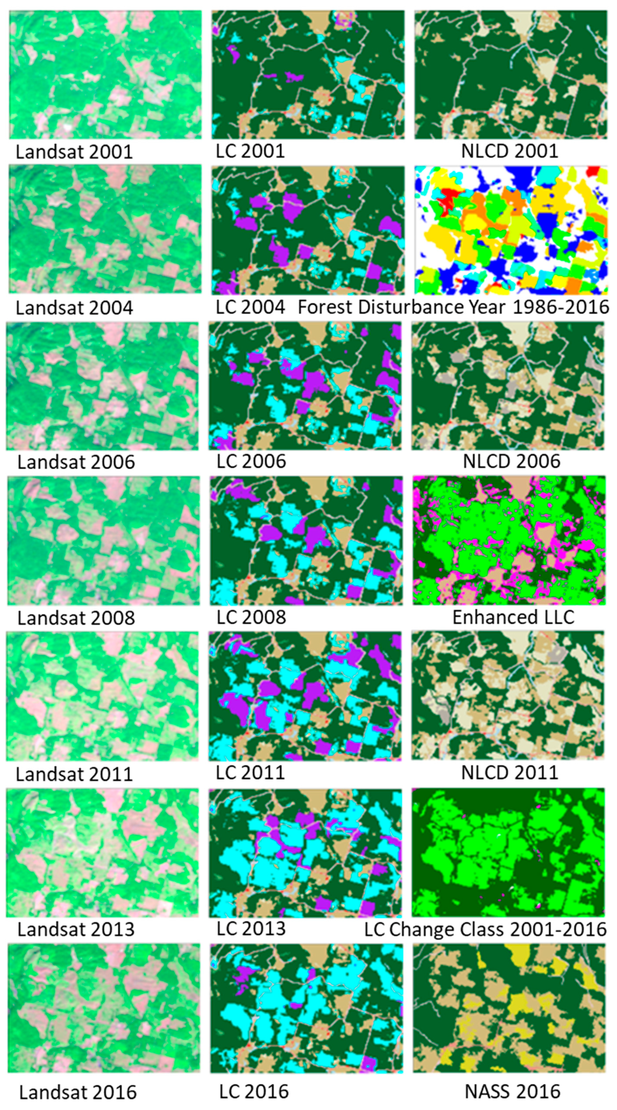
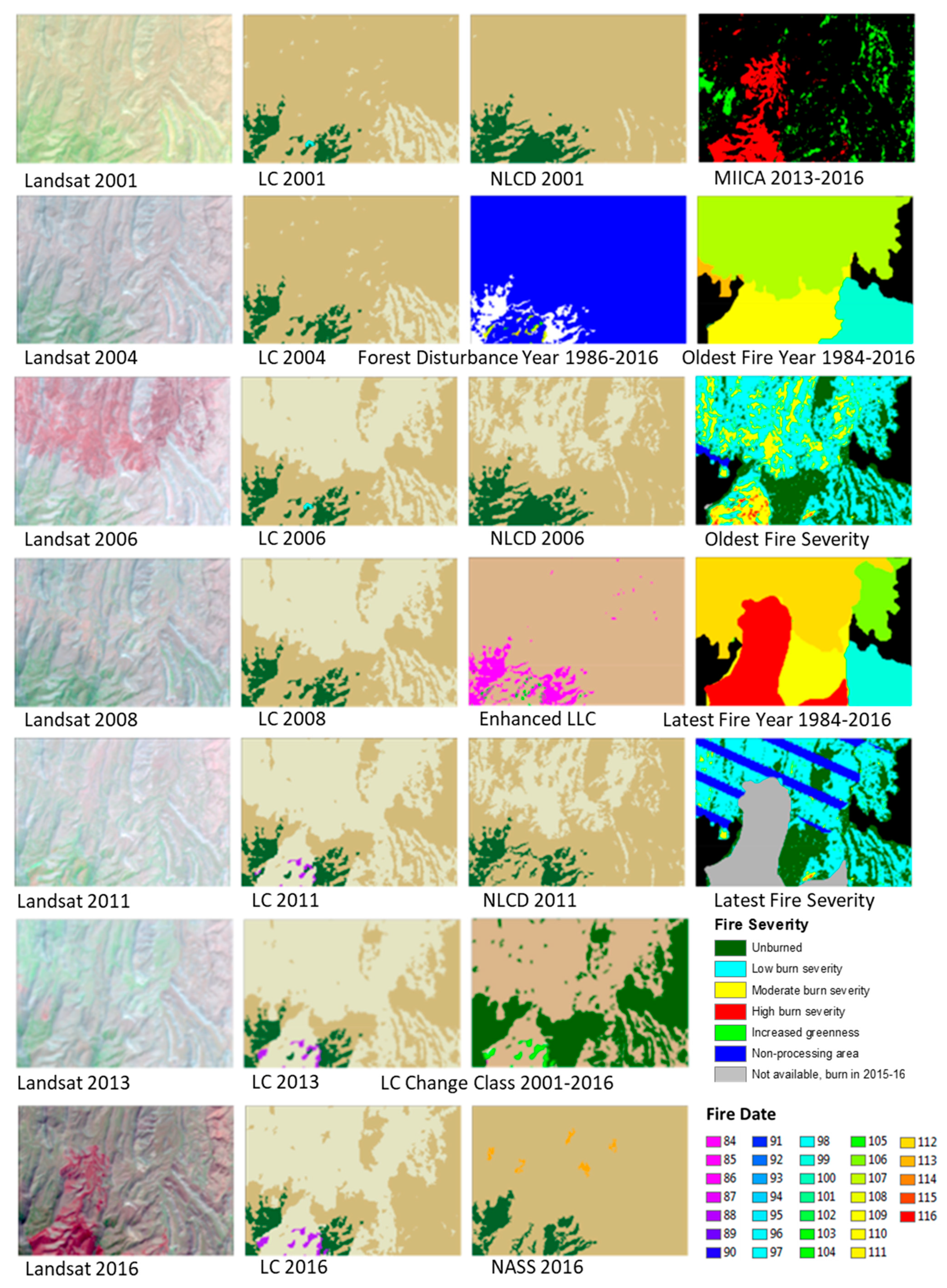
3.1. Results Demonstration

In this section, we present important intermediate and final products from various stages of the process including preprocessing, training data creation, classification, postprocessing, and final integration.
Figure 5 shows an example of Landsat image preprocessing results, with, Figure 5b,d representing the cloud-free results. For each Landsat path/row, eight Landsat images were processed to be completely cloud-free, like the example shown in Figure 5. As a result of Landsat image preprocessing, a total of 3045 Landsat images were processed to be cloud-free for all seven epochs across CONUS. We rely on these Landsat images and ancillary data to produce change detection and land cover mapping products for NLCD.
Figure 6 shows the Landsat images along with some intermediate products used as inputs for training data models. The water product of each Landsat date, generated by our water detection model, matches well to each corresponding Landsat image. In 2001, this area is mainly covered by forests, in 2006, the second Landsat image and water map from the left show a new reservoir, and in 2011, the third Landsat image and water map show the reservoir expansion. This change from forest to water is also evident with the MIICA from 2001–2006 and 2006–2011, which show the new reservoir and its expansion as biomass decrease (BD, in red in Figure 6). The MIICA products show that the forest, urban, and water changes were captured in general with low omission errors, especially for BD change. The fourth row in Figure 6 shows the long-term multi-date change detection results. The forest disturbance year product of 1986–2016 at two- to three-year intervals (the far right panel of the fourth row), which combines VCT ancillary data and the time-series forest disturbance year product from the seven-date Landsat images of 2001–2016, provides information about forest disturbance over a 30-year period and the likely persistent forest area as the class of NoChange (nc, white color in Figure 6). The forest disturbance year product also distinguishes likely non-forest area as the class of disturbed during or before 1986 (blue color in Figure 6) from forest transitional areas, which look similar to each other in Landsat images. The enhanced LLC product (the far right panel of the fifth row) categorizes the area as the primary class of forest-like transitional class (i.e., transiting either from or to forest), then as persistent forest, then some persistent non-forest-like class, and almost no cultivated-crop class. The enhanced LLC product provides the high-level and long-term landscape perspective. Information from each intermediate product provides insights on creating consistent training data for different dates.
For the same example area shown in Figure 6, Figure 7 shows ancillary data inputs for training data models, actual training data, and the initial land cover classifications created for 2001, 2006, 2011, and 2016. Most of those training data are spatially and temporally consistent with each other for the no change area, and the training data for forest-theme classes are dynamically consistent with forest regrowth/succession trajectory. Overall, the initial classification looks reasonable for each individual date.
Figure 8 shows the land cover maps derived from different process stages (i.e., after postprocessing, after final integration, and final released products) for the same area as shown in Figure 6 and Figure 7. Compared to initial land cover classifications, land cover maps after postprocessing are more spatially, temporally, and logically consistent with each other. The land cover maps after final integration, which has integrated spatial-temporal object information, are even more spatially coherent and visually appealing with less salt-and-pepper effects than land cover maps from previous steps. The final integrated land cover maps also adjusted the forest cut areas classified as herbaceous-forest into the managed grassland class (originally NLCD hay/pasture class), which likely will not grow back to forest. The land cover 2001–2016 change classes organized the changes into hierarchical theme-based categories and form an easy-to-view product that summarizes the changes that happened from 2001 to 2016. In this example (Figure 8), the land cover type change map shows that water, forest, and urban are the main disturbance types for this area.

3.2. Examples of Final Land Cover and Land Cover Change Results

Figure 9, Figure 10 and Figure 11 show typical examples of final land cover and change products from the four Landsat path/rows. These examples provide visual examples of how the final seven epoch land cover and land cover change products appear and visual assessments of the quality of new NLCD 2016 products compared to ancillary data.
Figure 9 shows an example of the 7-date final land cover maps and corresponding Landsat images as well as some ancillary data, forest disturbance date of 1986 to 2016, and land cover type change over 15 years for p45r28. In the example area, forest disturbance is dominant, and the forest has been harvested and regenerated by patches over time. Our land cover maps distinguish forest cut areas from persistent shrub areas very well, even though these areas look similar within the same Landsat images. The correct distinctions/classifications relied mainly on the information from forest disturbance year of 1986–2016 and enhanced LLC products.
Figure 10 shows typical fire disturbances on rangeland shrub areas in the western U.S. and demonstrates the use of fire-related ancillary data and expert knowledge on land cover mapping. The impact of fire on Landsat image spectral values can disappear quickly in rangelands in just a few years. However, because fires in these shrubland areas usually reset burned areas to grassland, we employ fire year and fire severity and knowledge of fire succession trajectories in different regions to improve the accuracy of rangeland land cover and land cover change mapping.
Figure 11 shows typical wetland and water change in the Prairie Pothole region and likely Conservation Reserve Program (CRP) lands gradually coming out of conservation easement. Figure 11 also demonstrates the influence of wetland-related ancillary data such as NWI and WPI on wetland and water mapping. The majority of wetland areas were consistently mapped over the years, and mapped water areas match the corresponding Landsat images well. Figure 11 also indicates the impact of agriculture-related ancillary data, such as crosswalked NASS CDL 2016 and Cultivated layer 2009–2015, on agriculture classes mapping. Our cultivated crop areas look more reasonable compared to legacy NLCD and NASS CDL 2016.

3.3. Accuracy Assessment Results

The overall accuracies for the selected four scenes are 82.0% at Level II classification hierarchy (Table 2) and 86.6% at Level I classification hierarchy (Table 3) when results combine either the primary or alternate reference labels. These assessment results are comparable to accuracy results from previous NLCD-generated products (82%, 83%, and 83% at Level II and 88%, 89%, and 89% at Level I for 2011, 2006, and 2001, respectively, in Wickham et al. [53] based on a stratified random sampling assessment). The confusion numbers are the highest between grass (70) and shrub (50) (Table 3). We believe that was caused by several factors, including (1) difficulties in determining the exact type (herbaceous-forest or shrub-forest; rangeland grass or rangeland shrub) during forest and/or rangeland shrub regrowth periods after disturbance, which are natural and continuous processes; (2) lack of high-resolution reference images. If there is a change (e.g., forest cut or fire), the reference label becomes difficult to determine. Either herbaceous-forest (no regeneration after change) or shrub-forest (new regeneration after change) classification may be correct; (3) three out of four path/rows (p18r37, p45r28, and p41r32) we selected having higher disturbance rate between grass (70) and shrub (50) than average and more frequent succession transition; (4) mixed pixels, which represent the boundary of two or several land cover types and abound at the scale of 30-m resolution, resulting in difficulties to identify the dominant land cover. A lot of change patches in our selected path/rows caused more mixed pixels, which makes it more difficult to produce high accuracy maps and to decide on the reference label as well. From Table 4, water (11), high intensity developed (24), evergreen forest (42), shrub/scrub (52), and cropland (82) are produced with higher user’s accuracies (greater than 85%, lower commission error) while water (11), open space developed (21), evergreen forest (42), pasture/hay (81), and cropland (82) are produced with higher producer’s accuracies (greater than 85%, lower omission error).
We also assess the accuracies of binary change/transition and no change/transition classification between each consecutive two epochs (Table 4) at the Level II classification hierarchy. The results show that there is about 3.2% (62/1920) changes across the four scenes for all the change epochs. The producer’s accuracy (66.7%) and user’s accuracy (38.5%) of change classes are relatively lower than the producer’s accuracy and user’s accuracy of the no change classes (both exceed 95%). The producer’s accuracy of change was 44.6%–47.2%, while the user’s accuracy was approximately 82% for all the change periods in 2001–2011 [53]. The difference in accuracies from the two accuracy assessments was probably because of the different distributions of validation samples, the areal extent, the objectives, mapping method, and sampling strategies.
The four Landsat scenes selected for this evaluation are among the most complex places for mapping land cover and land cover change. We chose these four sites in order to rigorously test the NLCD 2016 algorithm. The accuracy evaluation here does not represent the accuracy for the final NLCD land cover products at the national scale. More comprehensive validation will be carried out at the national scale for evaluating the accuracy of the final NLCD 2016 product.

4. Discussion

A spatially detailed and temporally consistent long-term record on land cover status and changes is critical to scientists and stakeholders in assessing natural and human impacts on Earth’s environment, and to carry out climatic, ecological, and natural resource studies and applications at national and global scales. However, at this level of complexity, the high demand for data acquisition and processing, the cost of project execution, and inadequate analytical techniques and methodology often hinder rapid generation of accurate products. This paper reports a new and comprehensive methodology that has been designed and tested to address these issues. Specifically, the developed methods include a streamlined process for assembling and preprocessing Landsat imagery and geospatial ancillary datasets; a multi-source integrated training data preparation and decision tree-based land cover classification process; a temporally, spectrally, and spatially integrated land cover change analysis procedure; and a hierarchical theme-based post-classification and integration protocol for generating land cover and change products.
The below sections highlight salient features of the new NCLD methodology within the context of the large area land cover and change mapping operation.

4.1. Time Series Landsat Image Preprocessing

Unlike any previous NLCD project, NLCD 2016 aims at the development of a long-term, consistent national land cover and land cover change product spanning 15 years. One fundamental requirement for implementing NLCD 2016 is a well-calibrated, spatially and temporally consistent long-term Landsat imagery dataset across the Nation. Although many Landsat image preprocessing methods have been developed, such as image compositing [54] and synthetic image processing [55], few have taken into account both spatial and temporal context simultaneously for image cloud and shadow detection and gap fill. Our research on preprocessing strategies developed improved procedures [39] and resulted in a processing protocol to produce 8-date cloud-free images across the 15-year period for each Landsat path/row for the entire CONUS. Most procedures developed for these steps have been scripted into an automated process to gain operational efficiency.

4.2. Geographic Ancillary Data

Ancillary data are prior knowledge datasets, which are usually derived through collective efforts from an expert team and are likely highly accurate, at least for the focus theme. Geographic ancillary data and local knowledge can be used to improve the accuracy of either classification or the post-classification processes [30,32,56,57,58,59]. For NLCD 2016, we have collected and prepared many ancillary datasets to address different issues related to particular land cover classes. These ancillary data were used not only for developing training data but also for land cover classification and postprocessing. Accuracy assessment results provide compelling evidence that indicates usage of ancillary data has improved overall and class-specific accuracies of the NLCD 2016 prototype product, especially for the wetland class and classes with a land use connotation.

4.3. Training Data for Large Area and Multi-Temporal Land Cover and Change

Many studies demonstrated the importance of high-quality spatially and temporally representative training data for conducting land cover and change classification [32,51,60,61]. The quality of training data is particularly crucial when conducting large-area land cover classification, and insufficient training data are identified as a primary reason for a low accuracy of national or global products when compared to independently collected reference data [62]. For NLCD 2016 research, we have devoted much effort to assemble spectrally, spatially, and temporally consistent training data for each epoch year from 2001 to 2016. Such an approach resulted in a high-quality training dataset that allows spatial and temporal signature extension for mapping land cover and changes at the national scale. Key lessons from our training data creation include: (1) it is feasible to create a large quantity of high-quality training data through modeling and have the training data work well for large-scale classifications; (2), it is essential to target creation of training data for change areas to improve the overall classification accuracy, with trajectory analysis playing an important role in adding training data to change areas; (3), it is important not to remove the training data of edge pixels (i.e., the boundary pixels of landscape patches) because these data are needed to ensure that the land cover label remains stable for those edge pixels over time if no changes occur; and (4) it is also important to create training data according to each land cover theme and to combine those training data in a confidence/priority order.

4.4. Temporal and Spatial Land Cover Characterization and Change Mapping Method

Khatami et al. [57] concluded after their meta-analysis of 266 studies of classification algorithms that inclusion of texture information yielded the greatest improvement in the overall accuracy of land-cover classification with an average increase of 12.1%, and ancillary data was second, yielding an 8.5% increase. For NLCD 2016, we integrated multi-temporal, multi-spectral, and geospatial ancillary data and knowledge to derive seven epoch land cover and change products. We developed targeted strategies and comprehensive models for mapping land cover types and changes beyond the conventional spectral-only change detection and classification.

4.5. Postprocessing

We conducted class-specific postprocessing procedures to improve temporal and spatial accuracy and consistency in class labels over time. Conclusions from previous research call for a post-classification error reduction process [10]. In particular, post-classification error reduction that incorporates knowledge of land cover dynamics and ecological processes is useful when time series land cover maps are generated [63]. In our study, the post-classification process utilized information from spectral and temporal data, spatial context, change trajectory, expert knowledge, and ancillary data to refine the initial land cover and change labels, and corrected errors in each epoch year’s land cover map as well as temporal inconsistency in time series land cover maps. The postprocessing was conducted in a hierarchical order, and different sets of rules and models were developed for each land cover class.
Postprocessing improved the accuracy of the initial land cover label from the seven-date land cover maps and also ensured spatial temporal coherence and consistency on the land cover change products from 2001 to 2016. Temporal information has been demonstrated to be able to add high additional value to change detection and classification [64,65]; however, the spatial domain information of the majority of the time series algorithms is almost entirely ignored [66]. Zhu [66] presents a comprehensive review of change detection algorithms using Landsat time series based on 102 articles published between 2000 and 2016 and points out that a spatial-temporal integrated approach, similar to what we employ here, may be the future direction for change detection.

4.6. Final Integration

A national-scale project such as NLCD 2016 requires careful quality control procedures to ensure high accuracy and consistency of the final products. After postprocessing was completed, the final integration process ensured accurate and coherent spatiotemporal objects across all years from 2001 to 2016. All spatiotemporal objects followed a temporal change (or no change) trajectory in the same way. All pixels within an object belonged to the same land cover class for an epoch year. We integrated pixel-based and object-based land cover maps and achieved a balance between maintaining the coherence of multi-pixel objects for certain land cover types and keeping single-pixel level information for other types. A guideline we followed was to use an object-based approach for mapping change of natural vegetation and agricultural classes to maintain the spatial coherence; to use a pixel-based approach for water, snow/ice and develop classes to retain their spatial details; and to integrate object-based and pixel-based approaches for no change areas [38].

4.7. Constraints and Limitations of NCLD 2016 Methods

Although the methods reported here improved the turnaround time to release seven new epochs of land cover products, some method dependencies and limitations remain. The developed methods rely on relatively perfect imagery to achieve a high accuracy of the final land cover and change products. If the image quality and acquisition time related to vegetation phenology are not optimized, the quality of land cover model output may be compromised. As some model processes rely on ancillary data and/or expert knowledge to determine land cover conditions and changes, uncertainties and errors within these data can negatively affect the spatial, temporal, and thematic accuracies of modeling output. Since so many ancillary data (particularly for CONUS) were used throughout the entire process, it makes the process difficult to be directly applied to other regions where such rich ancillary data are not available. However, the idea of leveraging ancillary data and our descriptions of how ancillary data can be created and used to improve land cover mapping at each processing stage provide helpful insights for other similar projects. The operational unit is still based on one Landsat path/row, which likely impacts the efficiency and may add to the complexity and confusion over the overlap areas of Landsat path/rows. While the entire process, which is composed of over 100 models, is complicated and may be difficult to replicate in other areas, the basic concepts and approach can be applied to other land cover change and mapping cases. Despite these limitations, results from our selected areas confirm the efficacy and robustness of the new method, which has been streamlined and advanced for NLCD 2016 operational national production.

5. Conclusions

This paper reports a new and comprehensive methodology that was designed to create a seven epoch, spatially and temporally consistent, accurate, and up-to-date land cover and change datasets from 2001–2016. The method has been tested and validated using four Landsat path/rows representing a variety of land cover types and land cover changes. The overall accuracies for the four path/rows as a whole are 82.0% at Anderson Level II classification hierarchy and 86.6% at Level I classification hierarchy when matching the map labels with either the primary or alternate reference labels. Using the same protocol for the matching, the overall accuracy of individual scenes varies from 77.9% to 86.8% at Level II.
It is anticipated that NLCD 2016, a nationally consistent time series land cover and change database at 30-m spatial resolution, will revolutionize our understanding of the spatial magnitude and trajectory of land use and land cover change. NLCD 2016 will enable the data producer and user communities to go beyond land cover change detection alone and move toward a more comprehensive scientific understanding of the nation’s land cover dynamics, processes, causes, and consequences in a consistent and credible way [67]. NLCD 2016 will provide insights on a substantial period of past land cover dynamics and provide a foundation for assessing impacts of future changes on the provision and management of land resources and ecosystem service. NLCD 2016 products, which are available for download from www.mrlc.gov, can be used to assess land cover change through time, provide critical input data to a variety of environmental process models, and allow simulation of many natural and anthropogenic processes that are not directly observable.

Author Contributions

Conceptualization, S.J.; methodology, S.J.; validation, C.L. and Z.Z.; formal analysis, S.J.; investigation, S.J.; resources, J.D.; data curation, P.D.; writing—original draft preparation, S.J., L.Y., C.L., Z.Z.; writing—review and editing, C.H., J.D., G.X., D.H.; supervision, S.J. and L.Y.; project administration, J.D.; funding acquisition, C.H.

Funding

This research received no external funding.

Acknowledgments

This work has been performed under the USGS contracts 140G0119C0001 and G15PC00012. The authors wish to thank Lei Ji and Mr. Thomas Adamson for conducting agency internal review. We also would like to thank all the anonymous reviewers for their constructive comments. Any use of trade, product, or firm names is for descriptive purposes only and does not imply endorsement by the U.S. Government.

Conflicts of Interest

The authors declare no conflict of interest.

Appendix A

Table A1. NLCD 2016 Land Cover Class Descriptions for Conterminous United States (CONUS).
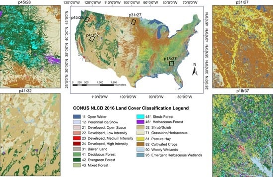
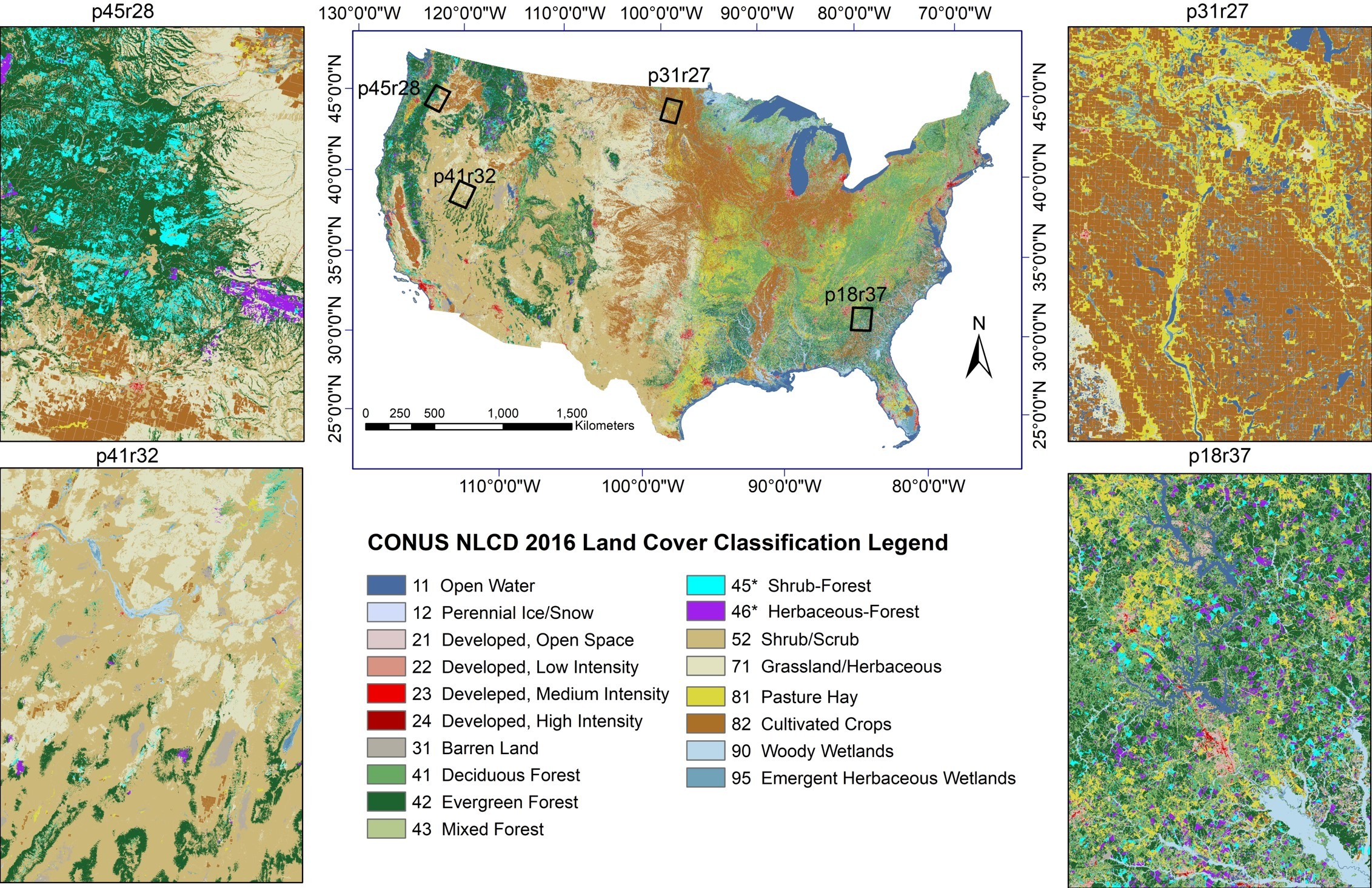
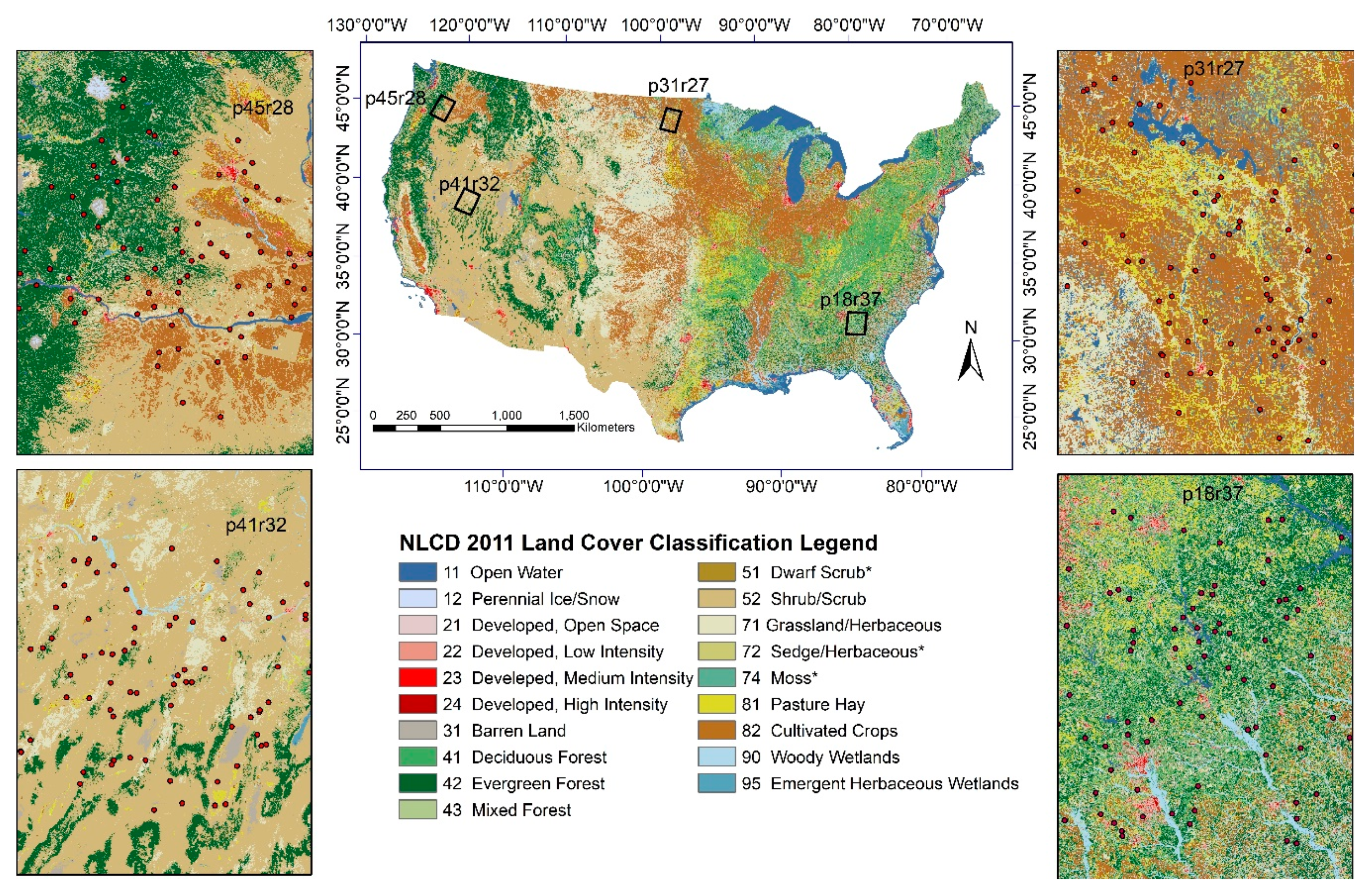
11. Open Water—All areas of open water, generally with less than 25% cover of vegetation or soil.
12. Perennial Ice/Snow—All areas characterized by a perennial cover of ice and/or snow, generally greater than 25% of total cover.
21. Developed, Open Space—Includes areas with a mixture of some constructed materials, but mostly vegetation in the form of lawn grasses. Impervious surfaces account for less than 20 percent of total cover. These areas most commonly include large-lot single family housing units, parks, golf courses, and vegetation planted in developed settings for recreation, erosion control, or aesthetic purposes
22. Developed, Low Intensity—Includes areas with a mixture of constructed materials and vegetation. Impervious surfaces account for 20–49 percent of total cover. These areas most commonly include single-family housing units.
23. Developed, Medium Intensity—Includes areas with a mixture of constructed materials and vegetation. Impervious surfaces account for 50–79 percent of the total cover. These areas most commonly include single-family housing units.
24. Developed, High Intensity—Includes highly developed areas where people reside or work in high numbers. Examples include apartment complexes, row houses, and commercial/industrial. Impervious surfaces account for 80 to100 percent of the total cover.
31. Barren Land (Rock/Sand/Clay)—Barren areas of bedrock, desert pavement, scarps, talus, slides, volcanic material, glacial debris, sand dunes, strip mines, gravel pits, and other accumulations of earthen material. Generally, vegetation accounts for less than 15% of total cover.
41. Deciduous Forest—Areas dominated by trees generally greater than 5 meters tall, and greater than 20% of total vegetation cover. More than 75 percent of the tree species shed foliage simultaneously in response to seasonal change.
42. Evergreen Forest—Areas dominated by trees generally greater than 5 meters tall, and greater than 20% of total vegetation cover. More than 75 percent of the tree species maintain their leaves all year. Canopy is never without green foliage.
43. Mixed Forest—Areas dominated by trees generally greater than 5 meters tall, and greater than 20% of total vegetation cover. Neither deciduous nor evergreen species are greater than 75 percent of total tree cover.
44*. Young-Forest—Areas identified as spectrally having properties of both shrub and forest, likely indicating a transitioning young forest.
45*. Shrub-Forest—Areas identified as current Shrub/Scrub like original Class 52 but showing spectral properties of transitioning to future forest. This class includes trees in a shrub successional stage.
46*. Herbaceous-Forest—Areas identified as current grass like original Class 71 but showing spectral properties of transitioning from being either a past forest or to future shrub-forest. This class includes trees in an early herbaceous successional stage.
52. Shrub/Scrub—Areas dominated by shrubs; less than 5 meters tall with shrub canopy typically greater than 20% of total vegetation. This class includes true shrubs, young trees in an early successional stage or trees stunted from environmental conditions.
71. Grassland/Herbaceous—Areas dominated by grammanoid or herbaceous vegetation, generally greater than 80% of total vegetation. These areas are not subject to intensive management such as tilling but can be utilized for grazing.
82. Cultivated Crops—Areas used for the production of annual crops, such as corn, soybeans, vegetables, tobacco, and cotton, and also perennial woody crops such as orchards and vineyards. Crop vegetation accounts for greater than 20 percent of total vegetation. This class also includes all land being actively tilled.
90. Woody Wetlands—Areas where forest or shrubland vegetation accounts for greater than 20 percent of vegetative cover and the soil or substrate is periodically saturated with or covered with water.
95. Emergent Herbaceous Wetlands—Areas where perennial herbaceous vegetation accounts for greater than 80 percent of vegetative cover and the soil or substrate is periodically saturated with or covered with water.
* New forest transitional classes used in land cover generation. Note these classes are not included in the general land cover release.
Table A2. Descriptions of immediate products used in the training data creation process.
  • Water extent of each year—Water areas detected corresponding to each-epoch Landsat image
  • Snow extent of each year—Snow areas detected corresponding to each-epoch Landsat image
  • Water frequency of 2001–2016—Accumulated water occurrence frequency generated from 7 water extent maps, 2001–2016. This also likely indicates the maximum water extent from 2001 to 2016
  • Snow frequency of 2001–2016—Accumulated snow occurrence frequency generated from7 lsnow extent maps, 2001–2016. This also likely also indicates the maximum snow extent from 2001 to 2016
  • Multi-Index Integrated Change Analysis (MIICA)—A change product derived from two dates of Landsat images with two change classes (biomass increase, biomass decrease), likely indicating areas experiencing high magnitude spectral change between two dates
  • Persistent forest—A product conservatively shows the areas staying as forest without disturbance during 2001 to 2016
  • Normalized Spectral Distance (NSD)—An output identifying the normalized spectral difference of each Landsat pixel to the average spectral values of persistent forest pixels
  • Forest Disturbance year,2001 to 2016—A product created from 7-date multi-temporal change detection, showing the earliest forest disturbance year between 2001 to 2016
  • Forest Disturbance year of 1986 to 2016—A product thatintegrates VCT of 1984–2010 to the Disturbance year of 2001 to 2016 on either areas of no-disturbance or areas disturbed before 2001. This provides information about the forest disturbance date at 2–3 years intervals, as well as likely non-forest and persistent forest areas over the time period 1986–2016.
  • Long-term Land Cover (LLC)—A product derived from the analysis of 7-date NSD temporal pattern, categorizing the landscape from 1986–2016 into four general coarse strata: likely agriculture, likely persistent forest, likely transitional forest, and likely rangeland.
  • Enhanced LLC—A product categorizing the landscape from1986–2016 into five general strata: likely agriculture, likely persistent forest, likely transitional forest, likely rangeland, and uncertain other areas.

References

  1. Foley, J.A.; Defries, R.; Asner, G.P.; Barford, C.; Bonan, G.; Carpenter, S.R.; Chapin, F.S.; Coe, M.T.; Daily, G.C.; Gibbs, H.K.; et al. Global consequences of land use. Science 2005, 309, 570–574. [Google Scholar] [CrossRef] [PubMed] [Green Version]
  2. Houghton, R.A.; House, J.I.; Pongratz, J.; van der Werf, G.R.; DeFries, R.S.; Hansen, M.C.; Le Quere, C.; Ramankutty, N. Carbon emissions from land use and land-cover change. Biogeosciences 2012, 9, 5125–5142. [Google Scholar] [CrossRef] [Green Version]
  3. Running, S.W. Climate change. Ecosystem disturbance, carbon, and climate. Science 2008, 321, 652–653. [Google Scholar] [CrossRef] [PubMed]
  4. Turner, B.L., 2nd; Lambin, E.F.; Reenberg, A. The emergence of land change science for global environmental change and sustainability. Proc. Natl. Acad. Sci. USA 2007, 104, 20666–20671. [Google Scholar] [CrossRef] [Green Version]
  5. Hansen, M.C.; Loveland, T.R. A review of large area monitoring of land cover change using Landsat data. Remote Sens. Environ. 2012, 122, 66–74. [Google Scholar] [CrossRef]
  6. Hansen, M.C.; Potapov, P.V.; Moore, R.; Hancher, M.; Turubanova, S.A.; Tyukavina, A.; Thau, D.; Stehman, S.V.; Goetz, S.J.; Loveland, T.R.; et al. High-resolution global maps of 21st-century forest cover change. Science 2013, 342, 850–853. [Google Scholar] [CrossRef] [Green Version]
  7. Hermosilla, T.; Wulder, M.A.; White, J.C.; Coops, N.C.; Hobart, G.W. Regional detection, characterization, and attribution of annual forest change from 1984 to 2012 using Landsat-derived time-series metrics. Remote Sens. Environ. 2015, 170, 121–132. [Google Scholar] [CrossRef]
  8. Huang, C.Q.; Coward, S.N.; Masek, J.G.; Thomas, N.; Zhu, Z.L.; Vogelmann, J.E. An automated approach for reconstructing recent forest disturbance history using dense Landsat time series stacks. Remote Sens. Environ. 2010, 114, 183–198. [Google Scholar] [CrossRef]
  9. Kennedy, R.E.; Cohen, W.B.; Schroeder, T.A. Trajectory-based change detection for automated characterization of forest disturbance dynamics. Remote Sens. Environ. 2007, 110, 370–386. [Google Scholar] [CrossRef]
  10. Wulder, M.A.; Coops, N.C.; Roy, D.P.; White, J.C.; Hermosilla, T. Land cover 2.0. Int. J. Remote Sens. 2018, 39, 4254–4284. [Google Scholar] [CrossRef] [Green Version]
  11. Witmer, R. Cataract operation and retinal detachment. Mod. Probl. Ophthalmol. 1977, 18, 477–479. [Google Scholar] [CrossRef]
  12. Schroeder, W.; Oliva, P.; Giglio, L.; Quayle, B.; Lorenz, E.; Morelli, F. Active fire detection using Landsat-8/OLI data. Remote Sens. Environ. 2016, 185, 210–220. [Google Scholar] [CrossRef] [Green Version]
  13. Waldner, F.; Canto, G.S.; Defourny, P. Automated annual cropland mapping using knowledge-based temporal features. ISPRS J. Photogramm. Remote Sens. 2015, 110, 1–13. [Google Scholar] [CrossRef]
  14. Yang, L.M.; Xian, G.; Klaver, J.M.; Deal, B. Urban land-cover change detection through sub-pixel imperviousness mapping using remotely sensed data. Photogramm. Eng. Remote Sens. 2003, 69, 1003–1010. [Google Scholar] [CrossRef]
  15. Tulbure, M.G.; Broich, M. Spatiotemporal dynamic of surface water bodies using Landsat time-series data from 1999 to 2011. ISPRS J. Photogramm. Remote Sens. 2013, 79, 44–52. [Google Scholar] [CrossRef]
  16. Vogelmann, J.E.; Howard, S.M.; Yang, L.M.; Larson, C.R.; Wylie, B.K.; Van Driel, N. Completion of the 1990s National Land Cover Data set for the conterminous United States from Landsat Thematic Mapper data and Ancillary data sources. Photogramm. Eng. Remote Sens. 2001, 67, 650. [Google Scholar] [CrossRef]
  17. Fry, J.; Xian, G.S.; Jin, S.; Dewitz, J.; Homer, C.; Yang, L.; Barnes, C.; Herold, N.; Wickham, J. Completion of the 2006 National Land Cover Database for the Conterminous United States. Photogramm. Eng. Remote Sens. 2011, 77, 858–864. [Google Scholar]
  18. Homer, C.; Dewitz, J.; Fry, J.; Coan, M.; Hossain, N.; Larson, C.; Herold, N.; McKerrow, A.; VanDriel, J.N.; Wickham, J. Completion of the 2001 National Land Cover Database for the conterminous United States. Photogramm. Eng. Remote Sens. 2007, 73, 337–341. [Google Scholar]
  19. Homer, C.; Dewitz, J.; Yang, L.M.; Jin, S.; Danielson, P.; Xian, G.; Coulston, J.; Herold, N.; Wickham, J.; Megown, K. Completion of the 2011 National Land Cover Database for the Conterminous United States—Representing a Decade of Land Cover Change Information. Photogramm. Eng. Remote Sens. 2015, 81, 345–354. [Google Scholar] [CrossRef]
  20. Emanuel, R.E. Climate Change in the Lumbee River Watershed and Potential Impacts on the Lumbee Tribe of North Carolina. J. Contemp. Water Res. Educ. 2018, 163, 79–93. [Google Scholar] [CrossRef]
  21. Fertner, C.; Jørgensen, G.; Sick Nielsen, T.A.; Bernhard Nilsson, K.S. Urban sprawl and growth management—Drivers, impacts and responses in selected European and US cities. Future Cities Environ. 2016, 2, 9. [Google Scholar] [CrossRef]
  22. Hu, S.; Niu, Z.; Chen, Y.; Li, L.; Zhang, H. Global wetlands: Potential distribution, wetland loss, and status. Sci. Total Environ. 2017, 586, 319–327. [Google Scholar] [CrossRef] [PubMed]
  23. Kaplan, S.; Peeters, A.; Erell, E. Predicting air temperature simultaneously for multiple locations in an urban environment: A bottom up approach. Appl. Geogr. 2016, 76, 62–74. [Google Scholar] [CrossRef]
  24. Martin, K.L.; Hwang, T.; Vose, J.M.; Coulston, J.W.; Wear, D.N.; Miles, B.; Band, L.E. Watershed impacts of climate and land use changes depend on magnitude and land use context. Ecohydrology 2017, 10. [Google Scholar] [CrossRef]
  25. Smidt, S.J.; Haacker, E.M.K.; Kendall, A.D.; Deines, J.M.; Pei, L.; Cotterman, K.A.; Li, H.; Liu, X.; Basso, B.; Hyndman, D.W. Complex water management in modern agriculture: Trends in the water-energy-food nexus over the High Plains Aquifer. Sci. Total Environ. 2016, 566–567, 988–1001. [Google Scholar] [CrossRef] [Green Version]
  26. Thompson, S.J.; Johnson, D.H.; Niemuth, N.D.; Ribic, C.A. Avoidance of unconventional oil wells and roads exacerbates habitat loss for grassland birds in the North American great plains. Biol. Conserv. 2015, 192, 82–90. [Google Scholar] [CrossRef]
  27. Moigne, J.L.; Grubb, T.G.; Milner, B.C. IMAGESEER: NASA IMAGEs for Science, Education, Experimentation and Research. IEEE Geosci. Remote Sens. Mag. 2013, 1, 44–58. [Google Scholar] [CrossRef]
  28. Dong, J.W.; Kuang, W.H.; Liu, J.Y. Continuous land cover change monitoring in the remote sensing big data era. Sci. China-Earth Sci. 2017, 60, 2223–2224. [Google Scholar] [CrossRef]
  29. Gong, P.; Wang, J.; Yu, L.; Zhao, Y.C.; Zhao, Y.Y.; Liang, L.; Niu, Z.G.; Huang, X.M.; Fu, H.H.; Liu, S.; et al. Finer resolution observation and monitoring of global land cover: First mapping results with Landsat TM and ETM+ data. Int. J. Remote Sens. 2013, 34, 2607–2654. [Google Scholar] [CrossRef] [Green Version]
  30. Chen, J.; Chen, J.; Liao, A.; Cao, X.; Chen, L.; Chen, X.; He, C.; Han, G.; Peng, S.; Lu, M.; et al. Global land cover mapping at 30m resolution: A POK-based operational approach. ISPRS J. Photogramm. Remote Sens. 2015, 103, 7–27. [Google Scholar] [CrossRef] [Green Version]
  31. Zhu, Z.; Woodcock, C.E. Continuous change detection and classification of land cover using all available Landsat data. Remote Sens. Environ. 2014, 144, 152–171. [Google Scholar] [CrossRef] [Green Version]
  32. Zhu, Z.; Gallant, A.L.; Woodcock, C.E.; Pengra, B.; Olofsson, P.; Loveland, T.R.; Jin, S.; Dahal, D.; Yang, L.; Auch, R.F. Optimizing selection of training and auxiliary data for operational land cover classification for the LCMAP initiative. ISPRS J. Photogramm. Remote Sens. 2016, 122, 206–221. [Google Scholar] [CrossRef] [Green Version]
  33. Franklin, S.E.; Ahmed, O.S.; Wulder, M.A.; White, J.C.; Hermosilla, T.; Coops, N.C. Large Area Mapping of Annual Land Cover Dynamics Using Multitemporal Change Detection and Classification of Landsat Time Series Data. Can. J. Remote Sens. 2015, 41, 293–314. [Google Scholar] [CrossRef]
  34. Latifovic, R.; Pouliot, D. Multitemporal land cover mapping for Canada: Methodology and products. Can. J. Remote Sens. 2005, 31, 347–363. [Google Scholar] [CrossRef]
  35. Sexton, J.O.; Noojipady, P.; Anand, A.; Song, X.P.; McMahon, S.; Huang, C.Q.; Feng, M.; Channan, S.; Townshend, J.R. A model for the propagation of uncertainty from continuous estimates of tree cover to categorical forest cover and change. Remote Sens. Environ. 2015, 156, 418–425. [Google Scholar] [CrossRef] [Green Version]
  36. Lambin, E.F.; Geist, H.J.; Lepers, E. Dynamics of land-use and land-cover change in tropical regions. Annu. Rev. Environ. Resour. 2003, 28, 205–241. [Google Scholar] [CrossRef] [Green Version]
  37. Liu, J.Y.; Kuang, W.H.; Zhang, Z.X.; Xu, X.L.; Qin, Y.W.; Ning, J.; Zhou, W.C.; Zhang, S.W.; Li, R.D.; Yan, C.Z.; et al. Spatiotemporal characteristics, patterns, and causes of land-use changes in China since the late 1980s. J. Geogr. Sci. 2014, 24, 195–210. [Google Scholar] [CrossRef]
  38. Rose, Z.B. The enzymology of 2,3-bisphosphoglycerate. Adv. Enzymol. Relat. Areas Mol. Biol. 1980, 51, 211–253. [Google Scholar] [CrossRef]
  39. Jin, S.; Homer, C.; Yang, L.; Xian, G.; Fry, J.; Danielson, P.; Townsend, P.A. Automated cloud and shadow detection and filling using two-date Landsat imagery in the USA. Int. J. Remote Sens. 2012, 34, 1540–1560. [Google Scholar] [CrossRef]
  40. Zhu, Z.; Wang, S.X.; Woodcock, C.E. Improvement and expansion of the Fmask algorithm: Cloud, cloud shadow, and snow detection for Landsats 4-7, 8, and Sentinel 2 images. Remote Sens. Environ. 2015, 159, 269–277. [Google Scholar] [CrossRef]
  41. Zhu, Z.; Woodcock, C.E. Object-based cloud and cloud shadow detection in Landsat imagery. Remote Sens. Environ. 2012, 118, 83–94. [Google Scholar] [CrossRef]
  42. Anderson, J.R.; Hardy, E.E.; Roach, J.T.; Witmer, R.E. A Land Use and Land Cover Classification System for Use with Remote Sensor Data; US Government Printing Office: Washington, DC, USA, 1976; Volume 964.
  43. Homer, C.; Huang, C.Q.; Yang, L.M.; Wylie, B.; Coan, M. Development of a 2001 National Land-Cover Database for the United States. Photogramm. Eng. Remote Sens. 2004, 70, 829–840. [Google Scholar] [CrossRef] [Green Version]
  44. Nussbaum, S.; Menz, G. eCognition Image Analysis Software. In Object-Based Image Analysis and Treaty Verification; Springer: Dordrecht, The Netherlands, 2008; pp. 29–39. [Google Scholar]
  45. Jin, S.M.; Yang, L.M.; Danielson, P.; Homer, C.; Fry, J.; Xian, G. A comprehensive change detection method for updating the National Land Cover Database to circa 2011. Remote Sens. Environ. 2013, 132, 159–175. [Google Scholar] [CrossRef] [Green Version]
  46. Key, C.H.; Benson, N.C. Landscape Assessment: Ground Measure of Severity, the Composite Burn Index; and Remote Sensing of Severity, the Normalized Burn Ratio; RMRS-GTR-164-CD: Ogden, UT, USA, 2006. [Google Scholar]
  47. García, M.J.L.; Caselles, V. Mapping burns and natural reforestation using thematic Mapper data. Geocarto Int. 2008, 6, 31–37. [Google Scholar] [CrossRef]
  48. Rigge, M.B.; Gass, L.; Homer, C.G.; Xian, G.Z. Methods for Converting Continuous Shrubland Ecosystem Component Values to Thematic National Land Cover Database Classes; No 2017-1119; US Geological Survey: Reston, VA, USA, 2017; p. 18. [Google Scholar]
  49. Quinlan, J.R. C4.5: Programs for Machine Learning; Morgan Kaufmann Publishers Inc.: Burlington, MA, USA, 1993; p. 302. [Google Scholar]
  50. Leo Breiman, J.F.; Charles, J.; Stone, R.A. Classification and Regression Trees; Wadsworth International Group: Camden, NJ, USA, 1984; Volume 37, pp. 237–251. [Google Scholar]
  51. Li, C.C.; Wang, J.; Wang, L.; Hu, L.Y.; Gong, P. Comparison of Classification Algorithms and Training Sample Sizes in Urban Land Classification with Landsat Thematic Mapper Imagery. Remote Sens. 2014, 6, 964–983. [Google Scholar] [CrossRef] [Green Version]
  52. Walters, S.P.; Schneider, N.J.; Guthrie, J.D. Geospatial Multi-Agency Coordination (GeoMAC) Wildland Fire Perimeters, 2008; No 612; US Geological Survey: Reston, VA, USA, 2011. [Google Scholar]
  53. Wickham, J.; Stehman, S.V.; Gass, L.; Dewitz, J.A.; Sorenson, D.G.; Granneman, B.J.; Poss, R.V.; Baer, L.A. Thematic accuracy assessment of the 2011 National Land Cover Database (NLCD). Remote Sens. Environ. 2017, 191, 328–341. [Google Scholar] [CrossRef] [Green Version]
  54. Roy, D.P.; Ju, J.C.; Kline, K.; Scaramuzza, P.L.; Kovalskyy, V.; Hansen, M.; Loveland, T.R.; Vermote, E.; Zhang, C.S. Web-enabled Landsat Data (WELD): Landsat ETM plus composited mosaics of the conterminous United States. Remote Sens. Environ. 2010, 114, 35–49. [Google Scholar] [CrossRef]
  55. Zhu, Z.; Woodcock, C.E.; Holden, C.; Yang, Z.Q. Generating synthetic Landsat images based on all available Landsat data: Predicting Landsat surface reflectance at any given time. Remote Sens. Environ. 2015, 162, 67–83. [Google Scholar] [CrossRef]
  56. Brown, J.F.; Loveland, T.R.; Merchant, J.W.; Reed, B.C.; Ohlen, D.O. Using Multisource Data in Global Land-Cover Characterization—Concepts, Requirements, and Methods. Photogramm. Eng. Remote Sens. 1993, 59, 977–987. [Google Scholar]
  57. Khatami, R.; Mountrakis, G.; Stehman, S.V. A meta-analysis of remote sensing research on supervised pixel-based land-cover image classification processes: General guidelines for practitioners and future research. Remote Sens. Environ. 2016, 177, 89–100. [Google Scholar] [CrossRef] [Green Version]
  58. Srinivasan, A.; Richards, J.A. Knowledge-based techniques for multi-source classification. Int. J. Remote Sens. 1990, 11, 505–525. [Google Scholar] [CrossRef]
  59. Vogelmann, J.; Sohl, T.; Howard, S. Regional characterization of land cover using multiple sources of data. Photogramm. Eng. Remote Sens. 1998, 64, 45–57. [Google Scholar]
  60. Mellor, A.; Boukir, S.; Haywood, A.; Jones, S. Exploring issues of training data imbalance and mislabelling on random forest performance for large area land cover classification using the ensemble margin. ISPRS J. Photogramm. Remote Sens. 2015, 105, 155–168. [Google Scholar] [CrossRef]
  61. Millard, K.; Richardson, M. On the Importance of Training Data Sample Selection in Random Forest Image Classification: A Case Study in Peatland Ecosystem Mapping. Remote Sens. 2015, 7, 8489–8515. [Google Scholar] [CrossRef] [Green Version]
  62. Ban, Y.F.; Gong, P.; Gini, C. Global land cover mapping using Earth observation satellite data: Recent progresses and challenges. ISPRS J. Photogramm. Remote Sens. 2015, 103, 1–6. [Google Scholar] [CrossRef] [Green Version]
  63. Gomez, C.; White, J.C.; Wulder, M.A. Optical remotely sensed time series data for land cover classification: A review. ISPRS J. Photogramm. Remote Sens. 2016, 116, 55–72. [Google Scholar] [CrossRef] [Green Version]
  64. Kennedy, R.E.; Andrefouet, S.; Cohen, W.B.; Gomez, C.; Griffiths, P.; Hais, M.; Healey, S.P.; Helmer, E.H.; Hostert, P.; Lyons, M.B.; et al. Bringing an ecological view of change to Landsat-based remote sensing. Front. Ecol. Environ. 2014, 12, 339–346. [Google Scholar] [CrossRef]
  65. Mueller, H.; Rufin, P.; Griffiths, P.; Siqueira, A.J.B.; Hostert, P. Mining dense Landsat time series for separating cropland and pasture in a heterogeneous Brazilian savanna landscape. Remote Sens. Environ. 2015, 156, 490–499. [Google Scholar] [CrossRef] [Green Version]
  66. Zhu, Z. Change detection using landsat time series: A review of frequencies, preprocessing, algorithms, and applications. ISPRS J. Photogramm. Remote Sens. 2017, 130, 370–384. [Google Scholar] [CrossRef]
  67. Sexton, J.O.; Urban, D.L.; Donohue, M.J.; Song, C.H. Long-term land cover dynamics by multi-temporal classification across the Landsat-5 record. Remote Sens. Environ. 2013, 128, 246–258. [Google Scholar] [CrossRef]
Figure 1. Overview of training data creation process for modeling seven dates (2001 to 2016) of land cover.
Remotesensing 11 02971 g001
Figure 2. Overview of major steps to generate initial NLCD land cover mapping products for each target year.
Remotesensing 11 02971 g002
Figure 3. Overview of NLCD 2016 land cover product postprocessing steps. These steps are completed after the initial land cover classification.
Remotesensing 11 02971 g003
Figure 4. Four Landsat path/row and sample areas selected for product accuracy assessment. NLCD 2011 is shown as the background.
Remotesensing 11 02971 g004
Figure 5. A subset example of cloud filled Landsat results. The coordinate of the image center is 83°35′28.643″W 33°25′25.171″N. (a) 2001 Landsat image of p18r37(07/14/2001), (b) the cloud-filled 2001 Landsat image, (c) 2006 Landsat image of p18r37 (07/28/2006), and (d) the cloud-filled 2006 Landsat image.
Remotesensing 11 02971 g005
Figure 6. Landsat images (84°0′11.571″W 33°22′42.752″N is the center coordinate ), ancillary data, and intermediate products developed for training data creation: (1) the first row is preprocessed Landsat images of 2001, 2006, 2011, and 2016 from left to right; (2) the second row is water detection maps corresponding to each Landsat image; (3) the third row is MIICA output of each consecutive image pair, having two values (i.e., biomass increase and biomass decrease); (4) the fourth row is disturbance year (the first panel starting from the left is VCT ancillary data, the second panel is the time-series forest disturbance year product from 7-date Landsat images of 2001–2016, and the third panel is the forest disturbance year product of 1986–2016 at 2- to 3-year intervals by integrating information from first and second files); (5) the fifth row is long-term land cover (the first panel is the combined 2009–2015 Cultivated layer, with dark green representing no cultivated crop across time, the second panel is longer-term land cover (LLC), and the third panel is the enhanced LLC).
Remotesensing 11 02971 g006
Figure 7. The original land cover, training data, and initial classification for the example area: (1) the first row is NLCD 2001, NLCD 2006, NLCD 2011, and NASS CDL 2016 crosswalked; (2) the second row is training data (no training data in the black area) created for 2001, 2006, 2011, and 2016 from left to right; (3) the third row is the initial decision tree classifications for 2001, 2006, 2011 and 2016. There are three new classes (young-forest, shrub-forest, and herbaceous-forest) added to the original NLCD legend.
Remotesensing 11 02971 g007
Figure 8. Land cover at different stages (please refer to Figure 7 for the land cover legend): (1) the first row is land cover of 2001, 2006, 2011, and 2016, each with different land cover theme postprocessing steps; (2) the second row is final integration and some regional adjustment of land cover; (3) the third row is land cover, which is the final released product where the young-forest class was crosswalked into other classes; and (4) the fourth row is the land cover change classes summarized over 2001–2016 associated with the 7-date land covers.
Remotesensing 11 02971 g008
Figure 9. An example from p45r28 (image center coordinate is 121°22′38.784″W 45°49′49.162″N) with Landsat image, ancillary data, and new land cover and change products (please find legends in the previous figures): (1) the first column is the Landsat image of 2001, 2004, 2006, 2008, 2011, 2013, and 2016 from top to bottom; (2) the second column is the new final land cover of 2001, 2004, 2006, 2008, 2011, 2013, and 2016 from top to bottom; (3) the third column is NLCD 2001, forest disturbance year of 1986 to 2016, NLCD 2006, enhanced LLC, NLCD 2011, land cover 2001–2016 change class, and crosswalked NASS CDL 2016.
Remotesensing 11 02971 g009
Figure 10. An example from p41r32 (center coordinate is 117°32′59.213″W 39°49′56.074″N) with Landsat image, ancillary data, and new land cover and change products: (1) the first column is the Landsat image of 2001, 2004, 2006, 2008, 2011, 2013, and 2016 from top to bottom; (2) the second column is the new final land cover of 2001, 2004, 2006, 2008, 2011, 2013, and 2016 from top to bottom; (3) the third column is NLCD 2001, forest disturbance year of 1986 to 2016, NLCD 2006, enhanced LLC, NLCD 2011, land cover 2001–2016 change class, and crosswalked NASS CDL 2016; (4) the fourth column is MIICA 2013–2016, oldest fire year from 1984 to 2016, severity of the oldest fire, latest fire year from 1984 to 2016, and severity of the latest fire.
Remotesensing 11 02971 g010
Figure 11. An example from p31r27 (center coordinate is 98°44′51.827″W 47°36′55.192″N) with Landsat image, ancillary data, and new land cover and change products: (1) the first column is the Landsat image of 2001, 2004, 2006, 2008, 2011, 2013, and 2016 from top to bottom; (2) the second column is the new final land cover of 2001, 2004, 2006, 2008, 2011, 2013, and 2016 from top to bottom, (3) the third column is NLCD 2001, forest disturbance year of 1986 to 2016, NLCD 2006, enhanced LLC, NLCD 2011, land cover 2001–2016 change class, and crosswalked NASS CDL 2016; (4) the fourth column is crosswalked NWI, Cultivated layer 2009–2015, and WPI.
Remotesensing 11 02971 g011
Table 1. Ancillary data prepared and used for National Land Cover Database (NLCD) 2016 land cover and land cover change production.
Prepared Ancillary DataData SourcePreparation
NLCD legacy data: NLCD 2001, 2006, 2011https://www.mrlc.gov/updated road network data incorporated into NLCD
National Agricultural Statistics Service (NASS) Cropland Data Layer (CDL) 2016https://www.nass.usda.gov/Crosswalked into NLCD classes
NASS Cultivated layer 2009–2015https://www.nass.usda.gov/Combined 2009–2013, 2011–2015 NASS Cultivated layer to extend the time period
National Wetland Inventory (NWI) https://www.fws.gov/Crosswalked NWI into NLCD classes
Hydric Soil https://www.nrcs.usda.gov/Mosaicked tiles into a national map
Wetland Potential Index (WPI)Created in house (USGS NLCD)
The index has already been adopted for LCMAP (Zhu et al., 2016)
A 7-ranking class of wetland potential created by using the convergence of evidence from NWI, Hydric Soil, and NLCD 2011.
Vegetation Change Tracker (VCT) from 1984 to 2010https://www.landfire.gov/Mosaicked tiles into a national map and converted it into a disturbance-year map at 2–3-year intervals.
Existing Vegetation Type (EVT) 2001https://www.landfire.gov/Crosswalked into Anderson level I and climax-class like classes
Shrub crosswalkCreated in house (by USGS NLCD Shrub project)
https://www.mrlc.gov/
Developed models to crosswalk percentage shrub, herbaceous, barren, and other components from Shrub project products into NLCD classes (shrub, herbaceous, barren)
Fire from 1984 to 2016
(1) Fire_year_oldest
(2) Fire_year_latest
(3) Fire_intensity_oldest
(4) Fire_intensity_latest
(5) Fire_frequency
https://www.mtbs.gov/
https://www.geomac.gov/
Developed models to integrate each-year fire from 1984 to 2014 from MTBS, and 2014–2016 fire from GeoMAC to produce five ancillary data related with fire year and severity
Fire_recovery_zoneCreated in house (by USGS NLCD Shrub project)Created a CONUS map with four fire zones with different vegetation recovery rates according to precipitation, ecoregion, and DEM
Fire_recovery_forest_zoneCreated in house (USGS NLCD)Created a map for the western U.S. with ten zones with different recovery rates for forest after fire according to assessment and opinions from experts
Digital Elevation Model (DEM) and derivatives (aspect, cti, slope)https://nationalmap.gov/Removed some artifacts from DEM and calculated derivatives from smoothed DEM
Wetland_boundariesCreated in house (USGS NLCD)Created a CONUS map with 6 wetland zones which characterize different kind of wetland change dynamics according to expert knowledge
Shrub_boundaryCreated in house (USGS NLCD)Created a CONUS map with two zones which roughly separate CONUS into west shrub and east forest regions according to expert knowledge
Sage_dominated_regionCreated in house (by USGS NLCD Shrub project)Created a map that indicates the area where sage shrub likely dominates according to expert knowledge
Percent Imperviousness maps of 2001, 2006, 2011, and 2016https://www.mrlc.gov/Created by independent NLCD urban mapping efforts to provide developed classes and changes over time
Table 2. Accuracy assessment for all NLCD target years across the four path/row scenes at Level II classification hierarchy. In this confusion matrix and following accuracy tables, Prod and User are producer’s and user’s accuracies, respectively, when the primary reference labels match with all map results during 2001–2016. Aprod and Auser are the producer’s and user’s accuracies, respectively, with agreement defined as a match between the map and either the primary or alternate reference labels. The diagonal numbers were highlighted and shaded gray to show the times of points that were correctly classified (i.e., match with the primary reference labels) over seven epochs.
Reference
1121222324414243527181829095TotalUser (%)Auser (%)
Map116100000007000077581.3100.0
210567007000707008466.775.0
22021070000000000280.050.0
230000700000000070.00.0
24000070000000007100.0100.0
41000003212257000007642.161.8
4200000132315393000038184.889.2
43000001412210000004744.774.5
5207000441343041000052681.790.1
7100000560141119400027543.359.3
81000001500044138190722361.976.2
8228000000741035602140887.395.1
907000002039002174942.957.1
9520000000077107215438.961.1
Total72927714783966463423415939228632240
Prod (%)84.760.90.00.050.041.081.632.867.850.986.890.875.033.3 70.8
Aprod (%)89.388.766.70.050.070.187.454.777.667.195.593.780.078.6 82.0
Table 3. Accuracy assessment for all NLCD target years across the four path/row scenes at Level I classification hierarchy. Refer to Table 2 for table descriptions.
Reference
10204050708090TotalUser (%)Auser (%)
Map10610070077581.3100.0
2001057077012683.388.9
40004554630050490.393.9
500748430410052681.790.1
7000111411194027543.359.3
8028157485232863182.991.0
90902316175610354.466.0
Total72120538634234551912240
Prod (%)84.787.584.667.850.994.961.5 78.1
Aprod (%)89.399.191.077.667.197.088.3 86.6
Table 4. Confusion matrix for NLCD change detection between each consecutive two epochs (2001–2004, 2004–2006, 2006–2008, 2008–2011, 2011–2013, 2013–2016). Refer to Table 2 for table descriptions.
Reference
No Change/TransitionChange/TransitionTotalUser (%)Auser (%)
MapNo change/transition180240184297.899.2
Change/transition56227828.238.5
Total1858621920
Prod (%)97.035.5 95.0
Aprod (%)97.466.7 96.7

