Geo-Object-Based Land Cover Map Update for High-Spatial-Resolution Remote Sensing Images via Change Detection and Label Transfer

Abstract

Land cover (LC) information plays an important role in different geoscience applications such as land resources and ecological environment monitoring. Enhancing the automation degree of LC classification and updating at a fine scale by remote sensing has become a key problem, as the capability of remote sensing data acquisition is constantly being improved in terms of spatial and temporal resolution. However, the present methods of generating LC information are relatively inefficient, in terms of manually selecting training samples among multitemporal observations, which is becoming the bottleneck of application-oriented LC mapping. Thus, the objectives of this study are to speed up the efficiency of LC information acquisition and update. This study proposes a rapid LC map updating approach at a geo-object scale for high-spatial-resolution (HSR) remote sensing. The challenge is to develop methodologies for quickly sampling. Hence, the core step of our proposed methodology is an automatic method of collecting samples from historical LC maps through combining change detection and label transfer. A data set with Chinese Gaofen-2 (GF-2) HSR satellite images is utilized to evaluate the effectiveness of our method for multitemporal updating of LC maps. Prior labels in a historical LC map are certified to be effective in a LC updating task, which contributes to improve the effectiveness of the LC map update by automatically generating a number of training samples for supervised classification. The experimental outcomes demonstrate that the proposed method enhances the automation degree of LC map updating and allows for geo-object-based up-to-date LC mapping with high accuracy. The results indicate that the proposed method boosts the ability of automatic update of LC map, and greatly reduces the complexity of visual sample acquisition. Furthermore, the accuracy of LC type and the fineness of polygon boundaries in the updated LC maps effectively reflect the characteristics of geo-object changes on the ground surface, which makes the proposed method suitable for many applications requiring refined LC maps.

1. Introduction

Land use and land cover change (LUCC) has always been the main tool to investigate and update the Earth surface resources and environment, and it is also the basis of geographical research and applications in remote sensing [1]. Land use (LU) refers to the use, protection, and transformation of land under the guidance of certain purpose and the production modes, in terms of the natural and social attributes of the surface and the laws of resources and the environment. LU emphasizes the role of artificial utilization. Land cover (LC) refers to the cover and time sequence changes formed by the comprehensive influence of nature and man on the surface land, which embodies the complex of natural formation and human intervention. Therefore, the classification systems of LU and LC are relevant but different. This paper pays more attention to the land information of LC whose change has been a hot topic in land resources research. This has important impacts on other environmental issues such as biodiversity, water, carbon, and nutrient cycling, energy balance, and increased greenhouse gas emissions in terrestrial ecosystems. Thus, accurate LC products are important and basic for climate change, the hydrological cycle, and biodiversity conservation simulations [2,3,4]. The emergence of remote sensing technology provides a vital role for the timely and accurate acquisition of LC information [5]. Especially with the opening of the Google Earth Engine (GEE) platform in recent years, geospatial data, including a variety of remote sensing data, strongly support the monitoring and mapping of LC change [6,7].

In the past thirty years, artificial visual interpretation methods based on remote sensing images have become the main way to obtain these products. However, this method cannot meet the current requirements of timeliness, which is mainly manifested in the following: (1) the automatic degree of interpretation of remote sensing images is low, and there is a lack of comprehensive and unified visual interpretation standards; (2) there is a phenomenon of misclassification and omission, which is limited by the professional background and level of operators. In the past ten years, with the technological development of artificial intelligence (AI), machine learning (ML) algorithms in LC classification have improved the automation of classification. These methods, such as neural network (NN), support vector machine (SVM), and decision tree (DT), have been widely employed in LC remote sensing classification by synthetically utilizing the essential features of remote sensing images, such as spectrum, shape, geometric structure, and texture, as well as the relationship between classification units [8]. The development of these classification methods has greatly satisfied the increasing amount and speed of LC information extraction.

However, in the process of ML-based classification, the efficiency and accuracy of remote sensing image interpretation are highly dependent on the LC training samples. The obtainment of training samples is still based on artificial field visits or visual interpretation of remote sensing images. For example, 379 sample areas in global soil data products CD-ROM contents (IGBP-DIS) were interpreted by 39 remote sensing experts in two weeks [9]. Most of the recent works have been performed in analogous ways. For instance, Szantoi et al. used a Global Positioning System (GPS) equipment to conduct a field investigation of Everglades National Park in Florida, USA [10]. A total of 66,430 pixels were obtained as training samples in their model. It can be seen that manual sample collection is laborious and time consuming, and cannot meet the automation requirements of rapid applications. Furthermore, the ability of remote sensing data acquisition is increasing, resulting in a large amount of observation data [8]. Thus, for large-scale classification mapping tasks, it will take vast time and manpower to label the samples, which restricts the interpretation speed of large-scale remote sensing areas. This also reduces the timeliness of remote sensing technology in emergency monitoring [11,12]. Moreover, it is difficult to quickly collect sufficient and accurate samples in a manual way, which will affect rapid LC mapping and change detection with multitemporal remote sensing images [13]. Therefore, the question of how to quickly produce high-quality samples has become an urgent problem for large-scale remote sensing LC classification [14,15].

In addition, it should be noted that previously collected samples contain important prior knowledge for a new task with a target image. However, these historical archived samples cannot be directly reused for current target images. The main reason for this is that the spectral features of the prior samples generally do not follow the statistical probability distribution of the data in the target image (i.e., the spectral-drift phenomenon). That is, due to the influence of atmospheric scattering and absorption, phenology, and other factors, the spectrum of similar objects in different remote sensing images (i.e., different domains) cannot obey an identical statistical probability distribution [16]. However, traditional ML classification algorithms are based on the assumption that data samples are independent and identically distributed (i.i.d.), which cannot be directly applied in domains with different statistical probability distributions. The domain adaptability of existing algorithms is poor, and there is a lack of an effective strategy to reuse historical samples [17]. Thus, if we do not re-label new training samples to meet the training requirement of the current target image classification task, then we will not be able to deploy the traditional classification algorithms. Meanwhile, as pointed out above, the labeling of new samples will consume a lot of manpower and time. Consequently, the acquisition of training samples has become an important factor restricting the development of remote sensing image automatic interpretation. The efficient acquisition of training samples suitable for target images is the prerequisite to promote the accuracy and efficiency of large-scale high-spatial-resolution (HSR) remote image classification.

Although historical samples cannot be directly used to establish the model of the current target image classification task for the above reasons, the prior information and knowledge contained therein are still helpful to the classification of the current target image.

Transfer learning is a ML method that has been put forward in recent years to solve these domain adaptation problems via reusing existing information and knowledge [18,19,20,21]. This theory provides a novel way to solve the problem of sample selection in remote sensing classification via relaxing two hypotheses in traditional ML: (1) training samples and testing samples satisfy the condition of i.i.d.; (2) sufficient training samples should be utilized to learn a robust model. This model is based on the given data sets and learning tasks in the source domain, and mining its knowledge to help complete or perfect the learning tasks in the target domain. Recently, some scholars have carried out research in this field for the target recognition of remote sensing images, LC classification, and other fields through the reuse of samples [16,22,23,24,25,26,27,28,29,30,31]. For example, Bruzzone and Marconcini proposed an LC map updating strategy based on a domain-adaptive SVM [16]. Liu et al. presented a classification method based on case-based reasoning and TrAdaboost for the spatiotemporal information reuse of remote sensing images [29].

Admittedly, these methods have achieved fairly good experimental results in local areas. However, most of the current methods in these studies are designed by directly introducing a transfer learning algorithm from the ML domain, and the geoscience characteristics are considered to be fewer. Such characteristics mainly focus on directly reusing the historical sample resources by modifying the probability distribution of sample features to adapt to the domain of the target images, without considering the invalid samples incorrectly introduced by historical samples. In fact, for a fixed area, historical LC maps have been published for many time periods [11,32]. However, the rich geoscience knowledge in these historical maps has not been fully exploited and applied for LC classification of later phases [4,17,33]. The lack of schemes to reuse previous LC maps results in a waste of historical resources in existing algorithms. Therefore, the question of how to transfer the prior knowledge in previous LC maps to the target models and thereby assist in the classification of current target images is a new entry point to improve the efficiency and accuracy of classification with remote sensing images.

Mining invariant objects from existing LC maps and guiding the automatic extraction of samples are of great significance to improve the automation and accuracy of LC classification [25]. This can be considered as the problem of how to carry out automatic and rapid LC map updating in the same area with the support of historical LC maps. In 2010, MRLC, a multiresolution land characterization agency in the United States, used the old and new phases of medium-resolution remote sensing images to detect the changing areas, and used the automatic sample selection method to realize the automatic classification of the new phase of images. This efficiently completed the updating of the national surface coverage database (NLCD) and the thematic data of impervious surface [11]. The global high-resolution remote sensing mapping carried out in China also draws on the above research ideas [12]. Through these works, we can see that the transfer of prior knowledge from previous maps to the target model is feasible in this LC map update framework. However, most of these studies commonly employed pixel-based processing in their transfer learning-based LC research with medium-resolution remote sensing data, such as Landsat satellite data. In order to avoid the salt-pepper noise of pixel-level methods, it is necessary to update LC information based on geo-object units for HSR images. Therefore, aiming to resolve the problem whereby pixel samples are susceptible to noise, we propose an efficient LC map update approach at a geo-object scale for HSR remote sensing. An automatic method of collecting training samples from historical LC maps through combining change detection and label transfer is designed in this paper, as we aware that change detection can quickly inherit invariant ground objects’ LC class information. A data set with Chinese Gaofen-2 (GF-2) HSR satellite data is constructed to evaluate the performance of our method. The experiment results with these data show that the algorithm can automatically obtain reliable geo-object-level samples for classification in target images. The method demonstrates effectiveness for automatic LC map updating. The specific objectives of this study were to: (1) use historical data to update LC information quickly via designing the ideas and requirements of automatic sample collection; (2) apply HSR remote sensing images based on the basic scale of geo-objects; (3) discuss the potential impacts of several details in our proposed method.

2. Materials and Methods

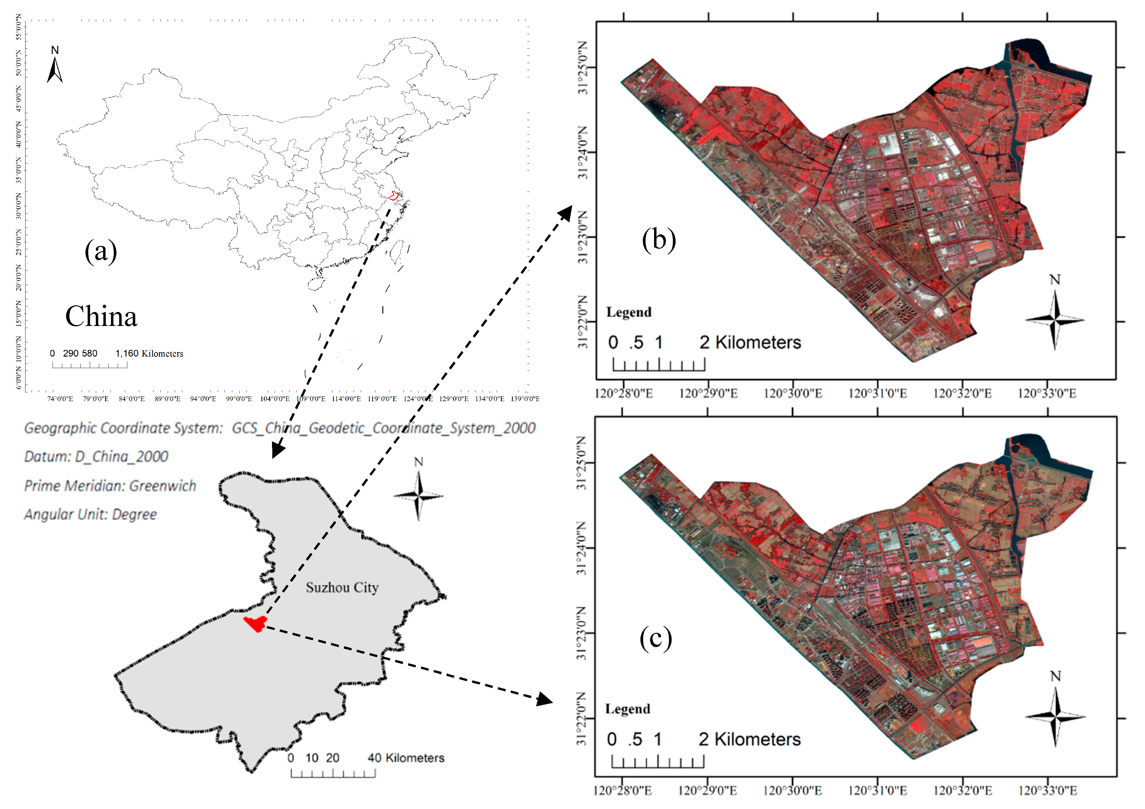
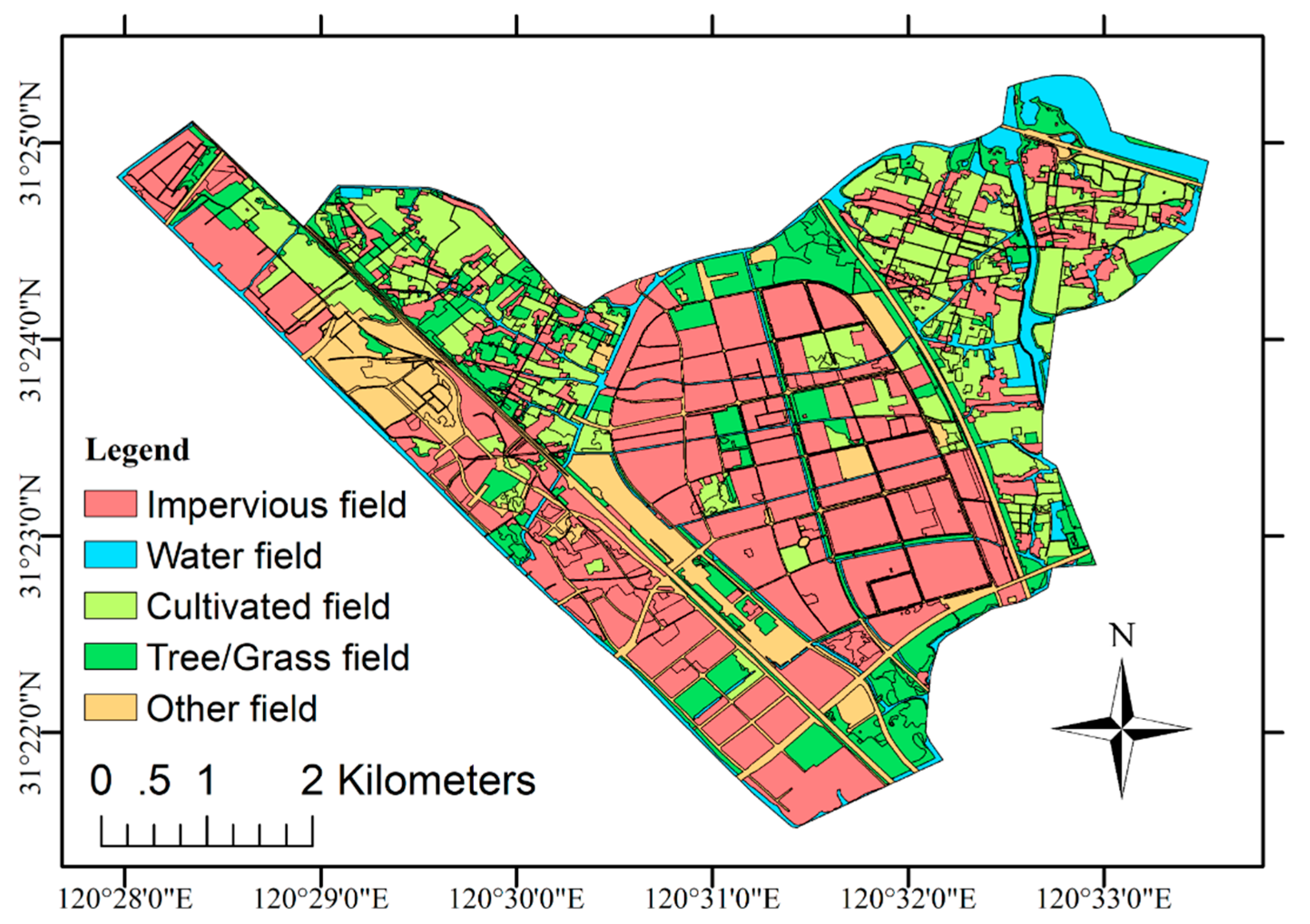
2.1. Data Set

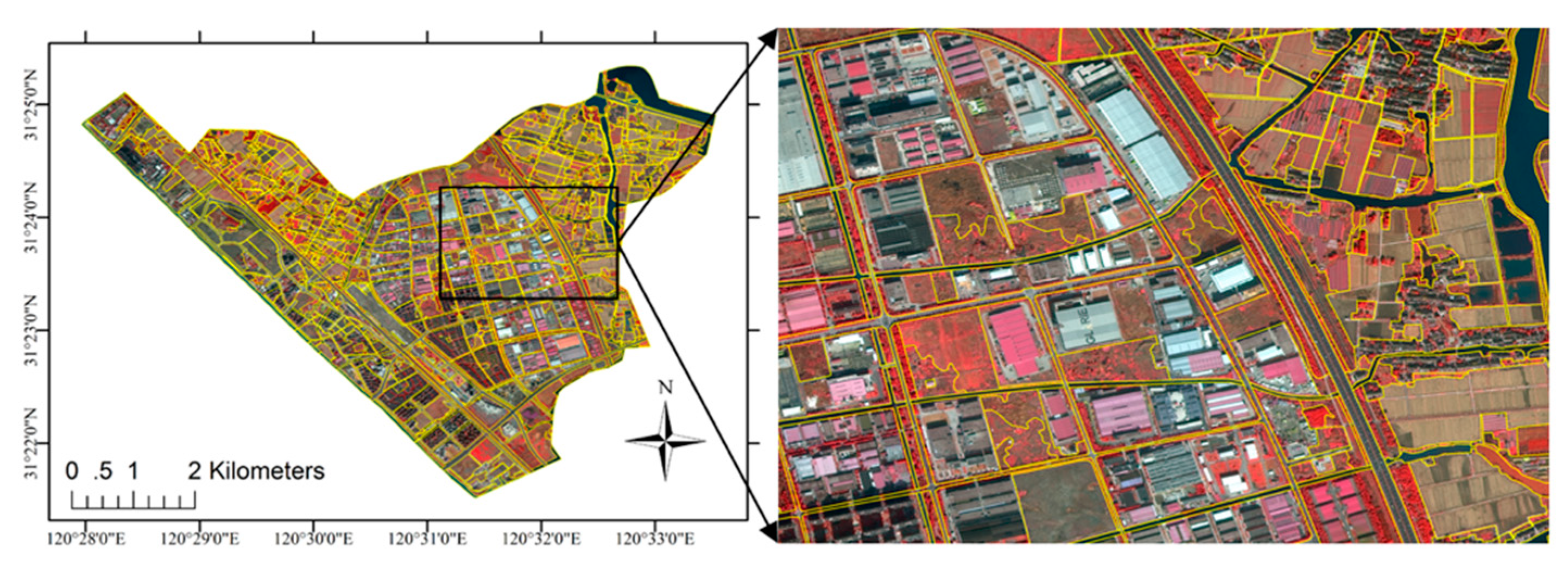
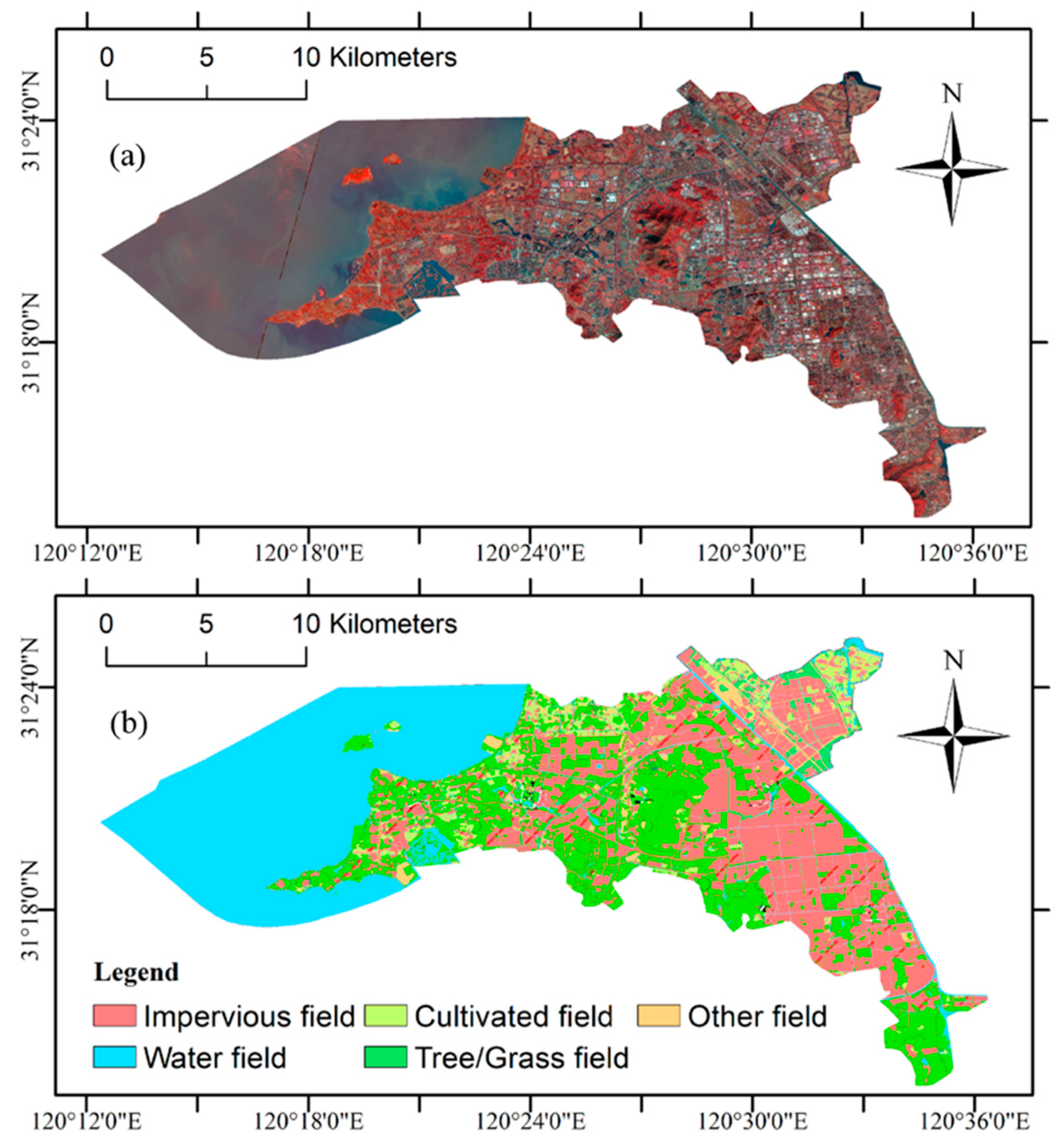
2.1.1. Remote Sensing Images

Two GF-2 remote sensing images are selected for this experiment. GF-2 is an optical satellite with two cameras, a 1-m resolution panchromatic camera and a 4-m resolution multispectral camera (see

Table 1. Sensors’ technical specifications of the GF-2 satellite.

Band No.		Spectral Range (μm)	Spatial Resolution (m)	Swath Width (km)	Repetition Cycle (days)
Panchromatic band	0	0.45–0.90	1	45 (two cameras combined)	5
Multispectral bands	1	0.45–0.52	4
	2	0.52–0.59
	3	0.63–0.69
	4	0.77–0.89

). Thus, its fusion data from panchromatic and multispectral bands have high spatial resolution, with 0.8 m at sub-satellite points. Figure 1 shows the 4-3-2 band composition in the fusion data (0.8-m spatial resolution and 12,906 × 8860 pixels). The images were acquired in the subarea of Gaoxin District, Suzhou City, Jiangsu Province, China, on 23 July 2016 and 15 October 2018, respectively. The image in the year 2016 (i.e., Figure 1b) is referred to as the reference image of the first phase (T₁), while the image in the year 2018 (i.e., Figure 1c) is referred to as the target image of the second phase (T₂). Then, image registration and relative radiation normalization procedures were performed on these fusion data.

2.1.2. Ancillary Data

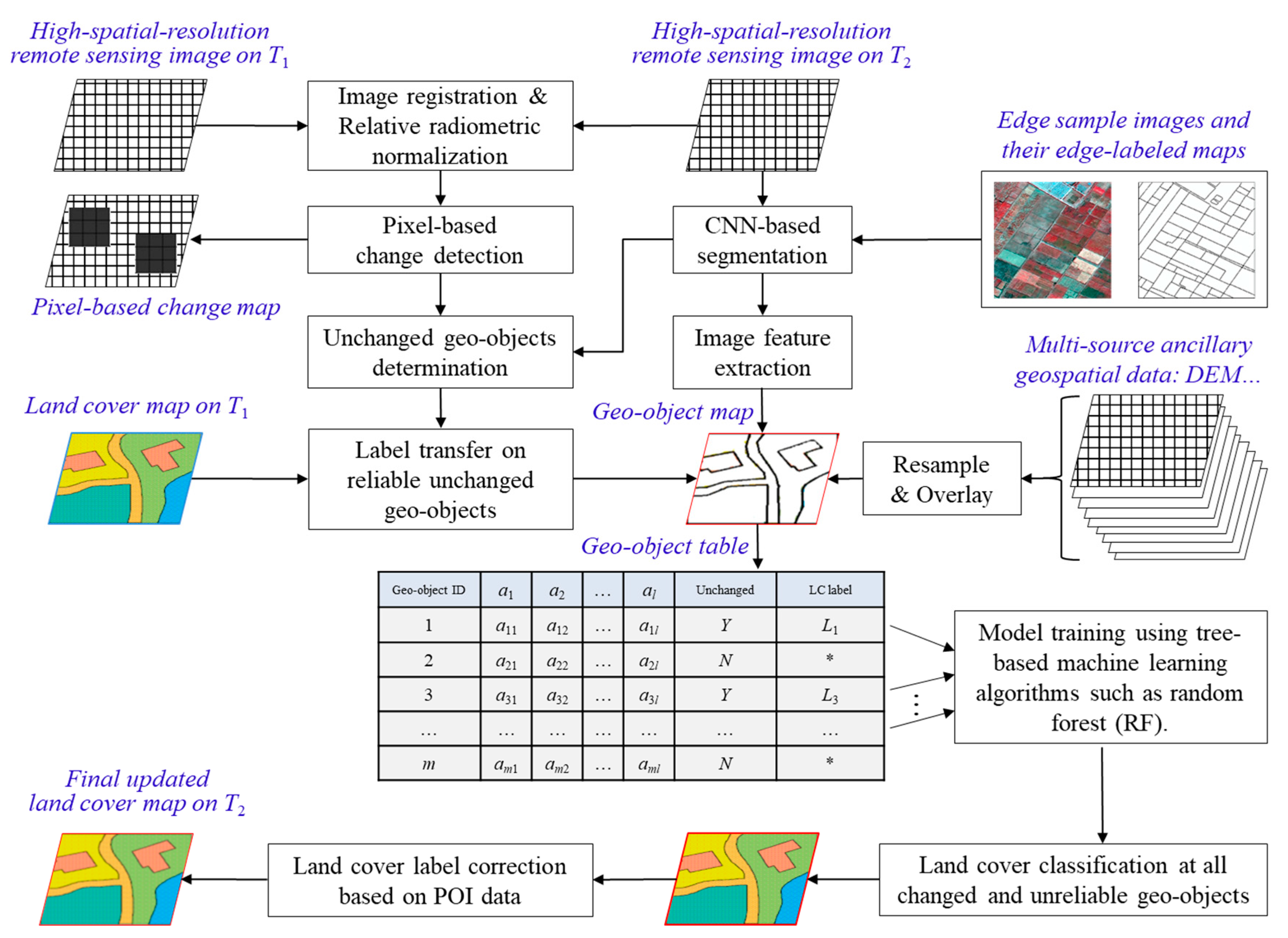
For the ancillary data in our approach, a historical (previous first phase, i.e., 2016) LC map (see Figure 2), in accordance with Figure 1b, is first chosen to be updated. Cultivated field, tree/grass field, impervious field, and water field are the main LC types in this area. In addition, the second version of 30-m Advanced Spaceborne Thermal Emission and Reflection Radiometer Global Digital Elevation Model (ASTER GDEM V2) data is utilized for the orthorectification of GF-2 data and derived terrain features for the follow-up supervised learning. Furthermore, points of interest (POI) data is also collected for post-processing in our procedure.

2.2. Methodology

In this paper, we propose a geo-object-based LC map update method, which focuses on an automatic scheme of object-level training sample collection using previous LC maps. This is called the geo-object-based automatic land cover update (Auto-LCU) method and includes the following procedures as shown in Figure 3.

First, we apply registration and relative radiometric normalization to two-temporal (T₁ and T₂) remote sensing images (called the reference/old image I₁ and the target/new image I₂) of the same area. This is essential for accurate change detection. In our process, geometric registration is guaranteed by the data provider (i.e., product-ready), while a simple panoramic linear regression method is conduct for relative radiation normalization. That is, the image I₁ is linearly normalized according to the reference image I₂ via the band correction one by one. Then, a pixel-based change map is generated via unsupervised change detection between these two images. Then, we aim to solve the problems based on geo-objects, which are referred as basic units for updating LC maps. Therefore, image segmentation using a convolutional neural network (CNN) method is carried out for extracting geo-objects in the target image I₂. The reason why we choose the image I₂ to produce the segmentation image-objects is that our task is to obtain a new LC map of T₂ with the help of the LC data in the former time. The generated polygons from the image I₂ are referred as minimum mapping units for display. Therefore, this is a processing task oriented by LC update, rather than a direct LC change detection task. Image features of extracted geo-objects can then be calculated for the follow-up training.

Second, unchanged geo-objects are further determined using rules designed in Section 2.2.3. The class labels in the LC map of T₁ (i.e., the historical LC map) can then be transferred to all unchanged geo-objects. Among these, some reliable geo-object samples for LC classification of the target image I₂ are automatically selected with the assistance of the first-phase LC map. Then, a structured geo-object table is formatted by integrating the pre-extracted image features and multisource ancillary geospatial data into each geo-object. This results in a standardized data set for ML. Thus, after training on samples using ML algorithms, the relationships between the geo-objects’ conditional features and LC class labels are established. An LC map can be updated for all changed and unreliable geo-objects by utilizing the relationships from the supervised classification algorithm.

Finally, based on the results of the second step, we correct some LC labels using the information of POI data, which are centrally distributed in the construction/building areas. The updated LC map of T₂ is then finally produced. Next, we introduce several key steps in detail.

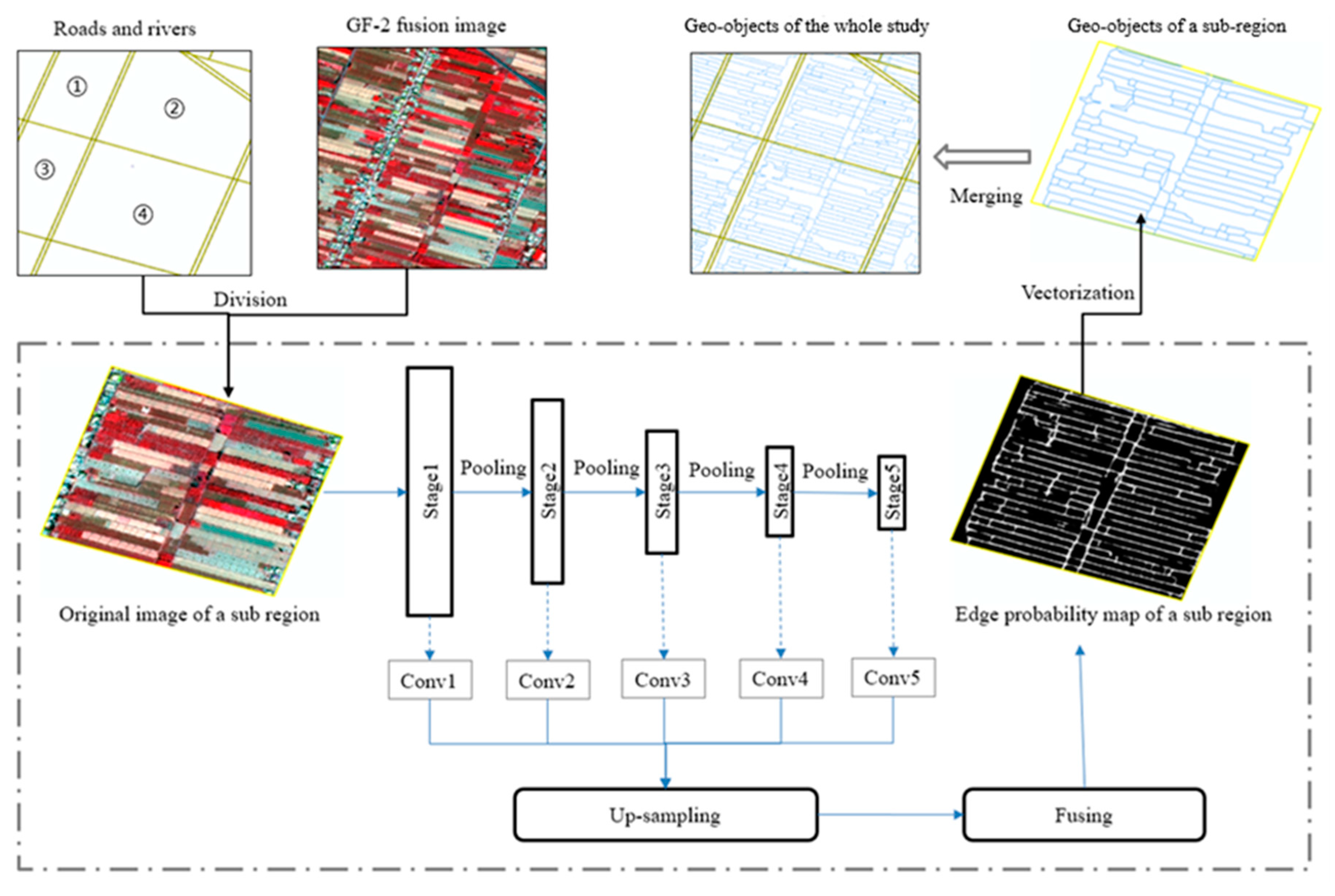
2.2.1. Geo-Object Extraction

In our framework, we use the geo-objects as the smallest spatial unit for mapping, whose vector polygons can be extracted from HSR remote sensing images using segmentation methods. These internally homogeneous geographic objects are employed as the basic update units in this study. Conventionally, multi-scale segmentation is used to generate homogeneous image objects and extract the corresponding polygon vectors [34,35]. Recently, supervised segmentation methods using CNN have been proven feasible for extracting the edge information of objects via self-learning features from images [36]. Hence, in [37], we proposed a CNN-based method for extracting geo-objects from GF-2 fusion images, which is designed as follows (see Figure 4). First, the polygons of roads and rivers in a historical LC map are used to zone the target HSR image into several sub-regions for subsequent processing. That is, the following edge extraction of these sub-region images from division can be conducted in a parallelization mode. Second, we extract an edge probability map for each sub-region using a modified VGG16 network [38]. In this network, five stages of convolution layers are up-sampled and fused by an improved fusion loss layer based on the reference [37,39]. Third, we employ a vectorization on the edge probability map. The boundary of each geo-object’s polygon is then extracted from the sub-region images. All sub-region results are combined to structure a whole geo-object map.

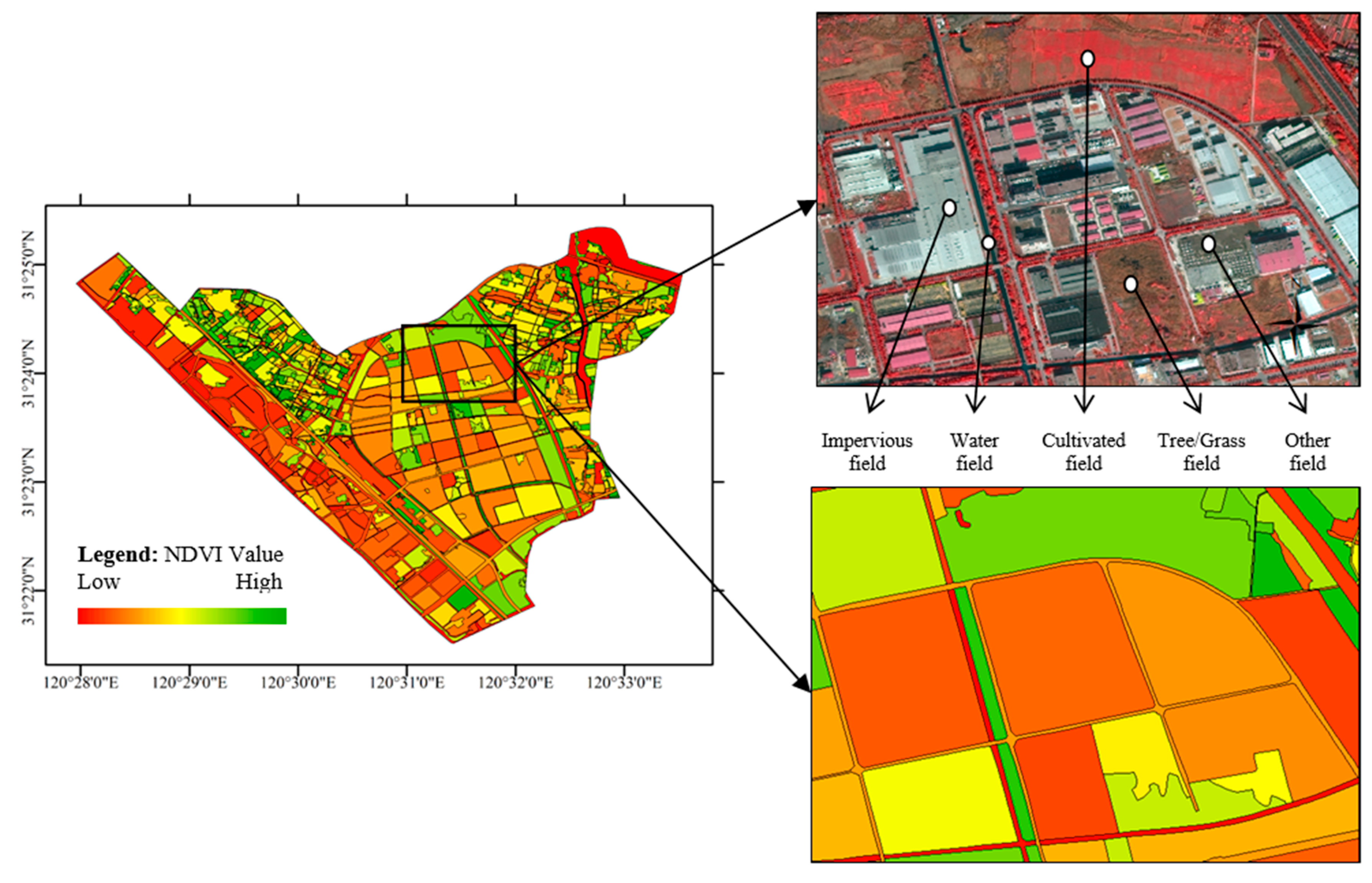
2.2.2. Feature Extraction

After the shape extraction of the geo-object, features extraction is further carried out on each geo-object. In our method, each geo-object corresponds to a data record, and the features designed here are extracted from the relevant data for classification. Here, we focus on the image features of spectrum, shape and texture. First, the mean, standard deviation, brightness and maximum differences of spectral signals, normalized difference vegetation index (NDVI), and normalized difference water index (NDWI) are employed as spectrum features in our extraction. These indexes are calculated from the high-spatial-resolution image bands (one value per pixel), and the mean values on the corresponding pixels covered by each geo-object are employed as features of the geo-object. Second, the main direction, length–width ratio, pixel shape index (PSI) [40], and shape index [41] are calculated as shape features of geo-objects. Third, the texture-derived built-up presence index (PanTex) [42,43] and measures of the gray-level co-occurrence matrices (GLGM) [44] are extracted as the texture features of geo-objects. In addition, terrain features, including mean topographic elevation, slope and aspect, are calculated from digital elevation model (DEM) data. Similarly, these features extracted from DEM-based raster data are one value per pixel. The average values of the pixels covered by each geo-object are taken as its features. In

Table 2. List of geo-object features used in ML.

Spectrum Features	Shape Features	Texture Features	Topographic Features
Mean of spectrum signals in band 1	Length–width ratio	Homogeneity	Elevation
Mean of spectrum signals in band 2	Length of geometry	Contrast	Slope
Mean of spectrum signals in band 3	Width of geometry	Dissimilarity	Aspect
Mean of spectrum signals in band 4	Compactness	Second moment
Standard deviation of spectrum signals in band 1	Main direction of geometry	Entropy
Standard deviation of spectrum signals in band 2	Number of points	Correlation
Standard deviation of spectrum signals in band 3	Length of border
Standard deviation of spectrum signals in band 4	Shape index
Brightness of spectrum signals	Number of corner points
Maximum differences of spectrum signals
Normalized difference vegetation index (NDVI)
Normalized difference water index (NDWI)

, we list the four classes of extracted features, which will be input into ML algorithms. Figure 5 presents a graph showing instances of the NDVI feature for the selected LC types with the units of geo-objects. Other multisource ancillary geospatial data can be further overlaid onto the geo-objects, and more features can be generated reflecting the Earth surface’s LC characteristics and change.

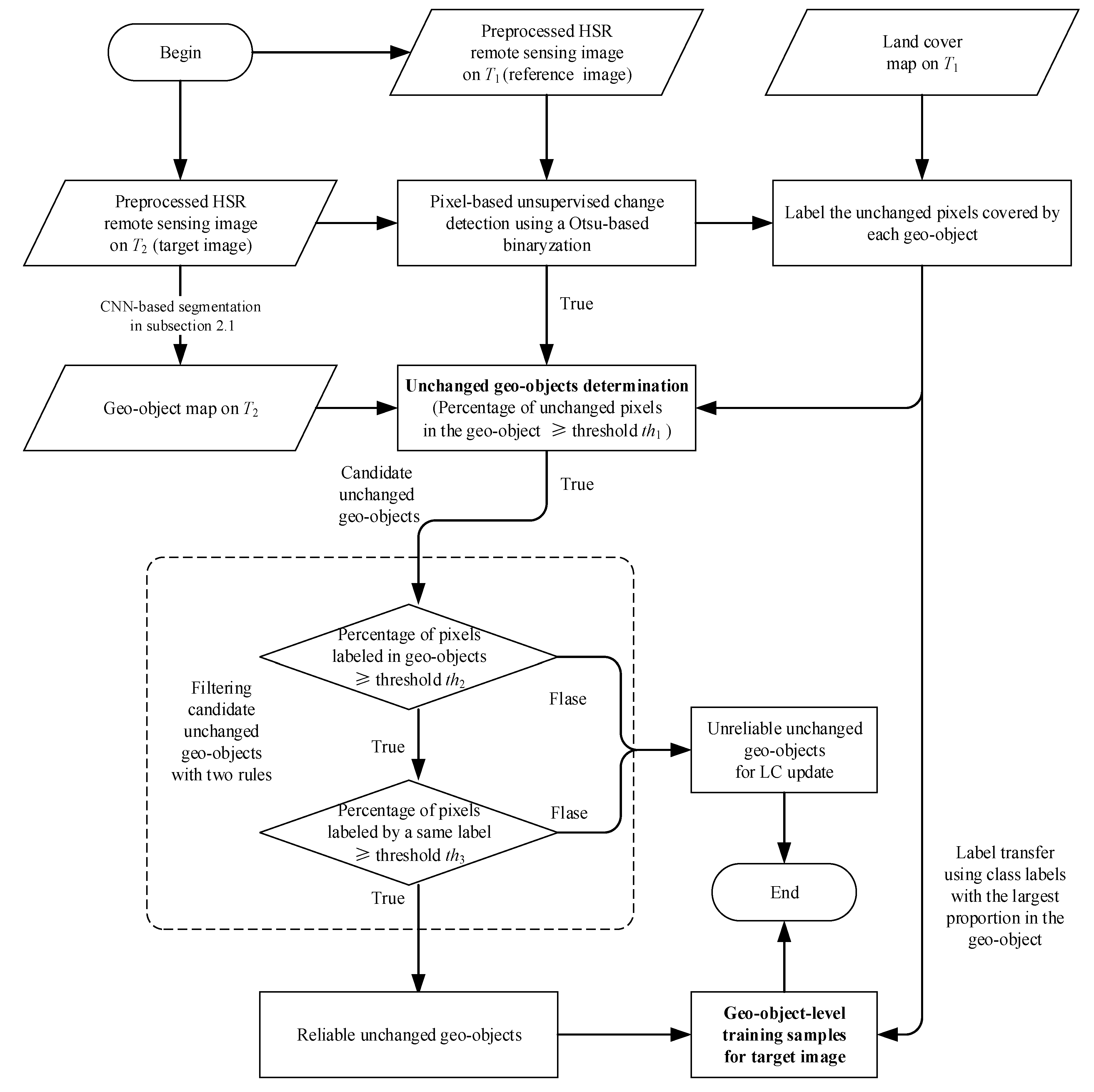
2.2.3. Automatic Scheme of Sample Collection using Change Detection and Label Transfer

Training samples are the source of knowledge to distinguish LC classes in supervised learning. Hence, here, an automatic collection scheme of geo-object-level samples is designed on the target images based on a historical LC map. The basic foundation is that the LC classes of an area do not change much in a short period. That is, most of the LC classes of geo-objects are unchanged in neighboring years. If we can collect a foregone LC map (it may be out of date and needs to be updated), the positions, spatial distribution, and LC labels of the unchanged geo-objects in this map are reliable prior knowledge for the follow-up update. Under this assumption, we design the sample collection scheme using change detection and label transfer, which takes previously interpreted LC maps as a reference. The locations, distribution, and LC labels of unchanged geo-objects are utilized in sample labeling on target images.

The scheme is implemented according to Figure 6. First, pixel-based unsupervised change detection is conducted on images I₁ and I₂. In our experiments, the intensity of change is measured by change vector analysis (CVA), and the binarization is realized using an Otsu’s thresholding method [45,46,47]. We mark the locations of unchanged pixels on the image I₂, and unchanged geo-objects are determined by judging whether the percentage of unchanged pixels in the geo-object is greater than a given threshold th₁. These unchanged geo-objects, through checking the proportion of unchanged pixels in their coverage areas, are referred as candidate objects for training samples. Second, prior labels from the LC map of T₁ are totally linked to the unchanged pixels of the image I₂. Third, three rules with thresholds th₂ and th₃ for filtering unchanged geo-objects are employed to select more reliable geo-objects. That is, the percentage of pixels labeled in each geo-object and the percentage of pixels labeled by the same label are required to be simultaneously higher than the given thresholds th₂ and th₃. Geo-objects that do not satisfy these thresholding rules will be filtered out and cannot be selected as training samples. Under these constraints, the pixels’ LC class labels with the highest proportion in the reliable unchanged geo-objects are transferred as their labels. These threshold setting will be discussed in Section 3.2.1. Finally, geo-object-level training samples with prior labels are rapidly collected in a large-scale area for the LC classification of the target image. Thus, we obtain a structured geo-object-based table with several labeled training samples. The unlabeled geo-objects in this table will be updated via classification.

2.2.4. Geo-Object-Based Supervised Classification

To accurately update the changed LC information, we further conduct a geo-object-level supervised learning by using the collected training samples with their 30-dimensional feature vectors (see Table 2). Here, a tree-based random forests (RF) algorithm is employed for training in our framework due to its robustness in generating prediction functions via high-dimension learning. Detailed descriptions of this algorithm can be found in the literature [48]. After the training step, supervised geo-object-oriented LC classification is conducted to predict LC labels for all unlabeled geo-objects (i.e., unsampled geo-objects, including changed and unreliable unchanged geo-objects). The number of class-labels generated in our method is five general LC types in Figure 2 (i.e., impervious field, water field, cultivated field, tree/grass field, and other field). The LC labels of geo-objects will be totally obtained, and an updated LC map of T₂ can be produced with final label correction using POI data in the study area. POI mainly refers to some geographic entities closely related to people’s life, such as schools, banks, supermarkets, etc. Such POIs describe the spatial and attribute information of these geographic entities, such as the name, address, coordinates, and classes of the entities. Hence, POIs can greatly enhance the ability to describe the location of entities and reflect urban activities. In this step, we contrast the POI classes on the spatial location of the geo-objects with the LC types we identify. If there is not a match, we correct our classification labels according to the information of POI classes. This is effective because most POI data are located in building areas and can indicate the impervious surface of LC information.

3. Results Analysis and Discussions

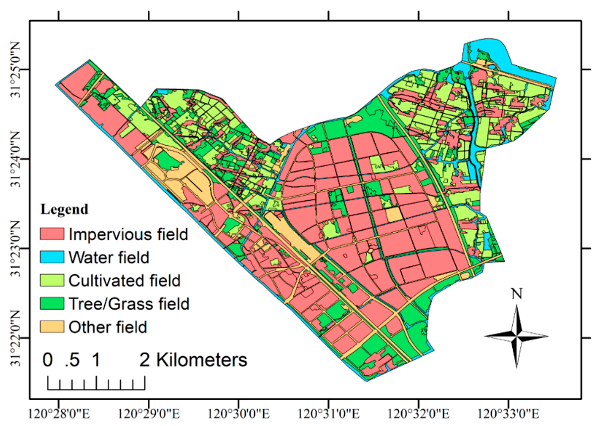
3.1. Experimental Results

In this paper, the target image (i.e., Figure 1c) is input to segment polygons of geo-objects using the method in Figure 4. Figure 7 shows the GF-2 image and simple instances of geo-objects (i.e., the yellow polygons). As shown in Figure 7, the GF-2 fusion data with 0.8-m spatial resolution can accurately depict the surface information in detail, and the 1338 polygons of geo-objects are performed along the edges of land parcels. These are referred to as the smallest units for the subsequent LC map update.

The change detection technology is then conducted by comparing Figure 1b,c. Based on the auxiliary data of Figure 2, geo-object samples are rapidly collected according to Figure 6. In our experiments, all the three proportion thresholds in Figure 6 are set as the same value th = 0.85 for the convenience of computation, i.e., th₁ = th₂ = th₃ = 0.85. That is, the rules are described in the following aspects: (1) the percentage of unchanged pixels in the geo-objects is higher than 85%; (2) the percentage of labeled pixels in the geo-objects is higher than 85%; and (3) the proportion of labeled pixels with the same labels is higher than 85%. The distributions of the selected training geo-object samples for the target image are shown in Figure 8 from the reliable unchanged geo-objects. Then, the unlabeled geo-objects in Figure 8 can be further classified according to the training of these collected samples, and an updated LC map can finally be obtained via post-correction of POI data (see Figure 9). The results in Figure 9 obviously display that the LC labels of some changed geo-objects are intuitively updated.

In order to quantitatively evaluate the accuracy of the updated results, we collected some verification points via a field survey in November 2018. Five thousand verification points (1000 points/class × 5 classes) were randomly picked out in this area. All the points in their geo-objects were located, and the LC classes of these points (i.e., ground truth) were labeled via visual interpretation. In order to improve the objectivity, the labelling was repeatedly sampled three times by different interpreter. Then, we compared the label accuracy using a confusion matrix (

Table 3. Confusion matrix of the LC update using the proposed geo-object-based Auto-LCU method.

LC Class	Number of Artificially Interpreted Points					Producer Accuracy (%)
	Impervious Field	Water Field	Cultivated Field	Tree/Grass Field	Other Field
Impervious field	956	2	3	34	5	95.6
Water field	0	987	1	12	0	98.7
Cultivated field	4	1	894	40	61	89.4
Tree/Grass field	6	3	21	950	20	95.0
Other field	0	1	1	33	965	96.5
User accuracy (%)	99.0	99.3	97.2	88.9	91.8	—
Overall measures	Overall accuracy (OA) (%): 95.22			Kappa coefficient (KC): 0.9324

) and a statistical table (

Table 4. Statistical table of itemized accuracy of each LC class for the proposed geo-object-based Auto-LCU method.

LC Class	Number of Artificially Interpreted Points	Number of Correctly Classified Points	Accuracy (%)	Main Misclassification
Impervious field	1000	956	95.6	Tree/Grass field
Water field	1000	987	98.7	Tree/Grass field
Cultivated field	1000	894	89.4	Tree/Grass field + Other field
Tree/Grass field	1000	950	95.0	Cultivated field + Other field
Other field	1000	965	96.5	Tree/Grass field
Total	5000	4761	95.22	—

). The results show that the majority of LC classes can be accurately updated. Although the accuracy of cultivated field is not high (89.4%), the accuracy of water field is relatively high (98.7%). The accuracies of impervious field, tree/grass field, and other field are also all higher than 95% (95.6%, 95.0%, and 96.50%, respectively). The kappa coefficient (KC) and overall accuracy (OA) are 0.9324 and 95.22%, respectively, which illustrates that the proposed method can automatically update LC information with a reliable performance. Therefore, it is a feasible procedure for updating LC maps in an automatic manner.

3.2. Discussions

The quantity and quality of training samples in supervised LC classification have an important influence on classification accuracy. The conventional visual method via man–machine interaction is high-cost, time-consuming and thus cannot be adapted to meet the needs of the current time efficiency. In order to solve the problem of lack of automation in the process of LC update, this paper proposes an automatic collection method of classification samples based on historical LC data. On this basis, we construct an automatic architecture for LC update. The experimental results in the previous section show that it makes full use of the characteristics of high confidence of classification accuracy in the spatially consistent area of historical LC data, and reduces the impact of invalid samples on classification accuracy through some criterion about spatial heterogeneity in Figure 3. On this set of methods, we will make further discussion on the following issues.

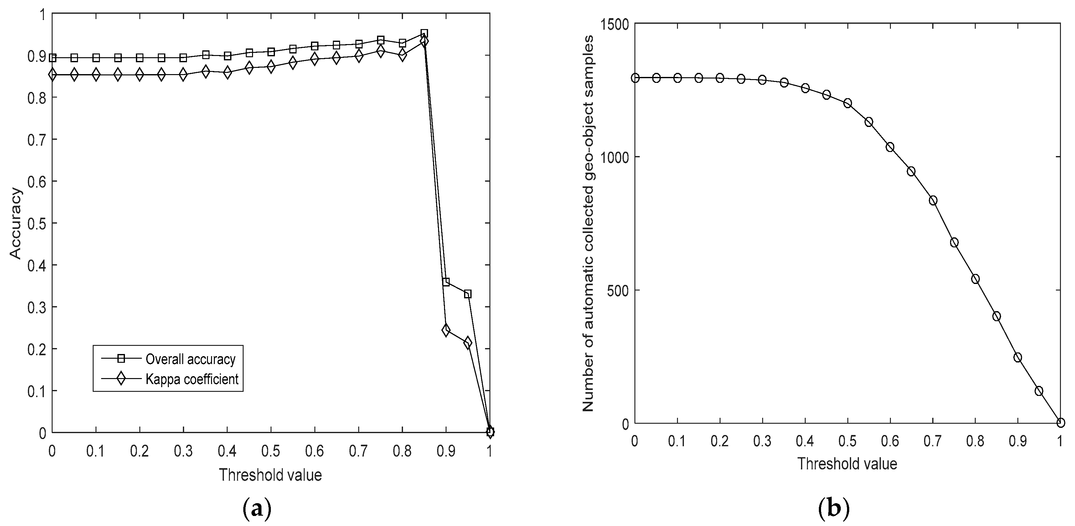
3.2.1. Impact of the Threshold Setup

The thresholds in Figure 6 are critical parameters in the proposed geo-object-based Auto-LCU algorithm. The issue of how to set the parameters so that the algorithm has a better ability to express the characteristics of the LC map update is a focus of the proposed procedure. In the experiments, the three proportion thresholds are set as the same value th for the convenience of computation, i.e., th₁ = th₂ = th₃ = th. Then, the influence of the threshold th on the reported results is further discussed via analyzing the effect on the update accuracy with the change of its threshold value. We also choose the presented data set as the experimental data for this study and set the threshold value in the range from 0.0 to 1.0. As presented in Figure 10a, the accuracies of the updated results under these setups are assessed using OA and KC. Figure 10b shows the change in geo-object sample size via automatic collection with different threshold values.

Figure 10a suggests that the update accuracy increases with the increase in threshold value when it is less than 0.85 and decreases when the threshold value is greater than 0.85. This process is divided into the following stages. First, when the threshold is too small, the rules of sample collection in Figure 6 are weak. This makes the number of automatically selected samples large (see Figure 10b), and the classification accuracy is relatively low as some impure samples are mixed in with the training set. Then, with the increase in threshold value, the rules of sample collection in Figure 6 are gradually strengthened, and the number of automatically selected samples decreases (see Figure 10b). This means that the purity of selected samples is gradually improved, and the classification accuracy also increases. When the threshold value reaches 0.85, the classification accuracy reaches the optimal value. At this point, the sample size is 401, OA is 95.22%, and KC is 0.9324. However, when the threshold value continues to increase, the classification accuracy drops sharply. There are two reasons for this phenomenon. On the one hand, when the threshold value is greater than 0.85, the rules of sample collection in Figure 6 are too strict and thus the selected samples are very few (e.g., the sample size is 247 for th = 0.9, 122 for th = 0.95, and 2 for th = 1.0, see Figure 10b). A small sample size will seriously affect the robustness of the classification. On the other hand, there is a large label-imbalance in the sample set when the threshold value is greater than 0.85. It may even occur that almost no samples of a certain class are selected (e.g., when th = 1.0, only two samples are collected), which leads to a sharp decline in Kappa coefficients in the final classification results. In particular, there is a sharp decrease in Figure 10a when threshold value changes from 0.85 to 1.0. The main reason for this phenomenon is that, after the threshold value is greater than 0.85, there is an increasing imbalance in the automatically collected samples. In our experiment, the sample numbers of other field, water field, and impervious field are far less than those of cultivated field and tree/grass field. Thus, when the threshold value is greater than 0.85, the sample size obtained by the classes of other field, water field, and impervious field cannot support the construction of a robust classifier, resulting in unreliable classification results. Therefore, the accuracy has a rapid decline. In summary, the above analysis indicates that too small or too large threshold values are inappropriate. A good threshold setting in our approach should achieve a balance between sample size/balance and sample purity. For the HSR remote sensing data used in our experiments, the threshold is appropriately set between 0.7 and 0.85. This is beneficial for improving the performance of the algorithm.

3.2.2. Analysis of Sample Separability

In order to analyze the effectiveness of the automatic extraction steps of land cover data samples, this paper makes a comparative analysis of the characteristics of the LC classification samples obtained by the automatic extraction of samples. Here, we employ the Jeffries–Matusita (J-M) distance between the multiple features of two LC classes of samples. The calculation formula of J-M distance is

$$J{M}_{ij}=\sqrt{2-e^{-B_{ij}}}$$

(1)

where i and j represent different LC classes, respectively, and B_ij is the mean of Bhattacharyya feature distance for the samples of i and j LC classes [49,50]. The value of J-M distance is between 0–2, which can be used to measure the separability between the features two kinds of LC. The larger the value, the better the separability [51,52]. When the J-M distance is between 1.0 and 1.9, the samples of different LC classes can be divided. However, it is easy to cause confusion. When the J-M distance is between 1.9~2.0, it has better separability [49,50].

Table 5. The mean values of Jeffries–Matusita (J-M) distance between the features of two LC classes of automatically collected samples.

LC Classes	Impervious Field	Water Field	Cultivated Field	Tree/Grass Field	Other Field
Impervious field	—	1.9243	1.9021	1.8946	1.7592
Water field	1.9243	—	1.9234	1.9357	1.8979
Cultivated field	1.9021	1.9234	—	1.5233	1.6348
Tree/Grass field	1.8946	1.9357	1.5233	—	1.7324
Other field	1.7592	1.8979	1.6348	1.7324	—
Mean Value	1.8701	1.9203	1.7459	1.7715	1.7561

quantitatively describes the feature separability of LC classification samples via the way of automatic collection in the study area. As a whole, the feature separability of sample using our scheme is great as the J-M distances of the samples obtained by the automatic collection method have high values (all greater than 1.7). In terms of each LC class, the samples have better classification characteristics in impervious field and water field. They have higher J-M distances by the combination of two classes. To sum up, from the analysis results of the separability of sample features for LC classification, the sample collection method designed in this paper has a high stability for the separability and performance in sampling process.

3.2.3. Comparison with the Pixel-based Method and Manual-based Method

Besides the automatic scheme of sample collection, the classification scheme using units of geo-object-based polygons is another innovation in the proposed method. Thus, a further experiment is carried out to study the performance comparison with pixel units.

Table 6. Comparison of the accuracy achieved using the proposed geo-object-based method with the pixel-based method.

Classification Method	OA (%)	KC
Geo-object-based method	95.73	0.9421
Pixel-based method	92.71	0.9012

shows a comparison of the accuracy achieved using the proposed geo-object-based method with the traditional pixel-based method. In this experiment, all the interpreted pixels are used as validation points. In Table 6, they all have good performances by our designed scheme of sample collection, and our geo-object-based classification can achieve a relatively better performance. We can obtain about a 3% advance in OA over the pixel-based method, which illustrates that the use of geo-object units with finer boundaries in the Auto-LUP method outperforms the pixel units for HSR remote sensing data. In addition, although the accuracy of the pixel-based method is acceptable, the conventional pixel-based units are not consistent with the homogenized land geo-parcels. This is unsuitable for the precision application as the pixels cannot be justifiably used as the reasonable mapping units as they cannot finely characterize the objects in terms of geoscience. With the improvement of HSR of remote sensing image (especially the appearance of sub-meter spatial resolution images), the application of land monitoring, precision agriculture, and environmental management have produced a great demand for fine information with a homogenized land geo-objects. Hence, pixel-based mapping is only suitable for the un-fine applications. Even if it has an acceptable accuracy, the salt/pepper noise and regular grids with zigzag boundaries in the pixel-based scheme also are weaknesses by comparing our geo-object-based LC update [53]. Therefore, it is more appropriate to choose irregular spatial polygons of geo-objects as the units as they are more consistent with the land parcels’ attributes in natural resources field.

Meanwhile, we visually interpret the bentch-mark LC types of each extracted geo-objects with precise boundaries (i.e., the 1338 polygons in Figure 7). Then, in

Table 7. Comparison of the accuracy and interpretation time achieved using the proposed automatic method with the manual-based method.

Mapping Method	Accuracy from Number Statistics	Accuracy from Area Statistics	Interpretation Time
Our automatic method	1223/1338 = 0.9141	34.2455/36.6436 = 0.9346	0.0014 h
Manual-based method	1338/1338 = 1.0000	36.6436/ 36.6436 = 1.0000	1.8583 h

, we presented the comparison of accuracy and interpretation time with manual based method. We have estimated that it taken about 1.8583 h to fully interpret the LC type information of these 1338 polygons. The average decoding time of each geo-object is about 5 s, which is completed under continuous work without visual transfer. Of course, we think that the accuracy of this manual-based method is 100%. In this paper, the accuracy of LC update based on our presented automatic sampling and ML is 91.41% (taking all the 1338 geo-objects as statistical units and using the percentage of correctly marked geo-objects as statistical accuracy) and the estimated proportions of area is 0.9346 (taking all the 366,436 km² area for verification and using area estimation errors suggested by [54,55]), which is still high for an acceptable mapping as large areas of cultivated land, tree/grass land, and impervious land have been correctly identified. Moreover, this method is very efficient with a rapid automatic calculation. It took only 0.0014 h to complete the whole update task. This is the important innovation advantage of our method.

3.2.4. Misclassification and Future Works

Note that misclassification still exists in the experiments. One reason for this is that samples are located in areas with easily confused classes, such as tree/grass and cultivated field. Another reason is the error propagation in our proposed procedure. First, the error in change detection may cause incorrect determination of unchanged units. The object-based post-processing approach and quantifying regional differences in land cover change can be used for enhancing raw LC change detection results [56,57]. Second, the filtered units with label transfer according to Figure 6 are not exactly true. From this point of view, it is advisable to choose a larger threshold th to obtain more reliable samples. However, as shown in Figure 10, this will reduce the number of training samples. Therefore, we believe that this method can be adopted when the samples are adequate over a wide range of areas. Third, the reliability of the method depends upon the accuracies of the historical LC map. The errors in the previous LC map would be propagated to the labels of automatically collected training samples. All these factors influence the accuracy of sample collection and thus lead to misclassified results. Furthermore, as shown in Figure 8, the automatically collected geo-object samples are mainly distributed in rural areas outside the urban zone. Few samples are distributed in dense areas of building fields, which results in sample imbalance. This is the problem of projection difference in urban buildings, which can be easily identified as changed areas in the process of change detection due to building shadow, and thus leads to their rejections as candidate samples. This is a difficult problem in change detection of HSR remote sensing images, which needs to be solved further [58]. Although such multiple factors are ineluctable, we illustrate that they could be further adjusted in future research. For instance, error detection based on feature similarity between samples with the same label can be added into the scheme of Figure 6. In addition, to obtain more reliable samples, we can further optimize the rules in Figure 6 by integrating domain knowledge. In order to highlight the core process, at present, the sample purification adopts relatively simple criteria. In the follow-up research, more accurate invalid sample detection method can be further used.

Meanwhile, we selected five general LC types (i.e., impervious field, water field, cultivated field, tree/grass field, and other field) which can be shown visual feature differences on HSR remote sensing images in our experimental area. We pay more attention to the computer-based automatic classification in this paper and thus choose these five comprehensive types of LC, which are relatively simple but publicly used with computer-based LC mapping process based on simple visual features. Even though the cultivated field, tree/grass field, and other field are relatively more confused in the experiments. The analysis shows that the spectral features of different vegetation are somewhat similar. Next, we can add more features for increasing the distinguishability of LC types. In addition, the current method is applicable to the analysis of LC classes with certain comprehensiveness (e.g., the above five general LC classes), while the analysis of subclasses needs to be further explored. That is to say, if the classification system is more complex (e.g., the subclasses of above five general LC classes) in a larger experimental area, the performance of our method is still to be further verified. Therefore, we add another experiment in a larger study area. As shown in Figure 11a, this is the GF-2 data of the whole Gaoxin District, Suzhou City (the data source and collection time are consistent with the previous one). The LC map shown in Figure 11b is obtained by updating the historical LC map according to our procedure. The overall visual perception of this result is good, and the areas with obvious changes such as the newly increased impervious land have been better updated. However, the quantitative accuracies are slightly less than those of the previous results in the subareas. This is due to the increase of heterogeneity and complexity with the increase of spatial scope. A hierarchical classifier could seek a better separability among these detailed LC subclasses in a large spatial area.

In summary, the proposed method is more applicable to the regions that have the historical LC maps dominated by previous interpretation. It provides an efficient way to update LC information. One of the primary limitations here is the requirement of having historical LC maps, which are not available for all regions. In addition, the LC classification system in our update procedure should be consistent with the legends of historical LC maps. In the future, we can consider increasing or decreasing classes in the sample set to increase the flexibility of classification system adjustment. Other current limitations of the use of this approach have been pointed out above, including error propagation between process steps in our procedure. For this, in the future work, we will quantitatively evaluate the error size of each step in stages, and carry out further more in-depth researches and innovation on the steps with large errors, such as the change detection, geo-object extraction, and object-based image classification options. Although geo-object polygon detection using shape edges is actually another innovation of this paper, its performance is not presented due to its comparison with other methods will be published soon in our other work. Readers can pay more attention to our works, which are helpful to further understand this step in the process of this article. In addition, for a more efficient performance, the rules and over-sampling technique in the sample collection process need to be further developed. Furthermore, we want to design a hierarchical scheme for the problems of structuring a reasonable hierarchical classification. Also, some novel ML technologies, such as deep learning [59], semi-supervised learning [60], active learning [61], and distance metric learning [62] can been employed to improve classifier performance. Moreover, the results show that the LC class with unobvious visual characteristics demonstrated relatively low classification accuracies, and the converse is also true with this method. Thus, more auxiliary data are intended to be utilized for adding features that can be used to better classify LC classes, which may improve the total classification accuracy. These challenging issues for overcoming current primary limitations are worthy of further investigation in our proposed Auto-LCU framework. Using this approach allows different improvement strategies for each added step. What’s more important in this paper is to show the ability and feasibility of our proposed method. Multiple LC change monitoring and mapping represents the core value of this method’s potential application.

4. Conclusions

With the increasing ability of remote sensing data acquisition, the degree of automation has become a key problem in large-scale remote sensing LC classification and update. However, the existing manual collection method of training samples has become the bottleneck of automation in the field of LC mapping. Meanwhile, the background database of historical LC maps contains a large amount of domain knowledge, which can effectively reflect the actual meaning and spatial locations of LC classification objects, and thus provide heuristic information for extracting spatial samples. Hence, in order to design an automatic LC map update based on HSR images, this paper presents a geo-object LC update approach by carrying out a geo-object-level sample collection method based on prior label transfer from a historical LC map. The method’s performance is validated using an experiment based on a GF-2 satellite data set, and several important issues are further discussed in detail.

In the proposed method, the key step is the automatic sample collection using change detection and label transfer. Prior labels in a historical LC map are certified to be effective in an LC updating task. This contributes to improving the effectiveness of the LC map update to automatically generate a number of training samples for supervised classification. Therefore, we conclude that the prior knowledge in historical LC maps is helpful to rapidly update LC maps based on a new target image. In addition, the designed method increases the degree of automation of the LC map update and greatly reduces the complexity of visual sample acquisition. Hence, our methodology can be used to produce LC maps in applications that require rapid updating. This provides a technical reference for automatic remote sensing image interpretation using prior knowledge.

References

1. Agaton, M.; Setiawan, Y.; Effendi, H. Land use/land cover change detection in an urban watershed: A case study of upper Citarum Watershed West Java Province, Indonesia. Procedia Environ. Sci. 2016, 33, 654–660. [Google Scholar] [CrossRef] [Green Version]
2. Wulder, M.A.; Coops, N.C. Satellites: Make earth observations open access. Nature 2014, 513, 30–31. [Google Scholar] [CrossRef] [PubMed]
3. Jun, C.; Ban, Y.F.; Li, S.N. China: Open access to earth land-cover map. Nature 2014, 514, 434. [Google Scholar] [CrossRef] [PubMed] [Green Version]
4. Chen, J.; Chen, J.; Liao, A.P.; Cao, X.; Chen, L.J.; Chen, X.H.; He, C.Y.; Han, G.; Peng, S.; Lu, M.; et al. Global land cover mapping at 30 m resolution: A POK-based operational approach. ISPRS J. Photogramm. Remote Sens. 2015, 103, 7–27. [Google Scholar] [CrossRef] [Green Version]
5. Zhu, Z.; Woodcock, C.E.; Olofsson, P. Continuous monitoring of forest disturbance using all available Landsat imagery. Remote Sens. Environ. 2012, 122, 75–91. [Google Scholar] [CrossRef]
6. Zurqani, H.A.; Post, C.J.; Mikhailova, E.A.; Allen, J.S. Mapping urbanization trends in a forested landscape using Google Earth Engine. Remote Sens. Earth Syst. Sci. 2019, 2, 173–182. [Google Scholar] [CrossRef]
7. Zurqani, H.A.; Post, C.J.; Mikhailova, E.A.; Schlautman, M.A.; Sharp, J.L. Geospatial analysis of land use change in the Savannah River Basin using Google Earth Engine. Int. J. Appl. Earth Obs. Geoinf. 2018, 69, 175–185. [Google Scholar] [CrossRef]
8. Karpatne, A.; Jiang, Z.; Vatsavai, R.R.; Shekhar, S.; Kumar, V. Monitoring land-cover changes: A machine-learning perspective. IEEE Geosci. Remote Sens. Mag. 2016, 4, 8–21. [Google Scholar] [CrossRef]
9. Scepan, J.; Menz, G.; Hansen, M.C. The DISCover validation image interpretation process. Photogramm. Eng. Remote Sens. 1999, 65, 1075–1081. [Google Scholar]
10. Szantoi, Z.; Escobedo, F.J.; Abd-Elrahman, A.; Pearlstine, L.; Dewitt, B.; Smith, S. Classifying spatially heterogeneous wetland communities using machine learning algorithms and spectral and textural features. Environ. Monit. Assess. 2015, 187, 262. [Google Scholar] [CrossRef]
11. Xian, G.; Homer, C. Updating the 2001 national land cover database impervious surface products to 2006 using Landsat imagery change detection methods. Remote Sens. Environ. 2010, 114, 1676–1686. [Google Scholar] [CrossRef]
12. Chen, X.H.; Chen, J.; Shi, Y.S.; Yamaguchia, Y. An automated approach for updating land cover maps based on integrated change detection and classification methods. ISPRS J. Photogramm. Remote Sens. 2012, 71, 86–95. [Google Scholar] [CrossRef]
13. Zhang, Y.S.; Zheng, X.W.; Liu, G.; Sun, X.; Wang, H.Q.; Fu, K. Semi-supervised manifold learning based multi-graph fusion for high-resolution remote sensing image classification. IEEE Geosci. Remote Sens. Lett. 2014, 11, 464–468. [Google Scholar] [CrossRef]
14. Friedl, M.A.; Sulla-Menashe, D.; Tan, B.; Schneider, A.; Ramankutty, N.; Sibley, A.; Huang, X.M. MODIS Collection 5 global land cover: Algorithm refinements and characterization of new datasets. Remote Sens. Environ. 2010, 114, 168–182. [Google Scholar] [CrossRef]
15. Zhao, Y.Y.; Gong, P.; Yu, L.; Hu, L.Y.; Li, X.Y.; Li, C.C.; Zhang, H.Y.; Zheng, Y.M.; Wang, J.; Zhao, Y.C.; et al. Towards a common validation sample set for global land cover mapping. Int. J. Remote Sens. 2014, 35, 4795–4814. [Google Scholar] [CrossRef]
16. Bruzzone, L.; Marconcini, M. Toward the automatic updating of land-cover maps by a domain-adaptation SVM classifier and a circular validation strategy. IEEE Trans. Geosci. Remote Sens. 2009, 47, 1108–1122. [Google Scholar] [CrossRef]
17. Wu, T.J.; Luo, J.C.; Xia, L.G.; Shen, Z.F.; Hu, X.D. Prior knowledge-based automatic object-oriented hierarchical classification for updating detailed land cover maps. J. Indian Soc. Remote Sens. 2015, 43, 653–669. [Google Scholar] [CrossRef]
18. Dan, Z.P.; Sang, N.; Chen, Y.F.; Chen, X. Remote sensing object recognition based on transfer learning. In Proceedings of the 10th IEEE International Conference on Fuzzy Systems and Knowledge Discovery, Shenyang, China, 23–25 July 2013; Volume 1, pp. 930–934. [Google Scholar]
19. Pan, S.J.; Yang, Q. A survey on transfer learning. IEEE Trans. Knowl. Data Eng. 2010, 22, 1345–1359. [Google Scholar] [CrossRef]
20. Pan, S.J.; Tsang, I.W.; Kwok, J.T.; Yang, Q. Domain adaptation via transfer component analysis. IEEE Trans. Neural Netw. 2011, 22, 199–210. [Google Scholar] [CrossRef] [Green Version]
21. Daum, H.; Marcu, D. Domain adaptation for statistical classifiers. J. Artif. Intell. Res. 2011, 26, 101–126. [Google Scholar] [CrossRef]
22. Rajan, S.; Ghosh, J.; Crawford, M.M. Exploiting class hierarchies for knowledge transfer in hyperspectral data. IEEE Trans. Geosci. Remote Sens. 2006, 44, 3408–3417. [Google Scholar] [CrossRef]
23. Durbha, S.S.; King, R.L.; Andugula, P.; Younan, N.H. Transfer learning for image information mining applications. Int. J. Image Data Fusion 2012, 3, 203–219. [Google Scholar] [CrossRef]
24. Persello, C.; Bruzzone, L. Active learning for domain adaptation in the supervised classification of remote sensing images. IEEE Trans. Geosci. Remote Sens. 2012, 50, 4468–4483. [Google Scholar] [CrossRef]
25. Demir, B.; Bovolo, F.; Bruzzone, L. Updating land-cover maps by classification of image time series: A novel change-detection-driven transfer learning approach. IEEE Trans. Geosci. Remote Sens. 2013, 51, 300–312. [Google Scholar] [CrossRef]
26. Gray, J.; Song, C.H. Consistent classification of image time series with automatic adaptive signature generalization. Remote Sens. Environ. 2013, 134, 333–341. [Google Scholar] [CrossRef]
27. Tuia, D.; Munoz-Mari, J.; Gomez-Chova, G.; Malo, J. Graph matching for adaptation in remote sensing. IEEE Trans. Geosci. Remote Sens. 2013, 51, 329–341. [Google Scholar] [CrossRef] [Green Version]
28. Demir, B.; Minello, L.; Bruzzone, L. Definition of effective training sets for supervised classification of remote sensing images by a novel cost-sensitive active learning method. IEEE Trans. Geosci. Remote Sens. 2014, 52, 1272–1284. [Google Scholar] [CrossRef]
29. Liu, Y.L.; Li, X. Domain adaptation for land use classification: A spatio-temporal knowledge reusing method. ISPRS J. Photogramm. Remote Sens. 2014, 98, 133–144. [Google Scholar] [CrossRef]
30. Sun, H.; Liu, S.; Zhou, S.L.; Zou, H.X. Unsupervised cross-view semantic transfer for remote sensing image classification. IEEE Geosci. Remote Sens. Lett. 2016, 13, 13–17. [Google Scholar] [CrossRef]
31. Zhou, Y.; Lian, J.; Han, M. Remote sensing image transfer classification based on weighted extreme learning machine. IEEE Geosci. Remote Sens. Lett. 2016, 13, 1405–1409. [Google Scholar] [CrossRef]
32. Homer, C.; Huang, C.Q.; Yang, L.M.; Wylie, B.; Coan, M. Development of a 2001 national land-cover database for the United States. Photogramm Eng. Remote Sens. 2004, 70, 829–840. [Google Scholar] [CrossRef] [Green Version]
33. Liu, J.Y.; Liu, M.L.; Tian, H.Q.; Zhuang, D.F.; Zhang, Z.X.; Zhang, W.; Tang, X.M.; Deng, X.Z. Spatial and temporal patterns of China’s cropland during 1990–2000: An analysis based on Landsat TM data. Remote Sens. Environ. 2005, 98, 442–456. [Google Scholar] [CrossRef]
34. Lv, Z.Y.; Shi, W.Z.; Benediktsson, J.A.; Ning, X.J. Novel object-based filter for improving land-cover classification of aerial imagery with very high spatial resolution. Remote Sens. 2016, 8, 1023. [Google Scholar] [CrossRef] [Green Version]
35. Lv, Z.Y.; Zhang, P.L.; Benediktsson, J.A. Automatic object-oriented, spectral-spatial feature extraction driven by Tobler’s first law of geography for very high resolution aerial imagery classification. Remote Sens. 2017, 9, 285. [Google Scholar] [CrossRef] [Green Version]
36. Marmanis, D.; Schindler, K.; Wegner, J.D.; Galliani, S.; Datcu, M.; Stilla, U. Classification with an edge: Improving semantic image segmentation with boundary detection. ISPRS J. Photogramm. Remote Sens. 2018, 135, 158–172. [Google Scholar] [CrossRef] [Green Version]
37. Dong, W.; Wu, T.J.; Luo, J.C.; Sun, Y.W.; Xia, L.G. Land-parcel-based Digital Soil Mapping of Soil Nutrient Properties in an Alluvial-diluvia Plain Agricultural Area in China. Geoderma 2019, 340, 234–248. [Google Scholar] [CrossRef]
38. Simonyan, K.; Zisserman, A. Very deep convolutional networks for large-scale image recognition. In Proceedings of the 3rd International Conference on Learning Representations (ICLR 2015), San Diego, CA, USA, 7–9 May 2015; pp. 1–14. [Google Scholar]
39. Liu, Y.; Cheng, M.M.; Hu, X.; Wang, K.; Bai, X. Richer convolutional features for edge detection. In Proceedings of the 30th IEEE Conference on Computer Vision and Pattern Recognition (CVPR 2017), Honolulu, HI, USA, 21–26 July 2017; pp. 5872–5881. [Google Scholar]
40. Zhang, L.P.; Huang, X.; Huang, B. A pixel shape index coupled with spectral information for classification of high spatial resolution remotely sensed imagery. IEEE Trans. Geosci. Remote Sens. 2006, 44, 2950–2961. [Google Scholar] [CrossRef]
41. Lu, D.; Weng, Q. A survey of image classification methods and techniques for improving classification performance. Int. J. Remote Sens. 2007, 28, 823–870. [Google Scholar] [CrossRef]
42. Pesaresi, M.; Gerhardinger, A.; Kayitakire, F. A robust built-up area presence index by anisotropic rotation-invariant textural measure. IEEE J. Sel. Top. Appl. Earth Observ. Remote Sens. 2008, 1, 180–192. [Google Scholar] [CrossRef]
43. Pesaresi, M.; Gerhardinger, A. Improved textural built-up presence index for automatic recognition of human settlements in arid regions with scattered vegetation. IEEE J. Sel. Top. Appl. Earth Observ. Remote Sens. 2011, 4, 16–26. [Google Scholar] [CrossRef]
44. Marceau, D.J.; Howarth, P.J.; Dubois, J.M.; Gratton, D.J. Evaluation of the grey-level co-occurrence matrix method for land-cover classification using SPOT imagery. IEEE Trans. Geosci. Remote Sens. 1990, 28, 513–519. [Google Scholar] [CrossRef]
45. Lu, D.; Mausel, P.; Brondizio, E.; Moran, E. Change detection techniques. Int. J. Remote Sens. 2004, 25, 2365–2407. [Google Scholar] [CrossRef]
46. Lv, Z.Y.; Liu, T.F.; Shi, C.; Benediktsson, J.A.; Du, H.J. Novel land cover change detection method based on k-means clustering and adaptive majority voting using bi-temporal remote sensing images. IEEE Access 2019, 7, 34425–34437. [Google Scholar] [CrossRef]
47. Lv, Z.Y.; Liu, T.F.; Zhang, P.L.; Benediktsson, J.A.; Chen, Y.X. Land cover change detection based on adaptive contextual information using bi-temporal remote sensing images. Remote Sens. 2018, 10, 901. [Google Scholar] [CrossRef] [Green Version]
48. Breiman, L. Random forest. Mach. Learn. 2001, 45, 5–32. [Google Scholar] [CrossRef] [Green Version]
49. Ghiyamat, A.; Shafri, H.Z.M.; Mahdiraji, G.A.; Shariff, A.R.M.; Mansor, S. Hyperspectral discrimination of tree species with different classifications using single- and multiple-endmember. Int. J. Appl. Earth Obs. Geoinf. 2013, 23, 177–191. [Google Scholar] [CrossRef]
50. Padma, S.; Sanjeevi, S. Jeffries Matusita based mixed-measure for improved spectral matching in hyperspectral image analysis. Int. J. Appl. Earth Obs. Geoinf. 2014, 32, 138–151. [Google Scholar] [CrossRef]
51. Bruzzone, L.; Roli, F.; Serpico, S.B. An extension of the Jeffreys-Matusita distance to multiclass cases for feature selection. IEEE Geosci. Remote Sens. 1995, 33, 1318–1321. [Google Scholar] [CrossRef] [Green Version]
52. Shao, Y.; Lunetta, R.S.; Wheeler, B.; Iiames, J.S.; Campbell, J.B. An evaluation of time-series smoothing algorithms for land-cover classifications using MODIS-NDVI multi-temporal data. Remote Sens. Environ. 2016, 174, 258–265. [Google Scholar] [CrossRef]
53. Blaschke, T. Object based image analysis for remote sensing. ISPRS J. Photogramm. Remote Sens. 2010, 65, 2–16. [Google Scholar] [CrossRef] [Green Version]
54. Olofsson, P.; Foody, G.M.; Herold, M.; Stehman, S.V.; Woodcock, C.E.; Wulder, M.A. Good practices for estimating area and assessing accuracy of land change. Remote Sens. Environ. 2014, 148, 42–57. [Google Scholar] [CrossRef]
55. Nasrallah, A.; Nicolas, B.; Mario, M.; Ghaleb, F.; Talal, D.; Hatem, B.; Salem, D. A novel approach for mapping wheat areas using high resolution Sentinel-2 images. Sensors 2018, 18, 2089. [Google Scholar] [CrossRef] [PubMed] [Green Version]
56. Lv, Z.Y.; Liu, T.F.; Wan, Y.L.; Benediktsson, J.A.; Zhang, X.K. Post-processing approach for refining raw land cover change detection of very high-resolution remote sensing images. Remote Sens. 2018, 10, 472. [Google Scholar] [CrossRef] [Green Version]
57. Comber, A.; Balzter, H.; Cole, B.; Fisher, P.; Johnson, S.; Ogutu, B. Methods to quantify regional differences in land cover change. Remote Sens. 2016, 8, 176. [Google Scholar] [CrossRef] [Green Version]
58. Hussain, M.; Chen, D.M.; Cheng, A.; Wei, H.; Stanley, D. Change detection from remotely sensed images: From pixel-based to object-based approaches. ISPRS J. Photogramm. Remote Sens. 2013, 80, 91–106. [Google Scholar] [CrossRef]
59. Hinton, G.; Osindero, S.; Teh, Y.-W. A fast learning algorithm for deep belief nets. Neural Comput. 2006, 18, 1527–1554. [Google Scholar] [CrossRef]
60. Zhu, X.J. Semi-Supervised Learning Literature Survey; Computer Sciences Technical Report 1530; University of Wisconsin Madison: Madison, WI, USA, 2008. [Google Scholar]
61. Burr, S. Active Learning Literature Survey; Computer Sciences Technical Report 1648; University of Wisconsin Madison: Madison, WI, USA, 2009. [Google Scholar]
62. Liu, Q.S.; Metaxas, D.N. Unifying subspace and distance metric learning with bhattacharyya coefficient for image classification. In Proceedings of the Emerging Trends in Visual Computing (ETVC 2008), Palaiseau, France, 18–20 November 2008; pp. 254–267. [Google Scholar]
Figure 1. The experimental GF-2 remote sensing imageries in the selected study area: (a) the location of study area (b) previous reference image; (c) current target image.
Remotesensing 12 00174 g001
Figure 2. Historical (previous first phase, i.e., 2016) auxiliary LC map.
Remotesensing 12 00174 g002
Figure 3. Diagram of the proposed geo-object-based automatic land cover update (Auto-LCU) method.
Remotesensing 12 00174 g003
Figure 4. Flow chart of the convolutional neural network (CNN)-based geo-object extraction [37].
Remotesensing 12 00174 g004
Figure 5. Instances of the NDVI feature for the selected LC types with the units of geo-objects.
Remotesensing 12 00174 g005
Figure 6. Flow chart of the automatic scheme for geo-object sample collection using a historical land cover (LC) map.
Remotesensing 12 00174 g006
Figure 7. The precise boundaries of extracted geo-objects for the target image.
Remotesensing 12 00174 g007
Figure 8. Results of the segmentation and distribution of automatically collected geo-object samples.
Remotesensing 12 00174 g008
Figure 9. The updated result of the 2018 LC map using the proposed Auto-LCU approach.
Remotesensing 12 00174 g009
Figure 10. Different performances of the proposed method using different values of threshold th ((a): update accuracies; (b): number of automatically collected geo-object samples).
Remotesensing 12 00174 g010
Figure 11. Large area experiment and its mapping results: (a) experimental GF-2 remote sensing image (15 October 2018) of Gaoxin District, Suzhou City; (b) the updated result of the 2018 LC map using the proposed approach.
Remotesensing 12 00174 g011