Uncertainty of Vegetation Green-Up Date Estimated from Vegetation Indices Due to Snowmelt at Northern Middle and High Latitudes

Abstract

Vegetation green-up date (GUD), an important phenological characteristic, is usually estimated from time-series of satellite-based normalized difference vegetation index (NDVI) data at regional and global scales. However, GUD estimates in seasonally snow-covered areas suffer from the effect of spring snowmelt on the NDVI signal, hampering our realistic understanding of phenological responses to climate change. Recently, two snow-free vegetation indices were developed for GUD detection: the normalized difference phenology index (NDPI) and normalized difference greenness index (NDGI). Both were found to improve GUD detection in the presence of spring snowmelt. However, these indices were tested at several field phenological camera sites and carbon flux sites, and a detailed evaluation on their performances at the large spatial scale is still lacking, which limits their applications globally. In this study, we employed NDVI, NDPI, and NDGI to estimate GUD at northern middle and high latitudes (north of 40° N) and quantified the snowmelt-induced uncertainty of GUD estimations from the three vegetation indices (VIs) by considering the changes in VI values caused by snowmelt. Results showed that compared with NDVI, both NDPI and NDGI improve the accuracy of GUD estimation with smaller GUD uncertainty in the areas below 55° N, but at higher latitudes (55°N-70° N), all three indices exhibit substantially larger GUD uncertainty. Furthermore, selecting which vegetation index to use for GUD estimation depends on vegetation types. All three indices performed much better for deciduous forests, and NDPI performed especially well (5.1 days for GUD uncertainty). In the arid and semi-arid grasslands, GUD estimations from NDGI are more reliable (i.e., smaller uncertainty) than NDP-based GUD (e.g., GUD uncertainty values for NDGI vs. NDPI are 4.3 d vs. 7.2 d in Mongolia grassland and 6.7 d vs. 9.8 d in Central Asia grassland), whereas in American prairie, NDPI performs slightly better than NDGI (GUD uncertainty for NDPI vs. NDGI is 3.8 d vs. 4.7 d). In central and western Europe, reliable GUD estimations from NDPI and NDGI were acquired only in those years without snowfall before green-up. This study provides important insights into the application of, and uncertainty in, snow-free vegetation indices for GUD estimation at large spatial scales, particularly in areas with seasonal snow cover.

1. Introduction

Satellite-derived vegetation green-up date (GUD) describes the initial increase of land surface greenness in spring [1] and is one of the most sensitive indicators to investigate the response of terrestrial ecosystems to global climate change [2,3,4]. Generally, GUD is estimated from the time-series data of vegetation greenness indices, such as the normalized difference vegetation index (NDVI). NDVI is the normalized ratio between the red and near-infrared bands and is sensitive to changes in leaf pigment (e.g., chlorophyll) and canopy structure (e.g., leaf area) [5,6]. Therefore, NDVI time-series data have been widely used for vegetation phenological detection during the last two decades [7,8,9,10,11,12].

However, NDVI not only responds to changes in green vegetation, but is also strongly affected by several confounding factors such as interference by the background reflectance due to variation in snow cover, which may introduce substantial uncertainty when estimating GUD from NDVI time-series data. The interannual variations in non-growing season snow cover have caused strong contradictory results regarding changes in satellite retrievals of GUD. For example, previous studies found opposite trend of temporal shift of GUD on the Tibetan plateau when the snow-contaminated NDVI time series were not properly processed [12,13,14], hampering our realistic understanding of phenological responses to climate change on this plateau. Jin et al. [15] found that the NDVI-derived GUD at northern Europe mainly agreed with the date of the end of snowmelt, which consequently led to the misinterpretation of climate-vegetation interactions. Since both snowmelt and vegetation green-up can increase NDVI, GUD estimation from NDVI time-series data can be contaminated by snowmelt. The effect of spring snowmelt on NDVI is a well-known confounding factor for GUD detection in seasonally snow-covered areas, such as northern middle and high latitudes [16,17]. As a result, several other vegetation indices were proposed to address the issue of vegetation phenological detection in seasonally snow-covered areas.

Delbart et al. [16] used the normalized difference water index (NDWI) to monitor vegetation phenology in areas with seasonal snow cover. They found that NDWI increased with vegetation greenup but decreased with snowmelt; thus, this index may be able to distinguish the two processes of snowmelt and the start of vegetation growth [16,18,19]. Unfortunately, NDWI is not sensitive to the start of vegetation growth if snowmelt and GUD occur concurrently, and in some burned areas NDWI cannot capture GUD accurately [20]. To overcome the drawbacks in NDWI, Gonsamo et al. [21] developed the Phenology Index (PI) by combing the merits of NDWI with NDVI. Their evaluations at 11 CO₂ flux sites showed that PI-based GUD estimations were better than the estimations based on NDVI or NDWI alone. However, the issue of using PI is that it is not sensitive to the start of vegetation growth in sparse vegetation areas [22,23].

More recently, two snow-free vegetation indices were proposed to eliminate the effect of snowmelt on GUD detection. The first one is called the normalized difference phenology index (NDPI) [21]. NDPI assumes that the reflectance curves of both soil and snow vary monotonically in a nearly linear form from the wavelength of red to near-infrared (NIR) to the shortwave infrared (SWIR); thus, NDPI combines the three bands to minimize the magnitude of the difference between soil and snow. The experiments in deciduous ecosystems (11 CO₂ flux sites and 3 phenological camera sites) suggest that NDPI performs better than previous NDWI and PI [22]. However, NDPI only considers the background components of soil and snow and ignores dry vegetation as a possible background component in tundra and grassland ecosystems. Therefore, Yang et al. [23] developed the normalized difference greenness index (named NDGI), which combines the green, red, and NIR bands to account for dry vegetation. NDGI was found to detect vegetation phenology more accurately at six time-lapse camera sites in tundra and 14 flux tower sites in grassland than previous vegetation indices, such as the two-band enhanced vegetation index [24], the plant phenology index [25], NDVI, PI, and NDPI.

Although the newly developed snow-free indices (NDPI and NDGI) were found to have improved performances, they were evaluated only at a number of flux tower sites and phenological camera sites, which is a source of uncertainty when applying these indices across broad spatial scales and vegetation types. For example, Wang et al. [22] suggested that the differences between soil and snow were eliminated by NDPI. However, the performances of NDPI at the global scale remain unknown because of large variations in soil reflectance [26] and snow spectra (e.g., different particle size or clean and dirty snow) [27]. In addition, we are not clear whether and in which regions NDGI-based GUD estimations are more accurate than NDPI due to the presence of dry vegetation. Answering these questions can elucidate the differences between NDPI and NDGI to allow for more precise applications and benefit the research community of vegetation phenology.

In this study, we performed a detailed comparison between NDVI, NDPI, and NDGI for GUD detection at northern middle and high latitudes (north of 40° N). The challenge for our comparison is that the true GUD values are unavailable at the hemispheric scale. Therefore, we proposed to quantify the uncertainty of GUD estimation by considering the changes in VI values caused by snowmelt (see Section 2.2 for details), and compared GUD uncertainty from NDVI, NDPI, and NDGI. Smaller uncertainty indicates better performance of an index. Our study provides the guidelines for phenology detection in seasonally snow-covered areas and further supports the investigations of the relationship between vegetation phenology and climates.

2. Methods

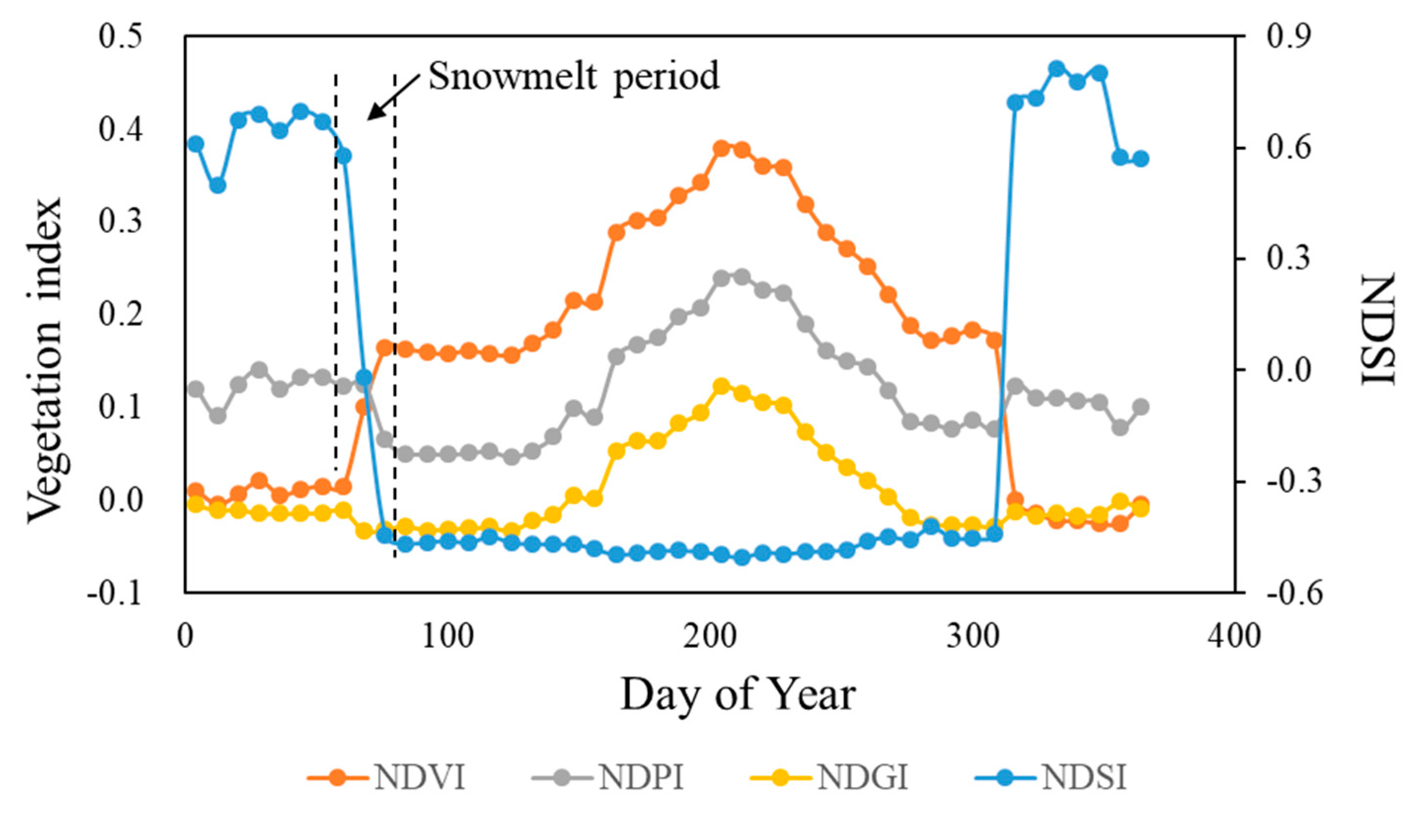
2.1. Definition of Snow-Free Vegetation Indices

We compared the performances of NDVI, NDPI, and NDGI for GUD detection. NDVI is calculated as the normalized form of red and NIR reflectance (${\rho }_R$ and ${\rho }_{NIR}$), expressed as:

$$\mathrm{NDVI}=\frac{{\rho }_{NIR}-{\rho }_R}{{\rho }_{NIR}+{\rho }_R }$$

(1)

NDPI incorporates red, NIR, and SWIR reflectance (${\rho }_R$, ${\rho }_{NIR}$, and ${\rho }_{SWIR}$, respectively) and is calculated as [22]:

$$\mathrm{NDPI}=\frac{{\rho }_{NIR}-\left[\alpha \times {\rho }_R+\left(1-\alpha \right)\times {\rho }_{SWIR}\right]}{{\rho }_{NIR}+\left[\alpha \times {\rho }_R+\left(1-\alpha \right)\times {\rho }_{SWIR}\right]}$$

(2)

where $\mathsf{\alpha }$is the weighted parameter that depends on the spectral configuration of satellite sensors.$\mathsf{\alpha }$is between 0.0 and 1.0 and was determined to be 0.74 for the MODIS (MODerate resolution Imaging Spectroradiometer) according to a data-driven experiment [22]. Actually, the spectral curve from the wavelength of red to NIR to SWIR monotonically decreases for snow, whereas increases for soil. Accordingly, NDPI makes use of this spectral change characteristic and employs the three bands to minimize the differences between soil and snow.

Yang et al. [23] argued that NDPI ignores the presence of dry vegetation in the background and developed the semi-analytical index NDGI. The general idea of NDGI is similar to that of NDPI (see Figure 1 in Yang et al., [23]), but NDGI uses the reflectance of green, red and NIR bands (${\rho }_G$, ${\rho }_R$, and ${\rho }_{NIR}$, respectively). NDGI is calculated as:

$$\mathrm{NDGI}=\frac{\alpha \times {\rho }_G+\left(1-\alpha \right)\times {\rho }_{NIR}-{\rho }_R}{\alpha \times {\rho }_G+\left(1-\alpha \right)\times {\rho }_{NIR}+{\rho }_R}$$

(3)

where $\alpha$is the weighted parameter depending on the spectral configuration of satellite sensor. $\alpha$was found to be 0.65 for MODIS data as suggested by Yang et al. [23].

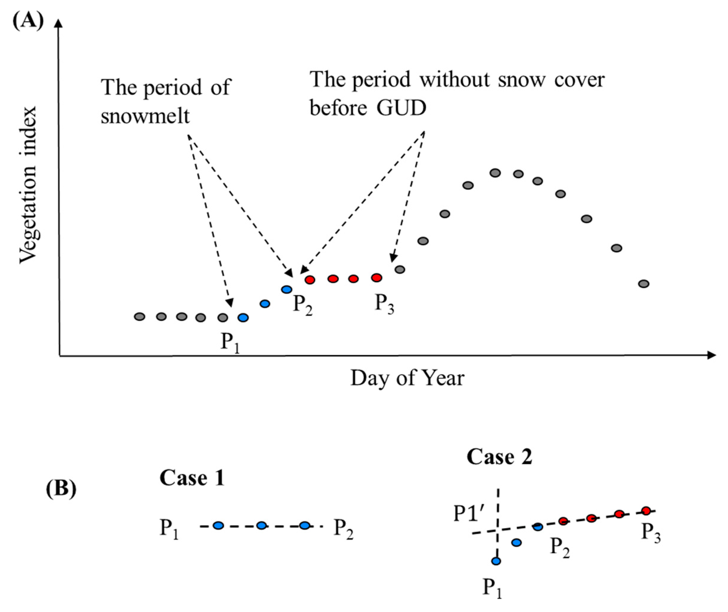
2.2. Detecting GUD from Vegetation Index (VI) Time-Series Data

We estimated GUD from VI time-series data by using the curvature method [1], which has been adopted to produce the MODIS land surface phenology product [28]. Specifically, we first used the four-parameter logistic function to fit VI time series during the rising period (i.e., from the start of a year to the date with the annual maximum VI). The logistic function form is shown as:

$$V{I}_{fit}\left(t\right)=\frac{c-d}{1+e^{a+bt}}+d$$

(4)

where t is the day of year (DOY), and$V{I}_{fit}\left(t\right)$ is the fitted VI value at the time t. The parameters d and c represent the background and maximum VI values of the logistic curve. Another two parameters a and b control the changes of the logistic curve from the background value to the maximum value. Based on the fitted curve, we calculated the curvature (K) of $V{I}_{fit}\left(t\right)$ as:

$$K=\frac{V{I}_{\mathrm{fit}}{\left(t\right)}^{″}}{{\left(1+{\left(V{I}_{\mathrm{fit}}{\left(t\right)}^{\prime }\right)}^2\right)}^{\frac{3}{2}}}$$

(5)

Therefore, GUD is defined at the date when the rate of change of the curve’s curvature (K) reaches its first local maximum [1].

2.3. Quantifying GUD Uncertainty Caused by Spring Snowmelt

To detect GUD from VI time-series data, it is necessary to determine the background VI (VI_BN) value (see Equation (4)). In the seasonally snow-covered areas, however, a reliable VI_BN may be difficult to be determined because VI (e.g., NDVI) may be greatly affected by the process of snowmelt before green-up. To this point, GUD uncertainty due to snowmelt is mainly caused by the determination on VI_BN. By considering the possible range of VI_BN, GUD uncertainty is thus defined as the difference of GUD estimations when using the upper and lower boundary values of VI_BN, which are graphically illustrated in detail in the following.

As the schematic shows in Figure 1A, the determination of VI_BN value is related to two key points P₁ and P₂, which represent the VI values at the start and end of snowmelt (expressed as VI(P₁) and VI(P₂)). The value of VI_BN can thus be firstly determined to be between VI(P₁) and VI(P₂). Further, vegetation growth from spring to summer is normally described by the logistic form (i.e., S-shaped curve); thus, VI time-series data exhibit an accelerating VI increase in the beginning [29]. It is reasonable to assume a more rapid increase in vegetation greenness in the period after the point P₂ than that in the period before P₂. By following this assumption, we can get the point $P_1^{\prime }$ (see case 2 in Figure 1B), which is defined as the linearly extrapolated VI value at the start of snowmelt. Here, the linear fitting employs the four points after the end of snowmelt for a robust fitting. In actuality, the point $P_1^{\prime }$ represents the VI value at the start of snowmelt when we consider that the change rate of VI before P₂ is identical to that after P₂. The value of VI_BN can then be determined to be between $VI\left({\mathrm{P}}_1^{\prime }\right)$and $VI\left(P_2\right)$. By comparing $\left[VI\left(P_1\right),VI\left(P_2\right)\right]$ with $\left[VI\left({\mathrm{P}}_1^{\prime }\right),VI\left(P_2\right)\right]$, the final range of VI_BN are determined to be the one with a smaller interval, expressed as:

$$V{I}_{\mathrm{BN}}=\{\begin{array}{c}\left[VI\left(P_1\right),VI\left(P_2\right)\right], \left|VI\left(P_1\right)-VI\left(P_2\right)\right|<\left|VI\left(\mathrm{P}{1}^{\prime }\right)-VI\left(P_2\right)\right|\\ \left[VI\left({\mathrm{P}}_1^{\prime }\right),VI\left(P_2\right)\right], \left|VI\left(P_1\right)-VI\left(P_2\right)\right|>\left|VI\left(\mathrm{P}{1}^{\prime }\right)-VI\left(P_2\right)\right|\end{array}$$

(6)

We use the lower and upper boundary values of VI_BN (Equation (6)) as the background VI to estimate GUD. For example, if VI_BN is determined to be within $\left[VI\left(P_1\right),VI\left(P_2\right)\right]$, the lower and upper boundary values are $VI\left(P_1\right)$ and $VI\left(P_2\right)$. Then, GUD uncertainty is calculated as the absolute difference of two GUD estimations with different background VI (i.e., $\left|GUD\left(VI\left(P_1\right)\right)-GUD\left(VI\left(P_2\right)\right)\right|$). Taking $GUD\left(VI\left(P_1\right)\right)$ as the example, we estimated $GUD\left(VI\left(P_1\right)\right)$ in three steps: (1) all VI values smaller than $VI\left(P_1\right)$ before the end of snowmelt were replaced by $VI\left(P_1\right)$; (2) the VI time-series data were smoothed by using 3-points median filter (MOD12Q1 User Guide); (3) GUD was detected by using Zhang’s curvature method (see Section 2.2).

According to the definition of GUD uncertainty, it is easy to understand that small GUD uncertainty can occur in two cases: (1) the VI value varies little during the period of snowmelt (i.e., the case 1 in Figure 1B); (2) the VI value varies little after the end of snowmelt, because in this case, the extrapolated $P_1^{\prime }$ is close to P₂ (i.e., the case 2 in Figure 1B). In other words, even if a VI is not snow-free (e.g., NDVI), GUD estimation from this VI can be less affected by snowmelt if there is a plateau with a stable VI value after the end of snowmelt. In some cases, snowmelt and GUD may occur concurrently. For these cases, the VI time-series data may increase continuously from the period of snowmelt, which could lead to large GUD uncertainty according to the definition of GUD uncertainty. The concurrent occurrence between snowmelt and GUD results in uncertainty for our analysis, which can be understood in two aspects. First, large GUD uncertainty for these cases is caused by the large variations in the determined background VI values, which is self-consistent with the definition of GUD uncertainty. Second, it is more likely that spring phenological characteristics observed in field (e.g., leaf unfolding) occurs during the period of snowmelt. However, satellite-derived GUD is defined at a date when land surface greenness reaches a threshold. For example, according to Zhang’s curvature method (i.e., Equation (5)) [1], GUD is defined at the date when greenness first reaches approximately 9.18% of vegetation growth amplitude [30]. Therefore, leaf unfolding may occur during the period of snowmelt but it may be more difficult for vegetation to reach the threshold of greenness that can be detected by satellite date.

To determine the period of snowmelt at each pixel, we employed the time series of normalized difference snow index (NDSI). NDSI employs the reflectance at MODIS band 4 (green band) and band 6 (a SWIR band), and calculated as the normalized form of the two bands (i.e., (band 4–band 6) / (band 4 + band 6)). It was found that NDSI is sensitive to the change of snow cover [27] and thus NDSI value dramatically decreases during snowmelt in spring (see an example in Figure 2 and more examples in Figure S1). Snowmelt was thus identified to be the period within which NDSI time-series data exhibits the largest decreasing slope. This identification mainly includes three steps: First, we smoothed the NDSI time series by using the 3-points median filter and performed linear fitting using the continuous consecutive 4 points. The use of 4 points (8-day temporal frequency for each point) is because snowmelt usually lasts 2–4 weeks [31,32]; Second, a preliminary period of snowmelt was determined to be the one with the lowest negative slope. The 4 points of this period can be expressed as Pi, Pi+1, Pi+2, and Pi+3; Third, we refined the preliminary period of snowmelt by further investigating edge points (i.e., Pi-1 and Pi at the left edge; Pi+3 and Pi+4 at the right edge). This step is employed to address some cases with a short period of snowmelt (e.g., a period of two points). Taking the point Pi-1 as an example, we calculated the difference between Pi-1 and its next point Pi (i.e., Pi-1- Pi) and defined that Pi-1 can be included into the snowmelt period if the difference was larger than the 10% of the range of NDSI value in the preliminary snowmelt period. Similar investigations were conducted for Pi, Pi+3, and Pi+4 to determine whether they are included into or excluded from the snowmelt period. We also noted that some methods have been developed to detect snow melt-off day based on optical or microwave radiometer data [33,34,35] and several snowmelt timing datasets have been released [36]. We did not adopt these methods and used the existing datasets because of two reasons. First, the existing snowmelt timing datasets [36] were not compatible with the spatial (0.05 degree) scale of this study. Second, the definition of snowmelt in previous methods is somewhat difficult to be applied in this study. For example, Metsämäki et al. [34] defined the melt-off day to be the first day of two weeks snow-free period by using fractional snow cover data, which is not a straightforward and intuitive way to measure the corresponding changes of both NDSI and various VIs during the period of snowmelt (Figure 2).

3. Experimental Design

3.1. Simulation Data and Experiments

We performed the simulation experiments in two simulation scenarios, which aims to investigate (1) whether NDGI improved GUD estimation compared with NDPI by considering the background component dry vegetation, and more importantly (2) whether it is consistent for the comparison results when using the uncertainty of GUD estimations or using the true error of GUD estimations. The simulations were based on the linear spectral mixture model [37], in which the reflectance of a pixel was simply modeled as the weighted sum of the reflectance of different components. By assuming that a pixel is comprised by green vegetation, soil, snow, and dry vegetation, the reflectance of this pixel is thus expressed as:

$${\rho }_{pixel}=f_v\times {\rho }_v+f_{soil}\times {\rho }_{soil}+f_{snow}\times {\rho }_{snow}+f_{dry}\times {\rho }_{dry},$$

(7)

where $f_v$, $f_{soil}$, $f_{snow}$, and $f_{dry}$ are the coverage for green vegetation, soil, snow, and dry vegetation, respectively, and their sum is 1.0.

Two scenarios were designed as follows. In scenario 1, without the component dry leaf, snowmelt starts at 60 day of year (DOY) and ends at 90 DOY with the snowmelt period of 30 days (Figure 3A). Green vegetation starts to grow during the snowmelt period (i.e., at 75 DOY). Therefore, the coverage of soil background initially increases with snowmelt and then gradually decreases with green vegetation growth (Figure 3A). It should be noted that the sum of the coverage of the three components is 1.0 at any time. In scenario 2, the change patterns of snow and green vegetation are set as the same as those in the scenario 1, but background components contain both soil and dry leaf (Figure 3B). For the two scenarios, vegetation growth starts at 75 DOY, but this definition is different from satellite-derived GUD defined in this study (i.e., Equation (5)). Therefore, we fitted the vegetation growth trajectory (i.e., the blue line in Figure 3) by the logistic function and determined GUD according to Zhang’s curvature method [1]. The true GUD was estimated to be at 108 DOY (the green line in Figure 3).

The reflectance spectra were selected from the Aster Spectral Library [38], including four types of green vegetation, three types of snow with different particle sizes, four types of dry leaf, and 25 types of soil (Figure 4). From these spectra we randomly picked out one spectrum from each component at a time to generate one time series (Equation (7)), which forms totally 300 time series (i.e., 4 $\times$ 3 $\times$ 25) for the scenario 1 and 1200 time series (i.e., 4 $\times$ 3 $\times$ 25 $\times$ 4) for the scenario 2. Here, the generated reflectance (Equation (7)) has been resampled by the spectral response functions of MODIS. For both scenarios, we detected GUD from different indices (NDVI, NDPI, and NDGI) by using Zhang’s curvature method [1]. To evaluate the performances of different indices, we estimated the true error of GUD estimation in each generated time series and also calculated the uncertainty of GUD estimation for different indices (see Section 2.3 for the definition of GUD uncertainty).

3.2. Satellite Data and Experiments

We collected the MODIS reflectance data product (Product No. MOD09A1) over northern middle and high latitudes (north of 40° N) during 2001–2016 from the website of the National Aeronautics and Space Administration (NASA) MOD09A1 has an 8-day temporal frequency and a 500-m spatial resolution. To reduce the huge computation load, the original reflectance data were first resampled to a spatial resolution of 0.05 degree by pixel aggregate and then were used to calculate NDVI, NDPI and NDGI according to Equations (1)–(3). We first filled some missing data in the VI time-series by a linear interpolation method and then applied the three-point median-value filter to the VI time-series data to remove outliers due to cloud or poor atmospheric conditions [28]. We estimated the uncertainty of GUD estimation from the three VIs during 2001–2016. To help understand their performances at the hemispheric scale, here we showed the land cover types from the MCD12C1 V6 product [39] for the year 2009 (i.e., the middle year of 2001–2016) (Figure 5). For the land cover types in 2001 and 2016, please refer to Figure S2 in the supplementary materials.

4. Results

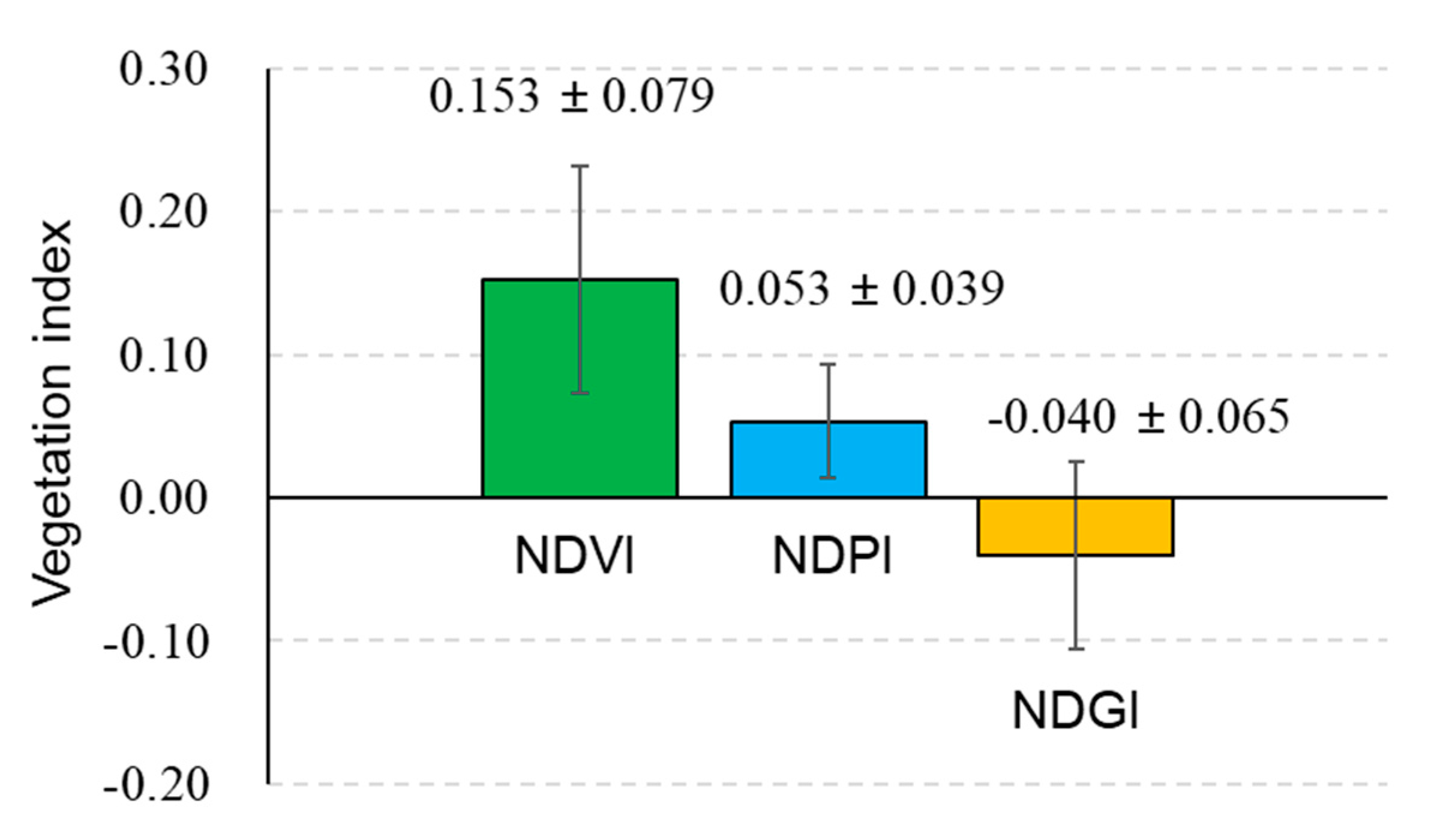
4.1. The Simulation Experiments

We quantified the GUD estimation error by calculating the Average Absolute Difference (AAD) between the estimated GUD and true GUD (108 DOY; Figure 3) (i.e.,$AAD=\left|GU{D}_{estimated}-GU{D}_{true}\right|$). As we expect, the results showed that compared with NDVI, NDPI and NDGI decreased GUD estimation errors for both simulation scenarios (Figure 6A), suggesting the usefulness of these snow-free vegetation indices for GUD detection. In scenario 1 in which there is no dry leaf, we found that NDPI performed better than NDGI with a lower mean value of AAD (the left panel in Figure 6A). However, NDGI achieved the best performance for GUD detection in scenario 2 with the presence of dry vegetation (the right panel in Figure 6A). These results highlight the uncertainty associate with applying these vegetation indices at global or regional scales, because which index is more appropriate for GUD detection depends on the background components in a given area.

We further investigated GUD uncertainty for both simulation scenarios (Figure 6B). We found that NDPI-based GUD has the smallest mean value of uncertainty in scenario 1 (snowmelt without dry leaf), whereas the smallest uncertainty value in scenario 2 (snowmelt with dry leaf) was found for NDGI-based GUD. Therefore, evaluations based on the defined uncertainty are generally consistent with those based on the true error (i.e., AAD), suggesting that GUD uncertainty can be used as an indirect way to evaluate the performance of NDVI, NDGI, and NDPI for GUD detection.

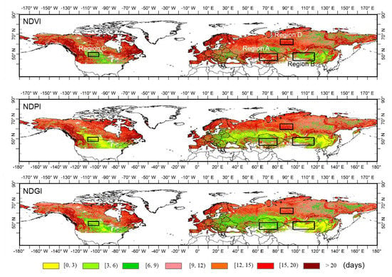
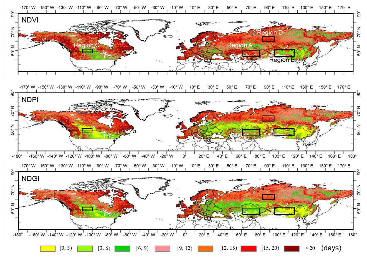
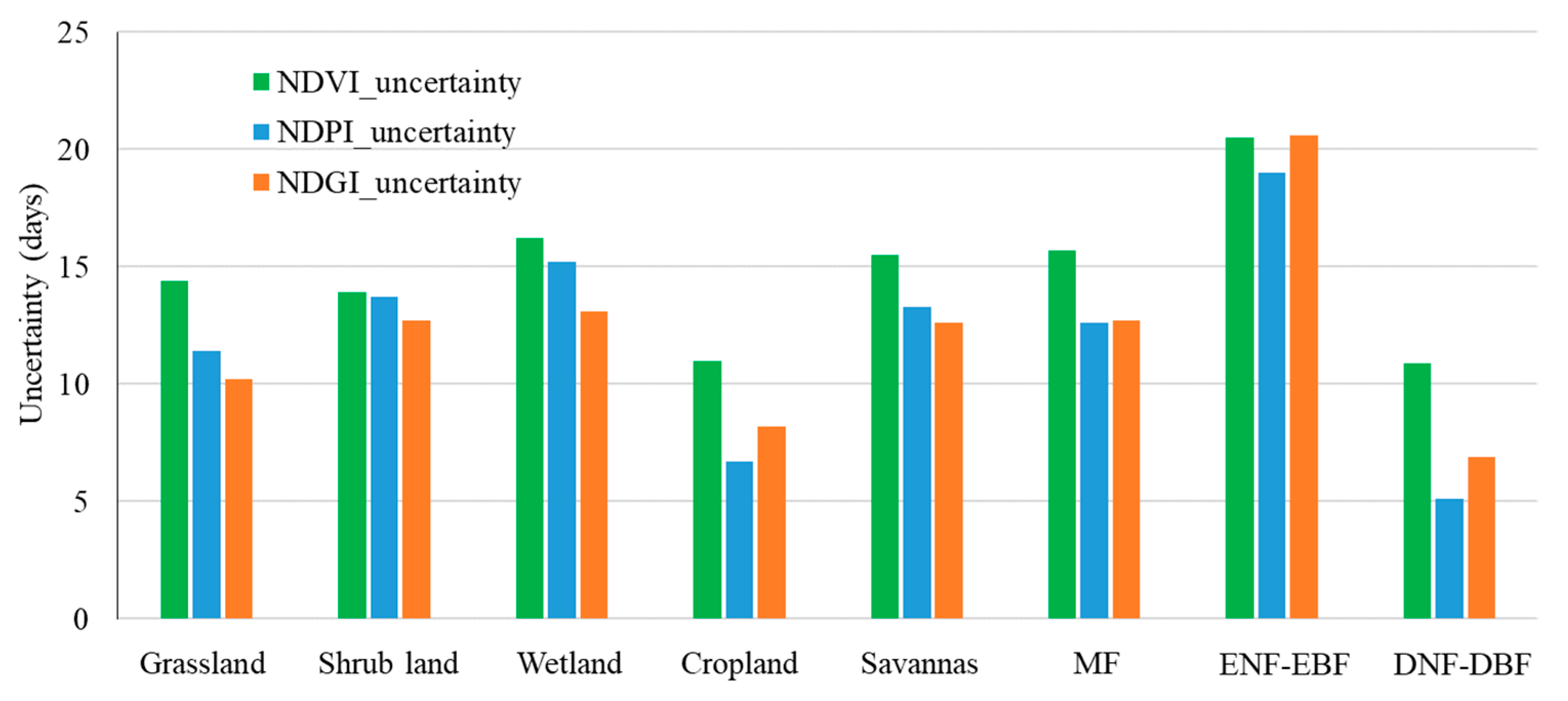
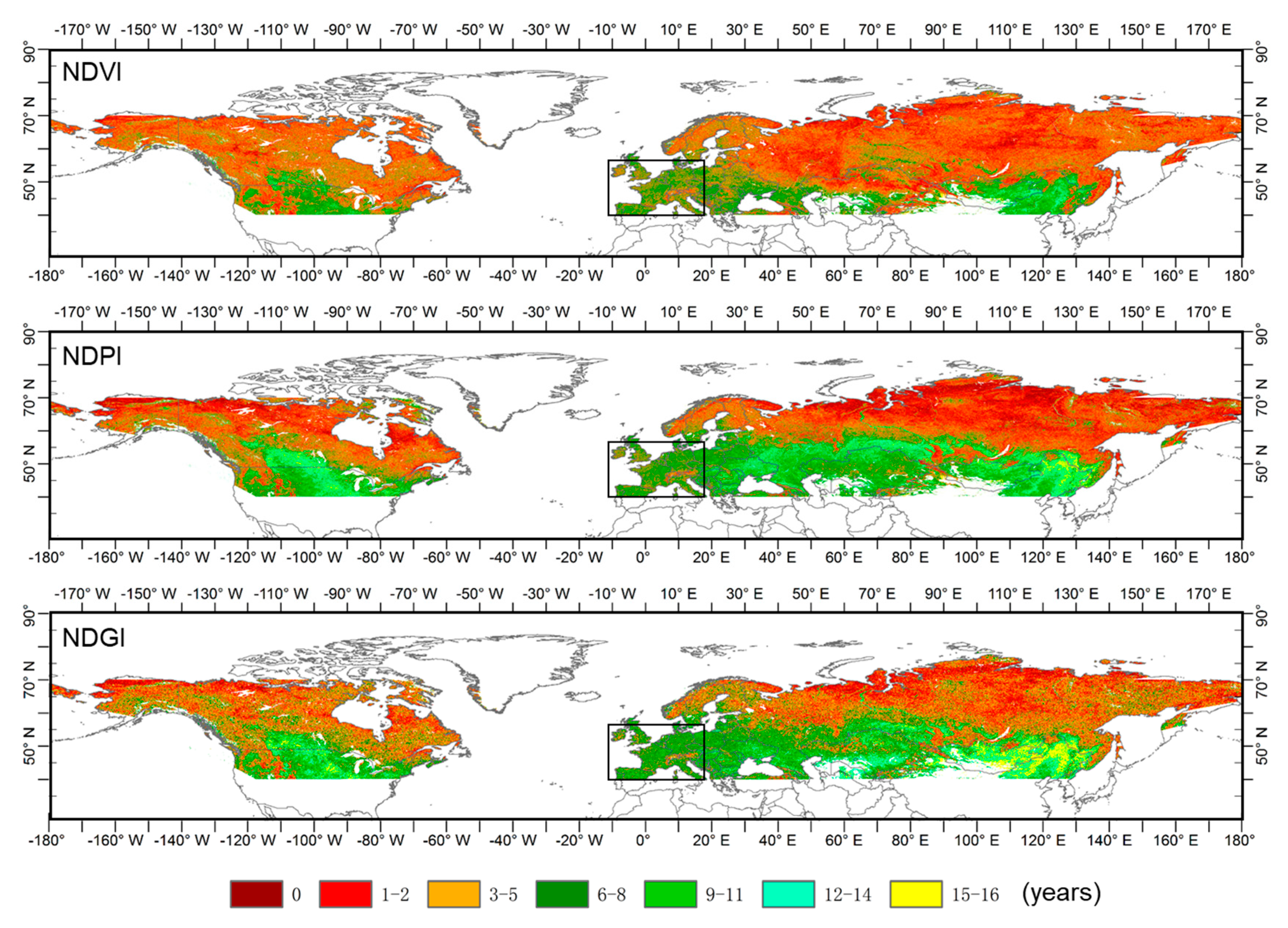
4.2. Comparisons of GUD Uncertainty at the Hemispheric Scale

Figure 7 shows the spatial distribution of GUD uncertainty averaged over 2001–2016 for the three vegetation indices. We found that in general, NDVI-based GUD had substantially larger uncertainty compared with the GUD estimations from NDPI and NDGI. NDVI only achieved satisfactory GUD estimations with the uncertainty smaller than 6 days in some local regions, such as the Mongolia grassland (i.e., Region B in Figure 7) and the central North America (i.e., Region C in Figure 7). In contrast, NDGI achieved good performance with small GUD uncertainty in the areas between 40° N and 55° N except western America and western Europe. Compared with NDGI, NDPI performs slightly better in the central North America (Region C) but worse in the grasslands of Kazakhstan (i.e., Region A in Figure 7). For the areas above approximately 55° N, all three indices exhibited large GUD uncertainty (e.g., Region D in Figure 7). These observations suggest that the snow-free indices NDPI and NDGI can be used for GUD detection below 55° N and the selection between NDPI and NDGI depends on the specific local regions.

To investigate the effect of vegetation types on GUD uncertainty, we further averaged the value of GUD uncertainty over all pixels within each vegetation type and compared the performances of NDVI, NDPI, and NDGI (Figure 8). We found that all three VIs performed well for deciduous forests, and NDPI performed especially well (5.1 days for GUD uncertainty). However, their performances became much worse when evergreens are dominant (e.g., evergreen forests and mixed forests). For grasslands, NDPI and NDGI performed better than NDVI and NDGI achieved the lowest value in GUD uncertainty.

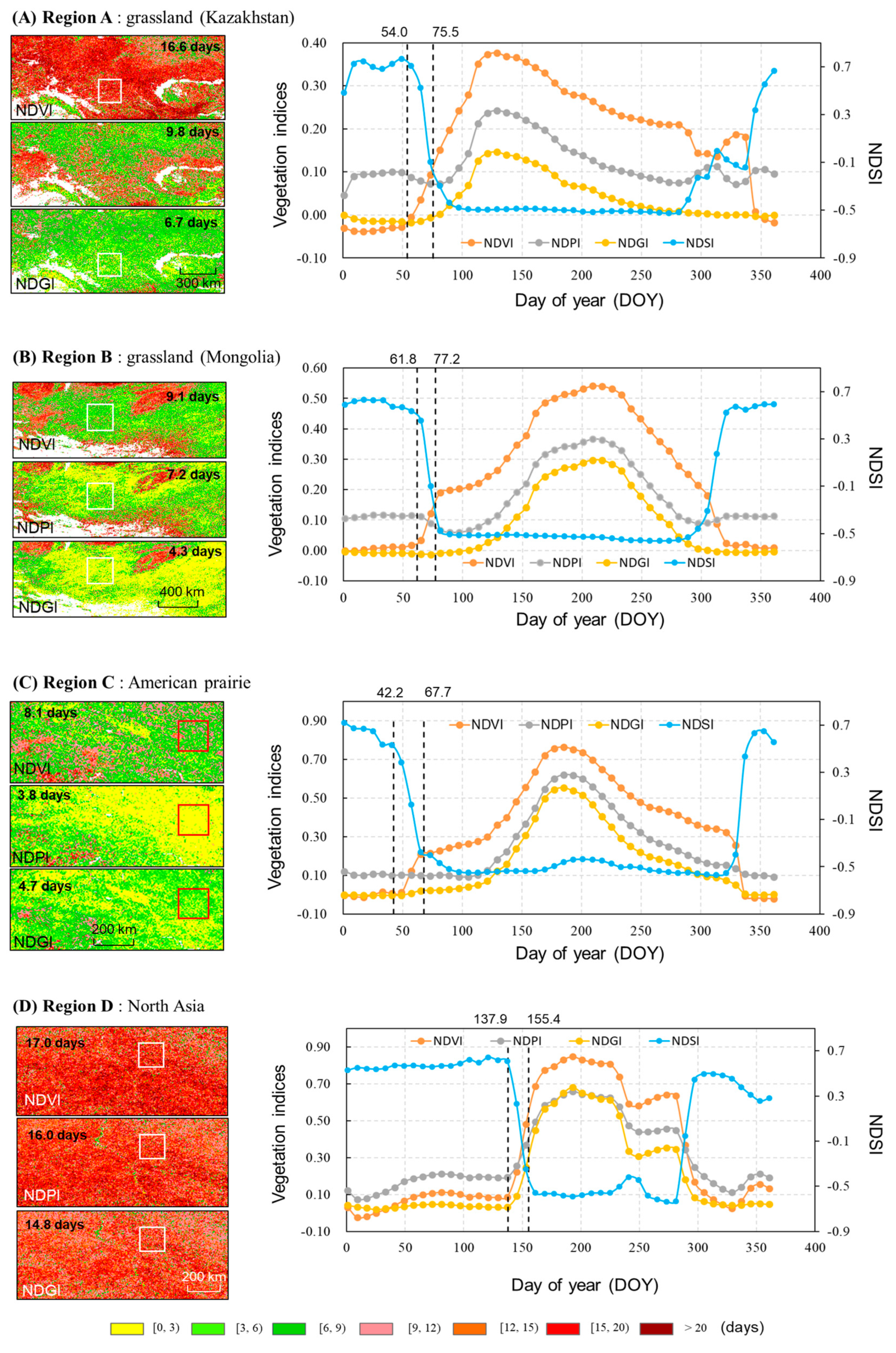
4.3. Comparisons between NDVI, NDPI, and NDGI in Some Local Regions

To explore the reasons of the different performances between indices, we further compared the time-series data of NDVI, NDPI, and NDGI in some local regions (Figure 9). The time-series data were generated by averaging all pixels within the white square in the left panels of Figure 9.

In the grassland of Kazakhstan (Region A), NDGI achieved the smallest GUD uncertainty (6.7 days) (Figure 9A). We found that the NDVI time series substantially increased during the period of snowmelt (54.0–75.5 DOY) and increased continuously after snowmelt. Therefore, it was difficult to decouple the process of snowmelt and vegetation growth because both processes increased NDVI, which led to a large uncertainty in NDVI-based GUD estimation. For the NDPI time-series data, NDPI decreased with snowmelt and then increased after snowmelt. The opposite effect that snowmelt decreased NDPI but vegetation growth increased NDPI accounted for the somewhat larger uncertainty of NDPI-based GUD estimations.

In the grassland of Mongolia (Region B), the performances of all three VIs seemed to be acceptable, although NDGI-based GUD still has the lowest uncertainty (Figure 9B). We found that in this region, NDVI time-series data increased during the period of snowmelt (61.8-77.2 DOY); however, a time period of about 1–2 months were observed between the end of snowmelt and GUD, which meant a stable NDVI background value could be determined. The small uncertainty of NDPI-based GUD in the Mongolian grassland can also be explained by this existing interval period.

In the American prairie (Region C), we found that GUD occurred about 1–2 months after the end of snowmelt; thus, the background values of the three VIs can be determined by the 4-points linear fitting (Figure 9C). It is more difficult to determine a reliable background value if the period between snowmelt and GUD is short with fluctuated VI values. In addition, the NDPI-based GUD estimations exhibited somewhat smaller uncertainty than the GUD estimations from NDGI in this region (i.e., 3.8 days vs. 4.7 days). In Northern Asia (Region D), where covered by evergreen or mix forests, all three VIs showed substantially larger GUD uncertainty (Figure 9D). We observed that both NDPI and NDGI increased during the period of snowmelt and unfortunately, both indices increased continuously after the end of snowmelt because in this region the date of the end of snowmelt is very late (about 155 DOY). This result highlights the difficulty of using vegetation greenness indices to detect GUD in the large areas of Northern Asia.

We counted the number of years with GUD uncertainty smaller than three days during 2001–2016 over the north of 40° N (Figure 9). We found that most of the areas below 55° N had the number of years more than six. An interesting phenomenon was observed in central and western Europe (the black box in Figure 9), where the average of GUD uncertainty during 2001–2016 in this region were almost larger than 15 days (see Figure 7) but more than six years had GUD uncertainty smaller than three days (see Figure 10). This phenomenon may be explained as follows: in central and western Europe, there are not always snowfalls in every year; thus, there are small GUD uncertainty in the years without snowfalls but large GUD uncertainty in other years with snowfalls. Because both NDPI and NDGI cannot reduce GUD uncertainty in this region, we hypothesize that large GUD uncertainty in the snowfall years is due to the exposure of evergreen components during snow melting. To test this hypothesis, we investigated the values of the three indices before GUD for the years with GUD uncertainty smaller than three days (Figure 11). Results showed that NDVI values before GUD were mainly above 0.4 in central and western Europe, confirming that there widely exist evergreen components before GUD in this region.

5. Discussion

Satellite-derived GUD has been widely used to investigate the response of terrestrial ecosystems to climate change [2,3,4,40]. Unfortunately, NDVI-based GUD are contaminated by snowmelt, which could lead to the misinterpretation of climate impact on GUD in the seasonally snow-covered regions such as the Tibetan Plateau [12,13,14] and northern Europe [15]. Recently, two promising vegetation indices NDPI and NDGI are proposed, both of which are called snow-free index and are designed to address the snowmelt effect on phenological detection. To popularize their practical applications, we conducted detailed comparisons between NDVI, NDPI, and NDGI for GUD detection at the hemispheric scale. Three findings are summarized.

First, compared with NDVI, NDPI and NDGI indeed improve the accuracy of GUD detection, but the improvement is mainly acquired in the areas below 55° N (Figure 7). In the high-latitude areas (55° N-70°N), all three VIs show large GUD uncertainty. This obvious latitude-dependent spatial pattern of GUD uncertainty may be explained by two factors. First, the end of snowmelt seems to be later with the increase of latitude. For example, the end of snowmelt occurs in late March in the areas around 50° N (e.g., see the points 3, 4, 5, and 9 in Figure S1) and in late May in the areas around 60° N (e.g., see the points 1, 2, and 10 in Figure S1). Due to the very late snowmelt date in the high-latitude areas, a stable VI background value cannot be easily found in this region. Second, in the high-latitude areas, we found that all three VIs increase continuously during the period of snowmelt (Figure 9D). The increase in all VIs values may be caused by the exposure of evergreen component during the period of snowmelt. In addition, the start of vegetative growth may occur in the period of snowmelt in the high latitudes. In these areas, solar radiation hits the snow surface at a small solar elevation angle, which causes less energy transfer to the snowpack and slower snowmelt. In contrast, any vegetation that does emerge from the snow (e.g., spruce trees) can intercept that solar energy orthogonal to the incoming solar radiation, allowing for vegetative productivity prior to snowmelt. Many previous studies detected GUD from the traditional vegetation greenness indices (e.g., NDVI) and investigated climate impact on GUD in the northern high-latitude areas. To remove snow on NDVI time-series data, they usually employed a predefined NDVI background value to replace the snow-contaminated winter NDVI values [40,41]. Here, we would like to emphasize that our current results do not necessarily mean that these previous GUD estimations have larger errors, but imply large uncertainty of these GUD estimations due to possible background VIs values. To estimate GUD in the northern high-latitude areas, two novel alternatives to vegetation greenness indices may be the photochemical reflectance index (PRI) [42,43] and the solar-induced vegetation chlorophyll fluorescence [44]. However, it must keep in mind that GUD estimated from PRI and fluorescence is related to the initial increase of photosynthetic efficiency, which has different ecological meanings compared with GUD estimated from vegetation greenness indices.

The second finding is that the selection between NDVI, NDPI, and NDGI in the areas below 55° N depends on vegetation types in local regions. We found that NDGI-based GUD estimations were stable and reliable in the arid and semi-arid grasslands, such as Mongolia and Central Asia (e.g., Kazakhstan), whereas NDPI performed not so satisfactory in these regions (Figure 9). Our results at the regional scale are probably explained by the ability of NDGI to account for dry vegetation as suggested by Yang et al. [23], because dry vegetation is a common component on the soil background in the arid and semi-arid grasslands [45]. In addition to the composition of background, GUD uncertainty is also affected by the interval period between the end of snowmelt and GUD. For example, vegetation green up occurs more than one month after the end of snowmelt in Mongolia; thus, even NDVI-based GUD are found to be roughly acceptable in this region.

In the American prairie, we found slightly better performances of NDPI (Figure 9C). The higher accuracy of NDPI-based GUD was also observed in our simulation experiments in scenario 1 (without dry leaf), which may be because NDPI better accounts for the variations in soil spectra. Here, we further investigated the variations of NDVI, NDPI, and NDGI for 4438 soil types. The large amount of soil types was collected from the Soil Information System (ISIS) of the International Soil Reference and Information Centre (ISRIC) [46]. We first employed the spectral response function of MODIS to resample all the soil spectra and we then calculated the NDVI, NDPI, and NDGI values for all the soil spectra. We found that the standard deviation (SD) of NDVI, NDPI, and NDGI for all soil types is 0.079, 0.039, 0.065, respectively (Figure 12), suggesting that NDPI can suppresses the variations in soil background best. Chen et al. [47] also found that using the Red-SWIR band to replace the Red band, the formula form adopted by NDPI, can greatly reduce the variations in soil background. The better ability of suppressing the variations in soil background may partly account for the better performance of NDPI in the regions without serious mixture of soil and dry vegetation. However, the explanations need further field investigations and measurements in the future.

Third, we found large GUD uncertainty in central and western Europe. Snowfall does not occur regularly every year in this region, which leads to reliable GUD in the years where snow does not contaminate the VI signal. We further investigated the background VI values in the years without snowfall but found that these background values vary a lot between years (data not shown), which suggest that it is impossible to determine a stable and yearly invariable background VI value. Nevertheless, using GUD estimations from the years without snowfall may be a way to investigate the temporal shift and spatial distribution of GUD across middle and northern Europe.

For the applications of NDPI and NDGI, $\alpha$ is a key parameter (see Equations (2) and (3)) which determines whether the variance of background VI values can be suppressed. $\alpha$ depends on the spectral configuration of satellite sensor. Here, we performed an additional experiment to investigate how $\alpha$ affects the VI value of vegetation and the variance of background VI values for both MODIS and its next generation sensor VIIRS (Visible/Infrared Imager/Radiometer Suit) onboard the S-NPP satellite [48]. A $\alpha$ value is expected to be a better one if the variance of background VI values is smaller and the VI value for vegetation is larger. In this experiment, we employed the endmember spectra as those used in Figure 4 (i.e., 4 green vegetation spectra, 3 snow spectra, 4 dry leaves spectra, and 25 soil spectra). We changed $\alpha$ from 0 to 1 at a step of 0.01, and at each $\alpha$ value we calculated the NDPI and NDGI values for the 4 green vegetation spectra and the variance of NDPI and NDGI for the 32 background spectra (i.e., 3+4+25=32). All spectra have been resampled by the spectral response functions of MODIS and VIIRS, respectively. Results show that vegetation NDPI increases by increasing $\alpha$, whereas the variance of background NDPI values exhibits the smallest when $\alpha$ is approximately 0.73–0.74 (Figure 13), suggesting that the value of 0.74 for $\alpha$ in NDPI as adopted by Wang et al. [22] is acceptable for both MODIS and VIIRS. For NDGI, Yang et al. [23] recommended the value of 0.65 for $\alpha$. Our investigations supported this $\alpha$ value and confirmed that it can be applied for VIIRS NDGI. Further, the nearly identical curves between MODIS (upper panels in Figure 13) and VIIRS (lower panels in Figure 13) highlight that the detailed comparisons between MODIS NDPI and NDGI in this study can also provide guidelines for the applications of VIIRS NDPI and NDGI to detect GUD in seasonal snow-covered areas.

We recognized that current analyses still have some limitations. First, there is more likely large GUD uncertainty for a vegetation index that is more sensitive to early vegetation greenup, because it may be more difficult for this index to determine a stable background VI from the period between P₂ and P₃ (Figure 1). We expect that the sensitivities of NDVI, NDPI, and NDGI to vegetation greenup are similar because the three VIs have similar formula forms (normalized ratio form) and they all quantify the spectral changes of green vegetation from the wavelength of red to NIR. Wang et al. [22] and Yang et al. [23] tested NDVI, NDPI and NDGI at a number of flux sites and phenological camera sites and did not observe different sensitivity to vegetation greenup between the three VIs. Second, in addition to snowmelt, the accuracy of GUD estimations from VIs time-series data is also affected by several other factors, such as the deviation of VIs time-series data from the ideal S-shaped curve under unsatisfactory vegetation growth conditions [49]. The coupling effect of snowmelt and other factors on GUD estimation may be an error source in our results. Third, we did not compare GUD estimations with ground phenological observations because previous studies have conducted such comparisons at some field sites [18,22,23]. In this study, we investigated GUD uncertainty caused by snowmelt for NDVI, NDPI, and NDGI. Such investigations may be the only way to perform the detailed comparisons at the hemispheric scale. In the future study, however, it is necessary to conduct some field measurements and experiments in the areas as we particularly pointed out. Fourth, we determined the period of snowmelt from NDSI time-series data and detected GUD from the VIs time-series data. The NDSI and VIs time-series data may be contaminated by cloud. We smoothed these time-series data by using the three-point median-value filter, which has been also adopted in the generation of MODIS phenology product (MCD12Q2). Compared with some other smoothing filters (e.g., the Asymmetric Gaussian filter), the three-point median-value filter has the advantage to better preserve the phenological characteristics in the VIs time-series data [50]. However, the time-series data smoothed by this filter may not be so good for the areas where continuous cloud contamination is serious and vegetation annual growth curve is complex. Fifth, in this study, the investigations were performed at a spatial resolution of 0.05 degree. The performances of the three VIs may be affected by the spatial resolution in some heterogeneous areas where there are different vegetation types within a pixel [51]. For example, for mixed forests at northern high latitudes, smaller GUD uncertainty may be found for some pixels at finer spatial resolution if these finer pixels are mainly composed by deciduous forests and thus are less affected by the exposure of evergreen component during the period of snowmelt. In addition, in some mountain areas, different periods of snowmelt may exist within a coarser pixel because of large variations in altitude within a coarse pixel. The Qinghai-Tibetan Plateau may be a typical area to investigate such phenomenon. This study investigated GUD uncertainty at northern middle and high latitudes. In the future study, we can further focus on GUD detection in the high-altitude areas, such as the Qinghai-Tibetan Plateau where great temporal shift in GUD has been reported [12,52].

6. Conclusions

Spring snowmelt affects GUD estimations in seasonally snow-covered areas. NDPI and NDGI, two snow-free VIs, have been developed for GUD detection but detailed evaluations on their performances at the large spatial scale is still lacking. In this study, we compared the performances between NDPI, NDGI, and NDVI for GUD detection at northern middle and high latitudes (north of 40° N). We estimated GUD from the three VIs time-series data and quantified snowmelt-induced uncertainty of GUD estimations by considering the changes in VI values caused by snowmelt. We found an obvious latitude-dependent spatial pattern of GUD uncertainty. In the areas between 40° N and 55° N, NDPI and NDGI achieved much lower GUD uncertainty than NDVI, whereas in the high-latitude areas (55° N-70°N), all three VIs exhibited large GUD uncertainty. Furthermore, we found differences in the performances of the three VIs for different vegetation types. All three VIs performed much better for deciduous forests, and NDPI performed especially well (5.1 days for GUD uncertainty). In the arid and semi-arid grasslands, NDGI-based GUD estimations are more reliable than NDPI-based GUD (e.g., GUD uncertainty for NDGI vs. NDPI: 4.3 d vs. 7.2 d in Mongolia grassland and 6.7 d vs. 9.8 d in Central Asia grassland). In American prairie, NDPI-based GUD estimations are slightly better than NDGI-based GUD estimations (GUD uncertainty for NDPI vs. NDGI is 3.8 d vs. 4.7 d). The performances of all three VIs became much worse when evergreens are dominant (e.g., evergreen forests and mixed forests). This study elucidates the differences between NDVI, NDPI, and NDGI to allow for more precise applications of these VIs in seasonally snow-covered areas.

References

1. Zhang, X.; Friedl, M.A.; Schaaf, C.B.; Strahler, A.H.; Hodges, J.C.F.; Gao, F.; Reed, B.C.; Huete, A. Monitoring vegetation phenology using MODIS. Remote Sens. Environ. 2003, 84, 471–475. [Google Scholar] [CrossRef]
2. Pettorelli, N.; Vik, J.O.; Mysterud, A.; Gaillard, J.-M.; Tucker, C.J.; Stenseth, N.C. Using the satellite-derived NDVI to assess ecological responses to environmental change. Trends Ecol. Evol. 2005, 20, 503–510. [Google Scholar] [CrossRef] [PubMed]
3. White, M.A.; Hoffman, F.; Hargrove, W.W.; Nemani, R.R. A global framework for monitoring phenological responses to climate change. Geophys. Res. Lett. 2005, 32. [Google Scholar] [CrossRef] [Green Version]
4. Wolkovich, E.M.; Cook, B.; Allen, J.; Crimmins, T.; Betancourt, J.; Travers, S. Warming experiments underpredict plant phenological responses to climate change. Nature 2012, 485, 494–497. [Google Scholar] [CrossRef] [PubMed]
5. Rouse, J.W.; Haas, R.H.; Scheel, J.A.; Deering, D.W. Monitoring Vegetation Systems in the Great Plains with ERTS. In Proceedings of the 3rd Earth Resource Technology Satellite (ERTS) Symposium 1, College Station, TX, USA, 1 January 1974; pp. 48–62. [Google Scholar]
6. Tucker, C.J. Red and photographic infrared linear combinations for monitoring vegetation. Remote Sens. Environ. 1979, 8, 127–150. [Google Scholar] [CrossRef] [Green Version]
7. Asam, S.; Callegari, M.; Matiu, M.; Fiore, G.; De Gregorio, L.; Jacob, A.; Menzel, A.; Zebisch, M.; Notarnicola, C. Relationship between Spatiotemporal Variations of Climate, Snow Cover and Plant Phenology over the Alps—An Earth Observation-Based Analysis. Remote Sens. 2018, 10, 1757. [Google Scholar] [CrossRef] [Green Version]
8. Liu, L.; Cao, R.; Shen, M.; Chen, J.; Wang, J.; Zhang, X. How Does Scale Effect Influence Spring Vegetation Phenology Estimated from Satellite-Derived Vegetation Indexes? Remote Sens. 2019, 11, 2137. [Google Scholar] [CrossRef] [Green Version]
9. Wardlow, B.D.; Kastens, J.H.; Egbert, S.L. Using USDA Crop Progress Data for the Evaluation of Greenup Onset Date Calculated from MODIS 250-Meter Data. Photogramm. Eng. Remote Sens. 2006, 72, 1225–1234. [Google Scholar] [CrossRef] [Green Version]
10. Boschetti, M.; Stroppiana, D.; Brivio, P.A.; Bocchi, S. Multi-year monitoring of rice crop phenology through time series analysis of MODIS images. Int. J. Remote Sens. 2009, 30, 4643–4662. [Google Scholar] [CrossRef]
11. Ma, X.; Huete, A.; Tran, N.N. Interaction of Seasonal Sun-Angle and Savanna Phenology Observed and Modelled using MODIS. Remote Sens. 2019, 11, 1398. [Google Scholar] [CrossRef] [Green Version]
12. Shen, M.G.; Zhang, G.X.; Cong, N.; Wang, S.P.; Kong, W.D.; Piao, S.L. Increasing altitudinal gradient of spring vegetation phenology during the last decade on the Qinghai–Tibetan Plateau. Agric. For. Meteorol. 2014, 189–190, 71–80. [Google Scholar] [CrossRef]
13. Shen, M.G.; Sun, Z.; Wang, S.; Zhang, G.; Kong, W.; Chen, A.; Piao, S. No evidence of continuously advanced green-up dates in the Tibetan Plateau over the last decade. Proc. Natl. Acad. Sci. USA 2013, 110, E2329. [Google Scholar] [CrossRef] [PubMed] [Green Version]
14. Wang, T.; Peng, S.; Lin, X.; Chang, J. Declining snow cover may affect spring phenological trend on the Tibetan Plateau. Proc. Natl. Acad. Sci. USA 2013, 110, E2854–E2855. [Google Scholar] [CrossRef] [PubMed] [Green Version]
15. Jin, H.X.; Jönsson, A.M.; Bolmgren, K.; Langvall, O.; Eklundh, L. Disentangling remotely-sensed plant phenology and snow seasonality at northern Europe using MODIS and the plant phenology index. Remote Sens. Environ. 2017, 198, 203–212. [Google Scholar] [CrossRef]
16. Delbart, N.; Kergoat, L.; Le Toan, T.; Lhermitte, J.; Picard, G. Determination of phenological dates in boreal regions using normalized difference water index. Remote Sens. Environ. 2005, 97, 26–38. [Google Scholar] [CrossRef] [Green Version]
17. Shabanov, N.V.; Zhou, L.; Knyazikhin, Y.; Myneni, R.B.; Tucker, C.J. Analysis of interannual changes in northern vegetation activity observed in AVHRR data from 1981 to 1994. IEEE Trans. Geosci. Remote Sens. 2002, 40, 115–130. [Google Scholar] [CrossRef] [Green Version]
18. Gonsamo, A.; Chen, J.M.; Price, D.T.; Kurz, W.A.; Wu, C. Land surface phenology from optical satellite measurement and CO2 eddy covariance technique. J. Geophys. Res. Biogeosci. 2012, 117. [Google Scholar] [CrossRef]
19. Delbart, N.; Le Toan, T.; Kergoat, L.; Fedotova, V. Remote sensing of spring phenology in boreal regions: A free of snow-effect method using NOAA-AVHRR and SPOTVGT data (1982–2004). Remote Sens. Environ. 2016, 101, 52–62. [Google Scholar] [CrossRef]
20. Dunn, A.H.; de Beurs, K.M. Land surface phenology of North American mountain environments using moderate resolution imaging spectroradiometer data. Remote Sens. Environ. 2011, 115, 1220–1233. [Google Scholar] [CrossRef]
21. Peckham, S.D.; Ahl, D.E.; Serbin, S.P.; Gower, S.T. Fire-induced changes in green-up and leaf maturity of the Canadian boreal forest. Remote Sens. Environ. 2008, 112, 3594–3603. [Google Scholar] [CrossRef]
22. Wang, C.; Chen, J.; Wu, J.; Tang, Y.; Shi, P.; Black, T.A.; Zhu, K. A snow-free vegetation index for improved monitoring of vegetation spring green-up date in deciduous ecosystems. Remote Sens. Environ. 2017, 196, 1–12. [Google Scholar] [CrossRef]
23. Yang, W.; Kobayashi, H.; Wang, C.; Shen, M.G.; Chen, J.; Matsushita, B.; Tang, Y.H.; Kim, Y.W.; Bret-Harte, S.; Zona, D.; et al. A semi-analytical snow-free vegetation index for improving estimation of plant phenology in tundra and grassland ecosystems. Remote Sens. Environ. 2019, 228, 31–44. [Google Scholar] [CrossRef]
24. Jiang, Z.; Huete, A.R.; Didan, K.; Miura, T. Development of a two-band enhanced vegetation index without a blue band. Remote Sens. Environ. 2008, 112, 3833–3845. [Google Scholar] [CrossRef]
25. Jin, H.X.; Eklundh, L. A physically based vegetation index for improved monitoring of plant phenology. Remote Sens. Environ. 2014, 152, 512–525. [Google Scholar] [CrossRef]
26. Todd, S.W.; Hoffer, R.M. Responses of spectral indices to variations in vegetation cover and soil background. Photogramm. Eng. Remote Sens. 1998, 64, 915–922. [Google Scholar]
27. Hall, D.K.; Riggs, G.A.; Salomonson, V.V.; DiGirolamo, N.E.; Bayr, K.J. MODIS snow-cover products. Remote Sens. Environ. 2002, 83, 181–194. [Google Scholar] [CrossRef] [Green Version]
28. Ganguly, S.; Friedl, M.A.; Tan, B.; Zhang, X.; Verma, M. Land surface phenology from MODIS: Characterization of the Collection 5 global land cover dynamics product. Remote Sens. Environ. 2010, 114, 1805–1816. [Google Scholar] [CrossRef] [Green Version]
29. Wang, C.; Chen, J.; Tang, Y.H.; Black, T.A.; Zhu, K. A Novel Method for Removing Snow Melting-Induced Fluctuation in GIMMS NDVI3g Data for Vegetation Phenology Monitoring: A Case Study in Deciduous Forests of North America. IEEE J. Sel. Top. Appl. Earth Obs. Remote Sens. 2018, 11, 800–807. [Google Scholar] [CrossRef]
30. Shang, R.; Liu, R.; Xu, M.; Liu, Y.; Zuo, L.; Ge, Q. The relationship between threshold-based and inflexion-based approaches for extraction of land surface phenology. Remote Sens. Environ. 2017, 199, 167–170. [Google Scholar] [CrossRef]
31. Blume-Werry, G.; Jansson, R.; Milbau, A. Root phenology unresponsive to earlier snowmelt despite advanced above-ground phenology in two subarctic plant communities. Funct. Ecol. 2007, 31, 1493–1502. [Google Scholar] [CrossRef]
32. Winchell, T. Early snowmelt decreases ablation period carbon uptake in a high elevation, subalpine forest, Niwot Ridge, Colorado, USA. In Proceedings of the AGU Fall Meeting, San Francisco, CA, USA, 5–9 December 2019. [Google Scholar]
33. Berman, E.E.; Bolton, D.K.; Coops, N.C.; Mityok, Z.K.; Stenhouse, G.B.; Moore, R.D. Daily estimates of Landsat fractional snow cover driven by MODIS and dynamic time-warping. Remote Sens. Environ. 2018, 216, 635–646. [Google Scholar] [CrossRef]
34. Metsämäki, S.; Böttcher, K.; Pulliainen, J.; Luojus, K.; Cohen, J.; Takala, M.; Mattila, O.; Schwaizer, G.; Derksen, C.; Koponen, S. The accuracy of snow melt-off day derived from optical and microwave radiometer data-A study for Europe. Remote Sens. Environ. 2018, 211, 1–12. [Google Scholar] [CrossRef]
35. O’Leary, D.; Hall, D.; Medler, M.; Flower, A. Quantifying the early snowmelt event of 2015 in the Cascade Mountains, USA by developing and validating MODIS-based snowmelt timing maps. Front. Earth Sci. 2018, 693–710. [Google Scholar] [CrossRef]
36. O’Leary, D.; Hall, D.K.; Medler, M.; Matthews, R.; Flower, A. Snowmelt Timing Maps Derived from MODIS for North America, 2001–2015. Oak Ridge Natl. Lab. 2017. [Google Scholar] [CrossRef]
37. Adams, J.B.; Smith, M.O.; Johnson, P.E. Spectral mixture modeling: A new analysis of rock and soil types at the Viking Lander 1 site. J. Geophys. Res. Solid Earth. 1986, 91, 8098–8112. [Google Scholar] [CrossRef]
38. Baldridge, A.M.; Hook, S.J.; Grove, C.I.; Rivera, G.G. The ASTER spectral library version 2.0. Remote Sens. Environ. 2009, 113, 711–715. [Google Scholar] [CrossRef]
39. Sulla-Menashe, D.; Gray, J.M.; Abercrombie, S.P.; Friedl, M.A. Hierarchical mapping of annual global land cover 2001 to present: The MODIS Collection 6 Land Cover product. Remote Sens. Environ. 2019, 222, 183–194. [Google Scholar] [CrossRef]
40. Wang, C.; Cao, R.; Chen, J.; Rao, Y.; Tang, Y. Temperature sensitivity of spring vegetation phenology correlates to within-spring warming speed over the Northern Hemisphere. Ecol. Indic. 2015, 50, 62–68. [Google Scholar] [CrossRef]
41. Cao, R.Y.; Chen, Y.; Shen, M.G.; Chen, J.; Zhou, J.; Wang, C.; Yang, W. A simple method to improve the quality of NDVI time-series data by integrating spatiotemporal information with the Savitzky-Golay filter. Remote Sens. Environ. 2018, 217, 244–257. [Google Scholar] [CrossRef]
42. Gamon, J.; Penuelas, J.; Field, C. A narrow-waveband spectral index that tracks diurnal changes in photosynthetic efficiency. Remote Sens. Environ. 1992, 41, 35–44. [Google Scholar] [CrossRef]
43. Ulsig, L.; Nichol, C.J.; Huemmrich, K.F.; Landis, D.R.; Middleton, E.M.; Lyapustin, A.I.; Mammarella, I.; Levula, J.; Porcar-Castell, A. Detecting Inter-Annual Variations in the Phenology of Evergreen Conifers Using Long-Term MODIS Vegetation Index Time Series. Remote Sens. 2017, 9, 49. [Google Scholar] [CrossRef] [Green Version]
44. Chang, Q.; Xiao, X.M.; Jiao, W.Z.; Wu, X.C.; Doughty, R.; Wang, J.; Du, L.; Zou, Z.H.; Qin, Y.W. Assessing consistency of spring phenology of snow-covered forests as estimated by vegetation indices, gross primary production, and solar-induced chlorophyll fluorescence. Agric. For. Meteorol. 2019, 275, 305–316. [Google Scholar] [CrossRef]
45. Cao, X.; Chen, J.; Matsushita, B.; Imura, H. Developing a MODIS-based index to discriminate dead fuel from photosynthetic vegetation and soil background in the Asian steppe area. Int. J. Remote Sens. 2010, 31, 1589–1604. [Google Scholar] [CrossRef]
46. Garrity, D.; Bindraban, P. A Globally Distributed Soil Spectral Library Visible near Infrared Diffuse Reflectance Spectra; Soil-Plant Spectral Diagnostics Laboratory: Nairobi, Kenya, 2004. [Google Scholar]
47. Chen, X.H.; Guo, Z.F.; Chen, J.; Yang, W.; Yao, Y.M.; Zhang, C.S.; Cui, X.H.; Cao, X. Replacing the Red Band with the Red-SWIR Band (0.74ρred+0.26ρswir) Can Reduce the Sensitivity of Vegetation Indices to Soil Background. Remote Sens. 2019, 11, 851. [Google Scholar] [CrossRef] [Green Version]
48. Vargas, M.; Miura, T.; Shabanov, N.; Kato, A. An initial assessment of Suomi NPP VIIRS vegetation index EDR. J. Geophys. Res. Atmos. 2019, 118, 12301–12316. [Google Scholar] [CrossRef] [Green Version]
49. Cao, R.Y.; Chen, J.; Shen, M.G.; Tang, Y.H. An improved logistic method for detecting spring vegetation phenology in grasslands from MODIS EVI time-series data. Agric. For. Meteorol. 2015, 200, 9–20. [Google Scholar] [CrossRef]
50. Zhang, X.; Friedl, M.A.; Schaaf, C.B. Global vegetation phenology from Moderate Resolution Imaging Spectroradiometer (MODIS): Evaluation of global patterns and comparison with in situ measurements. J. Geophys. Res. Biogeosci. 2006, 111. [Google Scholar] [CrossRef]
51. Chen, X.; Wang, D.; Chen, J.; Wang, C.; Shen, M. The mixed pixel effect in land surface phenology: A simulation study. Remote Sens. Environ. 2018, 211, 338–344. [Google Scholar] [CrossRef]
52. Cao, R.Y.; Shen, M.G.; Zhou, J.; Chen, J. Modeling vegetation green-up dates across the Tibetan Plateau by including both seasonal and daily temperature and precipitation. Agric. For. Meteorol. 2018, 249, 176–186. [Google Scholar] [CrossRef]
Figure 1. (A) A schematic showing the relationship between the background value of a vegetation index and two periods (P1P2 and P2P3); (B) enlarged view of the two periods. Case 1 represents the period of snowmelt and case 2 represents a period after snowmelt.
Remotesensing 12 00190 g001
Figure 2. An example showing an annual time series of normalized difference vegetation index (NDVI), normalized difference phenology index (NDPI), and Normalized Difference Snow Index (NDSI). NDSI was found to dramatically decrease during snowmelt period in spring. This example was selected from the area in Mongolia (46° N, 113° E).
Remotesensing 12 00190 g002
Figure 3. Temporal dynamics of the fraction of different components for (A) Scenario 1: snow, green vegetation, and soil, and (B) Scenario 2: snow, green vegetation, soil, and dry leaf.
Remotesensing 12 00190 g003
Figure 4. Reflectance spectra from the Aster Spectral Library for (A) green vegetation, (B) snow, (C) dry leaves, and (D) soil. There are four types of green vegetation, three types of snow with different particle sizes, four types of dry leaf, and 25 types of soil.
Remotesensing 12 00190 g004
Figure 5. The land cover types from the MCD12C1 V6 product for the year 2009 over the north of 40° N. Noted: Shrub land-closed and open shrublands; Cropland-both cropland and the mosaics of cropland with natural vegetation; Savannas-savannas (tree cover 10–30% (canopy > 2m)) and woody savannas (tree cover 30–60% (canopy > 2m)); ENF-evergreen coniferous forest; EBF-evergreen broadleaf forest; DNF: deciduous coniferous forest; DBF-deciduous broadleaf forest; MF-mixed forest. Source data: MCD12C1 V6 product.
Remotesensing 12 00190 g005
Figure 6. (A) the Average Absolute Difference (AAD) between the estimated green-up date (GUD) and true GUD from different vegetation indices; (B) GUD uncertainty for both simulation scenarios. The apparent error bar above each bar plot is defined as standard deviation (SD) of all estimations.
Remotesensing 12 00190 g006
Figure 7. The spatial distribution of the uncertainty of GUD estimations for NDVI, NDPI, and NDGI over the north of 40° N. Data in each pixel are the average of GUD uncertainty during 2001–2016 for this pixel. Four local areas (regions A, B, C, and D) were highlighted in this figure for further detailed comparisons.
Remotesensing 12 00190 g007
Figure 8. The relationship between GUD uncertainty and vegetation types. We averaged the value of GUD uncertainty over all pixels within each vegetation type. For the definition of each vegetation type, please refer to Figure 5.
Remotesensing 12 00190 g008
Figure 9. The uncertainty of GUD estimations in the local regions of (A) the grasslands of Kazakhstan (Region A in Figure 7), (B) Mongolian grassland (Region B in Figure 7), (C) American prairie (Region C in Figure 7), and (D) Northern Asia forests (Region D in Figure 7). GUD uncertainty averaged over all pixels was also shown in each local region. In the right panels, we showed the time series of NDVI, NDPI, and NDGI. The NDSI time-series data were also included to indicate the period of snowmelt in each region. Noted: The time-series data were generated by averaging all pixels within the white square in the left panels.
Remotesensing 12 00190 g009
Figure 10. The number of years with GUD uncertainty smaller than three days during 2001–2016 over the north of 40° N.
Remotesensing 12 00190 g010
Figure 11. The values of the three indices before GUD (referred to as background value) for the years with GUD uncertainty smaller than three days.
Remotesensing 12 00190 g011
Figure 12. The mean value and the standard deviation of the three vegetation indices (NDVI, NDPI, and NDGI) for the 4438 soil spectra from the Soil Information System (ISIS) of the International Soil Reference and Information Centre (ISRIC).
Remotesensing 12 00190 g012
Figure 13. Solid line: the relationship between the VI values for the green vegetation spectra and the α value; Dotted line: the relationship between the variance of background VI values and the α value. Noted: α is a key parameter in NDPI and NDGI. We simulated both MODIS and VIIRS sensors.
Remotesensing 12 00190 g013