Cloud Removal with Fusion of High Resolution Optical and SAR Images Using Generative Adversarial Networks


1
School of Geodesy and Geomatics, Wuhan University, Wuhan 430079, China
2
School of Resource and Environmental Sciences, Wuhan University, Wuhan 430079, China
3
School of Remote Sensing and Engineering, Wuhan University, Wuhan 430079, China
*
Author to whom correspondence should be addressed.
Remote Sens. 2020, 12(1), 191; https://0-doi-org.brum.beds.ac.uk/10.3390/rs12010191
Submission received: 23 November 2019
/
Revised: 28 December 2019
/
Accepted: 30 December 2019
/
Published: 5 January 2020
(This article belongs to the Section Remote Sensing Image Processing)
Abstract
:The existence of clouds is one of the main factors that contributes to missing information in optical remote sensing images, restricting their further applications for Earth observation, so how to reconstruct the missing information caused by clouds is of great concern. Inspired by the image-to-image translation work based on convolutional neural network model and the heterogeneous information fusion thought, we propose a novel cloud removal method in this paper. The approach can be roughly divided into two steps: in the first step, a specially designed convolutional neural network (CNN) translates the synthetic aperture radar (SAR) images into simulated optical images in an object-to-object manner; in the second step, the simulated optical image, together with the SAR image and the optical image corrupted by clouds, is fused to reconstruct the corrupted area by a generative adversarial network (GAN) with a particular loss function. Between the first step and the second step, the contrast and luminance of the simulated optical image are randomly altered to make the model more robust. Two simulation experiments and one real-data experiment are conducted to confirm the effectiveness of the proposed method on Sentinel 1/2, GF 2/3 and airborne SAR/optical data. The results demonstrate that the proposed method outperforms state-of-the-art algorithms that also employ SAR images as auxiliary data.
1. Introduction
Great numbers of remote sensing data have been acquired and played an even more important role in Earth observation and land monitoring in recent years. However, a large proportion of remote sensing data are destructed due to the unavoidable existence of thick/thin clouds, which enormously increases the difficulties of processing and restrains further applications. According to the statistics of Landsat ETM+ data made by [1], around 35% of land areas are covered by clouds and the percentage is even larger in the sea area. Therefore, it is valuable and pivotal to explore the approaches for reconstructing the data corrupted by clouds for subsequent data analysis and employment.
Generally, cloud removal can be viewed as a missing information reconstruction process and many efforts have been made so far in order to address this issue. As is demonstrated in [2], traditional reconstruction approaches could be classified into three main types according to the difference of homogeneous auxiliary data source: spatial-based approaches, spectral-based approaches and multitemporal-based approaches. In addition, some novel approaches based on the heterogeneous auxiliary data source, mainly synthetic aperture radar (SAR) data, have been developed in recent years and proved their effectiveness in practice, which are termed as SAR-based approaches for convenience in this paper. A compendious review of three varieties of traditional reconstruction approaches and SAR-based approaches is presented below.
Among them, spectral-based approaches are the most fundamental and classic reconstruction methods, which make use of multispectral data to restore the missing parts. There come the conditions that some bands of multispectral data have strong penetrability into the clouds but others do not, or some bands are destroyed due to the limitation of instruments but others are in good condition, so the intact bands could be applied as reference data to the reconstruction task of destroyed bands. They are mostly derived from the polynomial fitting model, such as [3,4,5,6,7]. Spectral-based approaches are able to obtain the retrieval results with high accuracy and good visual effect, but they do not work when multiple or all bands are corrupted. In order to reconstruct the missing information of multiple or all bands, spatial-based approaches are adopted which view the reconstruction process as inpainting tasks within a single image. They are based on the assumption that the remaining parts and the missing parts share the same statistical and geometrical structures. Spatial-based approaches can be subdivided into interpolation methods [8,9], propagated diffusion methods [10,11], variation-based methods [12,13] and exemplar-based methods [14]. Generally, they are efficient and do work in filling the small-size gaps. However, when it comes to gaps with large size, they cannot restore the high-frequency texture information and clearly display the boundary between different objects in the reconstruction result. In face of the missing information with large size, multitemporal-based approaches that restore the missing parts with the data from other time are proposed to solve the issue. They are based on an assumption that no large change occurs between the data acquired at different periods so that the corrupted data can be restored with the cloud-free data from adjacent periods as reference data. The main multitemporal-based approaches are replacement methods [15,16,17,18], filtering methods [19] and learning-based methods [20,21]. Compared with spatial-based and spectral-based approaches, multitemporal-based approaches show great superiority and strong generalization ability but it will not work when it comes to situations where remarkable changes occur within a short period or cloud-free reference data is unavailable from the adjacent period.
In the last decade, deep learning has played an even more important role in the remote sensing area because of its strong nonlinear fitting ability and some corresponding reconstruction approaches are proposed in succession. For example, Zhang et al. [22] came up with the unified spatial-temporal-spectral deep convolutional neural network (STSCNN) to remove thick clouds with multitemporal optical remote sensing data, which show great superiority against traditional models. Then Li et al. [23] proposed a residual symmetrical concatenation network to solve the problem of removing thin clouds. Furthermore, generative adversarial network (GAN) stood out from all deep learning models due to its performance in generating clearer and sharper images. Dong et al. [24] suggested that the missing parts of sea surface temperature images could be inpainted with deep convolutional generative adversarial network (DCGAN). Singh et al. [25] introduced the cyclic consistent generative adversarial network, which was first proposed by Zhu et al. [26] to perform image translation tasks, to remove the thin clouds. Deep-learning-based methods overcome many drawbacks of traditional methods and are remarkably effective in the simulation/real experiment, showing a really promising future in the remote sensing area.
Recently, a series of work has explored another way of removing clouds with SAR images as auxiliary data. SAR can work in all-weather and all-time and get rid of the corruption of clouds, which has huge advantages over optical auxiliary images and shows a promising application prospect in the remote sensing area. Eckardt et al. [27] firstly took advantage of multi-frequency SAR data as reference to remove clouds pixel-by-pixel with a geo-weighted model. Huang et al. [28] made use of sparse representation to remove the clouds with SAR imagery and perform well in the simulation experiment. Liu and Lei [29] attempted to obtain a simulated optical data to replace the corrupted data by translating a SAR imagery with a cyclic-consistent generative adversarial network. Then Fuentes Reyes et al. [30] discuss the validity and feasibility of the model proposed in [29] and confirm the idea with a mass of real experiments. Bermudez et al. [31] improved [29] by training a conditional generative adversarial network with paired SAR/optical data to realize a pixel-to-pixel mapping between them. Grohnfeldt et al. [32] otherwise directly fused SAR and corrupted optical imagery to acquire a cloud-free result with a conditional generative adversarial network. Bermudez et al. [33] and He and Yokoya [34] exploited the potential that a same conditional adversarial network as in [31] with multitemporal SAR/optical data would get better results if enough cloud-free multitemporal optical data is prepared, but they cannot present the authentic spectral information of the certain time. In general, although cloud removal technology with SAR data is immature at present somehow, it is worth keeping exploring the possibility of this idea.
Taking into consideration the advantages and disadvantages of approaches mentioned above, we propose a novel framework to reconstruct the missing parts of optical images with single-temporal SAR images as auxiliary data based on the latest development of GAN in this paper. Firstly, the SAR data is translated into simulated optical data in an object-to-object manner by a specially designed convolutional neural network with U-net structure. The simulated optical data cannot directly substitute the ground truth because of its deviation on spectrum and loss of texture, but it is a better reference compared with SAR data. So, a fusion network is adopted to fuse the corrupted optical data, SAR data and simulated optical data to get the final cloud-free results with proper spectrum and rich texture in the corresponding missing parts. Meanwhile, some disturbances are imposed in the middle process to data to ensure the robustness of the model. The main contributions of the proposed approach to solving cloud removal tasks are summarized below:
- A novel framework called Simulation-Fusion GAN is developed to solve the cloud removal task by fusing SAR/optical remote sensing data.
- A special loss function is designed to obtain results with good visual effects. Taking the global consistency, local restoration and human perception into consideration, a balanced combination of global loss function, local loss function, perceptual loss function and GAN loss function is contrived to operate supervised learning.
- A series of simulation and real experiments are conducted to confirm the feasibility and superiority of the proposed method. Our method outperforms in both quantitative and qualitative assessment compared with other cloud removal methods who similarly make use of single-temporal SAR data as reference.
The structure of this paper is developed as follows: in Section 2, we present our framework for cloud removal tasks in detail. In Section 3, some simulation and real-data experiments are conducted to show the superiority of the proposed method in GF-2/3, airborne SAR/optical and sentinel-1/2 data. The conclusions, discussions and future work are presented in Section 4.
2. Methodology
2.1. Overview of the Proposed Framework
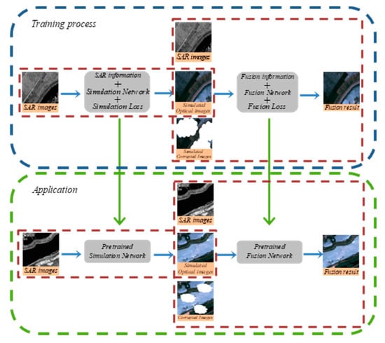
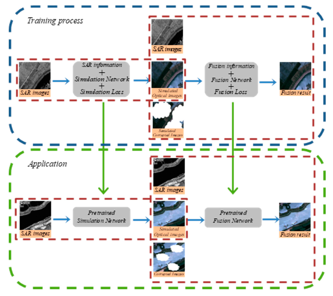
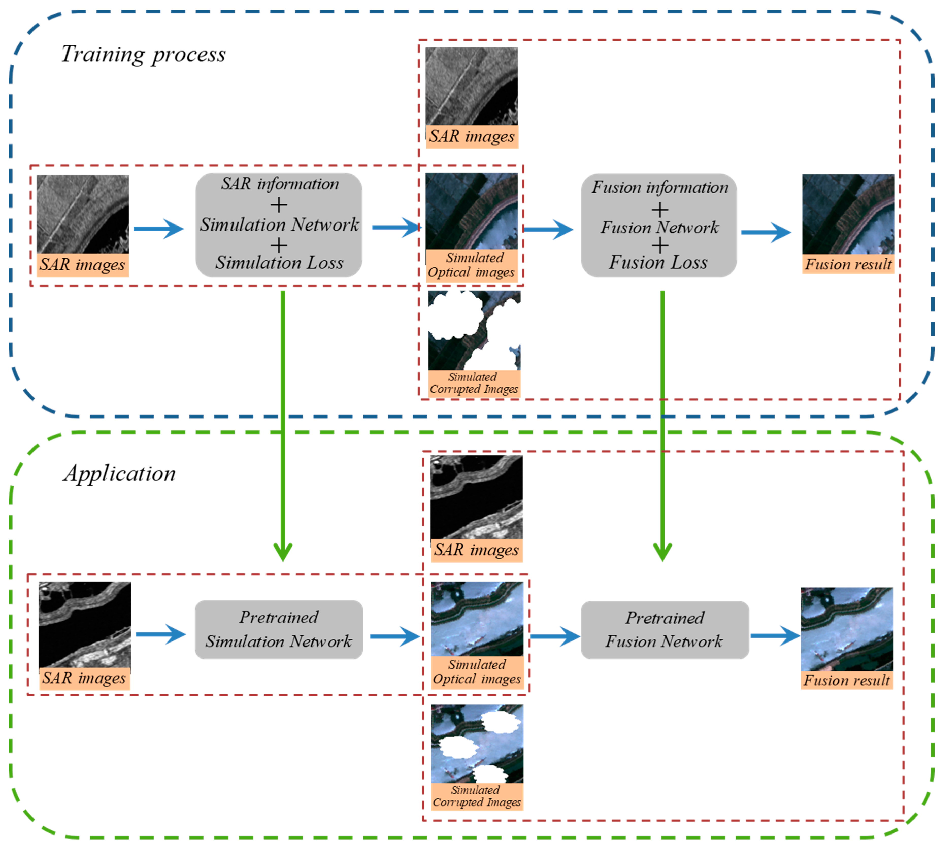
The proposed framework covers two main stages and some special data processing is conducted between the two stages. Before the cloud removal processing, coregistration and resolution unification of SAR/optical data are completed. In the first stage, the SAR data is translated into a simulated optical image with coarse texture and low spectrum accuracy by a special convolutional neural network (CNN) model. Before the second stage, the simulated optical image randomly altered its contrast and luminance. The reason for this operation is to make the model of the fusion stage robust because CNN in the first stage may generate an output with wrong spectral information in some cases. In the second stage, the SAR data, the simulated optical image and the real optical image corrupted by clouds are fused jointly to reconstruct the missing parts and we finally get a cloud-free output with proper spectral accuracy and high-frequency texture. Before the application, the whole network is pretrained with cloud-free parts of the corrupted optical image or the cloud-free optical image from another time. The overall flowchart of the proposed framework is displayed in Figure 1.
2.2. Simulation Process
Inspired by the great success in style transfer work achieved by deep learning, we introduced a classical deep learning model U-net [35], which shows its superiority in semantic segmentation tasks as the simulation network to translate a SAR image to an optical image in an object-to-object manner. In this process, we wish to obtain simulated optical images with similar spectral information to the ground truth and accurate object-to-object mapping. The structure of the network and the loss function are provided detailed in the following.
2.2.1. Network Structure
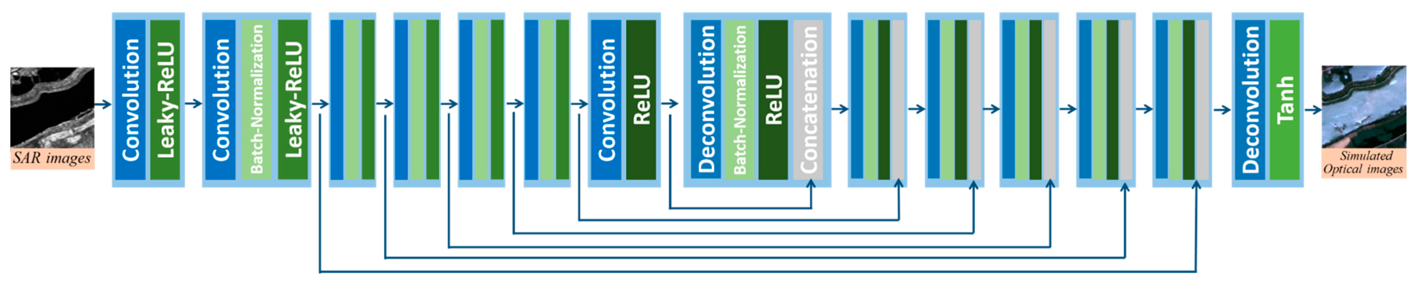
The structure of the simulation network together with its working process is presented in Figure 2, which is a 14-layer deep convolution neural network named U-net. The SAR imagery is input to this network and simulated optical imagery would be obtained as an output. The first seven layers are down-sampling layers, which may include a convolution layer acting down-sampling operation, a batch normalization layer and an activation layer. The last seven layers are up-sampling layers, which may include a convolution layer acting up-sampling operation, a batch-normalization layer and an activation layer. In addition, a skip connection operation is conducted in order between the first down-sampling layer and the up-sampling layer. This structure could reduce the information loss of input data during the operation within the network and make use of the high-level information and the low-level information at the same time. Compared with other deep learning models, U-net has a deeper structure to extract high-level features while training faster. In general, this structure perfectly meets our demand for translation from SAR images to optical images.
2.2.2. Loss Function
A traditional but effective loss function L1 is provided to constrain the output simulated optical image. This loss function would make the output clearer and have acute edges. So, the optimization of the network can be defined as:
stands for the Simulation Network and GT means the ground truth optical image.
2.3. Fusion Process
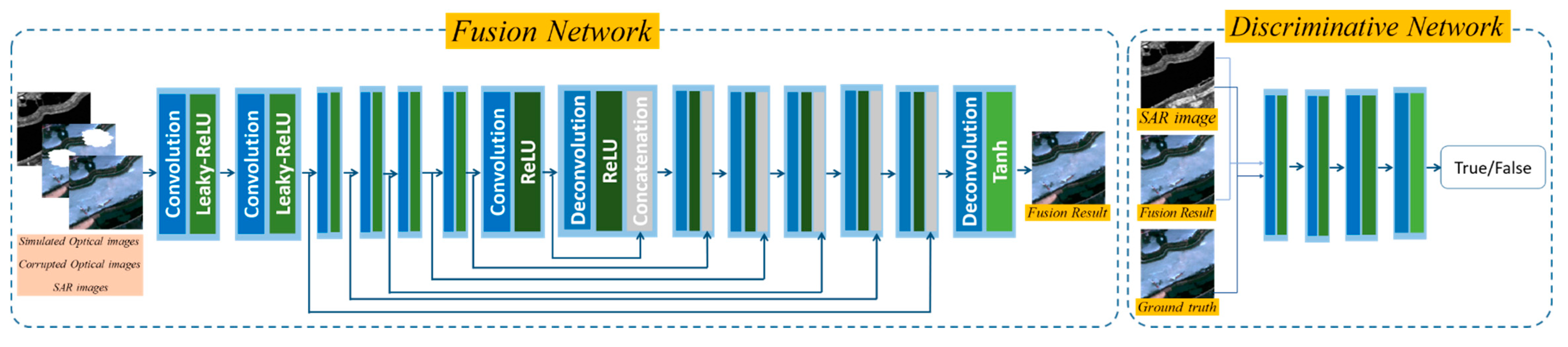
Although the simulated optical image has relatively correct spectral information and can roughly reflect the situation of the ground truth, two main drawbacks still constrain its application. On the one hand, a tiny deviation of spectral information still exists between the simulated optical image and ground truth, which makes the simulated optical image unable to perfectly substitute the ground truth. On the other hand, some high-frequency details such as texture cannot be generated in the simulation process due to the lack of information in SAR imagery and the limitation of the model. Aiming at solving these two drawbacks, we introduce the generative adversarial network (GAN) as the fusion network to fuse the simulated optical image, SAR, and the corrupted optical image to obtain an output with proper spectral information and fine texture in the fusion process. The workflow, structure and loss function of GAN are demonstrated below in detail. As is displayed in Figure 3, the generative adversarial network contains two working parts: a generative network and a discriminative network.
2.3.1. Generative Adversarial Network for Fusion
The generative network is expected to fuse the simulated optical image, SAR and the corrupted optical image to obtain a fusion result that cannot be distinguished from the ground truth by the discriminative network, but the discriminative network tries to distinguish the fusion result from the ground truth to urge the generative network get better results. The two networks are alternately optimized so that adversarial learning is formed between them. Finally, the generative network can be employed to accomplish the fusion work when reaching the Nash equilibrium [36].
The structure of the generative network and discriminative network are also shown in Figure 3. The generative network adapts a 14-layer U-net structure just like the first stage. Specially, we modify the model by removing all of the Batch-Normalization layers to avoid its effect on global distribution. The concatenation of the simulated optical image, SAR and the corrupted optical image is taken as the input of the generative network, in which SAR data restricts the global structure, the corrupted optical image is a reference data of spectral and texture information and the simulated optical image provides the reference in missing parts. Fusion results with proper spectral information and high-frequency texture are expected as the output.
The discriminative network is a simple convolution neural network with four layers. The first two layers respectively contain a convolution layer performing downsampling operation a Batch-Normalization layer and an activation layer, while the last two layers include a convolution layer and an activation layer. In consideration of controlling the global structure of the output from the generative network, the SAR image is taken into the discriminative network as auxiliary data jointly with ground truth or fusion results and these two should be respectively judged as ‘True’ and ‘False’ by the discriminative network.
Actually, the fusion network is mainly based on the pix2pix model. However, during the experiments we found that the normalization layers in the pix2pix model would be counter-productive in processing remote sensing data. So, the normalization layers are removed and the final fusion network is thus obtained.
2.3.2. Loss Function
According to the generative network and the discriminative network defined above, a training strategy is developed and the loss functions are designed for this process. The discriminative network is optimized firstly. Considering that the concatenation of SAR and the fusion result should be judged as ‘False’ and the concatenation of SAR and the ground truth should be judged as ‘True’ by the discriminative network, a least square loss function was constructed to optimize the discriminative network:
represents the discriminative network and means the fusion network. and are respectively the corrupted optical image and the simulated optical image. is optimized once in each iteration of the training process. Then the optimized is fixed to optimize the fusion network by forcing to obtain a result that can be judged as ‘True’ by the fixed :
and are alternatively optimized according to the training strategy described above to form adversarial learning.
Although fusion results with tiny texture and great visual effect can be obtained, the global distribution still needs restriction to get a better result with a traditional loss function like L1:
In addition, studies have shown that the perceptual loss function [37] can lead to results with better visual perception. We extract feature maps of the fusion result and the ground truth from the 8th layer of VGG16 to construct a perceptual loss function:
Here stands for the fusion result.
The loss functions defined above are mainly aimed at reconstructing the corrupted image from a global view. Furthermore, a loss function should be designed to especially focus on the restoration of the missing parts. Thus we take advantage of the cloud mask M to construct a local loss function for local reconstruction:
The total loss function of the fusion network, which contains both global and local loss functions is finally obtained:
in which ,, and are respectively the weight of the ,, and .
With the fixed discriminative network , the fusion network is optimized by gradient descent algorithm according to the Equation (7). Then the gets fixed to optimize the discriminative network according to Equation (2) again. The two networks are alternatively optimized with the training strategy demonstrated above until the Nash Equilibrium. At last, the optimized could be employed to conduct the fusion task.
2.4. Data Disturbance
We had an assumption that the simulated optical image obtained from the first stage has similar spectral information with the ground truth. However, when the acquisition time between testing data and training data is inconsistent, the situation may exist that the output of simulation network presents very different spectral information with ground truth. Thus a horrible fusion result will be generated if the simulation optical image with wrong spectral information is processed as a fusion material in the second stage. In this case, a necessity arouses that the fusion model should be more robust when dealing with the simulated optical image with a certain bias in its spectrum information from the ground truth. So, we randomly alter the contrast and luminance for each band of the simulated optical image before the fusion process to make the model of fusion process more robust and further able to be applied in other periods. The random transformation function is calculated as follows:
and respectively mean the random contrast alternation operation and random luminance alternation operation. then takes the place of as the input to the .
3. Experimental Results and Analysis
3.1. Settings
In order to verify the feasibility of our framework on the cloud removal task, simulated and real-world experiments were conducted with different datasets. Settings of the experiments including datasets, training settings, evaluation methods and compared algorithms are presented in detail as follows.
3.1.1. Datasets
We collected two datasets, namely Dataset A and Dataset B, to conduct the simulated experiments and one dataset, namely Dataset C to conduct the real experiment.
Dataset A is made by data from GF-2 and GF-3 with a size of 3742 px × 2947 px in Nanchang, Jiangxi Province, China. The land cover types are mainly farmlands and rivers, which is somehow simple and with less texture. The GF-2 optical image was acquired on August 12 2016 with a resolution of 3.2 m. The GF-3 SAR image was acquired on August 16 2016 with a resolution of 1 m. The two images are roughly coregistered with a deviation of fewer than 5 pixels. This dataset also proved that the neural network model could also work when tiny deviations exist between the SAR and optical images.
The SAR and optical data in Dataset B were provided in the 2001 IEEE GRSS data fusion contest with a size of 2813 px × 2289 px. The land cover types are mainly houses, roads and farmlands, which are relatively complex and with dense texture. The SAR and optical data are finely coregistered and shared the same resolution of 1 m. Before the experiment, the SAR image is denoised by the SAR-BM3D [38] algorithm.
Dataset C employs SAR data from Sentinel-1 and optical data from Sentinel-2, which are acquired from Kempten city, Germany. The Sentinel-1 SAR data was acquired on Mar. 5 2017 whose polarization mode is hh and resolution is 5 m. The Sentinel-2 optical image was acquired on Jul. 16 2017, of which we make use of three bands including R, G and B with a resolution of 10 m. We have made sure that no large changes occurred between this time gap. The SAR and optical data whose size are both 1024 px × 1024 px are roughly coregistered with a deviation of fewer than 5 pixels.
Images in Dataset A and B are cropped into 128 px × 128 px. Corrupted areas were imposed on the optical images to simulate the cloud in around 35% of the area. Ninety percent of the images of the dataset are used as the training dataset and the rest 10% images are used to test the model. For Dataset C, the model is pretrained with data from another time, then the whole SAR image and optical image are input to the model to get a cloud removal result.
3.1.2. Cloud Simulation and Detection
In the simulation experiments, we produce cloud masks manually in the Photoshop software. First, we randomly draw around 100 cloud figures, which take up about 35% of the whole area. Then these figures are randomly rotated, up-sampled/down-sampled and crop to obtain more figures. Finally, the figures whose corrupted area is larger than 40% or smaller than 30% are filtered out because the statistics show that the proportion of land area covered by cloud is around this range. The rest figures are used as cloud masks in the simulation experiment.
Between the simulation and fusion process, cloud detection work of the real optical image is indispensable in order to construct a certain loss function in the second stage and analysis the reconstruction results in the end. Many efficient models have so far been proposed to detect the clouds and its accompanying shadows, such as Fmask [39] and MSCFF [40]. We thus adapt MSCFF, which is based on deep learning, to detect the clouds and get a binary map MC of the clouds.
3.1.3. Training Settings
We adopt the Adam optimization algorithm to optimize the network and the hyperparameters were set as and . The learning rate is set as 0.0002 in the first 75 epochs and gradually decayed to 0 in the last 75 epochs. In addition, the weights of loss function defined in Section 2 were respectively , , and .
3.1.4. Evaluation Indicators
Four quantitative indexes are selected to evaluate the results of simulated experiments. The first two indexes are root mean squared error (RMSE) and spectral angle mapping (SAM). The smaller the values are, the better the results will be. The last two indexes are mean structure similarity index measurement [36] (mSSIM) and correlation coefficient (CC) The larger the values are, the better results will be obtained. Moreover, visual evaluation is applied to observe the reconstruction details.
3.1.5. Compared Algorithms
Among the cloud removal algorithms mentioned in Section 1, two deep-learning-based algorithms that utilized single-temporal SAR and optical data are selected to compare with our method: pix2pix model [31] and SAR-opt-GAN model [32]. The pix2pix model adopts a conditional GAN model to directly translate the SAR images to optical images with paired SAR/optical data and GAN training strategy demonstrated above. The land cover types of result images can be greatly classified. SAR-opt-GAN model also employs a conditional GAN model and training strategy as the pix2pix model. However, the input of the model is the concatenation of SAR and corrupted optical image and the result is expected to be a cloud-free optical image. In fact, this model does have an advantage in thin cloud removal work. The above-mentioned compared algorithms and the proposed algorithm are trained on the same datasets.
3.2. Simulated Experiment
3.2.1. Results of Dataset A
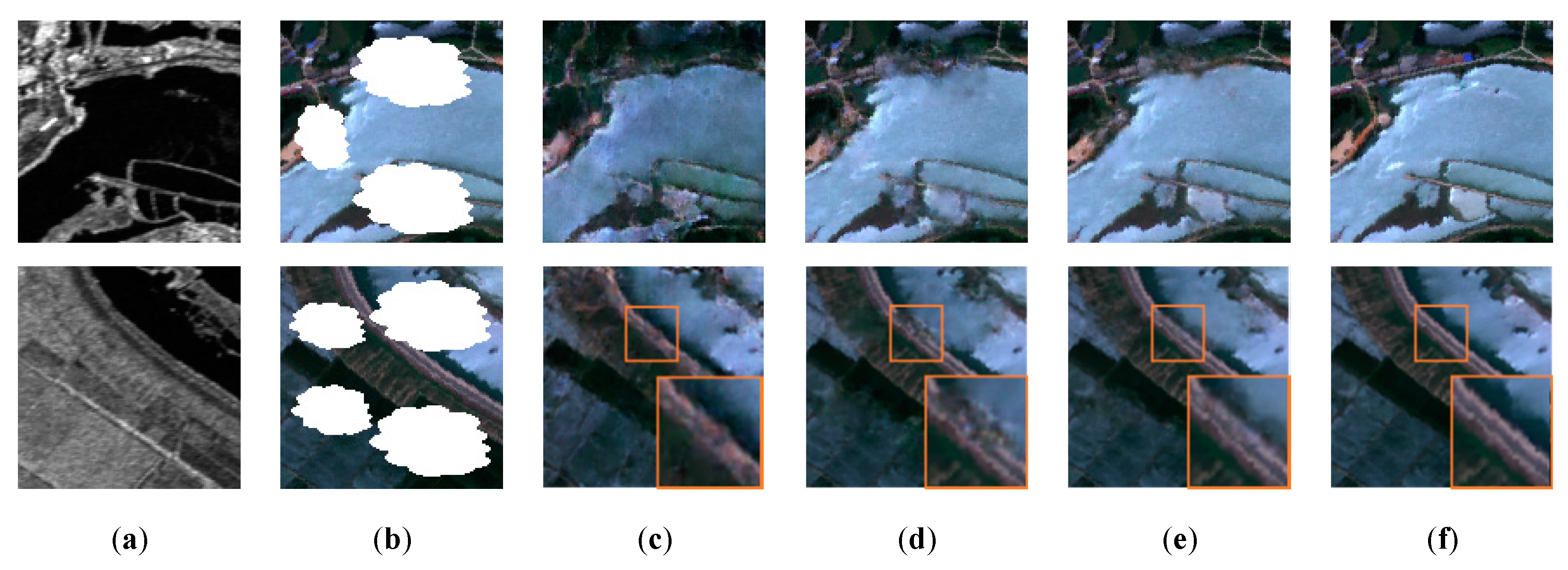
The experiment results of Dataset A are displayed in Figure 4. The SAR images are shown in Figure 4a and the simulated corrupted images are exhibited in Figure 4b. Results of the pix2pix model, SAP-opt-GAN model and the proposed model are respectively displayed in Figure 4c–e. Figure 4f displays the ground truth. Furthermore, Table 1 list the quantitative evaluation results including RMSE, mSSIM, CC and SAM.
As is shown in the first row in Figure 4, the result generated by the pix2pix model has a deviation on spectral information from the ground truth. In contrast, SAR-opt-GAN model and the proposed model outperforms in reconstructing the spectral information of ground truth images. Quantitative evaluation results listed in Table 1 confirm that the SAR-opt-GAN model and the proposed model could generate great results to some degree, but the proposed model performed better than the above two models. In addition, the proposed model outperforms the other two models in terms of tiny ground objects reconstruction. We could observe that in the second row of Figure 4, SAR-opt-GAN model could not restore the road, which is magnified. The pix2pix model just generates a result in which almost no road is reconstructed. However, the proposed model could precisely restore this tiny object. In general, the proposed model shows its superiority in terms of spectral restoration and ground object construction compared with the pix2pix model and SAR-opt-GAN model. The experiment results of Dataset B are shown in Figure 5.
3.2.2. Results of Dataset B
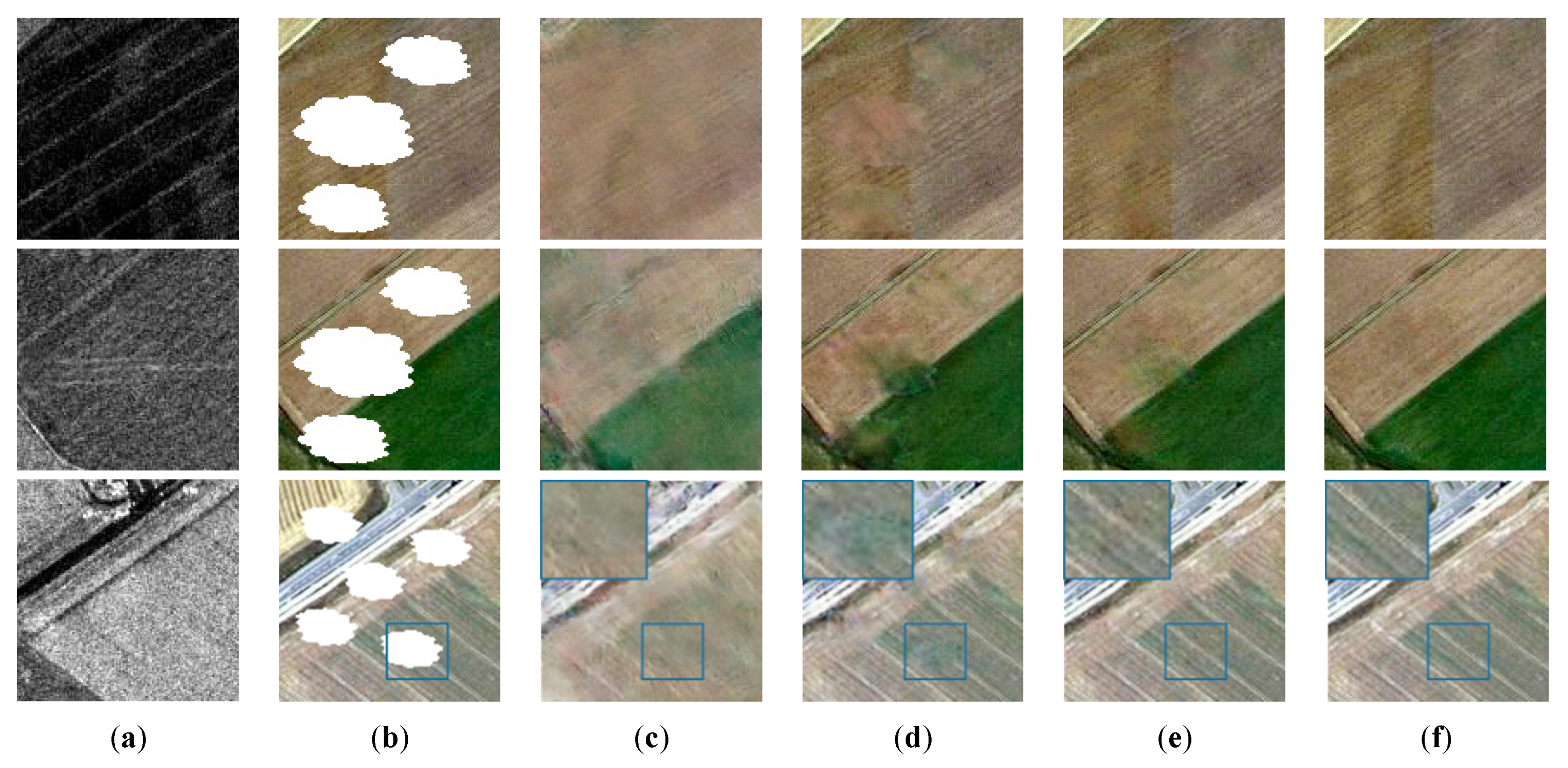
Figure 5a,b stands for the SAR images and the simulated. Results of the pix2pix model, SAR-opt-GAN model and the proposed model are displayed in Figure 5c–e. Ground truth images are exhibited in Figure 5f. Moreover, quantitative evaluation results including RMSE, mSSIM, CC and SAM are enumerated in Table 2
In Dataset B, spectral deviation still exists in the results of the pix2pix model just as the first row of Figure 5 shows, but SAR-opt-GAN and the proposed model are freed from this issue again because they take the remainder of corrupt optical images as reference data. Nonetheless, as is shown in the second row of Figure 5, SAR-opt-GAN generates results with apparent artifacts nearby the corrupted areas, showing the limitation of SAR-opt-GAN model. However, the results of pix2pix model and the proposed model have barely artifacts relatively. In addition, a local area is magnified to observe the texture reconstruction of the three models in the third row of Figure 5. It is clear that pix2pix model and SAR-opt-GAN model have a poor ability to restore the texture information of the ground truth but the proposed model shows its advantage in texture generation, which means that the proposed model could handle more complex images. Quantitative evaluation results also prove the superiority of the proposed model in Table 2. In general, the proposed model still performs well in terms of spectral fidelity, artifacts removal and texture generation. Figure 6d–f stands for the global reconstruction results of the pix2pix model, SAR-opt-GAN model and the proposed model.
3.3. Real Experiment
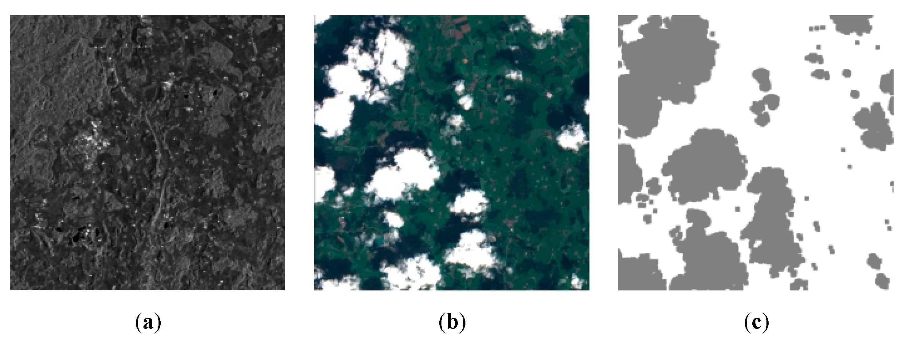
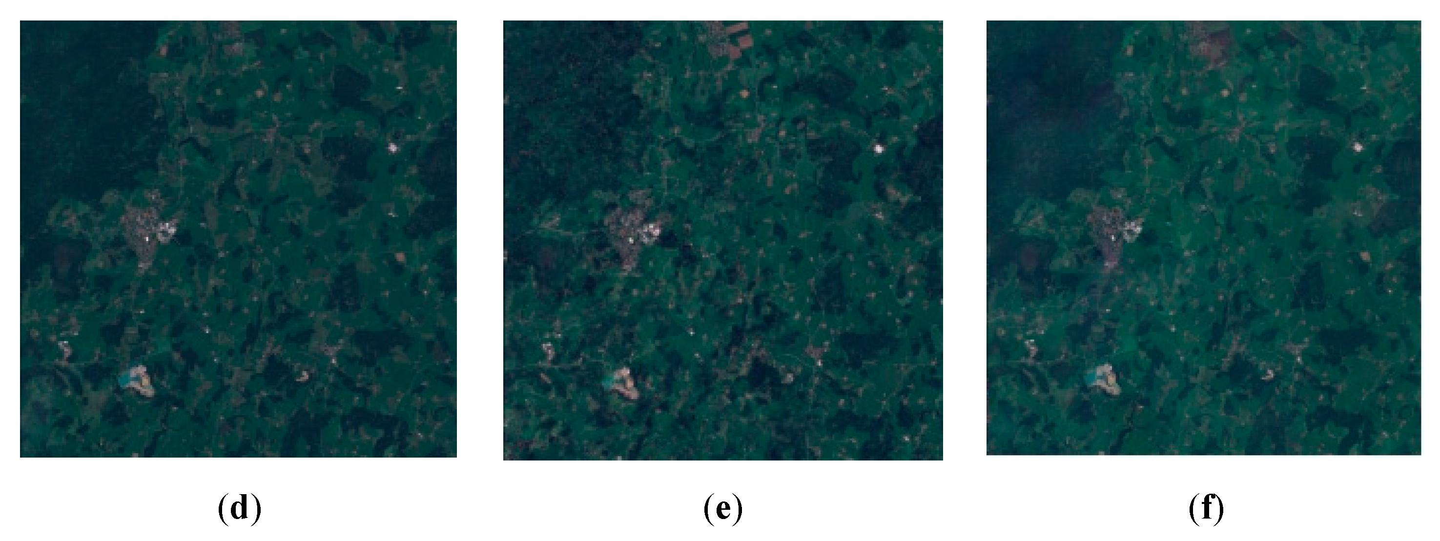
In order to validate that the proposed method is applicable to the real situation, we conduct a real-world experiment with Dataset C. The corrupted area of optical data accounts for 38.38% of the total area according to the calculation of MSCFF [40]. The real experiment results are displayed in Figure 6. Figure 6a–c is the SAR image, the corrupted optical image and the cloud mask obtained by MSCFF.
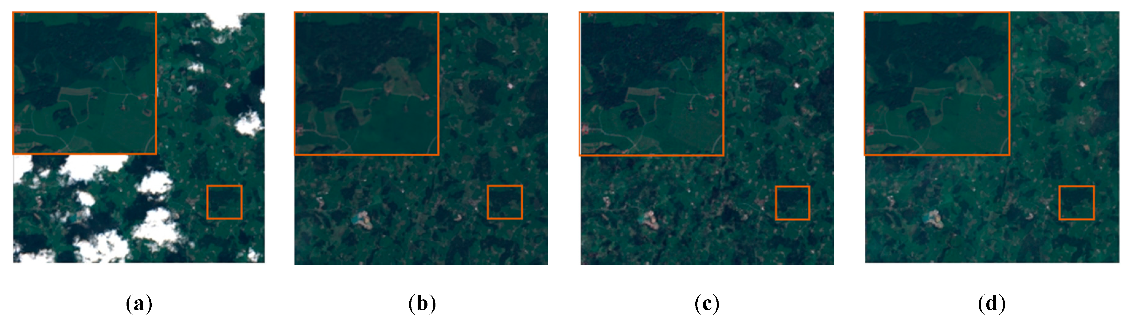
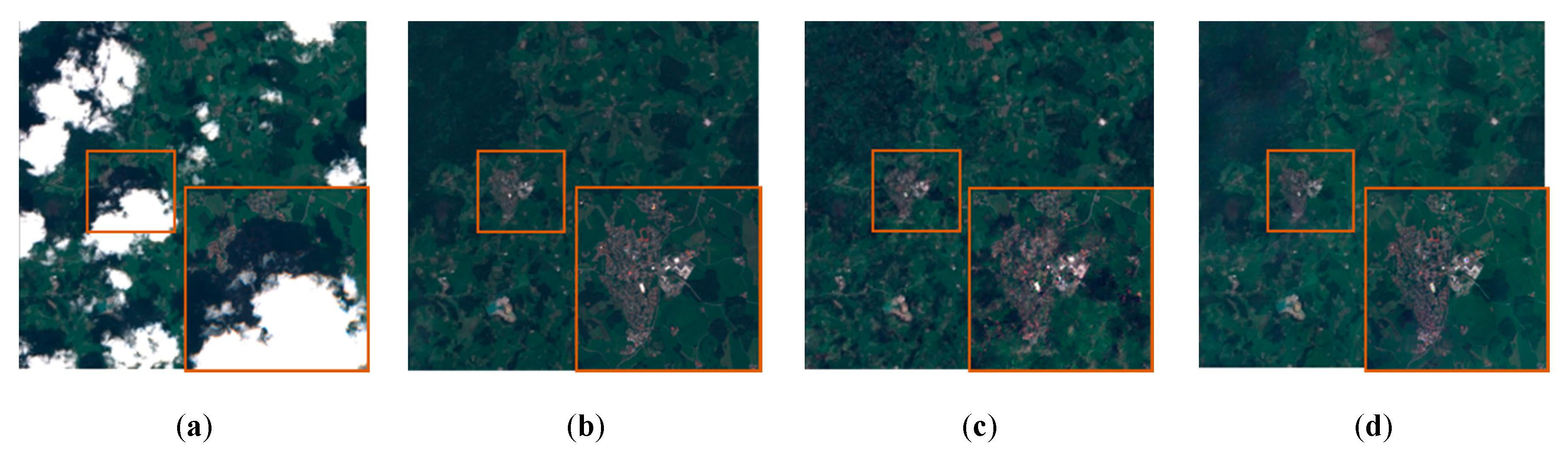
Then some areas were selected to evaluate the reconstruction from a local view. Figure 7, Figure 8 and Figure 9 present the reconstruction results of these selected areas. Figure 7, Figure 8 and Figure 9a display the selected corrupted optical images. b–d from Figure 7, Figure 8 and Figure 9 display the reconstruction results of the pix2pix model, SAR-opt-GAN model and the proposed model respectively.
Generally, we could observe that all three models achieve results with great visual effects from a global view in Figure 6. However, certain performance differences are observed between the three models in some local areas. The area shown in Figure 7 is selected from a cloud-free area of the optical image, which could be viewed as ground truth. The reconstruction result of the pix2pix model has an obviously darker spectral information compared with the ground truth, while the results obtained by SAR-opt-GAN model and the proposed model largely retain the proper spectral information of the ground truth. Figure 8 displays a junction between the corrupted and cloud-free areas. The result of SAR-opt-GAN has a vivid boundary around the junction part, but the proposed model and the pix2pix model obtain results with no boundary trace nearby the corresponding part. Figure 9 presents an urban area with relatively complex texture information. The pix2pix model and the proposed model could reconstruct the corrupted parts with clear details but SAR-opt-GAN just generates a result with fuzzy ground objects on it.
As a whole, our method outperforms the other two methods in terms of several visual evaluations including spectral fidelity, inpainting effect and reconstruction of objects.
3.4. Discussion
3.4.1. Ablation Study of the Model
As is demonstrated in Section 2, the proposed model includes three main operations: simulation process, data disturbance process and fusion process. In this part, three ablation models would be compared with the proposed model to display the importance of these operations. The three ablation models are respectively the model without simulation process, the model without fusion process and the model without data disturbance process. Dataset B is applied in this study and the results of these ablation models and the proposed model are listed in Table 3.
According to Table 3 it goes without saying that the results of model without fusion process and model without simulation process degrade a lot compared with the proposed model. It is also important to mention that certain data disturbance on the simulated optical image would really improve the final fusion results. It confirms our idea that data disturbance might strengthen the robustness of the fusion network. We explore the impact of different terms of our reconstruction loss functions including L1 loss, GAN loss, perceptual loss and local loss. Each of the four loss terms in the original model is ablated alternately to get four ablation models. Then the results of the ablation models and original model are compared to evaluate the importance of each loss term. Dataset B is again applied in this section and the evaluation results of different ablation models are listed in Table 4.
3.4.2. Ablation Study of the Loss Functions
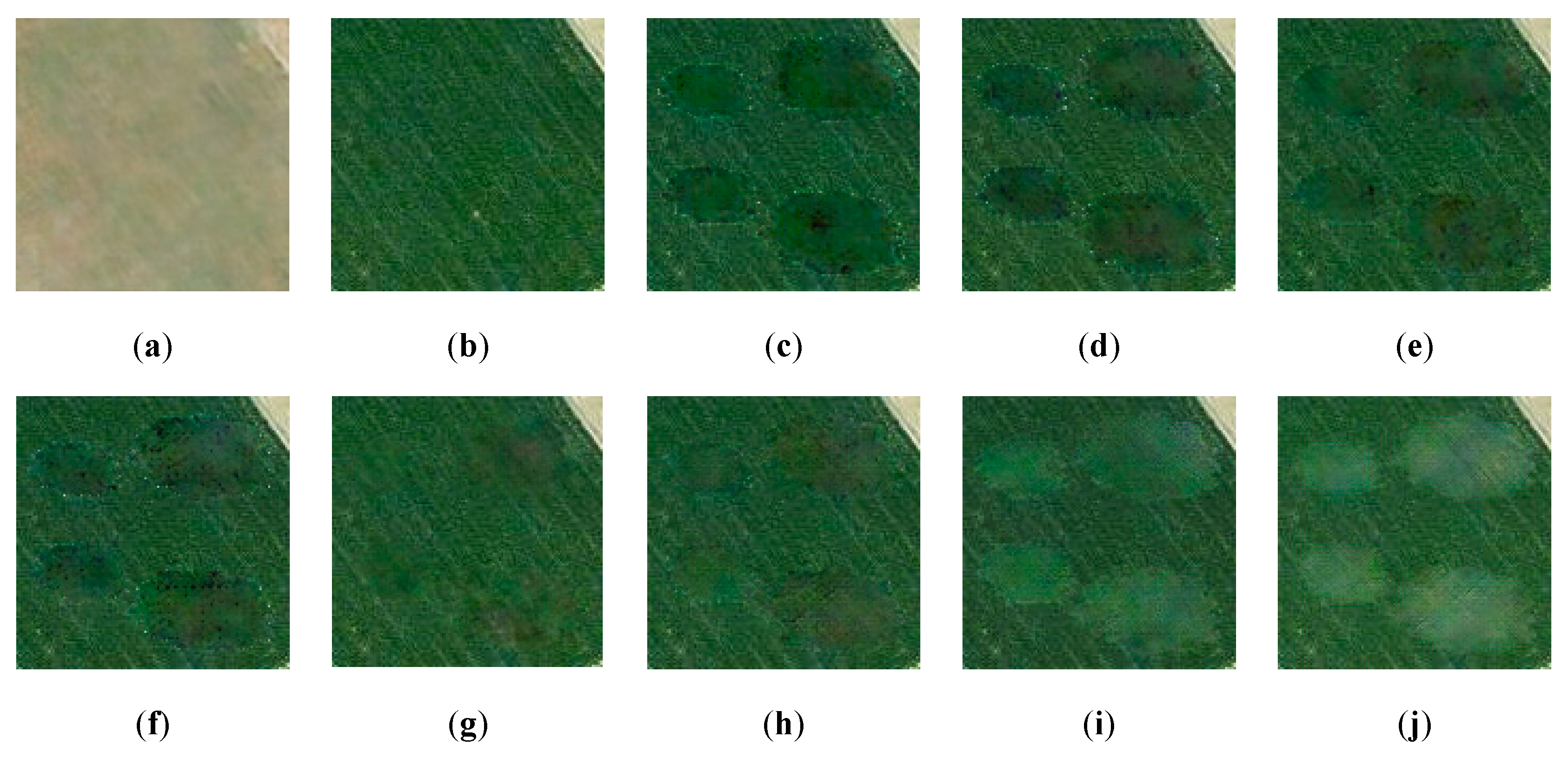
In Figure 10, a case that simulation network fails to work and generate an output with different spectrum, which is shown in Figure 10c. The model without perceptual loss would get obvious ‘patches’ in no harmony with surroundings in the corresponding missing parts. However, the original model overcame this failure, which is shown in Figure 10d because perceptual loss is conducted by the feature map from the vgg16 network, which is able to extract the boundary if the ‘filling patches’ have different color with surroundings in the fusion result.
The model without L1 loss could also generate a similar result compared with the original model but fails to control the global distribution of the output as well as the original model. Model without local loss achieves similar results to the original model, but degradation actually appears according to the quantitative evaluation in Table 3. Results generated by model without GAN loss would also degrade a little in the quantitative evaluation compared to the original model.
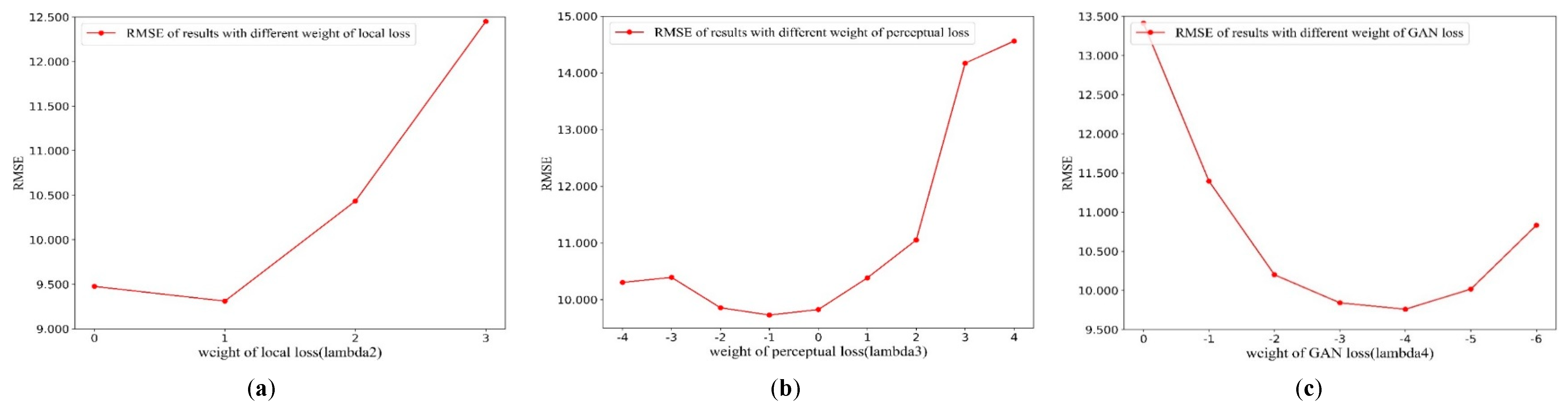
What could also be observed from Table 3 is that the perceptual loss term seems to have a retroaction toward the result, but it enriches the texture information, which is reflected in mSSIM index and does increase the robustness of the model to some degree. As varies from 101 to 104, which is plotted in Figure 11a, the model achieves the lowest RMSE when equals 102. Then is the weight of perceptual loss term. It can be observed from Figure 11b that the perceptual loss term seems counterproductive to the result.
3.5. Parameter Sensitive Analysis
In this part, we pay attention to analyzing the parameters given in the loss function: ,, and to fine-tune the model to the best. Since there are four parameters and coupling might exist between different loss functions, the strategy is given that the loss terms are added one by one in the order of magnitude. We first fix the weight of L1 as 10 and add the local loss to ensure its weight . The weight of perceptual loss term is afterward affirmed and the weight of GAN loss term is final. To quantitatively evaluate the results, RMSE was applied to compare models with different weight.
However, as is displayed in Figure 12, appropriate weight of perceptual loss would alleviate the existence of filling patches with a different color mentioned in the ablation study. So, we set the as 0.8. Finally, the results would be best when the weight of GAN loss is set to 10−4 as varies from 10−6 to 104, which is plotted in Figure 12c.
4. Conclusions
In this work, a framework called Simulation-Fusion GAN was proposed for cloud removal tasks of optical remote sensing data, taking advantage of GAN model as the basic structure and SAR data as the reference data. Differing from the methods applying direct translation from a SAR data to an optical data or direct fusion of SAR and optical data, we carefully settled the simulation and fusion process and optimized the model with a special-designed loss function. In this process, the relationship between SAR and optical images was learning sufficiently and the residual spectral information of corrupted optical images was utilized at the same time. The outperformance of experimental results on GF-2/3, airborne SAR/optical data and sentinel-1/2 all confirmed the feasibility and validity of our model.
Although the proposed method acquired satisfying results and outperformed other similar methods, there are still some limitations to overcome. One is that the different models should be pretrained every time in different certain place. In future work, we will take advantage of the multitemporal data and take change detection into consideration to make the model be more robust and have generalization ability. In addition, the land cover classification on the reconstruction results will be considered afterward.
Author Contributions
Conceptualization, J.G., Q.Y. and J.L.; Formal analysis, J.G.; Funding acquisition, J.L.; Investigation, J.G.; Methodology, J.G., Q.Y. and J.L.; Project administration, Q.Y. and J.L.; Resources, Q.Y. and J.L.; Supervision, Q.Y., J.L., H.Z. and X.S.; Validation, J.G.; Writing—original draft, J.G. and J.L.; Writing—review & editing, Q.Y., H.Z. and X.S. All authors have read and agreed to the published version of the manuscript.
Funding
This research was funded by National Natural Science Foundation of China, grant number 61971319, 41701400, 41922008 and 64671334; China Postdoctoral Science Foundation, grant number 2018T110803.
Conflicts of Interest
The authors declare no conflicts of interest.
References
- Ju, J.; Roy, D.P. The availability of cloud-free landsat etm plus data over the conterminous United States and globally. Remote Sens. Environ. 2008, 112, 1196–1211. [Google Scholar] [CrossRef]
- Shen, H.; Li, X.; Cheng, Q.; Zeng, C.; Yang, G.; Li, H.; Zhang, L. Missing information reconstruction of remote sensing data: A technical review. IEEE Geosci. Remote Sens. Mag. 2015, 3, 61–85. [Google Scholar] [CrossRef]
- Wang, L.; Qu, J.J.; Xiong, X.; Hao, X.; Xie, Y.; Che, N. A new method for retrieving band 6 of aqua modis. IEEE Geosci. Remote Sens. Lett. 2006, 3, 267–270. [Google Scholar] [CrossRef]
- Rakwatin, P.; Takeuchi, W.; Yasuoka, Y. Restoration of aqua modis band 6 using histogram matching and local least squares fitting. IEEE Trans. Geosci. Remote Sens. 2009, 47, 613–627. [Google Scholar] [CrossRef]
- Shen, H.; Zeng, C.; Zhang, L. Recovering reflectance of aqua modis band 6 based on within-class local fitting. IEEE J. Sel. Top. Appl. Earth Obs. Remote Sens. 2011, 4, 185–192. [Google Scholar] [CrossRef]
- Gladkova, I.; Grossberg, M.D.; Shahriar, F.; Bonev, G.; Romanov, P. Quantitative restoration for modis band 6 on aqua. IEEE Trans. Geosci. Remote Sens. 2012, 50, 2409–2416. [Google Scholar] [CrossRef]
- Shen, H.; Li, X.; Zhang, L.; Tao, D.; Zeng, C. Compressed sensing-based inpainting of aqua moderate resolution imaging spectroradiometer band 6 using adaptive spectrum-weighted sparse bayesian dictionary learning. IEEE Trans. Geosci. Remote Sens. 2014, 52, 894–906. [Google Scholar] [CrossRef]
- Zhang, C.; Li, W.; Travis, D. Gaps-fill of slc-off landsat etm plus satellite image using a geostatistical approach. Int. J. Remote Sens. 2007, 28, 5103–5122. [Google Scholar] [CrossRef]
- Yu, C.; Chen, L.; Su, L.; Fan, M.; Li, S. Kriging interpolation method and its application in retrieval of modis aerosol optical depth. In Proceedings of the 2011 19th International Conference on Geoinformatics, Shanghai, China, 24–26 June 2011; pp. 1–6. [Google Scholar]
- Maalouf, A.; Carre, P.; Augereau, B.; Fernandez-Maloigne, C. A bandelet-based inpainting technique for clouds removal from remotely sensed images. IEEE Trans. Geosci. Remote Sens. 2009, 47, 2363–2371. [Google Scholar] [CrossRef]
- Mendez-Rial, R.; Calvino-Cancela, M.; Martin-Herrero, J. Anisotropic inpainting of the hypercube. IEEE Geosci. Remote Sens. Lett. 2012, 9, 214–218. [Google Scholar] [CrossRef]
- Shen, H.; Zhang, L. A map-based algorithm for destriping and inpainting of remotely sensed images. IEEE Trans. Geosci. Remote Sens. 2009, 47, 1492–1502. [Google Scholar] [CrossRef]
- Cheng, Q.; Shen, H.; Zhang, L.; Li, P. Inpainting for remotely sensed images with a multichannel nonlocal total variation model. IEEE Trans. Geosci. Remote Sens. 2014, 52, 175–187. [Google Scholar] [CrossRef]
- Criminisi, A.; Perez, P.; Toyama, K. Region filling and object removal by exemplar-based image inpainting. IEEE Trans. Image Process. 2004, 13, 1200–1212. [Google Scholar] [CrossRef] [PubMed]
- Lin, C.; Tsai, P.; Lai, K.; Chen, J. Cloud removal from multitemporal satellite images using information cloning. IEEE Trans. Geosci. Remote Sens. 2013, 51, 232–241. [Google Scholar] [CrossRef]
- Zeng, C.; Shen, H.F.; Zhang, L.P. Recovering missing pixels for landsat etm plus slc-off imagery using multi-temporal regression analysis and a regularization method. Remote Sens. Environ. 2013, 131, 182–194. [Google Scholar] [CrossRef]
- Shen, H.; Wu, J.; Cheng, Q.; Aihemaiti, M.; Zhang, C.; Li, Z. A spatiotemporal fusion based cloud removal method for remote sensing images with land cover changes. IEEE J. Sel. Top. Appl. Earth Obs. Remote Sens. 2019, 12, 862–874. [Google Scholar] [CrossRef]
- Li, Z.; Shen, H.; Cheng, Q.; Li, W.; Zhang, L. Thick cloud removal in high-resolution satellite images using stepwise radiometric adjustment and residual correction. Remote Sens. 2019, 11, 1925. [Google Scholar] [CrossRef] [Green Version]
- Chen, J.; Jonsson, P.; Tamura, M.; Gu, Z.H.; Matsushita, B.; Eklundh, L. A simple method for reconstructing a high-quality ndvi time-series data set based on the savitzky-golay filter. Remote Sens. Environ. 2004, 91, 332–344. [Google Scholar] [CrossRef]
- Lorenzi, L.; Melgani, F.; Mercier, G. Missing-area reconstruction in multispectral images under a compressive sensing perspective. IEEE Trans. Geosci. Remote Sens. 2013, 51, 3998–4008. [Google Scholar] [CrossRef]
- Li, X.; Shen, H.; Zhang, L.; Zhang, H.; Yuan, Q.; Yang, G. Recovering quantitative remote sensing products contaminated by thick clouds and shadows using multitemporal dictionary learning. IEEE Trans. Geosci. Remote Sens. 2014, 52, 7086–7098. [Google Scholar]
- Zhang, Q.; Yuan, Q.; Zeng, C.; Li, X.; Wei, Y. Missing data reconstruction in remote sensing image with a unified spatial–temporal–spectral deep convolutional neural network. IEEE Trans. Geosci. Remote Sens. 2018, 56, 4274–4288. [Google Scholar] [CrossRef] [Green Version]
- Li, W.B.; Li, Y.; Chen, D.; Chan, J.C.W. Thin cloud removal with residual symmetrical concatenation network. ISPRS J. Photogramm. Remote Sens. 2019, 153, 137–150. [Google Scholar] [CrossRef]
- Dong, J.; Yin, R.; Sun, X.; Li, Q.; Yang, Y.; Qin, X. Inpainting of remote sensing sst images with deep convolutional generative adversarial network. IEEE Geosci. Remote Sens. Lett. 2019, 16, 173–177. [Google Scholar] [CrossRef]
- Singh, P.; Komodakis, N. IEEE Cloud-gan: Cloud removal for sentinel-2 imagery using a cyclic consistent generative adversarial networks. In Proceedings of the IGARSS 2018–2018 IEEE International Geoscience and Remote Sensing Symposium, Valencia, Spain, 22–27 July 2018; pp. 1772–1775. [Google Scholar]
- Zhu, J.-Y.; Park, T.; Isola, P.; Efros, A.A. Unpaired Image-To-Image Translation Using Cycle-Consistent Adversarial Networks. In Proceedings of the IEEE International Conference on Computer Vision (ICCV), Venice, Italy, 22–29 October 2017; pp. 2242–2251. [Google Scholar]
- Eckardt, R.; Berger, C.; Thiel, C.; Schmullius, C. Removal of optically thick clouds from multi-spectral satellite images using multi-frequency sar data. Remote Sens. 2013, 5, 2973–3006. [Google Scholar] [CrossRef] [Green Version]
- Huang, B.; Li, Y.; Han, X.; Cui, Y.; Li, W.; Li, R. Cloud removal from optical satellite imagery with sar imagery using sparse representation. IEEE Geosci. Remote Sens. Lett. 2015, 12, 1046–1050. [Google Scholar] [CrossRef]
- Liu, L.; Lei, B. Can sar images and optical images transfer with each other? In Proceedings of the IGARSS 2018–2018 IEEE International Geoscience and Remote Sensing Symposium, Valencia, Spain, 22–27 July 2018; pp. 7019–7022. [Google Scholar]
- Fuentes Reyes, M.; Auer, S.; Merkle, N.; Henry, C.; Schmitt, M. Sar-to-optical image translation based on conditional generative adversarial networks—Optimization, opportunities and limits. Remote Sens. 2019, 11, 2067. [Google Scholar] [CrossRef] [Green Version]
- Bermudez, J.D.; Happ, P.N.; Oliveira, D.A.B.; Feitosa, R.Q. Sar to optical image synthesis for cloud removal with generative adversarial networks. In ISPRS Mid-Term Symposium Innovative Sensing—From Sensors to Methods and Applications, Karlsruhe, Germany, 10–12 October, 2018; Jutzi, B., Weinmann, M., Hinz, S., Eds.; ISPRS: Leopoldshöhe, Germany, 2018; Volume 4, pp. 5–11. [Google Scholar]
- Grohnfeldt, C.; Schmitt, M.; Zhu, X. A conditional generative adversarial network to fuse sar and multispectral optical data for cloud removal from sentinel-2 images. In Proceedings of the IGARSS 2018–2018 IEEE International Geoscience and Remote Sensing Symposium, Valencia, Spain, 22–27 July 2018; pp. 1726–1729. [Google Scholar]
- Bermudez, J.D.; Happ, P.N.; Feitosa, R.Q.; Oliveira, D.A.B. Synthesis of multispectral optical images from sar/optical multitemporal data using conditional generative adversarial networks. IEEE Geosci. Remote Sens. Lett. 2019, 16, 1220–1224. [Google Scholar] [CrossRef]
- He, W.; Yokoya, N. Multi-temporal sentinel-1 and-2 data fusion for optical image simulation. ISPRS Int. J. Geo Inf. 2018, 7, 389. [Google Scholar] [CrossRef] [Green Version]
- Ronneberger, O.; Fischer, P.; Brox, T. U-net: Convolutional Networks for Biomedical Image Segmentation. In Medical Image Computing and Computer-Assisted Intervention, pt iii; Navab, N., Hornegger, J., Wells, W.M., Frangi, A.F., Eds.; Springer: New York, NY, USA, 2015; Volume 9351, pp. 234–241. [Google Scholar]
- Goodfellow, I.J.; Pouget-Abadie, J.; Mirza, M.; Xu, B.; Warde-Farley, D.; Ozair, S.; Courville, A.; Bengio, Y. Generative adversarial nets. In Advances in Neural Information Processing Systems 27, Montreal Canada, 8-13 December 2014; Ghahramani, Z., Welling, M., Cortes, C., Lawrence, N.D., Weinberger, K.Q., Eds.; Neural Information Processing Systems: San Diego, CA, USA, 2014; Volume 27. [Google Scholar]
- Johnson, J.; Alahi, A.; Li, F.-F. Perceptual losses for real-time style transfer and super-resolution. In Computer Vision—ECCV 2016, Amdterdam, Netherlands, 10–16 October 2016; Leibe, B., Matas, J., Sebe, N., Welling, M., Eds.; Springer: Cham, Switzerland, 2016; Volume 9906, pp. 694–711. [Google Scholar]
- Parrilli, S.; Poderico, M.; Angelino, C.V.; Verdoliva, L. A nonlocal sar image denoising algorithm based on llmmse wavelet shrinkage. IEEE Trans. Geosci. Remote Sens. 2012, 50, 606–616. [Google Scholar] [CrossRef]
- Qiu, S.; Zhu, Z.; He, B.B. Fmask 4.0: Improved cloud and cloud shadow detection in landsats 4–8 and sentinel-2 imagery. Remote Sens. Environ. 2019, 231, 111205. [Google Scholar] [CrossRef]
- Li, Z.W.; Shen, H.F.; Cheng, Q.; Liu, Y.H.; You, S.C.; He, Z.Y. Deep learning based cloud detection for medium and high resolution remote sensing images of different sensors. ISPRS J. Photogramm. Remote Sens. 2019, 150, 197–212. [Google Scholar] [CrossRef] [Green Version]
Figure 1.
Flowchart of the proposed model for cloud removal.

Figure 2.
Structure of the Simulation network.

Figure 3.
Structure of the fusion network.

Figure 4.
Results of each method in Dataset A. (a) original synthetic aperture radar (SAR) images; (b) simulated corrupted images; (c) results of the pix2pix model; (d) results of the SAR-opt- generative adversarial network (GAN) model; (e) results of the proposed model (f) ground truth.
Figure 4.
Results of each method in Dataset A. (a) original synthetic aperture radar (SAR) images; (b) simulated corrupted images; (c) results of the pix2pix model; (d) results of the SAR-opt- generative adversarial network (GAN) model; (e) results of the proposed model (f) ground truth.

Figure 5.
Results of each method in Dataset B. (a) original SAR images; (b) simulated corrupted images; (c) results of the pix2pix model; (d) results of the SAR-opt-GAN model; (e) results of the proposed model (f) ground truth.
Figure 5.
Results of each method in Dataset B. (a) original SAR images; (b) simulated corrupted images; (c) results of the pix2pix model; (d) results of the SAR-opt-GAN model; (e) results of the proposed model (f) ground truth.

Figure 6.
Overview of the results of the real experiment. (a) Original SAR image; (b) corrupted optical image; (c) cloud mask and (d) pix2pix model. (e) SAR-opt-GAN model; (f) the proposed model.
Figure 6.
Overview of the results of the real experiment. (a) Original SAR image; (b) corrupted optical image; (c) cloud mask and (d) pix2pix model. (e) SAR-opt-GAN model; (f) the proposed model.


Figure 7.
Results of Area 1 in the real experiment. (a) Ground truth of the optical image. (b) Pix2pix. (c) SAR-opt-GAN. (d) The proposed method.
Figure 7.
Results of Area 1 in the real experiment. (a) Ground truth of the optical image. (b) Pix2pix. (c) SAR-opt-GAN. (d) The proposed method.

Figure 8.
Results of Area 2 in the real experiment. (a) Ground truth of the optical image. (b) Pix2pix. (c) SAR-opt-GAN. (d) The proposed method.
Figure 8.
Results of Area 2 in the real experiment. (a) Ground truth of the optical image. (b) Pix2pix. (c) SAR-opt-GAN. (d) The proposed method.

Figure 9.
Results of Area 3 in the real experiment. (a) Ground truth of the optical image. (b) Pix2pix. (c) SAR-opt-GAN. (d) The proposed method.
Figure 9.
Results of Area 3 in the real experiment. (a) Ground truth of the optical image. (b) Pix2pix. (c) SAR-opt-GAN. (d) The proposed method.

Figure 10.
Result of the model without perceptual loss when simulation network fails to work. (a) Output of the simulation network; (b) ground truth (c) model without perceptual loss and (d) original model.
Figure 10.
Result of the model without perceptual loss when simulation network fails to work. (a) Output of the simulation network; (b) ground truth (c) model without perceptual loss and (d) original model.

Figure 11.
Sensibility of the parameters: (a) ; (b) (c) .

Figure 12.
Results of the proposed model with different weight of perceptual loss. (a) Output of the simulation network when it fails to work; (b) ground truth; (c) = 10−4; (d) = 10−3; (e) = 10−2; (f) = 10−1; (g) = 0.8; (h) = 10; (i) = 100 (j) = 1000.
Figure 12.
Results of the proposed model with different weight of perceptual loss. (a) Output of the simulation network when it fails to work; (b) ground truth; (c) = 10−4; (d) = 10−3; (e) = 10−2; (f) = 10−1; (g) = 0.8; (h) = 10; (i) = 100 (j) = 1000.


Table 1.
Quantitative Evaluation of Models on Dataset A.
| mSSIM | CC | SAM | RMSE | |
|---|---|---|---|---|
| Proposed model | 0.9135 | 0.9642 | 2.8158 | 6.9184 |
| Pix2pix | 0.7181 | 0.8581 | 5.0776 | 14.2023 |
| SAR-opt-GAN | 0.8685 | 0.9367 | 3.3496 | 9.9805 |
Table 2.
Quantitative Evaluation of Models on Dataset B.
| mSSIM | CC | SAM | RMSE | |
|---|---|---|---|---|
| Proposed model | 0.906 | 0.9721 | 3.1621 | 9.7865 |
| Pix2pix | 0.5928 | 0.8350 | 6.2 | 28.1753 |
| SAR-opt-GAN | 0.7817 | 0.8964 | 4.1611 | 21.5257 |
Table 3.
Ablation Study in Terms of the Three Main Operations.
| mSSIM | CC | SAM | RMSE | |
|---|---|---|---|---|
| No fusion process | 0.6882 | 0.8902 | 5.6441 | 24.1755 |
| No simulation process | 0.8152 | 0.9185 | 3.5891 | 19.6964 |
| No data disturbance | 0.8876 | 0.9693 | 3.4499 | 11.0290 |
| Proposed model | 0.9060 | 0.9721 | 3.1621 | 9.7865 |
Table 4.
Ablation Study in Terms of the Loss Functions.
| mSSIM | CC | SAM | RMSE | |
|---|---|---|---|---|
| No L1 loss | 0.8814 | 0.9677 | 3.5490 | 11.0041 |
| No local loss | 0.8941 | 0.9697 | 3.1281 | 10.0635 |
| No perc loss | 0.9028 | 0.9741 | 3.2010 | 9.5836 |
| No GAN loss | 0.8927 | 0.9699 | 3.1953 | 9.9882 |
| Proposed model | 0.9060 | 0.9721 | 3.1621 | 9.7865 |
* Bold numbers mean the best results; numbers with underline mean the second best results.
© 2020 by the authors. Licensee MDPI, Basel, Switzerland. This article is an open access article distributed under the terms and conditions of the Creative Commons Attribution (CC BY) license (http://creativecommons.org/licenses/by/4.0/).
Share and Cite
MDPI and ACS Style
Gao, J.; Yuan, Q.; Li, J.; Zhang, H.; Su, X. Cloud Removal with Fusion of High Resolution Optical and SAR Images Using Generative Adversarial Networks. Remote Sens. 2020, 12, 191. https://0-doi-org.brum.beds.ac.uk/10.3390/rs12010191
AMA Style
Gao J, Yuan Q, Li J, Zhang H, Su X. Cloud Removal with Fusion of High Resolution Optical and SAR Images Using Generative Adversarial Networks. Remote Sensing. 2020; 12(1):191. https://0-doi-org.brum.beds.ac.uk/10.3390/rs12010191
Chicago/Turabian StyleGao, Jianhao, Qiangqiang Yuan, Jie Li, Hai Zhang, and Xin Su. 2020. "Cloud Removal with Fusion of High Resolution Optical and SAR Images Using Generative Adversarial Networks" Remote Sensing 12, no. 1: 191. https://0-doi-org.brum.beds.ac.uk/10.3390/rs12010191
Note that from the first issue of 2016, this journal uses article numbers instead of page numbers. See further details here.