Article

Inter-Seasonal Time Series Imagery Enhances Classification Accuracy of Grazing Resource and Land Degradation Maps in a Savanna Ecosystem

by
Frederick D.L. Hunter
1,*,
Edward T.A. Mitchard
1,
Peter Tyrrell
2,3 and
Samantha Russell
3
1
School of Geosciences, University of Edinburgh, Edinburgh EH9 9XP, UK
2
Wildlife Conservation Research Unit, Department of Zoology, University of Oxford, Oxford OX1 3SZ, UK
3
South Rift Association of Landowners, P.O. Box 15289, Nairobi 00509, Kenya
*
Author to whom correspondence should be addressed.
Submission received: 11 November 2019 / Revised: 24 December 2019 / Accepted: 3 January 2020 / Published: 6 January 2020
(This article belongs to the Section Remote Sensing in Agriculture and Vegetation)

Abstract

:
In savannas, mapping grazing resources and indicators of land degradation is important for assessing ecosystem conditions and informing grazing and land management decisions. We investigated the effects of classifiers and used time series imagery—images acquired within and across seasons—on the accuracy of plant species maps. The study site was a grazed savanna in southern Kenya. We used Sentinel-2 multi-spectral imagery due to its high spatial (10–20 m) and temporal (five days) resolution with support vector machine (SVM) and random forest (RF) classifiers. The species mapped were important for grazing livestock and wildlife (three grass species), indicators of land degradation (one tree genus and one invasive shrub), and a fig tree species. The results show that increasing the number of images, including dry season imagery, results in improved classification accuracy regardless of the classifier (average increase in overall accuracy (OA) = 0.1632). SVM consistently outperformed RF, and the most accurate model and was SVM with a radial kernel using imagery from both wet and dry seasons (OA = 0.8217). Maps showed that seasonal grazing areas provide functionally different grazing opportunities and have different vegetation characteristics that are critical to a landscape’s ability to support large populations of both livestock and wildlife. This study highlights the potential of multi-spectral satellite imagery for species-level mapping of savannas.

Graphical Abstract

1. Introduction

Savannas cover over 40% of Africa’s land surface and support large populations of both wildlife and livestock [1]. Savanna ecosystems are characterized by the co-existence of grasses, forbs, and woody vegetation [2]. The percentage cover of these vegetation types shifts with environmental gradients and large herbivore diversity, density, and activity [3]. These landscapes are generally poorly suited to agricultural cultivation, and so the livelihoods of people living in savannas are often dependent on livestock, and therefore grazing resources [4].
In some savannas, seasonal grazing patterns of livestock and wildlife are driven by the spatial and temporal variability of grazing resources [5]. The key resource concept suggests that wildlife and livestock productivity and resilience are controlled by access to heterogenous grazing resources that provide distinct functionality across space and time. Resources may differ in functionality, such as those used for growth and reproduction, which tend to be high-quality; low biomass wet season resources [6], which contrast with low quality; and high quantity dry season resources, which buffer populations through times of resource scarcity [6,7]. Importantly, the ability of these resources to meet the metabolic and nutritional requirements of both wildlife and livestock is dependent on spatially distinct species composition, which varies in terms of functionality [8].
African savannas can be heavily impacted by the intensity and type of livestock grazing. To avoid negative impacts of livestock grazing and maintain resilient and productive populations of livestock and wild grazers, savanna landscapes must be kept unfenced to prevent habitat loss and fragmentation. In addition, natural resource governance systems must ensure the preservation and generation of this functional heterogeneity [9]. Poor management of livestock production systems is, in many areas, the cause of a decline in vegetation productivity and grazing quality and a loss of vegetation heterogeneity [9,10]. Land degradation can manifest as a long-term loss of productivity, reduction in palatable species, reduction of perennial species, increases in forbs and invasive species, and woody encroachment [2,3,9], leading to decreased sustainability of pastoralist livelihoods and a reduction in wildlife populations [11,12]. For example, pastoralist livelihoods in Kenya are threatened by the loss of grass and forb species, which are preferred by cattle and sheep, while woody species preferred by goats are increasing [9]. Broad-scale losses of valuable plant species and encroachment by woody species has reduced savanna condition and livestock productivity in many areas of Kenya [11,12]. Combating degradation and fragmentation of critical grazing resources through grazing management is currently difficult given a general lack of information on the spatial distribution of both beneficial and deleterious species. Understanding landscape-scale distributions of vegetation types, important species for grazing, and indicators of land degradation is valuable for the sustainable management of environmental and natural resources, as well as for conservation and ecological research [13,14]. Mapping of vegetation at large spatial scales has been facilitated by Earth observation (EO) satellite programs such as NASA’s Landsat program, which offers over 40 years of Earth surface data through imaging spectroscopy. Satellite imaging spectroscopy, the collection of images in multiple spectral bands simultaneously, provides a means of collecting data on the spectral reflectance characteristics of the Earth’s surface and atmosphere [15].
The combination of satellite imagery, machine learning (ML), and classification algorithms has enabled the development of techniques to accurately map a range of landscape characteristics. Classifiers use ML to separate the characteristics of specified classes, such as the spectral characteristics of vegetation types. The learned characteristics of classes can then be used to classify satellite images and thereby produce geographically referenced classification maps [15]. There are two main types of classifier, unsupervised and supervised classification algorithms (SCAs). Unsupervised classifiers separate data into a number of natural clusters defined by the analyst, whereas SCAs require training data, and the algorithm attempts to classify the data according to predefined training classes [16]. SCAs applied to remote sensing imagery needs to be able to classify large volumes of multidimensional data (each spectral band is a dimension) with relatively low volumes of training data, which is frequently imbalanced and noisy [17].
With advancements in the coverage, spatial resolution, and spectral resolution of remote sensing satellites and SCAs, mapping vegetation at the vegetation community or even species level has become feasible [18,19]. Two of the most commonly used SCAs in remote sensing studies are support vector machine (SVM) and random forest (RF) [18,20]. SVM is an attractive classifier for remote sensing studies because of its capacity for regularization with limited training data, and it therefore suffers less from over-fitting than many SCAs [21,22]. Random forest is highly versatile, computationally efficient, and frequently provides the most accurate classification results in model comparison studies using remote sensing imagery [19]. However, RF can suffer from over fitting and cannot be regularized in the way non-decision tree-based SCAs can, although over-fitting can be overcome through a process of pruning trees [19]. Some studies report RF to possess superior accuracy over SVM, while in other studies the opposite has been reported [18,23]. It is likely that sample size, class size equality, image resolution, and the characteristics of the study area all play a role in determining classification accuracy [23,24,25,26,27].
In order to map plant species, the spectral characteristics (known as the spectral signature) of a species must vary more between than within species [28]. Distinct spectral signatures allow the separation of species by SCA and therefore the accurate classification of pixels. The chemical composition and structure of green plant species are often very similar, which results in species exhibiting similar spectral reflectance and scattering properties [29]. Consequently, to detect small differences in the spectral signatures of species, instruments with many contiguous bands at small bandwidths (<20 nm) tend to produce better classification accuracy [13]. The most important regions of the electromagnetic spectrum for distinguishing plant species are the near infra-red (NIR) and short-wave infrared (SWIR) regions [30,31,32,33].
One way to enhance the spectral differences between species is to utilize multiple images, taken across a growing season [22,33]. Studies have shown that, when using a single image to map plant species, an image that is taken at peak productivity often produces the most accurate results [20,30,33]. Recently there has been a surge of interest in the use of multiple images acquired across time (time series imagery) on the accuracy of mapping plant species [20,34]. Time series imagery has been used to increase the accuracy of plant species classification, albeit through only a limited number of studies [20,34]. This has been made possible by the spectral characteristics of plant species, which change with their phenological stage (i.e., greening up, flowering, seeding, etc.). Therefore, time series imagery facilitates class discrimination by SCA by exploiting the spectral variation associated with phenology. Studies using time series imagery often focus on species of similar physiognomy and thus do not consider how time series imagery may differently affect tree, shrub, and grass classification accuracy. It is reasonable to predict that the inclusion of imagery across seasons may enhance the classification accuracy of tree and shrub species, but not of grass species. Grasses tend to lose pigmentation rapidly after rains diminish, but woody vegetation such as trees and shrubs do not [35]. Therefore, distinguishing the spectral characteristics of some types of vegetation may be enhanced or diminished by the inclusion of dry season imagery depending on the vegetation type.
Hyperspectral satellite imagery has distinct advantages over multi-spectral imagery for mapping plant species. However, given the coverage, repeat acquisition, spatial resolution, and data availability afforded by recent multi-spectral missions such as Sentinel-2, understanding the accuracy with which multi-spectral imagery and SCA can be used to map important plant species is of great interest. The multi-spectral instrument (MSI) on board the twin Sentinel-2 satellites contains sensors for four narrow bands (<20 nm) at the red edge and NIR region, as well as other bands in the SWIR and visible region [36]. Sentinel-2 is also attractive because of its high revisit time (five days) and spatial resolution of 20 m in the NIR and SWIR bands [36].
Across many African savannas such as in southern Kenya, semi-arid savannas are transitioning in use from traditional pastoralist grazing systems to agro-pastoralism, which is often accompanied by land subdivision, increased sedentarization, and breakdowns in traditional natural resource management structures [37,38]. As these systems undergo rapid changes in their governance and management (and hence ecological structure), aiding local communities and governments in the monitoring of their resources enhances the capability of pastoral communities and wildlife managers to detect and respond to these changes. This study aims to capitalize on the freely available data provided by the Sentinel-2 mission to map several key grazing species and indicators of land degradation in an African savanna ecosystem.

2. Materials and Methods

2.1. Research Questions and Aims

  • How does varying the number of images and the seasons of image acquisition affect the accuracy of classifications of plant species using satellite-derived multi-spectral imagery and SCA?
  • How do SVM and RF differ in their accuracy of classification in response to varying the number of images and the seasons of acquisition?
  • How does coverage of focal species and control classes vary in relation to the seasonal grazing areas of a semi-arid savanna?
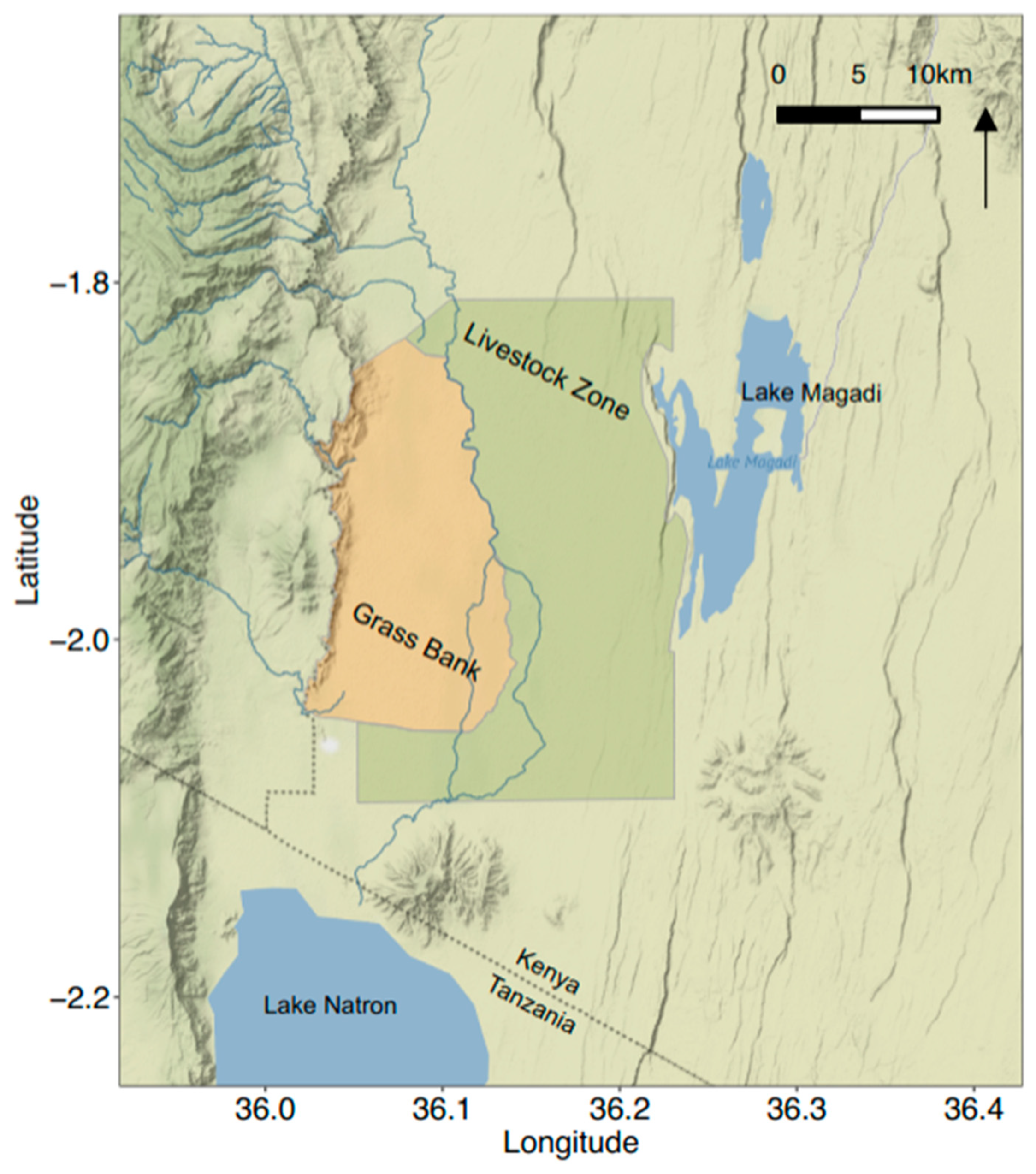
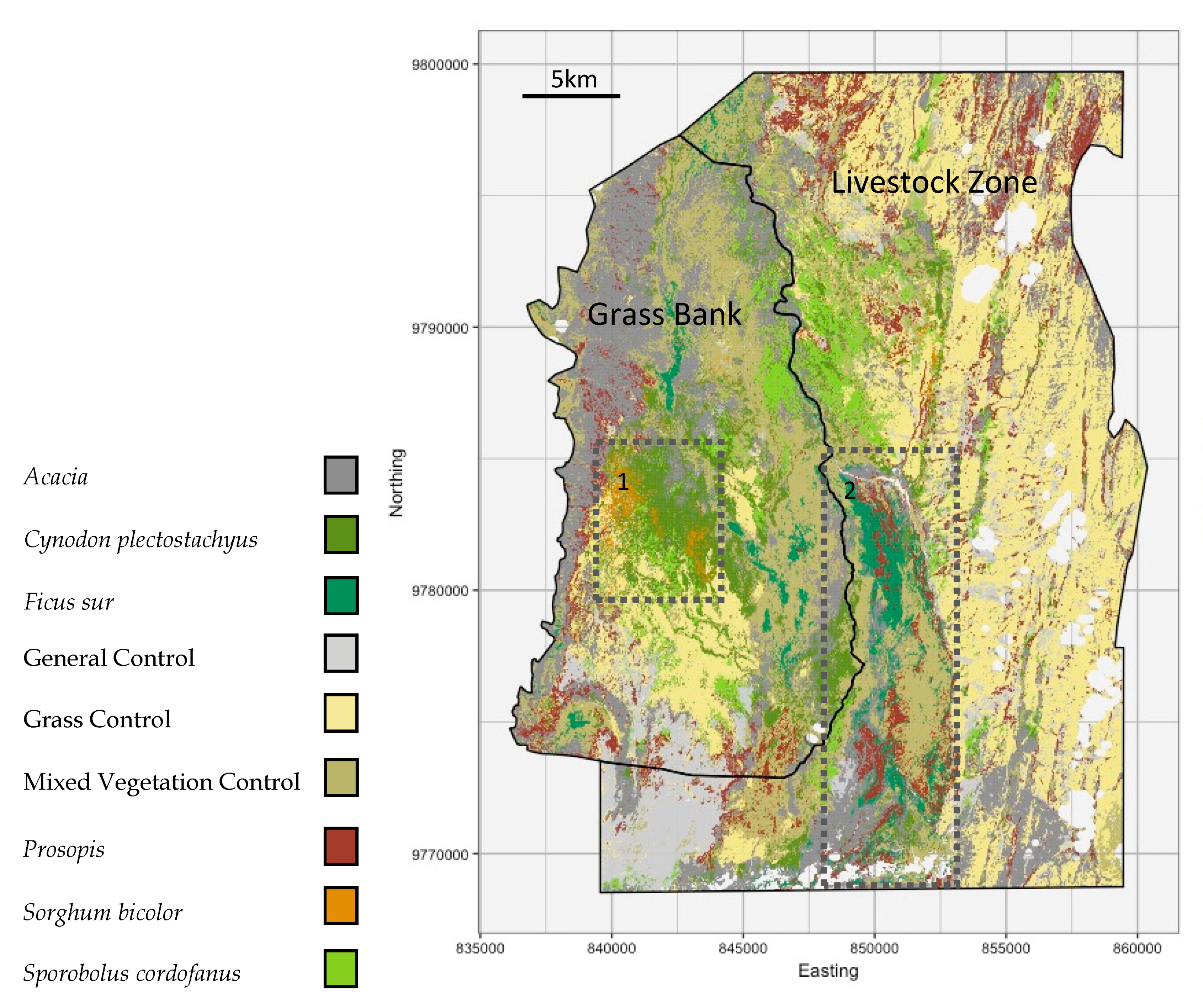
2.2. Study Area

The study area consisted of two adjacent group ranches (communally owned landholdings) in southern Kenya, namely Olkiramatian and Shompole. The ranches were characteristic of semi-arid savanna, with erratic rainfall of 400–600 mm per annum (>33% variation in annual rainfall) [39]. Rainfall was distributed bi-modally, with one long rainy season from March to May and a short rainy season in November to December. Temperatures ranged from 18 °C at night to 45 °C during the day (SORALO, unpublished data). The Olkiramatian and Shompole group ranches were bordered by the Nguruman escarpment to the east and Lake Magadi to the west, and were bisected by the perennial Ewaso Nyiro River. Grazing in both group ranches was managed by a common grazing management system. The Ewaso Nyiro River forms the boundary between two distinct grazing management areas (Figure 1); the wet season grazing area, called the Livestock Zone; and the dry season grazing area, called the Grass Bank [40]. Much of the dry season grazing area has also acted as a community-owned wildlife conservancy since the early 2000s. The conservancy contains a full assemblage of large mammals, with the exception of black rhino (Diceros bicornis) [41].
The communities living in the group ranches were predominantly Loodokilani Maasai, who seasonally move their livestock and settlements between the livestock zone in the wet season and the grass bank in the dry season and during droughts [42], thereby exploiting grazing heterogeneity by tracking the gradient of low-biomass high-quality foraging in the east to high-biomass low-quality grazing on the west [40]. Many herbivores including Grant’s gazelle (Nanger granti), impala (Aepyceros melampus), white-bearded wildebeest (Connochaetes taurinus) and zebra (Equus quagga) follow a similar seasonal grazing pattern [43]. The seasonal grazing behavior of wild herbivores is indicative of an ecologically sensible grazing management system and highlights the difference in grazing resources that are present in the seasonal grazing areas [40,43].

2.3. Field Data Collection

Ground reference data were collected by resource assessment field staff from the South Rift Association of Land Owners (SORALO). Ground reference data were collected between March and June 2019. Species (Table 1) were identified [44] and locations were presumed unchanged from the 2018 growing season, as species compositional turnover is unlikely during low rainfall [45]. Locations were identified where each of the focal vegetation species (except Ficus sur) was dominant (>80% coverage) and covered an area greater than 20 × 20 m (the coarsest spatial resolution of utilized spectral bands). GPS (Garmin eTrex 10) was used to plot the coordinates of the center of each plot. For all focal species, the target sample size was between 50 and 150 GPS points. In order to avoid constraining the classification to one of six classes, data for several control classes were also collected. For each of the control classes the target sample size was between 50 and 150 GPS points and control classes were divided into grass control (mixed grass species), mixed vegetation control (mixed species/vegetation type) and general control (bare earth/rock/sparse vegetation). The accuracy of the GPS points was assessed by collecting points in the same location several times within a time interval of 20 min. From this, average distance and standard deviation between points taken at the same location were calculated.
Data for fig trees were collected remotely using high resolution (<2 m) GEI from 2017 or later, with an overlaid Sentinel-2 scene. The overlaid S2 scene was used to avoid collecting data in areas where fig trees had been removed/died since GEI acquisition. The identification of areas of sufficiently large and dense fig coverage was verified by experts familiar with the landscape. Some grass control and mixed vegetation control data were also collected by GEI, using data from June 2018 pertaining to the species composition of distinct sampling points (SORALO unpublished data) [8].

2.4. Image Processing and Band Selection

Sentinel-2 images from across the wet season (March–May 2018) and dry season (June–October 2018) with less than 10% cloud cover were assessed for suitability. The selected images were downloaded and radiometrically corrected from level-1C (top of atmosphere product) to level-2A (bottom of atmosphere product) using the Sen2core processor version 02.05.05 [47].
Cloudy pixels were identified using the Fmask, which was originally developed for Landsat imagery [48]. The Fmask is considered an advancement on the level-1 and Sen2core cloud masks [49]. The Fmask also detects pixels covered by water, and consequently the Fmask was used to detect cloud and water for each image, with both masked from analysis.
Level-2A images containing the bands shown in Table 2 were stacked, and cloud and cloud shadow masks were applied using R version 3.5.3 [50] and the Raster package [51]. Thus, for each date of image acquisition a stack of nine masked rasters was constructed, and for time series image sets the stacks of nine rasters were combined.

2.5. Classification

RF and SVM algorithms were conducted in R and implemented with the caret package [52]. The caret package was chosen for its utility in model comparison using common syntax.
RF is an ensemble classifier consisting of decision trees; it classifies by bootstrap aggregation, which results in the production of different training subsets and a diversity of trees where each tree provides a classification result for the samples not chosen. Optimizing hyperparameters for RF using the randomForest package [53] and caret package syntax is relatively simple given that there are only two hyperparameters: (1) the number of decision trees, and (2) the number of random variables available at each node (mtry). Accuracy tends to increase with additional decision trees but plateaus after a point. A value of 500 is generally considered to be more than sufficient to reach this plateau when using small reference data with few classes (<10) and small sample sizes (<200) [54]. Optimizing the number of random variables is also relatively simple, with values ranging from 1 to the number of predictor variables (which in this case is the number of bands multiplied by the number of images used in the data set) [54].
The SVM algorithm classifies data by constructing a hyperplane in multi-dimensional feature space that maximally separates the training samples of different classes. SVM requires optimization of the hyperparameters cost (c) and kernel type (linear or radial) [55]. Studies investigating the effect of parameter optimization of SVM for application in remote sensing are contradictory [16]. Some studies report no significant improvement of accuracy with parameter optimization [56], while others report large improvements [16]. Of studies showing significant effects, choice of kernel (linear or radial) have had the largest effect on accuracy [20,57]. A such, we chose to produce SVM models with linear and radial kernels.
Optimization of hyperparameters was conducted using a manual grid containing combinations of values to test. Model accuracy statistics were obtained using 10 repetitions of the 3-fold cross-validation method. The validation method works by division of the reference data set, where each data set has a corresponding set of held-out samples. For all combinations of hyperparameter values, the model was fit to each of the data subsets and the model was used to predict the held-out samples. Performance is estimated by aggregation of model validation results from the held-out samples [58]. These performance estimates can then be used to evaluate which hyperparameter values should be used to optimize classification. Only three folds were conducted due to the small number of samples per class; this method has been employed in similar studies with small reference data sets [20].
Three image sets were created on which RF, SVM linear kernel and SVM radial kernel classifications were conducted. The number of images included in each of the three predictor data sets is outlined below. Each image contains nine bands (Table 2).
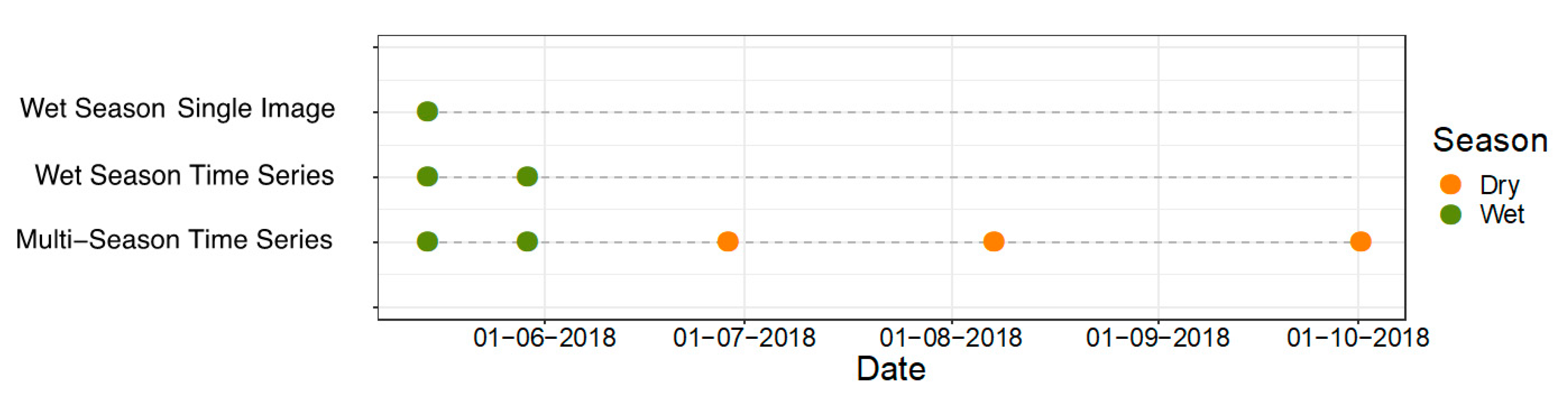
  • Wet Season Single Image—one image wet season
  • Wet Season Time Series—two images wet season
  • Multi-Season Time Series—two images wet season, three images dry season
Models with optimized hyperparameters were replicated 100 times to obtain mean and standard deviation values for model accuracy statistics. Models were trained using 70% of the samples from each class, samples were selected at random each time the model was run and predictors were scaled and centered prior to classification. Confusion matrices were produced for each of the replicates using the remaining 30% of samples in each class. Classification maps were produced by taking the most frequently occurring value at any one pixel from across the 100 classification model predictions. R code, reference data and other methodological details can be found in the link provided in the supplementary material.

3. Results

3.1. Reference Data

For the majority of classes, more than 50 samples were collected (Table 3). Few areas larger than 20 × 20 m and with high density were identified for Prosopis and Sorghum bicolor, which limited model training for these classes.
The assessment of GPS accuracy revealed that point accuracy varied by mean = 5.343 m and SD = 0.467 m. Consequently, values were only extracted from pixels containing the ground reference GPS point for model training. The point and associated pixel were assumed to correspond to the most accurate reflectance values of the class, regardless of the point’s position within the pixel area.

3.2. Image Selection

In total, five images were selected for inclusion in this study (Figure 2). Two images were obtained over the rainy season and three images over the dry season. All wet season images were obtained from mid to late May because this was the only period where cloud coverage did not significantly obscure the study area. The three dry season images were collected with approximate equidistance from each other.

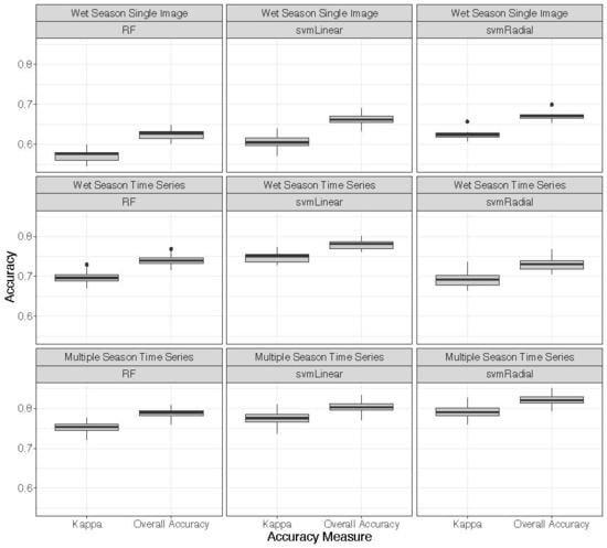
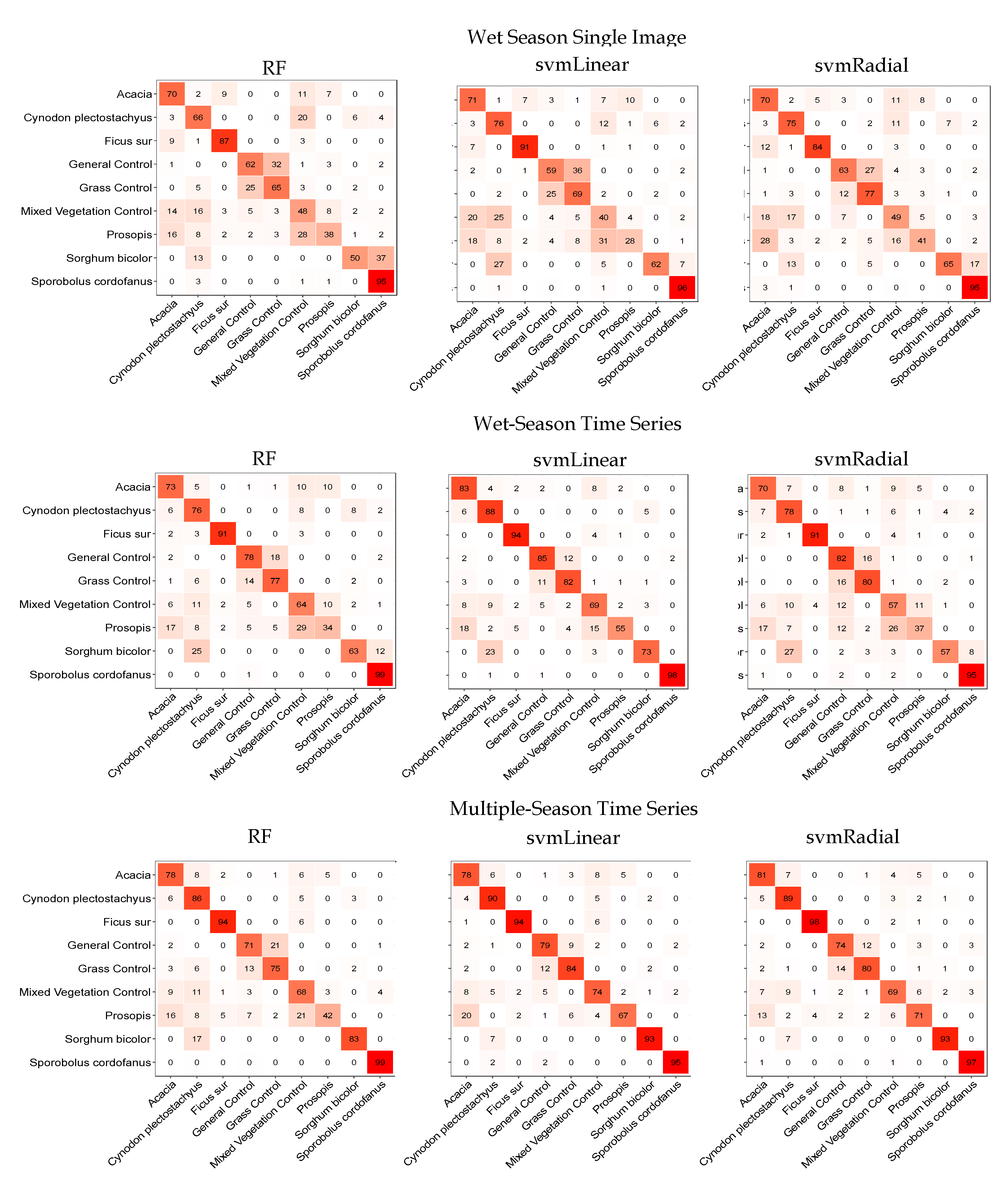
3.3. Classifications

For the RF and svmLinear models, optimal values for mtry and Cost declined with increasing image sets. In contrast, optimized svmRadial values for both Cost and Sigma were stable across all image sets (Table 4).
Models were assessed using overall accuracy (OA) and Kappa coefficients. The OA coefficient, expressed as a percentage, represents the probability that a pixel is correctly classified. The Kappa coefficient shows how much better the classifier is compared to expected its accuracy (i.e., random chance). Higher Kappa values represent more-accurate classifications [57]. Kappa coefficients are a more reliable estimate of model accuracy when class sample sizes vary widely [34]. The model with the greatest accuracy according to mean OA and Kappa coefficients was svmRadial, with the multiple-season time series image set (Figure 3), which marginally out-performed the svmLinear multiple-season time series image set in mean OA and Kappa coefficients (svmRadial mean OA = 0.8217, SD = 0.0118; mean Kappa = 0.7923, SD = 0.0135; svmLinear mean OA = 0.803, SD = 0.0135; mean Kappa = 0.7758, SD = 0.0117).
Confusion matrices were produced from the mean entries from 100 model replicates and normalized to show percentages to make classes directly comparable [59]. Normalizing confusion matrices is a common practice in assessing classification map accuracies, but tends to bias user accuracy (UA) and producer accuracy (PA) statistics if sample sizes vary considerably between classes (see Table 3 for class sample sizes). As a consequence of an unbalanced training data set, these statistics were not calculated, and the confusion matrices alone demonstrate class accuracy trends across classifiers and image sets (Figure 4) [60].
Figure 5 and Figure 6 show that the grass bank (dry season grazing area) and the livestock zone (wet season grazing areas) varied in the spatial distribution and proportional cover of the focal species and control classes. The grass bank was dominated by mixed vegetation types (trees, shrubs, grass/forbs) and contained large areas of the taller perennial grass Cynodon plectostachyus (Figure 5 and Figure 6). Additionally, the grass bank contained the vast majority of the perennial Sorghum bicolor found in the study area (Figure 5 and Figure 6). The livestock zone (wet season grazing area) contained large proportions of general control (bare earth and sparse vegetation), grass control (areas dominated by grass but not the focal grass species), mixed vegetation and the invasive shrub Prosopis (Figure 5 and Figure 6). The two grazing areas contained similar proportions of Acacia and Sporobolus cordofanus, and the majority of S. cordofanus was contained within a single continuous zone that spanned both grazing areas (Figure 5 and Figure 6).

4. Discussion

4.1. Classifications

This study successfully demonstrates the utility of using multi-season time-series imagery for classifying focal species with high classification accuracy (OA = 0.8217, Kappa = 0.7923). Increasing the number of images and including dry season imagery results in more-accurate classification, regardless of classifier (mean increase in OA = 0.1641, Figure 3). These results indicate that open-access multi-spectral imagery (e.g., Sentinel-2 imagery) has the potential to discriminate between highly similar land cover types and produce accurate and class-rich classification maps. This is likely to be applicable to the production of classification maps across a range of biophysical land cover types that vary in their spectral signatures over time. Improving classification maps of Earth’s biophysical cover is key to data-driven environmental monitoring and natural resource management [61].
The svmRadial classifier with multi-season time-series image sets resulted in the highest OA and Kappa values, and RF consistently produced the lowest OA and Kappa values regardless of image set. The svmRadial and svmLinear classifiers generally produced similar results except with the wet season time series image set, where svmRadial under-performed compared to svmLinear (Figure 3). A large increase in accuracy was expected with the inclusion of multiple images acquired in the wet season; however, unexpected increases in accuracy of a similar size were found when using time series imagery with dry season images (single-image wet season mean OA for all models was >63; time series wet season mean OA for all models was >74; time series multiple season mean OA for all models was >79). These accuracies are comparable to studies using expensive airborne hyperspectral and high spatial resolution imagery to classify plant species and vegetation types [30,34,62,63,64,65]. The narrow bandwidth red edge bands (bands 5, 6 and 7) provided by the MSI on Sentinel-2 are comparable to bands found on hyperspectral instruments, which likely facilitated the spectral separation of plant species [66]. Time-series imagery from Sentinel-2 appears to change classification accuracy in ways comparable to the use of single images obtained from hyperspectral and high spatial resolution instruments.
Rapinel at al. (2019) [20] compared the accuracy of classifying grasses with RF, svmLinear and svmRadial using Sentinel-2 images taken at various dates across a year as well as using a time series image set containing all images from all dates (12 total). They found that the most accurate classification was obtained using time series imagery, and that svmLinear out-performed svmRadial and RF (marginally for svmRadial). The present study is generally in agreement with Rapinel et al. (2019) [20], and goes one step further to demonstrate that the inclusion of time series season imagery from within a season (the growth season) increases classification accuracy, although to a lesser extent than when classification is performed on time series imagery that includes images from across seasons (growth and dry seasons). Increasing image numbers in a time series image set is known to increase classification accuracy for plant species [34]. The time series data set used in Schuster et al., (2015) [34] were stacked from the first date of image acquisition onwards, increasing by one image for each image set, and accuracy plateaued after approximately four images. This means it was not possible to show the effect of season on accuracy, as accuracy had plateaued before the end of the growing season. One limitation of the current study is that further time series image sets with greater numbers of images are required to quantify the number of images at which accuracy plateaus. However, it is unlikely that the inclusion of further dry season images would result in an increase in accuracy of comparative size [34].
The confusion matrices show a complex relationship between image sets and accuracy. The majority of classes increased their accuracy with respect to increasing image numbers and with the inclusion of dry season imagery, regardless of classifier. S. cordofanus was an exception, with very high classification accuracy across all models and image sets (Figure 4). For all classifiers, the general control class (bare soil and/or sparse vegetation) had reduced accuracy of at least 6% with the multi-season time series image set compared with the wet season time series image set. The misclassification of grass control and general control for models containing dry season imagery (Figure 4) was expected, as areas turn from grass-dominated to bare earth or sparse vegetation as the dry season progresses. This means that the two classes displayed similar dry season spectral characteristics.
Class accuracy order was generally preserved across all confusion matrices. S. cordofanus was consistently classified with the highest accuracy (maximum = 99%, minimum = 95%), and Prosopis was consistently classified with the lowest accuracy and was most commonly misclassified as Acacia (maximum = 71%, minimum = 28%, Figure 4). Prosopis, an invasive shrub, has a particularly deep taproot that allows the plant to remain unusually green into the dry season [67]. This characteristic was expected to result in high classification accuracy in models including dry season imagery, but the results are in clear contrast with this prediction (Figure 4). Misclassification of Prosopis is likely to have been a consequence of poor availability of ground reference sites, and a lack of large contiguous patches of Prosopis. The accuracy of woody and grass species did not differ in their response to the inclusion of dry season imagery in classifications (Figure 5). This finding is surprising because it indicates that the dry season spectral characteristics of grasses remain sufficiently distinct to enhance classification accuracy despite browning and consumption by herbivores, which occurs rapidly in the study area [40].

4.2. Classification Maps and Grazing

Classification maps demonstrate that the coverage and spatial distribution of classes in the grazing areas varied substantially, and therefore that the habitat and grazing opportunities that the areas provided differed (Figure 4 and Figure 5). Such heterogeneity in species composition (and their functional traits) is an essential characteristic of landscapes that support a diverse assemblage of large herbivores [5,9,68]. Crucially, the large areas of grass control in the livestock zone (that are predominately but not exclusively dominated by annuals), coupled with large areas of S. cordofanus, are suitable for grazing in the wet season due to the low biomass but high nutritional content of these areas [8,40]. In Figure 5, two areas with distinct vegetation characteristics are highlighted. Area 1 contained most of the S. bicolor coverage in the study area and a high density of C. plectostachyus, a highly nutritious and high biomass grass (SORALO, unpublished data). Both grass species served to buffer grazing herbivores through dry seasons and drought, and their distributions were considerably restricted to the grass bank grazing area (Figure 5). Area 2 contained the Ewaso Nyiro Swamp, which is dominated by fig forest, mixed vegetation, and large patches of Prosopis (Figure 5). The swamp is generally grazed in the dry season, but is particularly import for grazing wildlife and livestock during droughts when the remaining buffer resources in area 1 are depleted by both livestock and wildlife. Grazing in the swamp is threatened by encroaching patches of the invasive Prosopis shrub, which excludes native vegetation (especially in areas of higher soil moisture), and therefore green late season forage such as that found in the swap. Maintaining livestock and wild herbivore access to grazing resources such as those in areas 1 and 2 is crucial to sustaining populations, pastoralist livelihoods and conservation efforts, particularly in light of increasingly prolonged and severe dry seasons [40,43,69].

4.3. Limitations

This study was limited by a lack of sufficiently cloud-free imagery available across the wet season and, as a result, was unable to investigate the relative importance of imagery obtained at the start and middle of the growing season. Earth observation satellites with more frequent revisit time (one to two days) but lower spatial resolution, such as imagery from the Moderate Resolution Imaging Spectroradiometer (MODIS) on NASA’s Terra and Aqua Satellites, have the potential to build cloud-free composites of the missing time frame [70]. However, the spatial resolution of MODIS (minimum spatial resolution = 250 m) is incompatible with the small, patchy nature of the focal species, and therefore pixel level reflectance values from MODIS imagery extracted at GPS training data points are unlikely to be representative of the training data class. Consequently, MODIS and other moderate resolution satellite imagery were not used to compensate for the lack of early growth season imagery from Sentinel-2. Another solution to the problem of cloud cover is to use imagery obtained from unmanned aerial vehicles (UAVs) or aircraft below cloud level. Sensors on these platforms have high spatial resolution but limited coverage. Imagery from these platforms can be used to produce classification maps of plant species, although accuracies depend on sensor characteristics [71]. For this study, a multi-platform approach was ruled out due to logistical and cost issues, and because of the difficulties in combining imagery from different platforms, sensors and time frames [72]. Further, the use of multi-spectral satellite imagery for mapping plant species was considered the priority research question. Despite issues with cloud cover, the classification accuracies obtained were sufficient to produce accurate maps of species distribution and demonstrate that just two relatively cloud-free images per growth season are sufficient to produce accurate maps (Figure 3 and Figure 4).

5. Conclusions

This study highlighted the utility of multi-spectral satellite imagery for producing species-level maps at a landscape scale. It also illustrated the positive effect time series imagery can have on classification accuracy. In addition to image sets, accurate classification and mapping of species with Sentinel-2 appeared to depend on the species being mapped and the classifier. Our study area, and savannas across Africa, are changing significantly, and in many regions savannas are experiencing continual degradation and losses in productivity. The techniques used in this study provide an important methodological base for savanna assessment and monitoring across large scales at a low cost. Importantly, our method uses freely distributed imagery and software that can be integrated into existing data platforms for land managers and key decision makers [73].

Supplementary Materials

The following are available online at https://0-www-mdpi-com.brum.beds.ac.uk/2072-4292/12/1/198/s1. Access to ground reference data can be obtained at the following doi:10.5281/zenodo.3538339 (https://zenodo.org/record/3538339#.XcnV9TKwlhE). Code and other methodological details can be found at the following doi:10.5281/zenodo.3563030 (https://zenodo.org/record/3563030#.XegDljKwkWo).

Author Contributions

F.D.L.H., E.T.A.M., P.T. and S.R. were involved in the conceptualization of the study and methodology; formal analysis, F.D.L.H.; data curation, F.D.L.H. and S.R.; writing—original draft preparation, F.D.L.H.; writing—review and editing, F.D.L.H., E.T.A.M., P.T. and S.R.; visualization, F.D.L.H.; supervision, E.T.A.M.; project administration, F.D.L.H., S.R. All authors have read and agreed to the published version of the manuscript.

Funding

This research was funded by the UKRI Natural Environment Research Council (NERC) grant ‘SEOSAW’ to the University of Edinburgh (grant ref NE/P008755/1).

Acknowledgments

The authors would like to thank Guy Western and John Kamanga for their support of the project, and to Joel Meja Sumare and the rest of the team at the Lale’enok Resource Centre for their efforts in the field.

Conflicts of Interest

The authors declare no conflict of interest.

References

  1. Scholes, R.J.; Walker, B.H. An African Savanna: Synthesis of the Nylsvley Study; Cambridge University Press: Cambridge, UK, 2004. [Google Scholar]
  2. Cassidy, L.; Fynn, R.; Sethebe, B. Effects of restriction of wild herbivore movement on woody and herbaceous vegetation in the Okavango Delta Botswana. Afr. J. Ecol. 2013, 51, 513–527. [Google Scholar] [CrossRef]
  3. McCleery, R.; Monadjem, A.; Baiser, B.; Fletcher, R., Jr.; Vickers, K.; Kruger, L. Animal diversity declines with broad-scale homogenization of canopy cover in African savannas. Biol. Conserv. 2018, 226, 54–62. [Google Scholar] [CrossRef]
  4. Western, D. The environment and ecology of pastoralists in arid savannas. Dev. Chang. 1982, 13, 183–211. [Google Scholar] [CrossRef]
  5. Owen-Smith, N. Functional heterogeneity in resources within landscapes and herbivore population dynamics. Landsc. Ecol. 2004, 19, 761–771. [Google Scholar] [CrossRef]
  6. Owen-Smith, R.N. Adaptive Herbivore Ecology: From Resources to Populations in Variable Environments; Cambridge University Press: Cambridge, UK, 2002. [Google Scholar]
  7. Illius, A.W.; O’connor, T.G. Resource heterogeneity and ungulate population dynamics. Oikos 2000, 89, 283–294. [Google Scholar] [CrossRef] [Green Version]
  8. Hunter, F.; Tyrrell, P.D.; Breahony, P.; Nyange, M.; Russell, S. Maintaining Functional Heterogeneity at the LivestockWildlife Interface: The Role of Floral Species Composition. J. Rangel. Ecol. Manag. submitted.
  9. Fuhlendorf, S.D.; Fynn, R.W.; McGranahan, D.A.; Twidwell, D. Heterogeneity as the basis for rangeland management. In Rangelan Systems; Springer: Cham, Germany, 2017; pp. 169–196. [Google Scholar] [CrossRef] [Green Version]
  10. Higgins, S.I.; Shackleton, C.M.; Robinson, E.R. Changes in woody community structure and composition under constrasting landuse systems in a semi-arid savanna, South Africa. J. Biogeogr. 1999, 26, 619–627. [Google Scholar] [CrossRef]
  11. Groom, R.J.; Western, D. Impact of land subdivision and sedentarization on wildlife in Kenya’s southern rangelands. Rangel. Ecol. Manag. 2013, 66, 1–9. [Google Scholar] [CrossRef]
  12. Western, D.; Groom, R.; Worden, J. The impact of subdivision and sedentarization of pastoral lands on wildlife in an African savanna ecosystem. Biol. Conserv. 2009, 142, 2538–2546. [Google Scholar] [CrossRef]
  13. Schmidt, K.S.; Skidmore, A.K. Spectral discrimination of vegetation types in a coastal wetland. Remote Sens. Environ. 2003, 85, 92–108. [Google Scholar] [CrossRef]
  14. Sianga, K.; Fynn, R. The vegetation and wildlife habitats of the Savuti-Mababe-Linyanti ecosystem, northern Botswana. Koedoe 2017, 59, 1–16. [Google Scholar] [CrossRef] [Green Version]
  15. Lillesand, T.; Kiefer, R.W.; Chipman, J. Remote Sensing and Image Interpretation; John Wiley & Sons: Hoboken, NJ, USA, 2014. [Google Scholar]
  16. Maxwell, A.E.; Warner, T.A.; Fang, F. Implementation of machine-learning classification remote sensing: An applied review. Int. J. Remote Sens. 2018, 39, 2784–2817. [Google Scholar] [CrossRef] [Green Version]
  17. Belgiu, M.; Drăguţ, L. Random forest in remote sensing: A review of applications and future directions. ISPRS J. Photogramm. Remote Sens. 2016, 114, 24–31. [Google Scholar] [CrossRef]
  18. Mansour, K.; Mutanga, O.; Adam, E.; Abdel-Rahman, E.M. Multispectral remote sensing for mapping grassland degradation using the key indicators of grass species and edaphic factors. Geocarto Int. 2016, 31, 477–491. [Google Scholar] [CrossRef]
  19. Xie, Y.; Sha, Z.; Yu, M. Remote sensing imagery in vegetation mapping: A review. J. Plant Ecol. 2008, 1, 9–23. [Google Scholar] [CrossRef]
  20. Rapinel, S.; Mony, C.; Lecoq, L.; Clément, B.; Thomas, A.; Hubert-Moy, L. Evaluation of Sentinel-2 time-series for mapping floodplain grassland plant communities. Remote Sens. Environ. 2017, 223, 115–129. [Google Scholar] [CrossRef]
  21. Bishop, C.M. Pattern Recognition and Machine Learning; Springer: Berlin/Heidelberg, Germany, 2006. [Google Scholar] [CrossRef]
  22. Montgomery, D.C.; Peck, E.A.; Vining, G.G. Introduction to Linear Regression Analysis (Vol. 821); John Wiley & Sons: Hoboken, NJ, USA, 2012. [Google Scholar] [CrossRef]
  23. Adam, E.; Mutanga, O.; Odindi, J.; Abdel-Rahman, E.M. Land-use/cover classification in a heterogeneous coastal landscape using RapidEye imagery: Evaluating the performance of random forest and support vector machines classifiers. Int. J. Remote Sens. 2014, 35, 3440–3458. [Google Scholar] [CrossRef]
  24. Fethers, J. Remote Sensing of Eelgrass using Object Based Image Analysis and Sentinel-2 Imagery. Master’s Thesis, University of Allborg, Aalborg, Denmark, 2017. [Google Scholar]
  25. Liu, P.; Choo, K.K.R.; Wang, L.; Huang, F. SVM or deep learning? A comparative study on remote sensing image classification. Soft Comput. 2017, 21, 7053–7065. [Google Scholar] [CrossRef]
  26. Mashamba, T. Mapping Grass Nutrient Phosphorus (P) and Sodium (NA) across Different Grass Communities Using Sentinel-2 Data. Master’s Thesis, University of the Witwatersrand, Johannesburg, South Africa, 2017. [Google Scholar]
  27. Raczko, E.; Zagajewski, B. Comparison of support vector machine, random forest and neural network classifiers for tree species classification on airborne hyperspectral APEX images. Eur. J. Remote Sens. 2017, 50, 144–154. [Google Scholar] [CrossRef] [Green Version]
  28. Skidmore, A.K.; Forbes, G.W.; Carpenter, D.J. Technical note non-parametric test of overlap in multispectral classification. Remote Sens. 1988, 9, 777–785. [Google Scholar] [CrossRef]
  29. Castro-Esau, K.L.; Sánchez-Azofeifa, G.A.; Rivard, B.; Wright, S.J.; Quesada, M. Variability in leaf optical properties of Mesoamerican trees and the potential for species classification. Am. J. Bot. 2006, 93, 517–530. [Google Scholar] [CrossRef]
  30. Feilhauer, H.; Thonfeld, F.; Faude, U.; He, K.S.; Rocchini, D.; Schmidtlein, S. Assessing floristic composition with multispectral sensors—A comparison based on monotemporal and multiseasonal field spectra. Int. J. Appl. Earth Obs. Geoinf. 2013, 21, 218–229. [Google Scholar] [CrossRef]
  31. Fassnacht, F.E.; Latifi, H.; Stereńczak, K.; Modzelewska, A.; Lefsky, M.; Waser, L.T.; Straub, C.; Ghosh, A. Review of studies on tree species classification from remotely sensed data. Remote Sens. Environ. 2016, 186, 64–87. [Google Scholar] [CrossRef]
  32. Shoko, C.; Mutanga, O. Examining the strength of the newly-launched Sentinel 2 MSI sensor in detecting and discriminating subtle differences between C3 and C4 grass species. ISPRS J. Photogramm. Remote Sens. 2017, 129, 32–40. [Google Scholar] [CrossRef]
  33. Miyoshi, G.T.; Imai, N.N.; De Moraes, M.V.A.; Tommaselli, A.M.G.; Näsi, R. Time series of images to improve tree species classification. Int. Arch. Photogramm. Remote Sens. Spat. Inf. Sci. 2017, 42. [Google Scholar] [CrossRef] [Green Version]
  34. Schuster, C.; Schmidt, T.; Conrad, C.; Kleinschmit, B.; Förster, M. Grassland habitat mapping by intra-annual time series analysis–Comparison of RapidEye and TerraSAR-X satellite data. Int. J. Appl. Earth Obs. Geoinf. 2015, 34, 25–34. [Google Scholar] [CrossRef]
  35. Mitchard, E.T.; Flintrop, C.M. Woody encroachment and forest degradation in sub-Saharan Africa’s woodlands and savannas 1982–2006. Philos. Trans. R. Soc. B Biol. Sci. 2013, 368, 20120406. [Google Scholar] [CrossRef] [Green Version]
  36. Drusch, M.; Del Bello, U.; Carlier, S.; Colin, O.; Fernandez, V.; Gascon, F.; Hoersch, B.; Isola, C.; Laberinti, P.; Martimort, P.; et al. Sentinel-2: ESA’s optical high-resolution mission for GMES operational services. Remote Sens. Environ. 2012, 120, 25–36. [Google Scholar] [CrossRef]
  37. Ntiati, P. Group Ranch Subdivision Study in Loitokitok Division of Kajiado District, Kenya; Lucid Working Paper Series No. 7, Lucid; LUCID Project; International Livestock Research Institute: Nairobi, Kenya, 2002. [Google Scholar]
  38. Mwangi, M.N.; Desanker, P.V. Changing climate, disrupted livelihoods: The case of vulnerability of nomadic Maasai pastoralism to recurrent droughts in Kajiado District, Kenya. In Proceedings of the American Geophysical Union, Fall Meeting 2007, San Francisco, CA, USA, 10–14 December 2007. abstract id. GC12A-02. [Google Scholar]
  39. Agnew, A.D.Q.; Mwendia, C.M.; Oloo, G.O.; Roderick, S.; Stevenson, P. Landscape monitoring of semi-arid rangelands in the Kenyan Rift Valley. Afr. J. Ecol. 2000, 38, 277–285. [Google Scholar] [CrossRef]
  40. Russell, S.; Tyrrell, P.; Western, D. Seasonal interactions of pastoralists and wildlife in relation to pasture in an African savanna ecosystem. J. Arid Environ. 2018, 154, 70–81. [Google Scholar] [CrossRef]
  41. Schuette, P.; Creel, S.; Christianson, D. Coexistence of African lions, livestock, and people in a landscape with variable human land use and seasonal movements. Biol. Conserv. 2013, 157, 148–154. [Google Scholar] [CrossRef] [Green Version]
  42. Western, G. Conflict or Coexistence. Ph.D. Thesis, University of Oxford, Oxford, UK, 2018. [Google Scholar]
  43. Tyrrell, P.; Russell, S.; Western, D. Seasonal movements of wildlife and livestock in a heterogenous pastoral landscape: Implications for coexistence and community based conservation. Glob. Ecol. Conserv. 2017, 12, 59–72. [Google Scholar] [CrossRef]
  44. Dharani, N. Field Guide to Common Trees & Shrubs of East Africa; Penguin Random House: Cape Town, South Africa, 2011. [Google Scholar]
  45. Dumont, B.; Rossignol, N.; Loucougaray, G.; Carrère, P.; Chadoeuf, J.; Fleurance, G.; Bonis, A.; Farruggia, A.; Gaucherand, S.; Ginane, C.; et al. When does grazing generate stable vegetation patterns in temperate pastures? Agric. Ecosyst. Environ. 2012, 153, 50–56. [Google Scholar] [CrossRef]
  46. Dubow, A.Z. Mapping and Managing the Spread of Prosopis Juliflora in Garissa County, Kenya. Master’s Thesis, Kenyatta University, Nairobi, Kenya, 2011. [Google Scholar]
  47. Main-Knorn, M.; Pflug, B.; Louis, J.; Debaecker, V.; Müller-Wilm, U.; Gascon, F. Sen2Cor for Sentinel-2. In Image and Signal Processing for Remote Sensing; International Society for Optics and Photonics: Dresden, Germany, 2017; Volume 10427, p. 1042704. [Google Scholar] [CrossRef] [Green Version]
  48. Zhu, Z.; Woodcock, C.E. Object-based cloud and cloud shadow detection in Landsat imagery. Remote Sens. Environ. 2012, 118, 83–94. [Google Scholar] [CrossRef]
  49. Frantz, D.; Haß, E.; Uhl, A.; Stoffels, J.; Hill, J. Improvement of the Fmask algorithm for Sentinel-2 images: Separating clouds from bright surfaces based on parallax effects. Remote Sens. Environ. 2018, 215, 471–481. [Google Scholar] [CrossRef]
  50. R Core Team. R: A Language and Environment for Statistical Computing; R Foundation for Statistical Computing: Vienna, Austria, 2018; Available online: https://www.R-project.org/ (accessed on 1 June 2019).
  51. Hijmans, J. Raster: Geographic Data Analysis and Modeling. R Package Version 2.8–19. 2019. Available online: https://CRAN.R-project.org/package=raster (accessed on 1 June 2019).
  52. Kuhn, M.; Wing, J.; Weston, S.; Williams, A.; Keefer, C.; Engelhardt, A.; Cooper, T.; Mayer, Z.; Kenkel, B.; Benesty, M.; et al. Caret: Classification and Regression Training; R Package Version 6.0–84. 2019. Available online: https://cran.r-project.org/web/packages/caret/caret.pdf (accessed on 1 June 2019).
  53. Liaw, A.; Wiener, M. Classification and Regression by randomForest. R News 2002, 2, 18–22. [Google Scholar]
  54. Shi, D.; Yang, X. An assessment of algorithmic parameters affecting image classification accuracy by random forests. Photogramm. Eng. Remote Sens. 2016, 82, 407–417. [Google Scholar] [CrossRef]
  55. Cortes, C.; Vapnik, V. Support-vector networks. Mach. Learn. 1995, 20, 273–297. [Google Scholar] [CrossRef]
  56. Melgani, F.; Bruzzone, L. Classification of hyperspectral remote sensing images with support vector machines. IEEE Trans. Geosci. Remote Sens. 2004, 42, 1778–1790. [Google Scholar] [CrossRef] [Green Version]
  57. Huang, C.; Davis, L.S.; Townshend, J.R.G. An assessment of support vector machines for land cover classification. Int. J. Remote Sens. 2002, 23, 725–749. [Google Scholar] [CrossRef]
  58. Kuhn, M. Building predictive models in R using the caret package. J. Stat. Softw. 2008, 28, 1–26. [Google Scholar] [CrossRef] [Green Version]
  59. Congalton, R.G.; Green, K. Assessing the Accuracy of Remotely Sensed Data: Principles and Practices; CRC Press: New York, NY, USA, 2008. [Google Scholar]
  60. Stehman, S.V. A critical evaluation of the normalized error matrix in map accuracy assessment. Photogrammetric. Eng. Remote Sens. 2004, 70, 743–751. [Google Scholar] [CrossRef]
  61. Gomez, C.; White, J.C.; Wulder, M.A. Optical remotely sensed time series data for land cover classification: A review. ISPRS J. Photogramm. Remote Sens. 2016, 116, 55–72. [Google Scholar] [CrossRef] [Green Version]
  62. Burai, P.; Deák, B.; Valkó, O.; Tomor, T. Classification of herbaceous vegetation using airborne hyperspectral imagery. Remote Sens. 2015, 7, 2046–2066. [Google Scholar] [CrossRef] [Green Version]
  63. Neumann, C.; Weiss, G.; Schmidtlein, S.; Itzerott, S.; Lausch, A.; Doktor, D.; Brell, M. Gradient-based assessment of habitat quality for spectral ecosystem monitoring. Remote Sens. 2015, 7, 2871–2898. [Google Scholar] [CrossRef] [Green Version]
  64. Oldeland, J.; Dorigo, W.; Lieckfeld, L.; Lucieer, A.; Jürgens, N. Combining vegetation indices, constrained ordination and fuzzy classification for mapping semi-natural vegetation units from hyperspectral imagery. Remote Sens. Environ. 2010, 114, 1155–1166. [Google Scholar] [CrossRef]
  65. Lopatin, J.; Fassnacht, F.E.; Kattenborn, T.; Schmidtlein, S. Mapping plant species in mixed grassland communities using close range imaging spectroscopy. Remote Sens. Environ. 2017, 201, 12–23. [Google Scholar] [CrossRef]
  66. Meerdink, S.K. Remote Sensing of Plant Species Using Airborne Hyperspectral Visible-Shortwave Infrared and Thermal Infrared Imagery. Ph.D. Thesis, UC Santa Barbara, Santa Barbara, CA, USA, 2018. [Google Scholar]
  67. Ng, W.T.; Rima, P.; Einzmann, K.; Immitzer, M.; Atzberger, C.; Eckert, S. Assessing the Potential of Sentinel-2 and Pléiades Data for the Detection of Prosopis and Vachellia spp. in Kenya. Remote Sens. 2017, 9, 74. [Google Scholar] [CrossRef] [Green Version]
  68. Fynn, R.W.; Augustine, D.J.; Peel, M.J.; de Garine-Wichatitsky, M. Strategic management of livestock to improve biodiversity conservation in African savannahs: A conceptual basis for wildlife—Livestock coexistence. J. Appl. Ecol. 2016, 53, 388–397. [Google Scholar] [CrossRef] [Green Version]
  69. Western, D.; Mose, V.N.; Worden, J.; Maitumo, D. Predicting extreme droughts in savannah Africa: A comparison of proxy and direct measures in detecting biomass fluctuations, trends and their causes. PLoS ONE 2015, 10, e0136516. [Google Scholar] [CrossRef] [Green Version]
  70. Huete, A.; Didan, K.; Miura, T.; Rodriguez, E.P.; Gao, X.; Ferreira, L.G. Overview of the radiometric and biophysical performance of the MODIS vegetation indices. Remote Sens. Environ. 2002, 83, 195–213. [Google Scholar] [CrossRef]
  71. Baldeck, C.A.; Colgan, M.S.; Féret, J.B.; Levick, S.R.; Martin, R.E.; Asner, G.P. Landscape-scale variation in plant community composition of an African savanna from airborne species mapping. Ecol. Appl. 2014, 24, 84–93. [Google Scholar] [CrossRef] [PubMed]
  72. Puliti, S.; Saarela, S.; Gobakken, T.; Ståhl, G.; Næsset, E. Combining UAV and Sentinel-2 auxiliary data for forest growing stock volume estimation through hierarchical model-based inference. Remote Sens. Environ. 2018, 204, 485–497. [Google Scholar] [CrossRef]
  73. Mose, V.N.; Western, D.; Tyrrell, P. Application of open source tools for biodiversity conservation and natural resource management in East Africa. Ecol. Inform. 2018, 47, 35–44. [Google Scholar] [CrossRef]
Figure 1. Map of the study area showing the livestock zone and grass bank grazing areas.
Remotesensing 12 00198 g001
Figure 2. Timeline of image acquisition. The combination of images used for each of the three image sets is also shown.
Remotesensing 12 00198 g002
Figure 3. The effect of classifier and image sets on Overall Accuracy (OA) and Kappa coefficients. Distributions of accuracy coefficients were obtained from 100 replicates.
Remotesensing 12 00198 g003
Figure 4. Normalized confusion matrix values for all combinations of classifier and image set. Entries are the percentages of average cell counts from 100 model replicates. A low white to high red color scale was applied to facilitate interpretation.
Remotesensing 12 00198 g004
Figure 5. Classification map for the most accurate model (svmRadial with a time series multiple season image set) showing the spatial distribution of classes across the seasonal grazing areas. The most frequent class assigned to a pixel from 100 classification replicates was used as the final mapped pixel value. Important regions of the study area for grazing and sustainability are highlighted by boxes 1 and 2, and white areas are those masked by cloud cover.
Remotesensing 12 00198 g005
Figure 6. Mean pixel counts of each class as a percentage cover of the grass bank and livestock zone seasonal grazing areas. Values are calculated from 100 replicates of the svmRadial classifier with image sets of multiple-season time series. Standard deviation error bars are present but are visibly negligible.
Remotesensing 12 00198 g006
Table 1. The focal species, reasons for mapping and key characteristics.
SpeciesCharacteristics
Acacia spp.A genus of trees adapted to arid and semi-arid environments. Known to have proliferated in the area over the last 50 years. Increased density of Acacia trees is an indicator of land degradation, resulting in reduced grazing quality.
Cynodon plectostachyusA perennial grass identified by local pastoralists in group discussions as one of the top 10 most important grazing species in both wet and dry seasons due to its fast growth, high nutritional content and high biomass [8]. This species occurs at high density, but stands may also contain some other species at a low abundance.
Ficus surThese fig trees are large and occur in clusters with dense tree crowns that can be identified remotely with recent Google Earth imagery (GEI). Fig trees are thought to be declining in the area and provide foraging resources and habitat to several primate species, including the endangered black and white colobus monkey (Colobus guereza).
Prosopis (juliflora, pallida and hybrids)An invasive shrub and a major threat to communal rangelands in East Africa through its capacity to out-compete native species [46]. Remains green long into the dry season due to an unusually deep taproot.
Sorghum bicolorCritically important high biomass perennial grazing resource that buffers herbivore populations through droughts. Occurs in discrete and dense patches.
Sporobolus cordofanusIdentified by local pastoralists in group discussions as one of the top 10 most important grazing species during the wet season. The species is annual and the most abundant grass in the region, dominating many grass plains [8].
Table 2. Sentinel-2 spectral bands utilized in this study [36]. Bands with 10-m resolution were resampled to 20-m resolution during Sen2cor processing to maintain spatial resolution consistency across bands.
 BandCentral Wavelength (nm)Band Width (nm)Spatial Resolution (m)
 Band 2—Blue492.46610
 Band 3—Green559.83610
 Band 4—Red664.63110
 Band 5—Red edge704.11520
 Band 6—Red edge740.51520
 Band 7—Red edge782.82020
 Band 8A Narrow NIR864.72120
 Band 11 SWIR1613.79120
 Band 12 SWIR2202.417520
Table 3. Summary of sample sizes for each class of ground reference data.
ClassNo. Samples
Acacia78
Cynodon plectostachyus71
Ficus sur55
General Control64
Grass Control150
Mixed Vegetation Control93
Prosopis45
Sorghum bicolor20
Sporobolus cordofanus99
Table 4. Hyperparameter values used in 100 replicates for each Random Forest (RF) and Support Vector Machine (SVM) model, with values obtained from repeated k-fold validation with a manual grid.
ModelImage SetHyperparameter Values
RFWet season single imageNumber of trees = 500, mtry = 5
svmLinearWet season single imageCost = 15
svmRadialWet season single imageCost = 25, Sigma = 0.1
RFWet season time seriesNumber of trees = 500, mtry = 4
svmLinearWet season time seriesCost = 7
svmRadialWet season time seriesCost = 25, Sigma = 0.1
RFMultiple-season time seriesNumber of trees = 500, mtry = 3
svmLinearMultiple-season time seriesCost = 2
svmRadialMultiple-season time seriesCost = 25, Sigma = 0.1

