Article

Accurate Despeckling and Estimation of Polarimetric Features by Means of a Spatial Decorrelation of the Noise in Complex PolSAR Data

by
Alberto Arienzo
1,2,
Fabrizio Argenti
1,
Luciano Alparone
1,* and
Monica Gherardelli
1
1
Department of Information Engineering, University of Florence, 50139 Florence, Italy
2
Institute of Applied Physics “Nello Carrara”, Research Area of Florence, 50019 Sesto Fiorentino (FI), Italy
*
Author to whom correspondence should be addressed.
Submission received: 4 December 2019 / Revised: 9 January 2020 / Accepted: 11 January 2020 / Published: 20 January 2020

Abstract

:
In this work, we extended a procedure for the spatial decorrelation of fully-developed speckle, originally developed for single-polarization SAR data, to fully-polarimetric SAR data. The spatial correlation of the noise depends on the tapering window in the Fourier domain used by the SAR processor to avoid defocusing of targets caused by Gibbs effects. Since each polarimetric channel is focused independently of the others, the noise-whitening procedure can be performed applying the decorrelation stage to each channel separately. Equivalently, the noise-whitening stage is applied to each element of the scattering matrix before any multilooking operation, either coherent or not, is performed. In order to evaluate the impact of a spatial decorrelation of the noise on the performance of polarimetric despeckling filters, we make use of simulated PolSAR data, having user-defined polarimetric features. We optionally introduce a spatial correlation of the noise in the simulated complex data by means of a 2D separable Hamming window in the Fourier domain. Then, we remove such a correlation by using the whitening procedure and compare the accuracy of both despeckling and polarimetric features estimation for the three following cases: uncorrelated, correlated, and decorrelated images. Simulation results showed a steady improvement of performance scores, most notably the equivalent number of looks (ENL), which increased after decorrelation and closely attained the value of the uncorrelated case. Besides ENL, the benefits of the noise decorrelation hold also for polarimetric features, whose estimation accuracy is diminished by the correlation. Also, the trends of simulations were confirmed by qualitative results of experiments carried out on a true Radarsat-2 image.

Graphical Abstract

1. Introduction

Multipolarization synthetic aperture radar, also known as PolSAR, makes use of polarization diversity of electromagnetic waves to improve the characterization, both geometrical and geophysical, of the surface being imaged. Several polarization configurations are possible, spanning from the single-polarization to the most recent compact polarimetry [1]. Regardless of the polarization configuration, the main drawback of SAR images is the presence of speckle, a signal-dependent granular noise inherent of all active coherent imaging systems, which visually degrades the appearance of images and severely diminishes the performance attainable by automatic information-extraction tools. The topic of speckle filtering, that is, despeckling of SAR images has received considerable attention over time and many algorithms have been proposed during the last four decades [2]. The goal of despeckling filters is the recovery of the underlying reflectivity in a speckled image. Bayesian estimators in either spatial [3,4] or wavelet domains [5,6,7] have long attained top performance. During recent years, the interest of scientists has progressively moved towards nonlocal [8,9] and deep-learning [10] approaches.
Over the last thirty years, despeckling of multi-polarization SAR imagery has been the object of extensive investigations; seminal studies on this topic can be found in [11,12,13]. More recent developments also exploit the nonlocal paradigm [14]. Compared to the single-channel case, PolSAR speckle filtering is not a simple extension: the increase in data dimensionality and the fact that speckle may be correlated across the different polarizations and exhibit different degrees of development in co-polar and cross-polar channels are perhaps the main factors that make PolSAR despeckling a challenging task. As reported in [15], an ideal polarimetric SAR speckle filter is expected to reduce the speckle noise, and simultaneously preserve the spatial resolution and the polarimetric information without altering the statistical characteristics of the data [16]: texture features [17], which are exploited by thematic classifiers [18] and are used for fusion of SAR with optical data [19,20], and the mean backscatter, on which statistical change analysis [21,22] relies. Furthermore, point scatterers, i.e., high reflectivity targets characterized either by specular reflection and/or double bounce scattering, should be left unfiltered, or at least processed in a different way, since their behavior significantly differs from the Gaussian fully-developed complex speckle model.
One of the most widely used assumptions about speckle concerns its spectral characteristics; that is, in the domain of spatial frequencies. In the majority of the cases, fully-developed speckle is treated as a spatially uncorrelated signal-independent multiplicative, or signal-dependent additive, random term, with a zero-mean circular Gaussian probability density function (pdf) in the complex domain. During the SAR image formation, however, there are stages that may impact the validity of this assumption. SAR raw data are usually oversampled and spectrally weighted during the processing chain, to avoid Gibbs effects around point targets. In particular, during the SAR focusing operation, the use of matched filters, whose frequency responses have been smoothed by means of tapering functions, such as Hamming, Taylor, or Kaiser windows, introduces a spatial correlation of the noise in the single-look complex (SLC) 2D signal at the output of the SAR processor. Although there exist several ways to cope with spatially correlated noise [23] (incoherent spatial multi-looking is common practice, when phase information is not relevant), the benefit of a reduction in correlation is paid in terms of degraded resolution, and hence of information loss.
Here, we are interested in preserving the original spatial resolution and the complex format of the data for subsequent coherent processing. Thus, we try to remove the spatial correlation by means of a deconvolution operation, carried out in the Fourier domain, which aims to restore a flat SLC power spectrum. A viable spatial decorrelation procedure for single-polarization SLC SAR images has been proposed in [24]. A subsequent study [25] applied the same methodology with promising results to InSAR data, thanks to the unbiased estimation of interferometric coherence [26,27] from whitened data. We investigated the impact of a decorrelation of the noise on despeckling and information extraction from PolSAR data. This study is an extension of [28], in which noise correlation is considered and a viable solution for its removal is proposed.
The remainder of this article is organized as follows. Section 2 reviews the background of SAR polarimetry and describes the decorrelation procedure, originally developed for single-polarization SLC data, and its extension to PolSAR data. Section 3 illustrates a simulator of PolSAR data, whose synthetic white noise may be correlated by means of user-defined tapering windows. Section 4 presents the experimental setup and extensive tests on PolSAR data, simulated with or without correlation of the noise and with or without noise whitening, and true from Radarsat-2. Some conclusions are remarked in Section 5.

2. Polarimetric SAR

2.1. Background

Fully-polarimetric SAR systems measure the complex scattering matrix, S , that links the transmitted and incident electromagnetic field to the backscattered electromagnetic field received by the radar, at every pixel position. If we consider a linear polarization basis, S is a [ 2 × 2 ] array and can be expressed as:
S = S h h S h v S v h S v v .
The diagonal elements, S p q , with ( p = q ) , are complex scalar tems and are known as co-polar terms, since they relate the same polarization for the incident and the scattered fields, while the off-diagonal elements, S p q , with ( p q ) , are referred to as cross-polar terms, as they relate the orthogonal polarization states. In case of reciprocal backscattering, the cross-polar terms can be equalized [29], and the scattering matrix (1) may be expressed as a complex vector that may take two different forms:
Ω = S h h 2 S h v S v v T κ = 1 2 S h h + S v v S h h S v v 2 S h v T ,
where Ω and κ are known as lexicographic and Pauli scattering vectors, respectively; together with S they represent what is usually referred to as SLC format of PolSAR data. The polarimetric version of the well known SAR product-model can be written as [30]:
Ω = τ u κ = τ u ,
in which u and τ are the speckle and texture, respectively, and are assumed to be independent of each other. Furthermore, considering texture as a scalar random variable implies the independence of texture and polarization, which leads, in the case of a fully-developed complex speckle process, u , to a Gaussian-distributed scattering vector, either Ω or κ :
p Ω ( Ω ) = 1 π d | C | exp ( Ω H C 1 Ω ) ,
in which d = 3 is the number of polarimetric channels; C is the covariance matrix, i.e., C Ω Ω H , with H denoting complex transpose and · ensemble expectation; and | · | is the determinant operator. The covariance matrix uniquely characterizes the multivariate complex Gaussian distribution. This means that all the information on the extended target being imaged is contained in C , which turns out to be the quantity to be retrieved after the PolSAR despeckling stage.
Multilook complex (MLC) PolSAR data are usually expressed in terms of either covariance, C , or coherency, T , matrices:
C = | S h h | 2 2 S h h S h v * S h h S v v * 2 S h v S h h * 2 | S h v | 2 2 S h v S v v * S v v S h h * 2 S v v S h v * | S v v | 2
T = 1 2 | S h h + S v v | 2 ( S h h + S v v ) ( S h h S v v ) * 2 ( S h h + S v v ) S h v * ( S h h S v v ) ( S h h + S v v ) * | S h h S v v | 2 2 ( S h h S v v ) S h v * 2 S h v ( S h h + S v v ) * 2 S h v ( S h h S v v ) * 4 | S h v | 2 ,
in which * denotes the conjugate of a complex number and expectations may be approximated by spatial averages in the neighborhood of the current pixel:
C 1 L i = 1 L Ω i Ω i H T 1 L i = 1 L κ i κ i H ,
where L is the number of samples that are considered for the average.

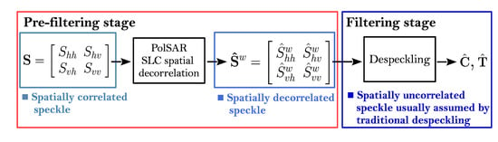
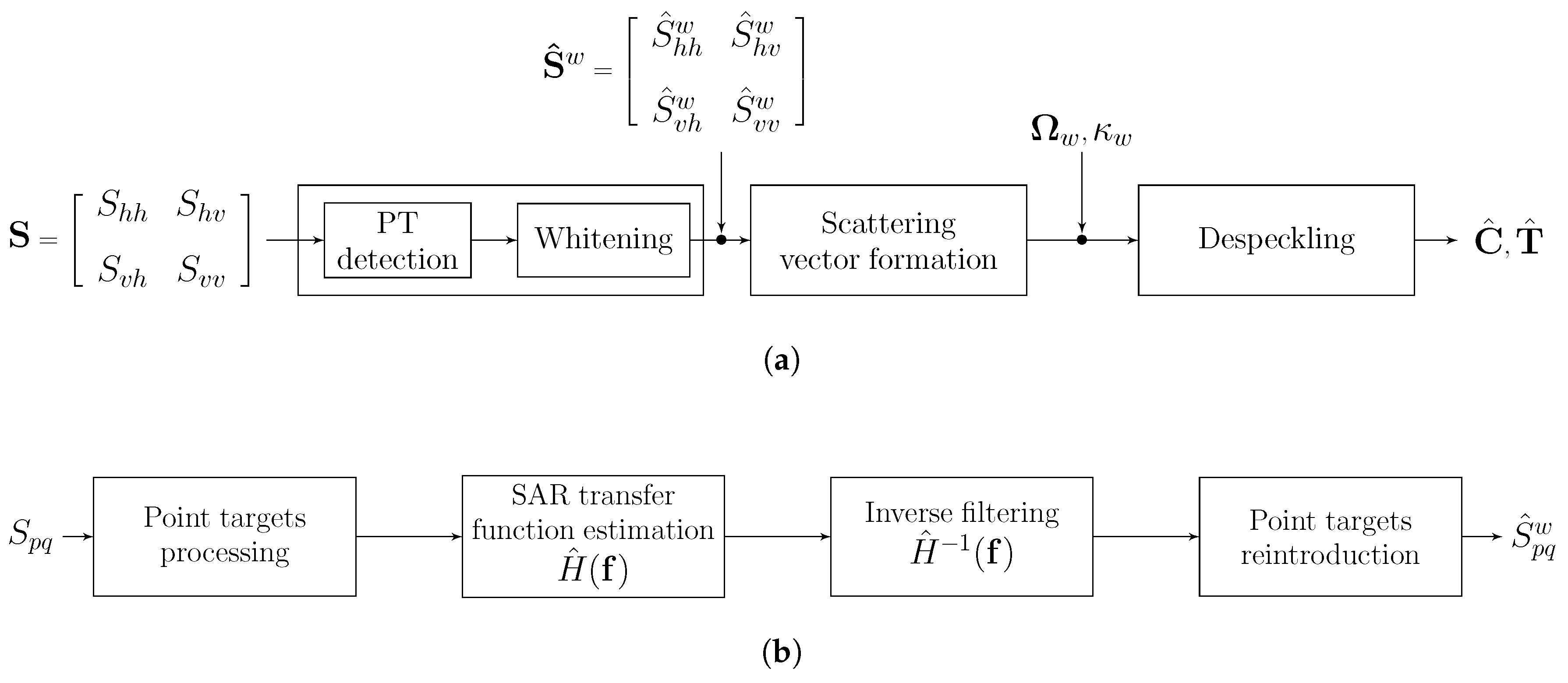
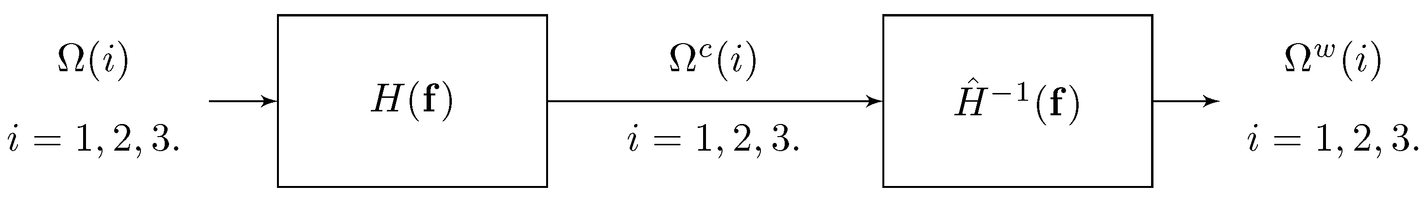
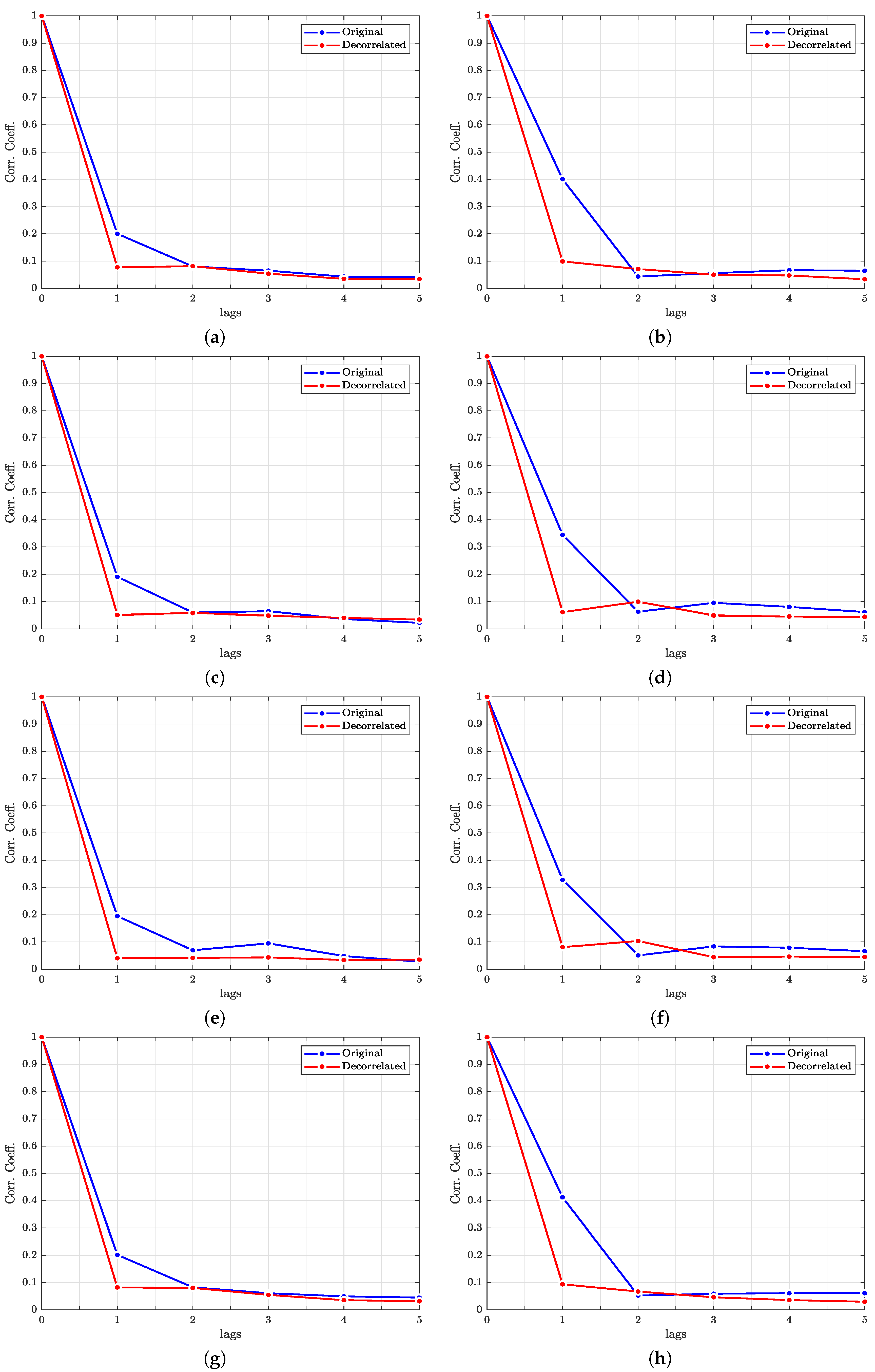
2.2. Spatial Decorrelation of Complex Speckle

Here, following the guidelines of [24] we make use of the spectral properties of SLC SAR imagery derived by [31] to describe the decorrelation procedure for single-polarization SLC images. The extension to the polarimetric case, from scalar to vector data, is straightforward, since the SAR processor separately focuses each channel [1]. The starting point is to assume the observed scene as a set of point scatterers. Let S p q w ( r ) be the discrete complex scattering coefficient, an arbitrary element of the scattering matrix (1), where r = ( r x , r y ) denotes the 2D spatial coordinates. Under the hypothesis of fully developed speckle, S p q w ( r ) is assumed to be a white, zero-mean, circular symmetric Gaussian process, with variance σ p q ( r ) , which is the radar backscatter information we want to recover. The 2D signal at the output of the SAR processor can be formulated as:
S p q ( r ) = S p q w ( r ) h ( r )
or equivalently in the Fourier domain as:
S p q ( r ) = F 1 F S p q w ( r ) · H ( f ) .
In (8) and (9), we have supposed that the entire SAR acquisition chain can be modeled as a cascade of linear shift-invariant filters, summarized by their cumulative point spread function (PSF), h ( r ) . The most widespread formulation of the fully-developed speckle model for the single-polarization case is given by:
| S p q ( r ) | 2 = σ p q ( r ) · u u ( r ) ,
in which u u ( r ) is the multiplicative speckle noise, modeled as a white process having a negative exponential pdf. Such a model is valid when the SAR system is characterized by an ideal PSF, δ ( r ) . A more general formulation of the problem is given by:
| S p q ( r ) | 2 σ p q ( r ) · u s ( r ) ,
where u s ( r ) is the multiplicative speckle noise, spatially correlated because of the non-ideal SAR system transfer function and independent of σ p q ( r ) . A rigorous despeckling model should be based on (11) instead of (10). The rationale for using speckle decorrelation is exactly to remove the effects of the SAR system transfer function, restoring S p q w ( r ) from S p q ( r ) . In other words, we are facing a blind deconvolution problem that may be simplified assuming the SAR system transfer function to be a band-limited lowpass filter with cutoff frequency f c :
H ( f ) 0 | f | > | f c | .
Unlike other image restoration methods, any statistical assumptions on σ p q ( r ) are avoided; it can be demonstrated that an estimator of S ^ p q w ( r ) is given by:
S ^ p q w ( r ) = 1 { F S p q ( r ) · [ H ^ ( f ) ] 1 } | f | | f c | 0 otherwise .
In this way, the problem of blind deconvolution has been transformed into the spectral estimation of the SAR transfer function, H ( f ) , required to design the inverse filter and recover the original whiteness of the data. The transfer function mainly depends on the focusing window (Hamming, Kaiser, etc.) but also on possible oversampling of the raw data. The estimation of the SAR transfer function is performed using a least-squares minimization approach in the spectral domain starting from the original SLC data. Details of the procedure may be found in the original publication [24].

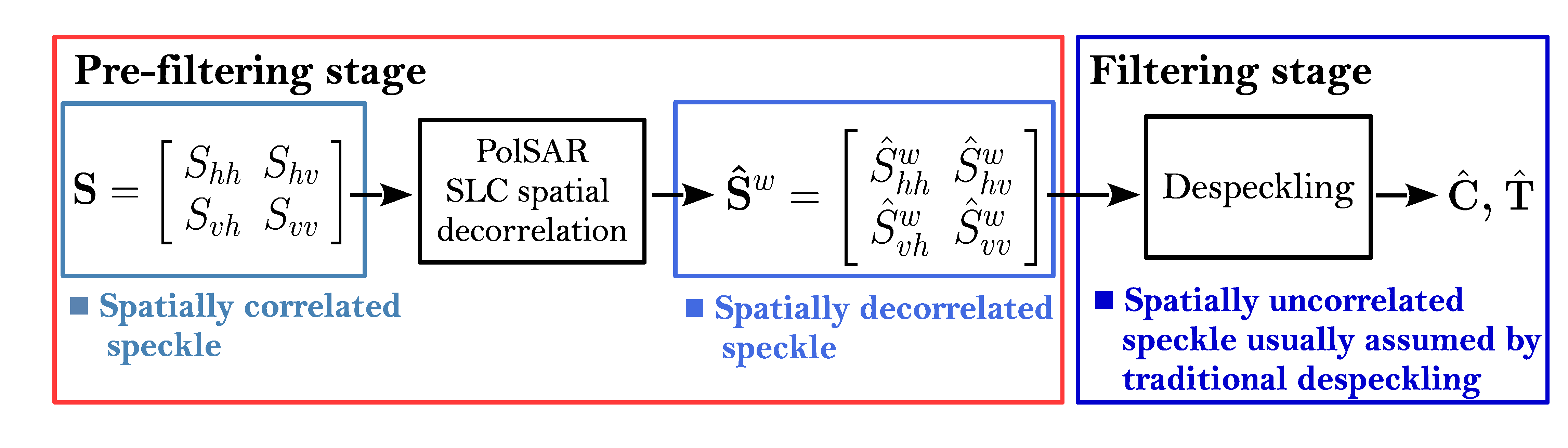
2.3. Processing of Point Targets

It is important to highlight that the effectiveness of the decorrelation procedure is diminished whenever the image statistics departs from the fully-developed speckle model; this occurs in the presence of point targets. For this reason, point targets must be removed and replaced with a synthetic speckle pattern, that is, a zero-mean white complex circular Gaussian pattern with variance proportional to the average energy of the neighboring pixels, before the Fourier-domain deconvolution process takes place.
For single-polarization SAR imagery, point targets can be detected by performing a percentile thresholding on the intensity or amplitude component [32] of the SLC image. In case of PolSAR data, the detection of point targets should take advantage of the capability of polarimetry to derive information about the nature of the scattering mechanisms involved in the backscattering process.
Point targets may be characterized by either strong-specular or double-bounce scattering [15]. The polarimetric information of these two scattering mechanisms are directly related to the terms T 11 = | S h h + S v v | 2 and T 22 = | S h h S v v | 2 of the coherency matrix (6). Hence, following the guidelines of [15], the detection of point targets can be performed by setting thresholds at the 98th percentiles of T 11 and T 22 ; namely, θ 11 98 and θ 22 98 . A binary map of candidate point targets, M C T , can be obtained as follows:
M C T ( r ) = 1 if T 11 ( r ) > θ 11 98 OR T 22 ( r ) > θ 22 98 0 otherwise .
To avoid the detection of isolated spikes instead of true point scatterers, a local screening with a 3 × 3 sliding window, W , is applied over the binary map of candidate point targets, M C T . A candidate pixel is detected as an actual point target and placed in the corresponding map M P T , if the number of its neighbors in the local window is greater than a predefined value, K:
M P T ( r ) = 1 if W M C T ( r ) > K 0 otherwise .
In other words, only clustered pixels with strong surface or double-bounce backscattering are suitable for being detected as point targets. In our implementation we set K = 5 , as recommended by Lee et al. [15]. According to their study, point targets are unique for all polarizations, and the empirical criterion to find them does not consider the crossed polarizations. Since point targets should be removed before the decorrelation and inserted back in the decorrelated data, in all channels separately, in principle it might happen that some pixels are detected as though they contains targets, while they actually contain more or less developed speckle in the cross-polar channels. The removal/reinsertion of targets and the separate decorrelation will leave small patches with correlated noise in the crossed channels.
It is worth mentioning that the proposed whitening scheme significantly relies on a proper point-target detection. As a matter of fact, the whitening operation removes the effects of the focusing window, meaning that over distributed targets the spatial correlation will be removed, whereas on strong hard-targets, if not correctly removed and replaced, there will be undesirable cross-like features, resembling the SAR PSF, for the increased sidelobes’ level. In other words, targets will be defocused, as if they had been originally processed without tapering window. This highlights the importance of the point-targets’ processing before the actual spectrum-flattening operation.
In this sense, the procedure of percentile thresholding followed by screening, used for its simplicity, could be replaced by some more refined point-targets detectors. For instance, a tailored procedure, decomposing single-polarization SAR imagery in speckle dominated areas and point targets, was proposed in [33]. The adaptation to PolSAR data of such a methodology, where a-contrario criterion with explicit control of the number of false detections is employed to detect subpixel positions of point targets, could be utilized for the present case, instead of [15].

2.4. Spatial Decorrelation of PolSAR SLC Data

Although the whitening procedure described in Section 2.2 holds for single-polarization SAR data, the extension to the polarimetric case is straightforward. Since the four polarimetric channels are processed independently of one another, as pointed out in [1], on page 343, the whitening procedure of PolSAR data, depicted by Figure 1, can be obtained by applying the decorrelation procedure to each polarimetric channel, separately. Equivalently, we apply the whitening stage to each element of the scattering matrix S , or the lexicographic scattering vector Ω , before any multilook or detection operation is performed. In this way, the spatial autocorrelation of the speckle in each polarimetric channel is removed without introducing crosstalk between polarizations. The spatial decorrelation procedure for polarimetric SAR data can be summarized as follows:
Spatial Decorrelation of Speckle for PolSAR Data
1. Detection of point targets by means of (14) and (15).
2. For each element of S :
    2.1. Replacement of point targets with a complex Gaussian speckle pattern.
    2.2. Estimation of SAR system transfer function H ^ ( f ) .
    2.3. Estimation of complex scattering coefficient S ^ p q w ( r ) by means of (13).
    2.4 Reintroduction of point targets in S ^ p q w ( r ) .

3. PolSAR Data Simulation

Speckle is an intrinsic and fundamental component of the SAR signal, which means that it is impossible to have access to a SAR signal measured without speckle. This fact prevents us from having a reference on which to compare the performance of different speckle filters. For this reason, we opted for simulated PolSAR data. A viable strategy for PolSAR data simulation has been proposed in [28] and is briefly recalled hereafter. The simulation of a PolSAR image mainly comprises two steps: the simulation of the image morphology, i.e., the spatial structure of the image, and the simulation of the polarimetric scattering classes, bearing the polarimetric information. The former is accomplished by generating a random spatial pattern, according to the number of scattering classes that are simulated, while the latter is obtained from a real PolSAR dataset.
For instance, using the NASA/JPL AIRSAR, L-band, and the 4-look dataset of the San Francisco Bay, the H A α ¯ polarimetric decomposition theorem [34] was performed, and for each partitioned region of the H α ¯ plane, the class centroid, expressed in terms of coherency T (or covariance C ) matrix, was selected to be the representative of the corresponding scattering class, which was associated to a specific location in the image structure. In this way, a ground-truth (GT), speckle-free image was obtained.
Once the GT was generated, we turned our attention to the simulation of the SLC scattering vector, Ω . To do so, a Monte-Carlo simulation was performed. Firstly, the speckle vector was generated as a multivariate complex random variable with zero mean and identity covariance matrix:
υ N C 0 , I .
Then, for each GT, the Cholesky factorization of the related covariance matrix was performed:
C 1 / 2 C 1 / 2 H = C Ω = C 1 / 2 υ ,
which led to a simulated SLC lexicographic scattering vector, Ω , affected by spatially uncorrelated speckle. In our implementation, we generated 60 simulated images comprising five different polarimetric scattering classes: 12 structure images, each with five different speckle realizations. In addition, only after the SLC scattering vector was formed, we introduced another class modeling point targets, to which no speckle was added.
Since the goal of this study was evaluating the impact of a spatial decorrelation of the noise on the performance of polarimetric speckle filters, the next step was the generation of an SLC scattering vector affected by spatially autocorrelated noise. To that end, each element of Ω was multiplied in the frequency domain by a separable 2D Hamming window, with unity power gain:
Ω c ( i ) = 1 Ω ( i ) · H ( f ) i = 1 : [ S h h ] , 2 : [ 2 S h v ] , 3 : [ S v v ] ,
where:
H ( f ) = α ( 1 α ) · cos 2 π f F F 2 f F 2 .
The 2D spatial frequency, f ( f x , f y ) , is upper-bounded in modulus by half of the sampling frequency F ( F x , F y ) .
The choice of α is crucial, since it determines the degree of spectral smoothness, that is, the amount of bandwidth that is filtered out, and consequently, the level of spatial correlation introduced in the data. Typical values employed by commercial SAR processors are 0 . 6 α 0 . 7 , introducing a statistical correlation of intensity at lag one, approximately between 0.3 and 0.2. In our simulations, we decided to use the higher value, α = 0 . 7 , thereby introducing a spatial correlation at lag one not greater than 20%. In other words, we decided to evaluate the effects of speckle decorrelation in the case of a low-medium value of spatial correlation. It is important to remark that whenever a higher level of correlation is present in the data, the trends found in this work may be even more pronounced.
Finally, in order to obtain a decorrelated SLC scattering vector, we applied the decorrelation method of Section 2.4, to yield:
Ω w ( i ) = 1 Ω c ( i ) · [ H ^ 1 ( f ) ] i = 1 , 2 , 3 .
That way, we had made available three cases on which to compare the behavior of the polarimetric speckle filters: uncorrelated, correlated, and whitened (spatially decorrelated) correlated SLC images. Figure 2 summarizes the procedure for simulating spatially correlated and decorrelated SLC data. Figure 3 and Figure 4 show an example of a simulated image and the corresponding power spectra of the VV channel for the three aforementioned cases, respectively. ρ A C F denotes the correlation coefficient (CC) computed on the single-look intensity VV component. It is noteworthy that the decorrelation stage effectively recovers a correlation level similar to that of the uncorrelated case.

4. Simulations and Results

4.1. Experimental Setup

In this study, the following polarimetric speckle filters were considered: the traditional boxcar filter, the refined Lee filter [35], the model-based (MB) PolSAR filter [36], the scattering model-based (SMB) speckle filter [37], and the intensity-driven adaptive-neighborhood (IDAN) filter [38]. In the simulations, each filter was implemented using the SAR Data Processing Educational ToolBox, PolSARPRO version 5.0 [39]. It is important to highlight that we were not interested in comparing or ranking different speckle filters, but only in evaluating the effects of a spatial decorrelation of speckle on their performance.
The following polarimetric features have been evaluated:
Intensities: they are the diagonal element of the covariance matrix (5):
σ p q = | S p q | 2 .
If multiplied by 4 π , they provide the so-called radar cross section, usually expressed in dB.
SPAN, also known as total power: it is the sum of the polarimetric intensities and is given by the trace of (5):
SPAN = | S h h | 2 + 2 | S h v | 2 + | S v v | 2 .
Coherences: the polarimetric coherences, or degrees of coherence, are given by the moduli of the normalized versions of the complex polarimetric correlations (off-diagonal terms of (5)):
ρ m n p q = S m n S p q * S m n 2 S p q 2 .
These quantities provide a correlation measure between the polarimetric responses, strongly related to orientation (geometric factors) or dielectric properties (biophysical factors) of the local scattering elements within the SAR resolution cell.
Eigenvalues: these parameters are obtained from the eigen-decomposition of the coherency matrix (6):
T = U Σ U 1
where Σ is the 3 × 3 diagonal matrix with non-negative real elements, i.e., the eigenvalues; and U = [ u 1 , u 2 , u 3 ] is the 3 × 3 unitary matrix composed by the three orthogonal eigenvectors, u 1 , u 2 , and u 3 [29]. As proposed in [40], T may be expanded into the sum of three independent terms, each related to a deterministic scattering mechanism, where the eigenvector u i specifies the type of scattering mechanism while the eigenvalue λ i denotes its relative magnitude:
T = i = 1 3 λ i u i u i H .
From the eigenvalues, several parameters have been derived over the last few decades. The H A α ¯ polarimetric decomposition theorem [34] is definitely one of the most renowned in the field of SAR polarimetry. Other examples of eigenvalue-based parameters are the polarization fraction (PF), the polarization anisotropy (PA) [41], and the radar vegetation index (RVI) [42].
Equivalent number of looks: the equivalent number of looks (ENL) parameter is an indicator of the speckle reduction capability of a filter. Over a homogeneous area, the higher the ENL, the better the speckle reduction. Its definition is given by:
ENL = μ ^ 2 σ ^ 2 ,
where μ ^ and σ ^ are the local mean and standard deviation, respectively, calculated with a sliding window over a polarimetric intensity channel. For simplicity, we have opted for the scalar ENL estimator based on the local coefficient of variation and computed for each diagonal element of C , separately. Alternatively, one might use the estimator proposed in [43], tailored to PolSAR data, where a unique ENL value is obtained taking into account all the elements of the covariance matrix, C .
The despeckling performances of the filters were evaluated in terms of normalized root mean square error (NRMSE):
Δ ( x ; x n s i m , n c l a s s ) f i l t e r = 1 N M i = 1 N j = 1 M x i , j x ^ i , j max ( x i , j ) 2 ,
in which N × M is the number of image pixels; and, for a given filter, x and x ^ are the GT and the estimated values of a particular feature, for the simulated image n s i m , and for pixels belonging to the scattering class n c l a s s . The sole feature that is not normalized in (27) is the polarimetric coherence, already normalized by definition.
That way, for each filter and for the set of considered features, we got an estimated error for every simulated image and for each scattering class. For each feature, errors were averaged over the scattering classes and over all the simulated images. Finally, in order to have a unique global value for each parameter, another average was applied along the polarimetric direction, with the exception of the SPAN, for which a unique value was already available. ENL (26) was averaged over the polarimetric intensity channels only.

4.2. Tests on Simulated PolSAR Data

In this section, we first describe the results obtained with simulated data. In order to have a more general assessment of the effects of spatial correlation on despeckling filters, we performed two types of simulations. One involved only spatial multilooking, i.e., a boxcar filter, with a variable number of looks, i.e., number of pixels averaged in the local window. Another includes also all the other despeckling filters mentioned in Section 4.1.
The plots of Figure 5 show the NRMSE as a function of number of looks for each polarimetric feature. From first glance a general trend is noticeable: the estimation error relative to the case of correlated speckle is always the highest, while for the uncorrelated case is always the lowest. Interestingly, the spatial decorrelation produces an error very similar to that of the uncorrelated case. Another general trend is that the estimation error tends to vanish as the number of looks increases. This may suggest that large windows better cope with correlated noise, since the correlation length of speckle is much lower than the length of the filter, and thus unable to severely bias the local average, that is, the output of the box filter.
Not surprisingly, the most evident benefit of the speckle decorrelation is for ENL. Figure 6 reports the estimated ENL: the uncorrelated case shows the higher values, as expected from theory, the looks being statistically independent. The correlated case, on the other hand, shows the lowest values. The decorrelated case attains an ENL similar to that of the uncorrelated case, without reaching its values, because of the slight loss of bandwidth, caused by the focusing window, which may no longer be recovered by the decorrelation process, and thus introduces a slight oversampling.
The spider plots in Figure 7 show the despeckling performances of all the other filters that have been investigated, besides the boxcar one. The results highlight that statistical filters more developed than the plain boxcar filter benefit from the spatial decorrelation of the fully-developed speckle. There is a unique exception for intensity, as estimated by the 7×7 refined Lee filter, for which the case of correlated noise is better than the decorrelated case. While all local spatial filters substantially share this behavior, nonlocal filters, e.g., [8,9,14], are expected to be more or less sensitive to correlation, depending on the landscape, because they may average samples that are more or less sparse within the search area surrounding the current pixel.

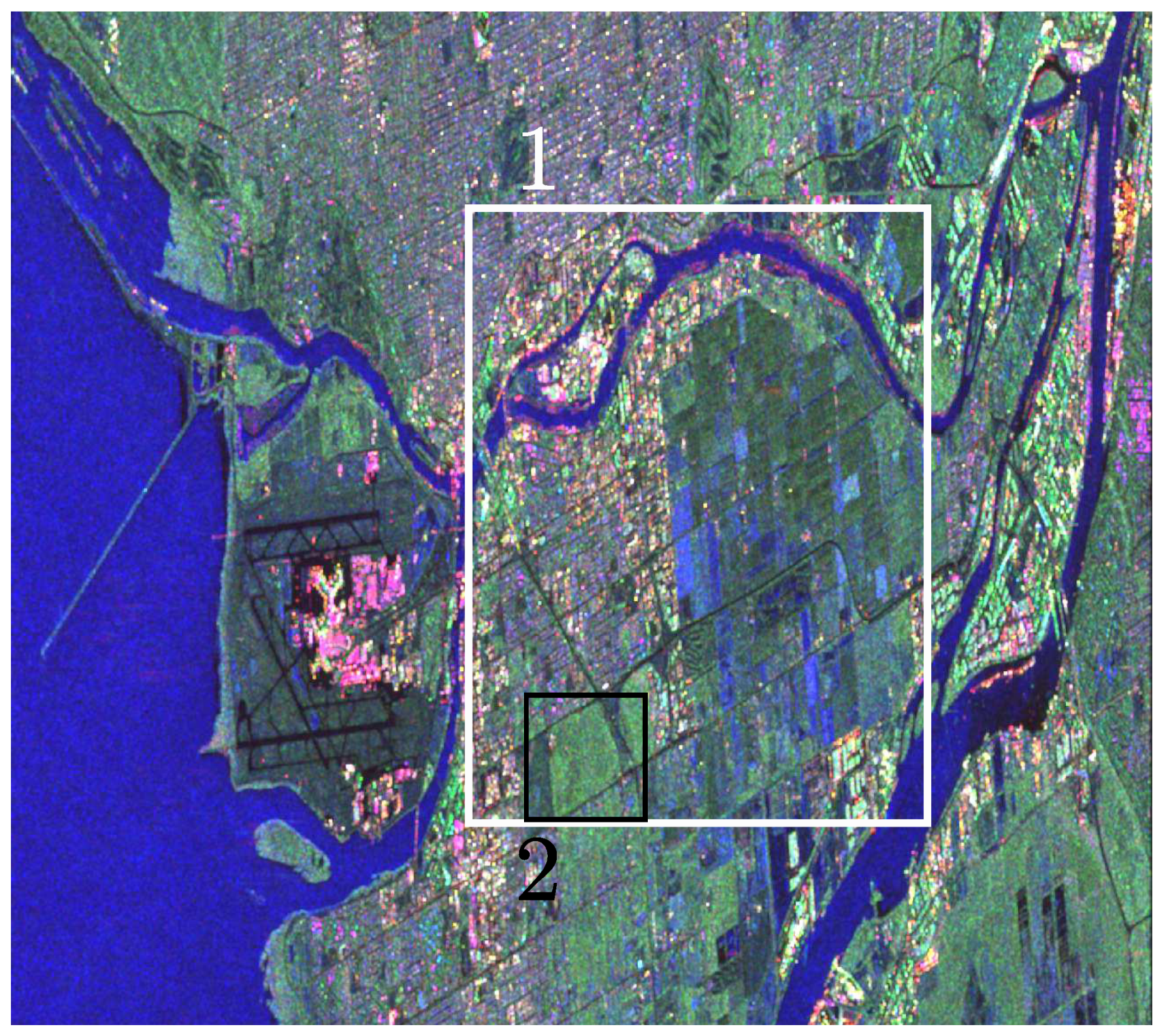
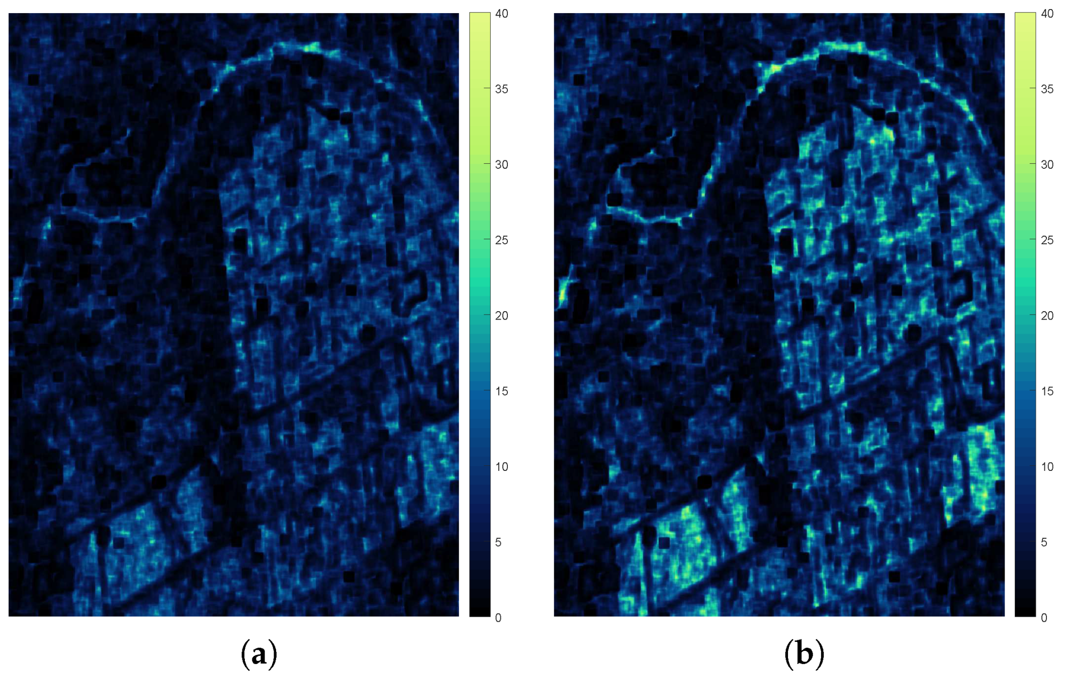
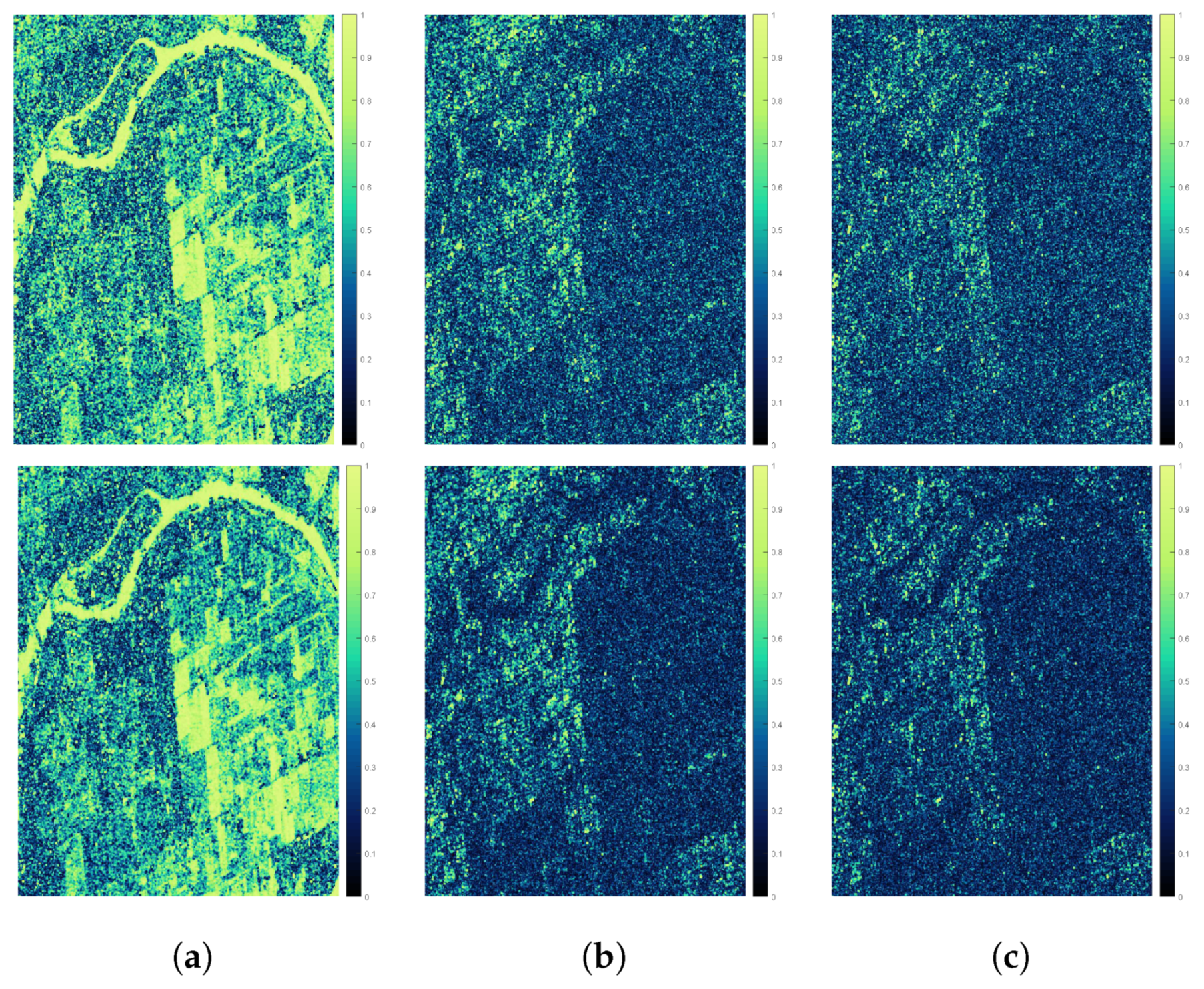
4.3. Tests on True PolSAR Data

Eventually, we applied the proposed speckle decorrelation procedure to a real Radarsat-2 fully-polarimetric dataset. The test image is a Fine Quad-Pol SLC of the Vancouver sample dataset. Figure 8 shows the Pauli RGB composite, 25-looks, of the region. Two study areas have been selected. The first area, namely, Subset 1, including a very heterogeneous scenario, with urban, textured and homogeneous areas, provides an appropriate contest for testing the validity of the proposed methodology, without relying on specific ground reflectivity assumptions. The other area, namely, Subset 2, comprises a spatial region highly dominated by volume scattering.
Before applying any despeckling operation, we selected a small patch characterized by strong homogeneity, in order to assess the speckle autocorrelation function (ACF) of the original and whitened SLC images. Figure 9 shows the speckle ACF of each polarimetric channel for the two cases under concern. Three main aspects are directly noticeable. First, the speckle correlation of the original SLC is mainly confined to the first neighboring pixel and can be neglected starting from the lag two onward. This observation gives an idea of the speckle correlation length induced by the broadening of the SAR impulse response mainly caused by the windowing operation.
The second aspect involves the different amounts of correlation in range and in azimuth. This effect is related to the different pre-filters that the SAR signal encounters in the image formation process. The azimuth pre-filter comprises the azimuth antenna pattern (AAP) weighting and the Doppler modulation. The former, given its resulting frequency selectivity, is a spatial correlation source. On the other hand, the range pre-filter representing the envelope of the full-bandwidth chirp signal, does not introduce significant correlation. The use of tapering windows in the SAR processor reinforces the frequency selectivity of the AAP and reduces the useful chirp bandwidth, simultaneously causing the reduction of sidelobes, the resolution loss, and the introduction of spatial correlation.
The third noteworthy aspect is how the decorrelation stage leads to a negligible spatial correlation on the eight neighboring pixels, in all polarimetric channels. In other words, after the decorrelation operation the noise can be considered white, or more exactly, spatially uncorrelated. If we apply a boxcar filter of size L, performing a multi-looking with L nominal looks on the whitened image, we will find that the measured ENL is higher and more closely attains its limit value, L. Figure 10 shows the ENL averaged over the three polarizations for the case of correlated and decorrelated speckles. It is possible to note how the ENL significantly increases over homogeneous areas, especially over crops and rivers, thereby suggesting a better speckle reduction capability of despeckling filter, whenever the complex image has been spatially decorrelated. Figure 11 reports the three polarimetric coherences computed over Subset 1. The sharper and slightly darker appearance of the three polarimetric coherences stands out for the decorrelated case. The coherence bias reduction was already observed when the whitening procedure was applied before InSAR processing [25].
A possible explanation of the bias reduction is the following. The maximum likelihood (ML) estimate of the sample coherence is well-known to be biased toward higher values, especially between areas of differing low coherence [26]. Such a bias decreases as the number of independent samples employed for its estimation increases. In the case of correlated samples, the bias is greater, due to the statistical dependence among samples introduced by correlation. The decorrelation operation increases the number of independent samples involved in the estimation; thus, it leads to a reduction in the bias.
Figure 12 shows all the other radiometric quantities, computed over the vegetated region of Subset 2. The volume scattering mechanism is clearly visible in the cross-polar intensity, which is sensitive to any depolarization effect. In all the features, the improvement in the estimation, even though subtle, can be noticed as a less granular appearance, visually confirming a better despeckling ability, and slightly darker colors, witnessing a less biased estimation.
Ultimately, tests on true data from Radarsat-2 have the sole objective of showing, through proper lookup display, that the point measurements are in agreement with the objective trends achieved on the simulated data and that the capability of filters to preserve edges and textures is better if the noise is uncorrelated.

5. Conclusions

Originally proposed for the despecking of single-look detected SAR images, the idea of reducing the spatial correlations of the fully-developed complex noise, caused by the range and azimuth focusing windows in the Fourier domain, used by the SAR processor to avoid Gibbs effects on strong scatterers and point targets, seems rewarding for information extraction from PolSAR data as well. Thanks to the use of a PolSAR simulator, and hence to the availability of a GT, it was shown that polarimetric despeckling and features estimation (intensity, SPAN, eigenvalue, and coherence) are more accurate. Specifically, the noise correlation causes underestimation of local variances, and hence overestimation of coherences, because the sample domain is not locally ergodic. The decrement in polarimetric features-estimation accuracy induced by correlation is moderate, yet non-negligible, and might diminish the performance attainable by analysis methods using geo/biophysical modeling based on estimation of polarimetric features. Although there are many simple and effective despeckling methods available at present, it is not doubted that a great number of them, including those contained in the PolSARPro software toolbox, were devised under the assumption of spatially uncorrelated noise. Future developments will concern the use of spatially-decorrelated SLC images for SAR tomography [44], in which coherent processing makes use of the phase history. As a final consideration, the proposed procedure, that is, decorrelation followed by despeckling and/or features extimation, has no disadvantages other than computational.

Author Contributions

Conceptualization, F.A and L.A.; methodology, F.A.; software, A.A.; validation, M.G. and L.A.; writing—original draft preparation, A.A. and F.A.; writing—review and editing, M.G. and L.A.; supervision, M.G. All authors have read and agreed to the published version of the manuscript.

Funding

This research received no external funding.

Acknowledgments

The authors are grateful to MDA Geospatial Services Inc. for providing the Radarsat-2 Vancouver sample dataset. Radarsat-2 Data and Products © MDA Geospatial Services Inc. (2008) All Rights Reserved. Radarsat is an official mark of the Canadian Space Agency.

Conflicts of Interest

The authors declare no conflict of interest.

References

  1. Cloude, S. Polarisation: Applications in Remote Sensing; Oxford University Press: Oxford, UK, 2009. [Google Scholar]
  2. Argenti, F.; Lapini, A.; Alparone, L.; Bianchi, T. A tutorial on speckle reduction in synthetic aperture radar images. IEEE Geosci. Remote Sens. Mag. 2013, 1, 6–35. [Google Scholar] [CrossRef] [Green Version]
  3. Touzi, R. A review of speckle filtering in the context of estimation theory. IEEE Trans. Geosci. Remote Sens. 2002, 40, 2392–2404. [Google Scholar] [CrossRef]
  4. Achim, A.; Tsakalides, P.; Bezerianos, A. SAR image filtering based on the heavy-tailed Rayleigh model. IEEE Trans. Image Process. 2006, 15, 2686–2693. [Google Scholar] [CrossRef] [PubMed] [Green Version]
  5. Achim, A.; Tsakalides, P.; Bezerianos, A. SAR image denoising via Bayesian wavelet shrinkage based on heavy-tailed modeling. IEEE Trans. Geosci. Remote Sens. 2003, 41, 1773–1784. [Google Scholar] [CrossRef]
  6. Argenti, F.; Rovai, N.; Alparone, L. Despeckling SAR images in the undecimated wavelet domain: A MAP approach. In Proceedings of the IEEE International Conference on Acoustics, Speech, and Signal Processing, Philadelphia, PA, USA, 23 March 2005; Volume IV, pp. 541–544. [Google Scholar]
  7. Argenti, F.; Torricelli, G.; Alparone, L. MMSE filtering of generalised signal-dependent noise in spatial and shift-invariant wavelet domains. Signal Process. 2006, 86, 2056–2066. [Google Scholar] [CrossRef]
  8. Deledalle, C.A.; Denis, L.; Tupin, F.; Reigber, A.; Jager, M. NL-SAR: A unified nonlocal framework for resolution-preserving (Pol)(In)SAR denoising. IEEE Trans. Geosci. Remote Sens. 2015, 53, 2021–2038. [Google Scholar] [CrossRef] [Green Version]
  9. Vitale, S.; Cozzolino, D.; Scarpa, G.; Verdoliva, L.; Poggi, G. Guided patchwise nonlocal SAR despeckling. IEEE Trans. Geosci. Remote Sens. 2019, 57, 6484–6498. [Google Scholar] [CrossRef] [Green Version]
  10. Lattari, F.; Gonzalez Leon, B.; Asaro, F.; Rucci, A.; Prati, C.; Matteucci, M. Deep learning for SAR image despeckling. Remote Sens. 2019, 11, 1532. [Google Scholar] [CrossRef] [Green Version]
  11. Novak, L.M.; Burl, M.C. Optimal speckle reduction in polarimetric SAR imagery. IEEE Trans. Aerosp. Electron. Syst. 1990, 26, 293–305. [Google Scholar] [CrossRef]
  12. Touzi, R.; Lopès, A. The principle of speckle filtering in polarimetric SAR imagery. IEEE Trans. Geosci. Remote Sens. 1994, 32, 1110–1114. [Google Scholar] [CrossRef]
  13. López-Martínez, C.; Fabregas, X. Polarimetric SAR speckle noise model. IEEE Trans. Geosci. Remote Sens. 2003, 41, 2232–2242. [Google Scholar] [CrossRef] [Green Version]
  14. Torres, L.; Sant’Anna, S.J.S.; Da Costa Freitas, C.; Frery, A.C. Speckle reduction in polarimetric SAR imagery with stochastic distances and nonlocal means. Pattern Recognit. 2014, 47, 141–157. [Google Scholar] [CrossRef] [Green Version]
  15. Lee, J.S.; Ainsworth, T.L.; Wang, Y.; Chen, K. Polarimetric SAR speckle filtering and the extended sigma filter. IEEE Trans. Geosci. Remote Sens. 2015, 53, 1150–1160. [Google Scholar] [CrossRef]
  16. Gao, G. Statistical modeling of SAR images: A survey. Sensors 2010, 10, 775–795. [Google Scholar] [CrossRef]
  17. Aiazzi, B.; Alparone, L.; Baronti, S. Information-theoretic heterogeneity measurement for SAR imagery. IEEE Trans. Geosci. Remote Sens. 2005, 43, 619–624. [Google Scholar] [CrossRef]
  18. D’Elia, C.; Ruscino, S.; Abbate, M.; Aiazzi, B.; Baronti, S.; Alparone, L. SAR image classification through information-theoretic textural features, MRF segmentation, and object-oriented learning vector quantization. IEEE J. Sel. Top. Appl. Earth Obs. Remote Sens. 2014, 7, 1116–1126. [Google Scholar] [CrossRef]
  19. Garzelli, A. Wavelet-based fusion of optical and SAR image data over urban area. In International Archives of the Photogrammetry Remote Sensing and Spatial Information Sciences—ISPRS Archives, Proceedings 2002 International Symposium of ISPRS Commission III on Photogrammetric Computer Vision, PCV 2002, Graz; Austria, 9–13 September 2002; International Society for Photogrammetry and Remote Sensing: Hanover, Germany, 2002; Volume 34, pp. 1–4. [Google Scholar]
  20. Alparone, L.; Facheris, L.; Baronti, S.; Garzelli, A.; Nencini, F. Fusion of multispectral and SAR images by intensity modulation. In Proceedings of the 7th International Conference on Information Fusion, FUSION 2004, Stockholm, Sweden, 28 June–1 July 2004; Volume 2, pp. 637–643. [Google Scholar]
  21. Aiazzi, B.; Alparone, L.; Baronti, S.; Garzelli, A.; Zoppetti, C. Nonparametric change detection in multitemporal SAR images based on mean-shift clustering. IEEE Trans. Geosci. Remote Sens. 2013, 51, 2022–2031. [Google Scholar] [CrossRef]
  22. Nascimento, A.D.C.; Frery, A.C.; Cintra, R.J. Detecting changes in fully polarimetric SAR imagery with statistical information theory. IEEE Trans. Geosci. Remote Sens. 2019, 57, 1380–1392. [Google Scholar] [CrossRef] [Green Version]
  23. Oliver, C.; Quegan, S. Understanding Synthetic Aperture Radar Images; The SciTech Radar and Defense Series; SciTech Publishing Inc.: Raleigh, NC, USA, 2004. [Google Scholar]
  24. Lapini, A.; Bianchi, T.; Argenti, F.; Alparone, L. Blind speckle decorrelation for SAR image despeckling. IEEE Trans. Geosci. Remote Sens. 2014, 52, 1044–1058. [Google Scholar] [CrossRef] [Green Version]
  25. Sica, F.; Alparone, L.; Argenti, F.; Fornaro, G.; Lapini, A.; Reale, D. Benefits of blind speckle decorrelation for InSAR processing. In Proceedings of the SAR Image Analysis, Modeling, and Techniques XIV, Amsterdam, The Netherlands, 24–25 September 2014; Proceedings of SPIE-The International Society for Optical Engineering: Bellingham, WA, USA, 2014; Volume 9243. [Google Scholar]
  26. Touzi, R.; Lopès, A.; Bruniquel, J.; Vachon, P.W. Coherence estimation for SAR imagery. IEEE Trans. Geosci. Remote Sens. 1999, 37, 135–149. [Google Scholar] [CrossRef] [Green Version]
  27. Aiazzi, B.; Alparone, L.; Baronti, S.; Garzelli, A. Coherence estimation from multilook incoherent SAR imagery. IEEE Trans. Geosci. Remote Sens. 2003, 41, 2531–2539. [Google Scholar] [CrossRef]
  28. Foucher, S.; López-Martínez, C. Analysis, evaluation, and comparison of polarimetric SAR speckle filtering techniques. IEEE Trans. Image Process. 2014, 23, 1751–1764. [Google Scholar] [CrossRef] [PubMed]
  29. Lee, J.S.; Pottier, E. Polarimetric Radar Imaging: From Basics to Applications; Optical Science and Engineering; CRC Press: Boca Raton, FL, USA, 2009. [Google Scholar]
  30. Yueh, S.H.; Kong, J.A.; Jao, J.K.; Shin, R.T.; Novak, L.M. K-distribution and polarimetric terrain radar clutter. J. Electromagn. Waves Appl. 1989, 3, 747–768. [Google Scholar] [CrossRef]
  31. Madsen, S.N. Spectral properties of homogeneous and nonhomogeneous radar images. IEEE Trans. Aerosp. Electron. Syst. 1987, AES-23, 583–588. [Google Scholar] [CrossRef] [Green Version]
  32. Bianchi, T.; Argenti, F.; Lapini, A.; Alparone, L. Amplitude vs intensity Bayesian despeckling in the wavelet domain for SAR images. Digit. Signal Process. 2013, 23, 1353–1362. [Google Scholar] [CrossRef] [Green Version]
  33. Abergel, R.; Denis, L.; Ladjal, S.; Tupin, F. Subpixellic methods for sidelobes suppression and strong targets extraction in single look complex SAR images. IEEE J. Sel. Top. Appl. Earth Obs. Remote Sens. 2018, 11, 759–776. [Google Scholar] [CrossRef] [Green Version]
  34. Cloude, S.R.; Pottier, E. An entropy based classification scheme for land applications of polarimetric SAR. IEEE Trans. Geosci. Remote Sens. 1997, 35, 68–78. [Google Scholar] [CrossRef]
  35. Lee, J.S.; Grunes, M.R.; De Grandi, G. Polarimetric SAR speckle filtering and its implication for classification. IEEE Trans. Geosci. Remote Sens. 1999, 37, 2363–2373. [Google Scholar]
  36. López-Martínez, C.; Fabregas, X. Model-based polarimetric SAR speckle filter. IEEE Trans. Geosci. Remote Sens. 2008, 46, 3894–3907. [Google Scholar] [CrossRef]
  37. Lee, J.S.; Grunes, M.R.; Schuler, D.L.; Pottier, E.; Ferro-Famil, L. Scattering-model-based speckle filtering of polarimetric SAR data. IEEE Trans. Geosci. Remote Sens. 2006, 44, 176–187. [Google Scholar]
  38. Vasile, G.; Trouve, E.; Lee, J.S.; Buzuloiu, V. Intensity-driven adaptive-neighborhood technique for polarimetric and interferometric SAR parameters estimation. IEEE Trans. Geosci. Remote Sens. 2006, 44, 1609–1621. [Google Scholar] [CrossRef] [Green Version]
  39. Pottier, E.; Ferro-Famil, L. PolSARPro V5.0: An ESA educational toolbox used for self-education in the field of POLSAR and POL-INSAR data analysis. In Proceedings of the 2012 IEEE International Geoscience and Remote Sensing Symposium, Munich, Germany, 22–27 July 2012; pp. 7377–7380. [Google Scholar]
  40. Cloude, S.R.; Pottier, E. A review of target decomposition theorems in radar polarimetry. IEEE Trans. Geosci. Remote Sens. 1996, 34, 498–518. [Google Scholar] [CrossRef]
  41. Ainsworth, T.L.; Cloude, S.R.; Lee, J.S. Eigenvector analysis of polarimetric SAR data. In Proceedings of the IEEE International Geoscience and Remote Sensing Symposium, Toronto, ON, Canada, 24–28 June 2002; pp. 626–628. [Google Scholar]
  42. Van Zyl, J.J. Application of Cloude’s target decomposition theorem to polarimetric imaging radar data. In Radar Polarimetry 1992; Proceedings of SPIE-The International Society for Optical Engineering: Bellingham, WA, USA, 1993; Volume 1748, pp. 184–191. [Google Scholar]
  43. Anfinsen, S.N.; Doulgeris, A.P.; Eltoft, T. Estimation of the equivalent number of looks in polarimetric synthetic aperture radar imagery. IEEE Trans. Geosci. Remote Sens. 2009, 47, 3795–3809. [Google Scholar] [CrossRef]
  44. Lombardini, F.; Cai, F. Generalized-Capon method for Diff-Tomo SAR analyses of decorrelating scatterers. Remote Sens. 2019, 11, 412. [Google Scholar] [CrossRef] [Green Version]
Figure 1. PolSAR spatial decorrelation processing and despeckling. (a): whole processing chain; (b): close-up of whitening box.
Remotesensing 12 00331 g001
Figure 2. Simulation of correlated and decorrelated lexicographic single-look complex (SLC) scattering vectors.
Remotesensing 12 00331 g002
Figure 3. Example of a 256×256 simulated PolSAR image in Pauli RGB (red: | S h h S v v | 2 , green: 2 | S h v | 2 , blue: | S h h + S v v | 2 ). (a) Multilook complex (MLC) ground-truth (GT); (b) SLC with uncorrelated speckle; (c) SLC with correlated speckle; (d) SLC with spatially-decorrelated correlated speckle.
Remotesensing 12 00331 g003
Figure 4. Normalized power spectra of simulated SLC (VV channel). (a) Uncorrelated speckle, ρ A C F = 0 . 0020 ; (b) correlated speckle, ρ A C F = 0 . 1886 ; (c) decorrelated speckle, ρ A C F = 0 . 0110 .
Remotesensing 12 00331 g004
Figure 5. Normalized root mean square error (NRMSE) versus number of looks (size of box filter) for (a) intensity; (b) SPAN; (c) eigenvalue; (d) coherence.
Remotesensing 12 00331 g005
Figure 6. Estimated equivalent number of looks (ENL) as a function of increasing local window size.
Remotesensing 12 00331 g006
Figure 7. Spider plots of the despeckling performances for uncorrelated (green), correlated (yellow), and decorrelated (red) speckles: (a) boxcar 3 × 3 , (b) boxcar 5 × 5 , (c) boxcar 7 × 7 , (d) refined Lee 5 × 5 , (e) refined Lee 7 × 7 , (f) Lopes 5 × 5 , (g) Lopes 7 × 7 , (h) scattering model-based (SMB), (i) intensity-driven adaptive-neighborhood (IDAN).
Remotesensing 12 00331 g007
Figure 8. Pauli RGB, 25-look, of a portion of the Radarsat-2 Vancouver sample dataset, highlighting two specific subsets, (1 and 2), analyzed in the investigation.
Remotesensing 12 00331 g008
Figure 9. Speckle autocorrelation function computed over a homogeneous patch along the range direction (left column) and the azimuth direction (right column) of the original and decorrelated single-look intensity. (a,b) HH; (c,d) HV; (e,f) VH; (g,h) VV.
Remotesensing 12 00331 g009
Figure 10. Estimated ENL by means of an 11 × 11 sliding window: (a) original; (b) decorrelated.
Remotesensing 12 00331 g010
Figure 11. Polarimetric coherences for Subset 1 of Figure 8. (Top): Boxcar 5 × 5 without preliminary decorrelation stage. (Bottom): Boxcar 5 × 5 with prior spatial decorelation stage. (a) HHVV coherence; (b) HHHV coherence; (c) VVHV coherence.
Remotesensing 12 00331 g011
Figure 12. Boxcar 5 × 5 filtered polarimetric parameters for Subset 2 of Figure 8. (+,+): original data, decorrelated data. (a,b): SPAN; (c,d): σ h h ; (e,f): σ h v ; (g,h): σ v h ; (i,j): σ v v ; (k,l): λ 1 ; (m,n): λ 2 ; (o,p): λ 3 . All features are shown in logarithmic scale (dB).
Remotesensing 12 00331 g012

