Evaluation of E Layer Dominated Ionosphere Events Using COSMIC/FORMOSAT-3 and CHAMP Ionospheric Radio Occultation Data

Abstract

At certain geographic locations, especially in the polar regions, the ionization of the ionospheric E layer can dominate over that of the F2 layer. The associated electron density profiles show their ionization maximum at E layer heights between 80 and 150 km above the Earth’s surface. This phenomenon is called the “E layer dominated ionosphere” (ELDI). In this paper we systematically investigate the characteristics of ELDI occurrences at high latitudes, focusing on their spatial and temporal variations. In our study, we use ionospheric GPS radio occultation data obtained from the COSMIC/FORMOSAT-3 (Constellation Observing System for Meteorology, Ionosphere, and Climate/Formosa Satellite Mission 3) and CHAMP (Challenging Minisatellite Payload) satellite missions. The entire dataset comprises the long period from 2001 to 2018, covering the previous and present solar cycles. This allows us to study the variation of the ELDI in different ways. In addition to the geospatial distribution, we also examine the temporal variation of ELDI events, focusing on the diurnal, the seasonal, and the solar cycle dependent variation. Furthermore, we investigate the spatiotemporal dependency of the ELDI on geomagnetic storms.

1. Introduction

Ionospheric radio occultation (IRO) is a space-based observation technique for studying the Earth’s ionosphere on a global scale. It is based on the measurement of phase changes of global navigation satellite system (GNSS) radio signals which are received onboard low Earth orbit (LEO) satellites. As the GNSS and LEO satellites orbit the Earth, the ionosphere is scanned by the radio links between them in the limb sounding mode. The measured phase changes partly depend on the ionosphere’s refractivity, which primarily depends on the electron density. In order to derive vertical electron density profiles from the bottom of the ionosphere up to the LEO satellite’s orbit height, the phase changes are inverted, for example by using the Abel inversion [1,2,3]. Compared to ground-based methods, IRO can be used to carry out global measurements, including atmospheric regions that are otherwise difficult to access, e.g., above the oceans. In contrast to ionosondes, IRO allows an investigation of both the bottomside and the topside ionosphere, if the LEO satellite’s orbit height is above the F2 layer height.

The analysis of IRO data, obtained onboard the CHAMP (Challenging Minisatellite Payload) and COSMIC/FORMOSAT-3 (Constellation Observing System for Meteorology, Ionosphere, and Climate/Formosa Satellite Mission 3) satellites for high latitudes of the northern hemisphere has shown numerous vertical electron density profiles characterized by the peak electron density of the E layer exceeding that of the F2 layer (NmE > NmF2). This anomaly has been called “E layer dominated ionosphere” (ELDI) by Mayer and Jakowski [4] and has been found to be located in the auroral zone. In contrast to sporadic E [5], which occupies only a very thin altitude range around 100 km primarily in mid-latitudes, ELDI is a high-latitude phenomenon in which a broader altitude range of the E layer shows a higher ionization than the F2 layer. The CHAMP data investigated by Mayer and Jakowski [4] covered two winter seasons at a high solar activity (2001/2002 and 2002/2003) and two at a relatively low solar activity (2005/2006 and 2006/2007), whereas the COSMIC data covered the winter season 2006/2007 in that study. An investigation of the CHAMP and COSMIC data has shown that the number of ELDI occurrences increased during local nighttime. Further analysis of the CHAMP data revealed an increase in the number of ELDI events during times of low solar activity. From the examination of the COSMIC data, the authors found a spatial concentration of ELDI events along an ellipse, one focal point of which coincided with the northern geographic pole. For periods of enhanced geomagnetic activity, they also observed a growth in the major axis of the ellipse, accompanied by an increase in the spread of the ELDI events around the ellipse.

Cai et al. [6] studied the diurnal and seasonal variations of ELDI occurrences and their durations. For this purpose, they evaluated electron density profiles which were generated from incoherent scatter radar observations. The observations were carried out at the European Incoherent Scatter Radar (EISCAT) site in Tromsø/Norway (69.6°N, 19.2°E) and at the EISCAT Svalbard Radar (ESR) site in Longyearbyen/Norway (78°N, 16°E) at times of low solar activity between 2009 and 2011. The ELDI events considered lasted for at least 6 min, with the associated electron density profiles showing their maximum values at an altitude between 80 and 140 km. Investigations have shown that for both radar sites the relative number of ELDI events was higher in winter and early spring than in other seasons. An analysis of the diurnal variation of ELDI occurrences for winter and early spring revealed a high relative number of ELDI events around local night for the EISCAT site and around local noon for the ESR site. The authors explained the difference in the observed diurnal variation for the two sites as follows. The dayside of the auroral oval corresponds to the cusp region, which shows a lower amount of particle precipitation than the nightside of the auroral oval. Due to its latitude, the EISCAT site is located beneath the auroral oval for most times of the day. Therefore, it is exposed to a higher amount of particle precipitation when it is located beneath the nightside than when it is located beneath the dayside. This leads to an increased amount of observed ELDI events at night. In comparison, the ESR site crosses the cusp region during the daytime. Around local night it is located in the polar cap region, which shows less particle precipitation than the cusp region and thus leads to fewer ELDI events. The ELDI events observed at the EISCAT site have shown an average duration of 30 min and those at the ESR site of 14 min. Further research led the authors to conclude that ELDI is a sporadic rather than a regular phenomenon. A case by case analysis of electron density profiles has shown that both an enhancement of the E layer ionization and a depletion of the F2 layer ionization can cause ELDI.

Mannucci et al. [7] investigated energetic particle precipitation associated with geomagnetic storms. For this purpose, they analyzed electron density profiles that were retrieved for both hemispheres during four geomagnetic storms. The storms were induced by two high-speed streams (HSS) in April 2011 and May 2012 and by two coronal mass ejections (CME) in July and November 2012. The authors considered the occurrence of enhanced electron density within the E layer of the profiles as an indicator of increased particle precipitation. In their study, they regarded only profiles located in the high latitude regions to ensure that these electron density enhancements were actually caused by particle precipitation and not by other effects, such as sporadic E. For the time around magnetic local night and a geomagnetic latitude above 60°N/S, the authors investigated the occurrence of ELDI profiles showing their maximum electron density below 200 km altitude. They found that the number of ELDI profiles generally increased during the storm’s main phase and that it was larger for the CME induced than for the HSS induced storms. Additional visual inspection of all the profiles located above 50°N for all local times of the CME induced storm of July 2012 confirmed that the number of profiles showing an enhanced electron density in the E layer increased during the storm’s main phase. For the HSS induced storms, the authors found a hemispheric asymmetry with more ELDI events occurring in the southern, less sunlit hemisphere. Further investigations have shown that the geomagnetic latitudes of the observed ELDI events were consistent with the climatological auroral model which is included in IRI 2012. During storms, the equatorward boundary of this model moves towards lower latitudes. Those ELDI events caused by the HSS induced storms occurred slightly more poleward and those caused by the July 2012 CME induced storm slightly more equatorward of that boundary.

The aim of the present paper is to check and extend the findings of Mayer and Jakowski [4] with an updated and enlarged database consisting of COSMIC and CHAMP IRO data. Statistical analyses based on the data obtained from one of the two satellite missions could then be confirmed and complemented in time by analyses for the other mission. A simultaneous examination of the northern and southern hemispheres would allow us to compare the ELDI occurrence between these two. Since its launch in 2006, the COSMIC mission has generated a large amount of electron density profiles. As these data already cover a long period of time, we are able to perform a continuous long-term analysis of ELDI occurrence. The influence of the 11 year solar cycle on the occurrence of ELDI events, which was selectively examined by Mayer and Jakowski [4] for four winter seasons, is suitable for such a continuous analysis. The investigations of Mayer and Jakowski [4] and Cai et al. [6] have shown a diurnal variation of the number of ELDI events. Furthermore, Cai et al. [6] have found a seasonal variation of ELDI occurrence, with more events emerging in winter and early spring. By evaluating IRO data for the entire high latitude regions of both hemispheres, we would like to confirm the diurnal and the seasonal variation of ELDI events and put their analysis on a broader basis. Through the evaluation of individual years and the examination of selected storm events, Mayer and Jakowski [4] and Mannucci et al. [7] have found a correlation between ELDI occurrence and geomagnetic activity. In this context, they observed an increase in the size and width of the elliptic concentration of ELDI events at times of increased geomagnetic activity. A more comprehensive investigation making use of many years of IRO data and of numerous geomagnetic storm dates could help us perform a trend analysis for the temporal and spatial occurrence of ELDI events during geomagnetic storms.

2. Database

2.1. Data Sources

Our database contains vertical electron density profiles retrieved from IRO observations onboard the CHAMP and COSMIC satellite missions. The CHAMP satellite was launched in July 2000, orbiting the Earth at an average height of 460 km in a polar orbit with an inclination of 87° [3,8,9]. The mission was carried out by GFZ German Research Centre for Geosciences in Potsdam in cooperation with the German Aerospace Center (DLR) in Neustrelitz, which has also provided the CHAMP electron density profiles that are evaluated in the present paper. The dataset covers the period from 11 April 2001 to 20 August 2008 with about 307,000 profile files provided in ASCII format. The COSMIC mission was launched in 2006 as a joint project between the University Corporation for Atmospheric Research of the U.S. and the National Space Program Office of Taiwan. It consists of six LEO satellites, orbiting the Earth at an average height of 800 km with an inclination of 72° [10,11,12]. We evaluate COSMIC electron density profiles provided by the COSMIC Data Analysis and Archival Center [13]. The dataset covers the period from 22 April 2006 to 31 December 2018 with about 3,635,000 profile files provided in NetCDF-4 format. Figure 1 illustrates the numbers of electron density profiles for each year of the COSMIC and CHAMP datasets. For the CHAMP mission, the number of profiles increased from 2001 to 2003 and then decreased from 2007 to 2008. Since the launch of the COSMIC mission in 2006, the number of profiles increased until 2007. From this point on, this number has shown a decreasing trend, which can be attributed to problems with the satellite electronics, caused by aging batteries, solar panel malfunctions, etc. [14]. Nevertheless, both curves overlap around 2007, which means that for our study we have a coverage of electron density profiles for the period from 2001 to 2018.

To investigate the relationships between the occurrence of ELDI events, space weather, and geophysical conditions, we evaluate the dependency of ELDI occurrence on the solar radio flux index “F10.7” and on the disturbance storm time index “Dst”. The F10.7 data were downloaded from the NOAA National Centers for Environmental Information [15], whereas the Dst data were downloaded from the Space Physics Data Facility of the Goddard Space Flight Center [16] and were originally provided by the World Data Center for Geomagnetism in Kyoto.

2.2. Data Preprocessing

We preprocessed the collected electron density profiles to make our statistical analyses more robust with respect to outliers. The preprocessing consisted of two parts. In the first part, we filtered out those profile files that were not readable. These were either corrupted or did not contain the full set of information needed for further investigations (i.e., retrieval timestamp, electron densities and altitudes of the profile samples, and latitude and longitude of the maximum electron density).

In the second part, we performed multiple filtering steps to determine for each profile whether it represents an ELDI event or not. In the first step, we divided the original profile into two parts, namely an E layer part ranging from 80 to 150 km and an F2 layer part starting from 150 km. This matches the layer definition of Mayer and Jakowski [4]. In the second step, we searched for the maximum electron density “NmE” and its altitude “hmE” in the E layer and for the maximum electron density “NmF2” and its altitude “hmF2” in the F2 layer. In the third step, we checked for each profile whether it satisfied the condition NmE > NmF2 or not. Only if it satisfied this condition, the profile was an ELDI event candidate. Figure 2A shows an example of such a profile. Any outliers in the profile may have an influence on its classification as a candidate. In IRO profiles, errors are present mainly at lower altitudes, especially in the E layer [17]. A general reason for errors in the IRO results used in this study is the assumption of spherical symmetry of the atmospheric electron density despite the possible presence of horizontal gradients. In order to improve the estimation of NmE, we took further steps to reduce possible errors. In the fourth step, we ensured that NmE represents an actual peak and not just a single outlier. For this purpose, we checked whether the electron density values before and after the NmE peak gradually decreased with respect to NmE. If this was the case, for reasons of simplicity, we subsequently approximated the E layer part (i.e., the first part of the original profile) by a Gaussian function. This approximation process is illustrated in Figure 2 and described below for a sample COSMIC profile.

In the fifth step, we fit the profile’s topside part above hmF2 with a Chapman layer function [18]. In the fitting process, we used the values NmF2 and hmF2 (which we found in the second step) as a fixed input and then estimated the topside scale height HF2. Using NmF2, hmF2, and HF2, we then extrapolated the Chapman layer function down into the bottomside part of the profile. The result was a continuous Chapman layer function that models the contribution of the F2 layer to the original profile (Figure 2B). In the sixth step, we subtracted the F2 layer contribution from the original profile to retrieve only the E layer contribution as a remainder (Figure 2C). In the seventh step, we fit the part of the E layer contribution that falls into the E layer altitude range between 80 and 150 km (Figure 2D) with a Gaussian curve. This resulted in the fitted E layer part (Figure 2E). In the eighth step, we searched for NmE in the fitted E layer part and checked that the corresponding hmE does not coincide with one of the boundary points (80 or 150 km). This ensures that NmE represents the actual peak of the Gaussian and not one of its edge values. Finally, in the ninth step, we checked if the condition NmE > NmF2 was still valid, with NmE being the maximum electron density of the E layer obtained in the previous step and NmF2 the peak of the F2 layer of the original profile (Figure 2A). Only if a profile passed all these filtering steps was it regarded as a valid ELDI profile.

We filtered all available profile files as previously described.

Table 1. Numbers of profiles remaining for individual filtering steps for the COSMIC and CHAMP datasets.

Filtering Step	COSMIC Number of Profiles	CHAMP Number of Profiles
Readable	3,635,152	306,815
NmE > NmF2 (first check)	217,832	9803
NmE is no outlier check	138,133	8999
NmE > NmF2 (second check)	60,699	5009

lists the numbers of remaining profiles for COSMIC and CHAMP that have passed individual filtering steps. As can be seen, only about 1.7% of all readable COSMIC profiles were finally classified as ELDI profiles, although initially, about 6.0% of them passed the condition NmE > NmF2 in the first check. For CHAMP, these numbers were found to be 1.6% and 3.2%, respectively.

3. Observations

We generated different plots for our statistical analyses. As a basis for their creation, we used the timestamps, the geographical latitudes and longitudes of the maximum electron density and the previously computed ELDI states of the electron density profiles. For plots showing a temporal or a latitudinal series of ELDI event distributions, we related the number of ELDI profiles to the total number of profiles by computing the percentage of ELDI events “%ELDI”.

3.1. Geographic Distribution

In this section, we investigate the spatial distribution of ELDI events. For this purpose, we illustrate latitudinal plots and polar maps of ELDI occurrence.

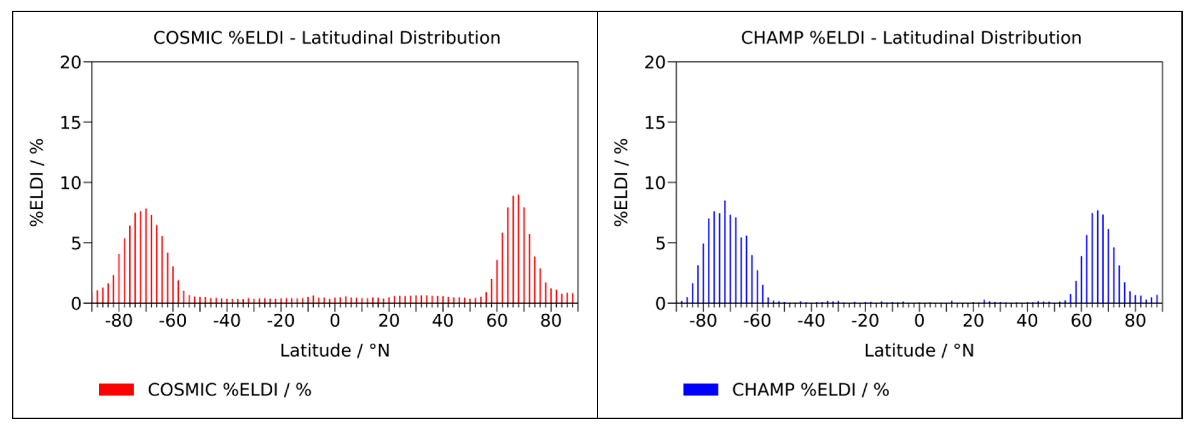
In Figure 3 we present the latitudinal distribution of %ELDI for the entire COSMIC and CHAMP datasets. To create these plots, we first converted the profile’s geographic latitudes into geomagnetic latitudes using the dipole magnetic field model [18]. Then we divided the entire range of latitudes between −90°N to 90°N into 2° wide bins and sorted the profiles into them according to their geomagnetic latitude. As can be seen, both plots show a general increase in %ELDI at auroral latitudes.

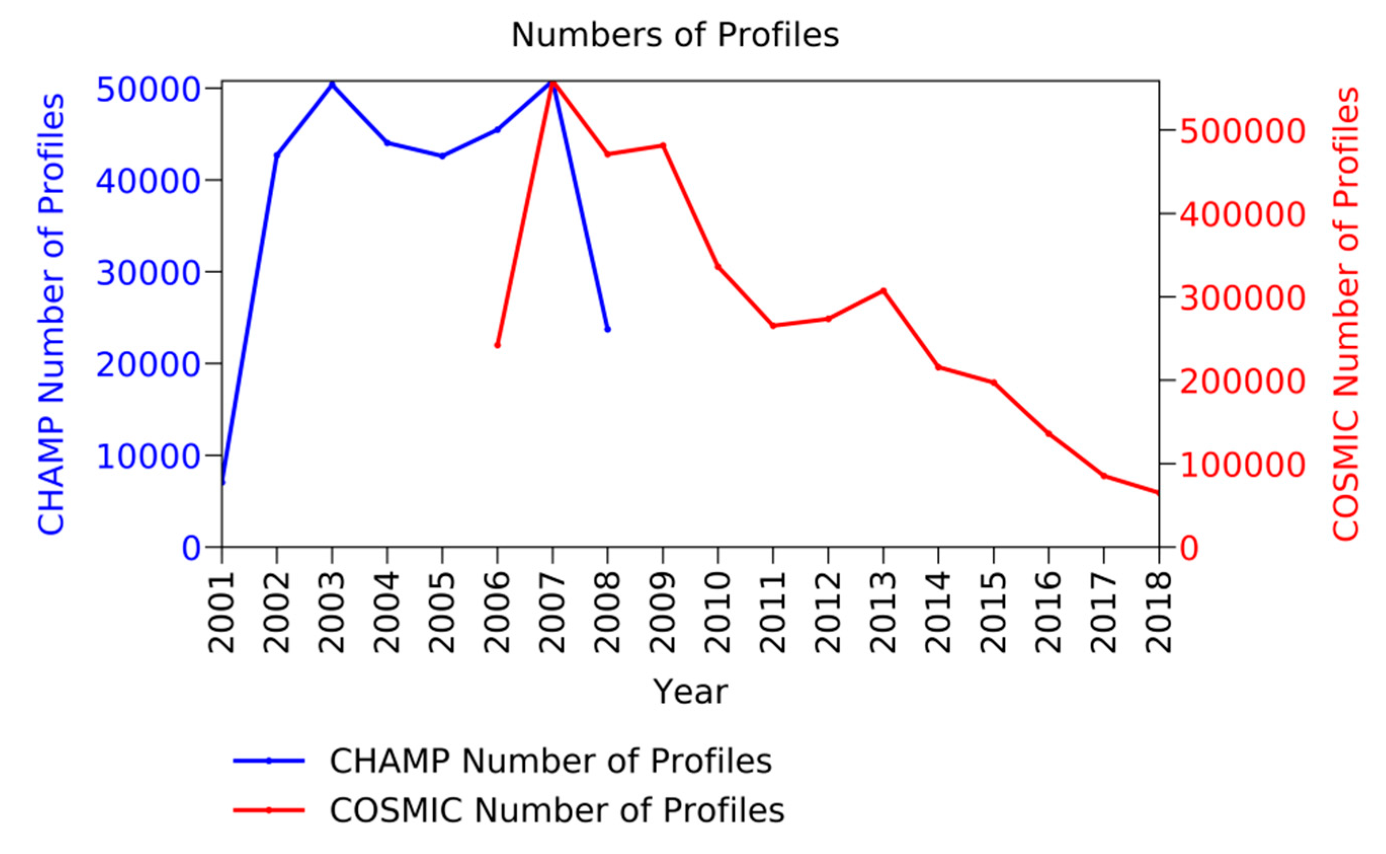
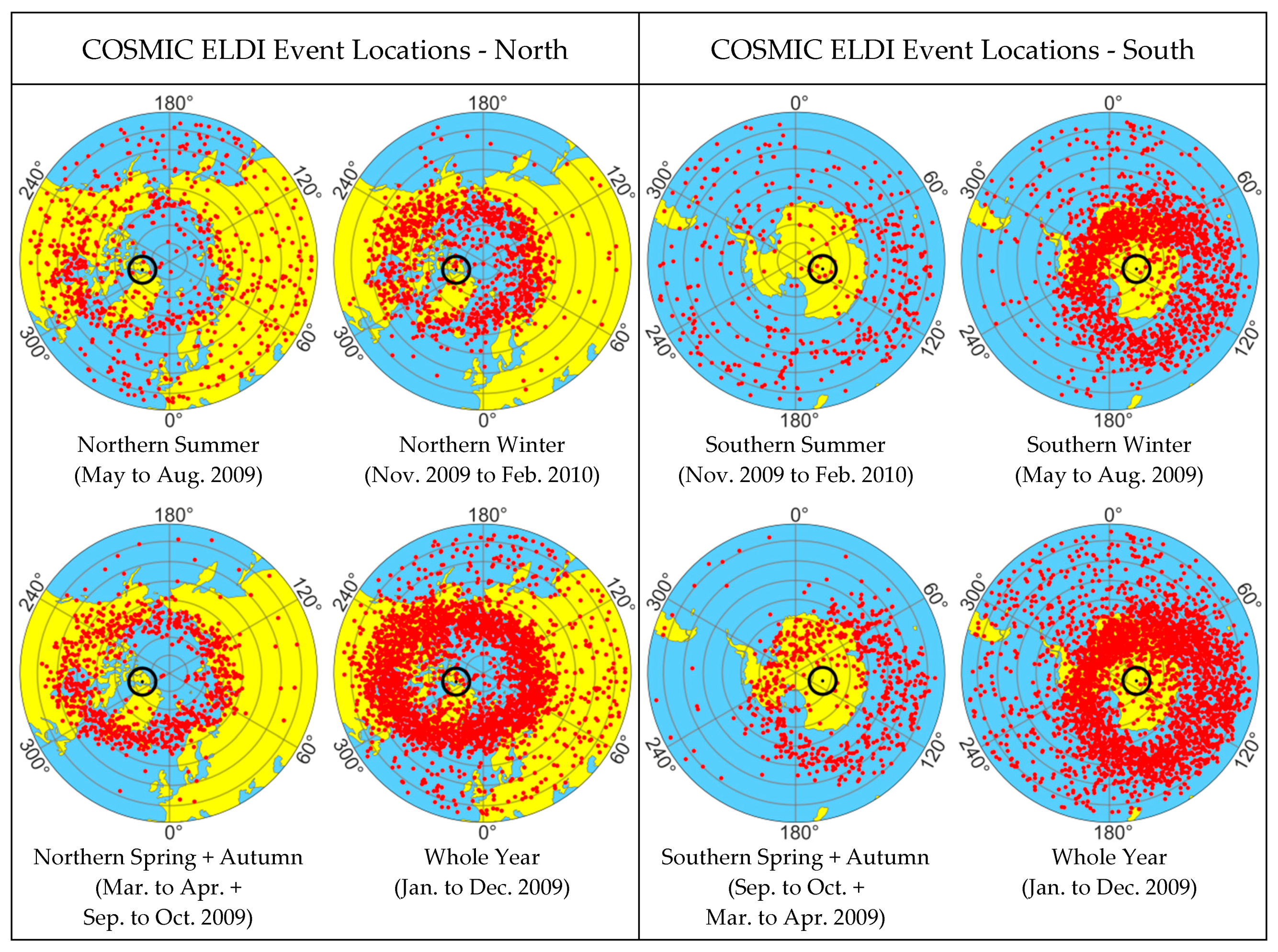
In Figure 4, we show polar maps illustrating the geographic locations of all ELDI events obtained from the COSMIC mission for the high latitude region of the northern hemisphere (45°N to 90°N) and of the southern hemisphere (−90°N to −45°N) as an example for the year 2009. As already shown in Figure 1, the number of electron density profiles retrieved from the COSMIC mission was largest in 2007 and then decreased. At the same time, there also was a solar minimum around 2009. For these two reasons, we expect a large number of ELDI events to occur in 2009, which would be beneficial for visual inspection. The left panel displays the locations of the ELDI events (red dots) for the high latitude region of the northern hemisphere and the right panel for the southern hemisphere. The black circles mark the current locations of the geomagnetic poles as predicted by the IGRF-12 model for the year 2019. These were computed by the World Data Center for Geomagnetism in Kyoto to be (80.6°N, −73.1°E) for the northern and (−80.6°N, 106.9°E) for the southern hemisphere [19]. In both panels, the top left polar map shows the geographic locations of the ELDI events for the summer season and the top right map for the winter season. The lower left map shows their locations for the combination of the spring and autumn seasons and the lower right map those for the whole year. In the maps, we see that in summer only a few and in winter many ELDI events occurred in the auroral regions. During the combination of spring and autumn, the number of occurring ELDI events was between those for summer and winter. Furthermore, we observe for both hemispheres that the ELDI events concentrate along an ellipse located around the geomagnetic pole.

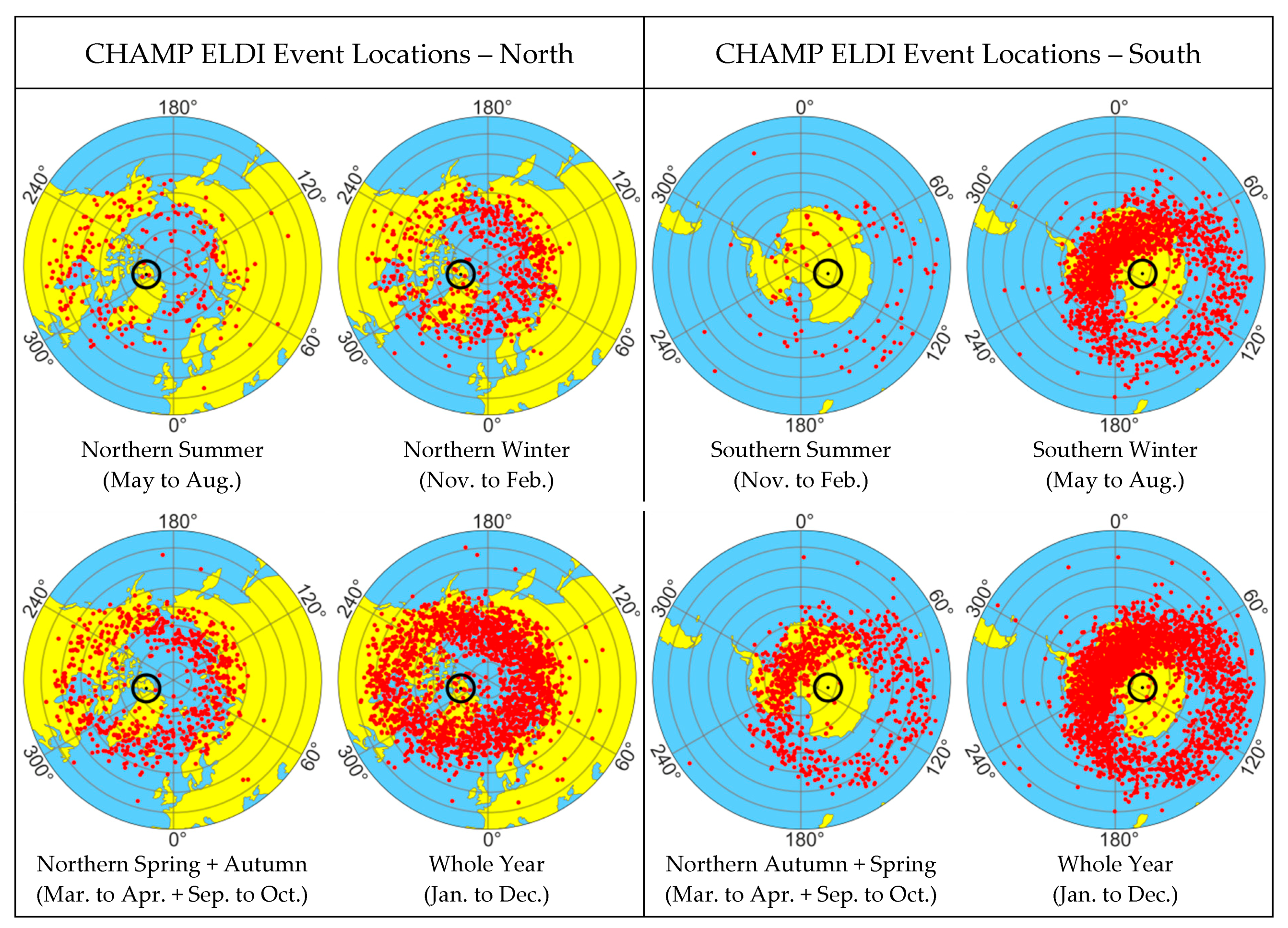
For the CHAMP mission, we created the same kind of polar maps as for the COSMIC mission (Figure 5). Since the size of our CHAMP dataset is only about 1/10th of our COSMIC dataset, we superimposed the data of all years from 2001 to 2008 to improve visual inspection. The maps indicate similar results as for the COSMIC mission.

The polar maps for both satellite missions show an elliptical accumulation of ELDI events, located around the geomagnetic poles. This is in good agreement with the results of Mayer and Jakowski [4]. The finding that the events concentrate in the auroral zones suggests that they are most likely caused by particle precipitation.

3.2. Temporal Variation

3.2.1. Diurnal Variation

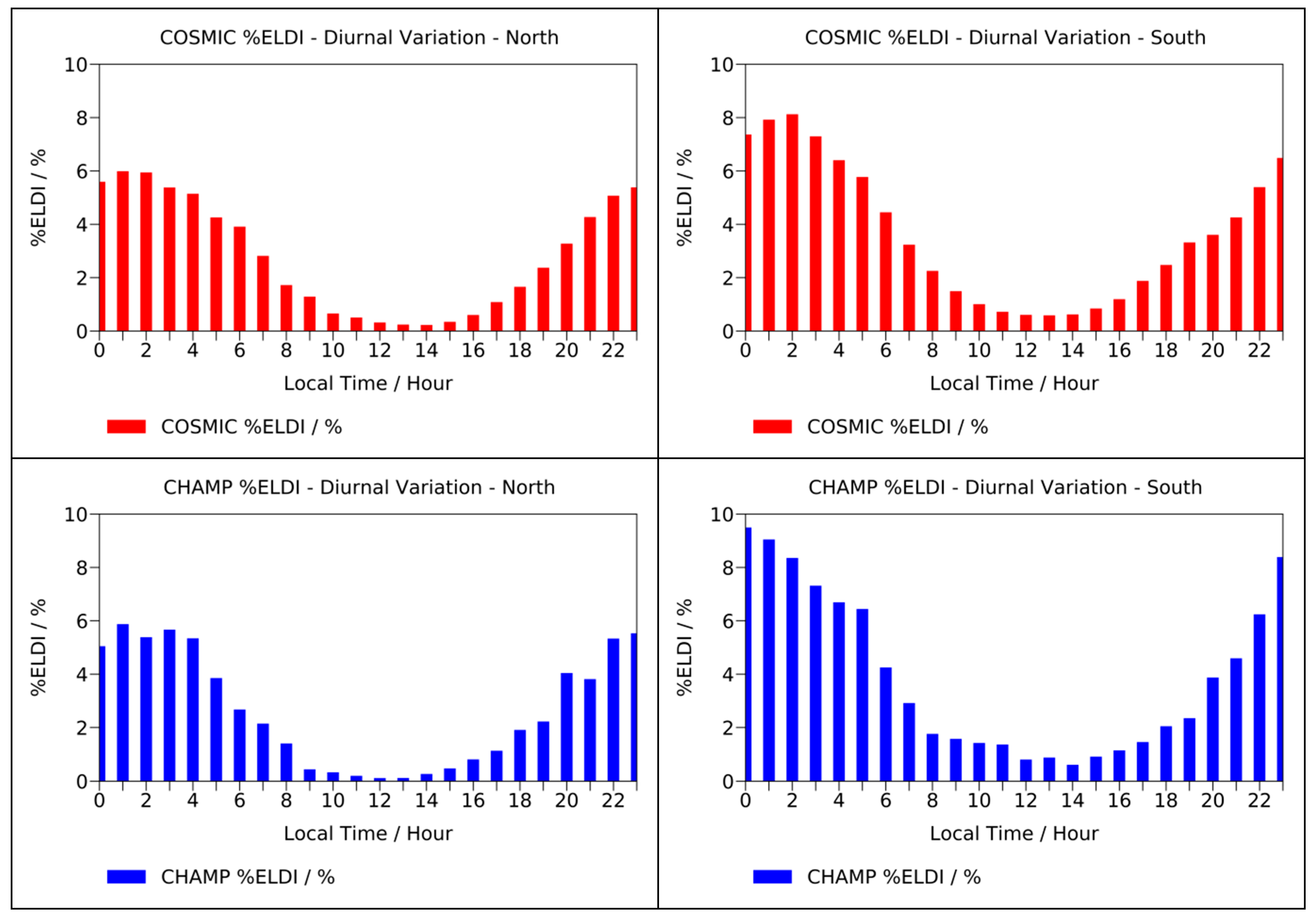
In Figure 6, the diurnal variation of %ELDI, depending on the local time is illustrated for the northern and southern hemispheres. To create these plots, we first selected all those profiles whose geomagnetic latitude fellinto the northern or the southern high latitude region. Then we sorted them into one-hour wide bins based on their retrieval timestamps. The plots reveal that in all cases %ELDI reaches its maximum around local night and its minimum around local noon. This result confirms the findings of Mayer and Jakowski [4], who have also observed an increase in ELDI occurrence during nighttime for the entire northern high latitude region, while Cai et al. [6] have found a similar trend for the EISCAT site. Especially for the COSMIC mission, due to the large amount of profiles, our plots are smoothed out and show a clearly sinusoidal trend over the course of a day.

A probable reason for the observed diurnal variation of %ELDI is the following. The occurrence of ELDI depends on factors that cause the ionization of the E layer to dominate that of the F2 layer. The main reasons for atmospheric ionization are photoionization caused by absorption of solar EUV- and X-rays, particle precipitation, and cosmic rays. Around noon, the low solar zenith angle causes increased photoionization of the sunlit ionosphere. Due to the altitude-dependent variation of the atmosphere’s density and gas composition and the remaining amount of solar radiation, the photoionization of the F2 layer exceeds that of the E layer. Therefore, only a few ELDI events occur during the day. During the night, photoionization is absent, causing the ionization of all layers to decrease due to recombination processes. On the other hand, particle precipitation, which is particularly pronounced on the nightside due to magnetic reconnection processes, causes an additional ionization of the E layer. This increases the probability of nightly ELDI occurrence.

3.2.2. Seasonal Variation

Figure 7 presents the dependency of %ELDI on the month of the year for the northern and southern high latitude regions. Again, the entire COSMIC and CHAMP datasets wereused as a basis to create the plots. The plots show a maximum of %ELDI in local winter and a minimum in local summer. This result fits the findings of Cai et al. [6], who have found out from the analysis of incoherent scatter radar data that more ELDI events emerged in winter and early spring for both the EISCAT and the ESR site.

A possible reason for this result is the following. In winter the average solar zenith angle is larger than in summer, which reduces the proportion of photoionization during the day and thus causes a weaker ionization of the F2 layer. In addition, as winter nights are longer, the ionization of the F2 layer has more time to degrade due to recombination processes at night. The combination of both effects leads to a decrease in the average F2 layer ionization in winter. This increases the probability that the ionization of the E layer induced by particle precipitation becomes apparent and dominates the F2 layer ionization, causing the occurrence of ELDI.

One remarkable feature which can be seen in the plots for the diurnal and for the seasonal variation of ELDI occurrence is the increased magnitude of the %ELDI peak for the southern hemisphere. A cause for this effect could be the elliptic and eccentric shape of the Earth’s orbit, which leads to a varying distance between the Earth and the Sun over the course of a year. In southern summer this distance is smallest (perihelion), causing an increase in the received solar flux. In southern winter it is largest (aphelion), causing a decrease instead. As a result, for the southern hemisphere, this variation in the received solar flux caused by the periodical change in the distance between the Earth and the Sun amplifies the variation caused by the seasonal change in the solar zenith angle. For the northern hemisphere, this relationship causes a reduction of the received solar flux instead. However, the observed asymmetry of %ELDI between both hemispheres requires further study.

3.2.3. Solar Cycle Dependent Variation

Since our COSMIC and CHAMP datasets together cover a long period, we can study the dependency of %ELDI on the 11 year solar cycle. As an indicator of solar activity, we use the F10.7 solar radio flux. The plots in Figure 8 present the relationship between %ELDI and F10.7 for the years 2001 to 2018.

We see a clear trend in the occurrence of ELDI events depending on high and low solar activity. An increase in F10.7 is accompanied by a decrease in %ELDI and vice versa. This is due to enhanced EUV radiation of which F10.7 is a proxy and related stronger photoionization of the F2 layer, which is mostly coupled linearly with F10.7 [20].

3.3. Geomagnetic Storm Dependency

In this section, we investigate the influence of geomagnetic storms on the temporal and spatial distributions of ELDI events. For this purpose, we consider 27 individual storms with Ap < 200 from the period 2001 to 2016. In general, during a geomagnetic storm, we see a sudden drop in Dst, followed by an extended recovery phase. To get the exact hour of the storm’s peak in universal time, we centered a 10 day wide window on each storm date and searched this window for the minimum Dst value. The window width wasarbitrarily chosen, whereby including a relatively large number of days allowed us to also cover the course of longer-lasting storms as completely as possible. By using an even number of days, the windows couldbe symmetrically centered on the peaks, thus equally taking into account both the onset and the recovery phase of the storms.

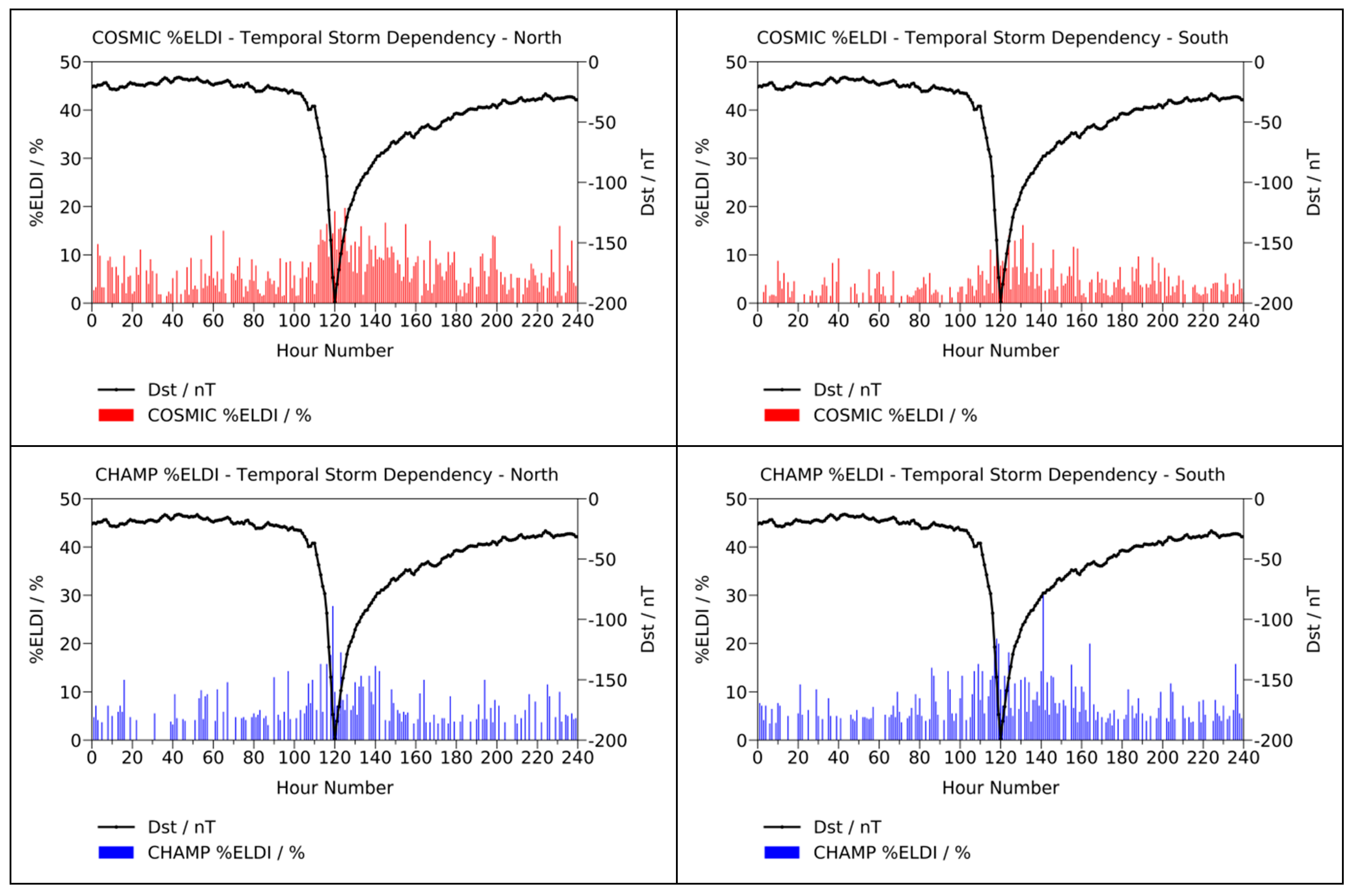
3.3.1. Temporal Variation

In order to examine the variation of %ELDI depending on the temporal course of geomagnetic storms, we first cut out 10 day wide windows from the Dst curve, each of which was centered on one of the previously computed storm peak times. Next, we superimposed all windows and computed the average Dst value for each one-hour wide bin inside of them. We repeated this process for the %ELDI values of the COSMIC and CHAMP missions using the same window sizes and positions as for the Dst case. Figure 9 shows the %ELDI distribution overlaid with the Dst data.

The results indicate that the number of ELDI events increased around the main phase of the storms, i.e., around the Dst minimum. This result correlates with the findings of Mannucci et al. [7], who have also found an increase in the number of ELDI events during geomagnetic storms. A possible reason for the observed variation of %ELDI could be that geomagnetic storms are induced by CMEs or HSSs from the Sun, which are accompanied by an increase in the flow of solar charged particles. These enter the magnetosphere and finally precipitate through the cusp region into the daytime ionosphere and via magnetic reconnection processes into the nighttime ionosphere. This causes an enhanced ionization of the polar E layer, which increases the probability of ELDI occurrence and finally leads to the observed increase in %ELDI during the main phase of geomagnetic storms.

3.3.2. Latitudinal Variation

In this section, we analyze the influence of geomagnetic storms on the latitudinal variation of ELDI events. Figure 10 shows our results in visual form and

Table 2. Mean %ELDI, as well as mean and root mean square (RMS) of the latitudes weighted by %ELDI for the southern (S) and northern (N) high latitude regions.

Mission	Condition	N %ELDI Mean	S %ELDI Mean	N Lat Mean	S Lat Mean	Lat Mean Dist	N Lat RMS	S Lat RMS	Lat RMS Dist
COSMIC	Quiet times	2.90	3.40	68.74°	−69.64°	138.38°	69.15°	70.12°	139.27°
	Storm times	6.35	3.64	67.80°	−68.38°	136.18°	68.13°	69.09°	137.22°
CHAMP	Quiet times	2.29	3.37	68.33°	−70.40°	138.73°	68.61°	70.73°	139.34°
	Storm times	4.15	5.49	67.87°	−70.19°	138.06°	68.31°	70.67°	138.98°

in numerical form. To create the latitudinal plots of the storm times, as shown in the right panels of Figure 10, we evaluated all COSMIC or CHAMP IRO data whose timestamps fellinto a 10 day wide window, centered on any of the previously computed storm peak times. For the latitudinal plots of the quiet times, as shown in the left panels, we evaluated all available IRO data whose timestamps fell outside of these windows instead. We then processed the average %ELDI value for each bin. As can be seen, all plots show a peak in %ELDI located at auroral latitudes, similar to the plot already presented in Figure 3.

Table 2 depicts our results in numerical form. We subsequently computed the mean %ELDI for the northern high latitude region “N” between 45°N to 90°N (column “N %ELDI Mean”) and for the southern high latitude region “S” between −90°N to −45°N (column “S %ELDI Mean”) for the COSMIC and CHAMP missions. We see that in all four cases, the magnitude of %ELDI is higher during storm times than it is during quiet times. This confirms our results obtained in Section 3.3.1, which has shown that geomagnetic storms in principle lead to an increase in the number of ELDI events. Moreover, we computed the mean and the root mean square (RMS) of all latitudes (weighted by %ELDI) that fall into the northern or the southern high latitude regions, respectively. These values are shown in the columns “N Lat Mean”, “S Lat Mean”, “N Lat RMS” and “S Lat RMS”. We then computed the distance between the northern and the southern mean values, respectively RMS values. The results are given in the columns “Lat Mean Dist” and “Lat RMS Dist”.

For both the COSMIC and the CHAMP mission we observe a slight shift of all %ELDI peaks towards lower latitudes during storm times, leading to a smaller distance between the peaks. This observation is in line with the equatorward motion of the auroral zone during geomagnetic storms [21].

4. Conclusions

In the present paper, we evaluated the influence of space weather and geophysical conditions on the occurrence of E layer dominated ionosphere (ELDI) events at high latitudes for the northern and southern hemispheres. As a basis for our investigations, we used a dataset containing almost four million electron density profiles retrieved from COSMIC and CHAMP ionospheric radio occultation (IRO) observations, covering the years from 2001 to 2018. After preprocessing the profiles, in our investigations, we observed elliptic concentrations of ELDI events in the auroral zones, located around the geomagnetic poles of both hemispheres. Moreover, the number of ELDI events has shown an increase at nighttime and during the winter months. Further analyses indicated that the number of ELDI events depends on the solar activity level, increasing during periods of reduced solar activity and decreasing during periods of increased solar activity. In examining the influence of geomagnetic storms, we found an increase in the number of ELDI events during storm times, accompanied by a slight shift of the auroral ELDI distributions towards lower latitudes. Our results confirm and extend the findings of Mayer and Jakowski [4], Cai et al. [6], and Mannucci et al. [7]. Compared to previous work, we did all our analyses utilizing an IRO database that covers a very long period and includes a large amount of electron density profiles, which were obtained from two different satellite missions. Our results obtained for the COSMIC and CHAMP satellite missions and for the northern and southern hemispheres are similar and therefore confirm each other. More detailed studies on the relationship between ELDI and particle precipitation events are planned. It is also planned to complement our database with IRO data from new satellite missions. These missions could benefit from the use of global navigation satellite system (GNSS) receivers with improved data processing and the ability to simultaneously track signals from different GNSS constellations. An example is FengYun-3C, whose GNSS occultation sounder (GNOS) can track four BeiDou Navigation Satellite System (BDS) and six Global Positioning System (GPS) occultation events simultaneously [22,23,24].