Article

Multi-Type Forest Change Detection Using BFAST and Monthly Landsat Time Series for Monitoring Spatiotemporal Dynamics of Forests in Subtropical Wetland

1
School of Information Engineering, China University of Geosciences, Beijing 100083, China
2
ICube Laboratory, UMR 7357, CNRS-University of Strasbourg, 300 Bd Sébastien Brant, CS 10413, F-67412 Illkirch CEDEX, France
3
Key Laboratory of Digital Earth Science, Aerospace Information Research Institute, Chinese Academy of Sciences, Beijing 100094, China
*
Author to whom correspondence should be addressed.
Submission received: 29 November 2019 / Revised: 14 January 2020 / Accepted: 17 January 2020 / Published: 20 January 2020
(This article belongs to the Special Issue Monitoring Forest Change with Remote Sensing)

Abstract

:
Land cover changes, especially excessive economic forest plantations, have significantly threatened the ecological security of West Dongting Lake wetland in China. This work aimed to investigate the spatiotemporal dynamics of forests in the West Dongting Lake region from 2000 to 2018 using a reconstructed monthly Landsat NDVI time series. The multi-type forest changes, including conversion from forest to another land cover category, conversion from another land cover category to forest, and conversion from forest to forest (such as flooding and replantation post-deforestation), and land cover categories before and after change were effectively detected by integrating Breaks For Additive Seasonal and Trend (BFAST) and random forest algorithms with the monthly NDVI time series, with an overall accuracy of 87.8%. On the basis of focusing on all the forest regions extracted through creating a forest mask for each image in time series and merging these to produce an ‘anytime’ forest mask, the spatiotemporal dynamics of forest were analyzed on the basis of the acquired information of multi-type forest changes and classification. The forests are principally distributed in the core zone of West Donting Lake surrounding the water body and the southwestern mountains. The forest changes in the core zone and low elevation region are prevalent and frequent. The variation of forest areas in West Dongting Lake experienced three steps: rapid expansion of forest plantation from 2000 to 2005, relatively steady from 2006 to 2011, and continuous decline since 2011, mainly caused by anthropogenic factors, such as government policies and economic profits. This study demonstrated the applicability of the integrated BFAST method to detect multi-type forest changes by using dense Landsat time series in the subtropical wetland ecosystem with low data availability.

Graphical Abstract

1. Introduction

Dramatic changes have occurred in many wetland ecosystems in the previous decades and have been attributed to the influence of climatic changes and human activities [1]. Research demonstrated that wetland conversion and loss on the global scale has exceeded 50% since 1990 [
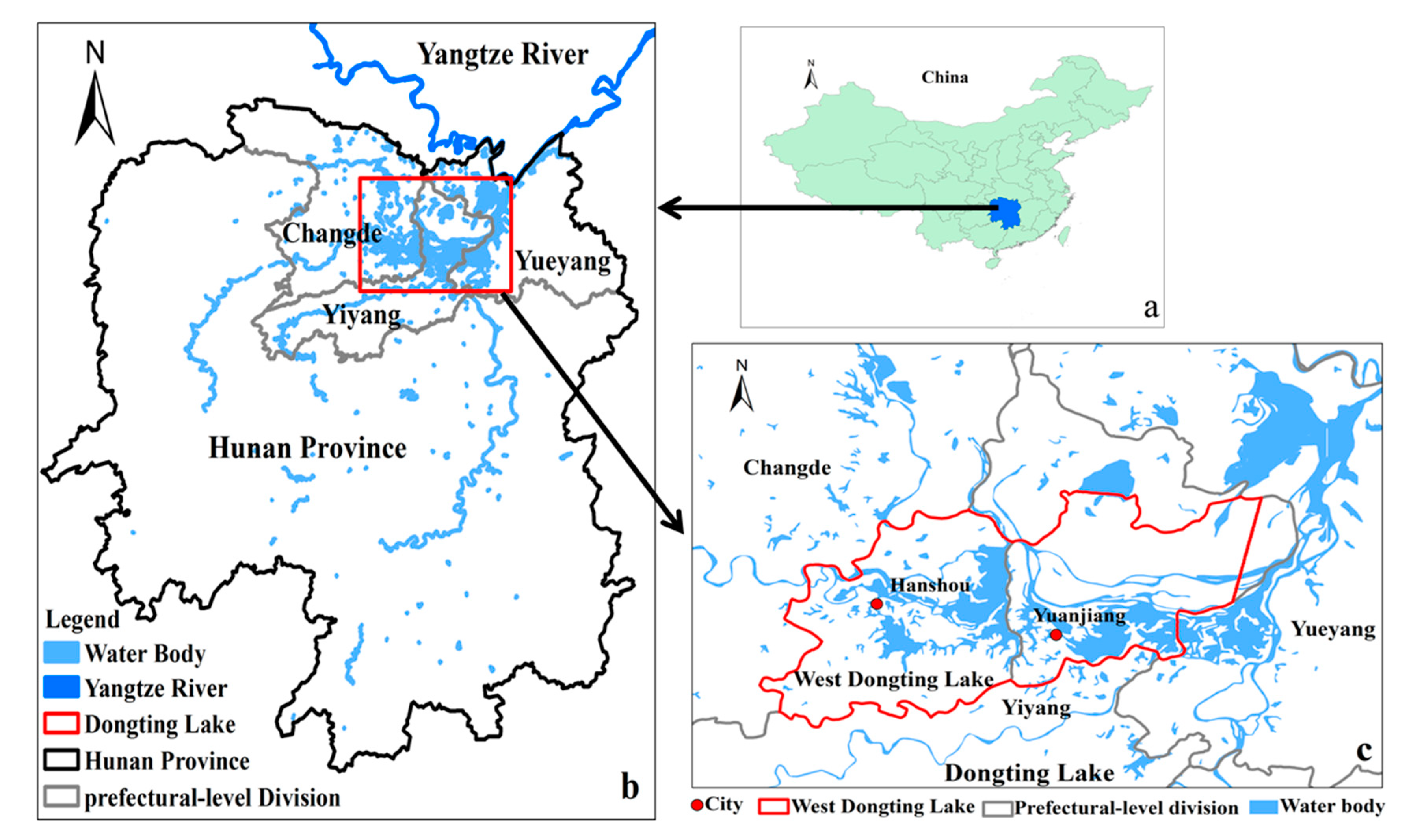
2]. As the second largest freshwater lake in China, Dongting Lake is also one of the important wetland ecosystems. However, the land cover changes, such as land reclamation for developing agriculture and industry, and rapid urbanization have significantly threatened the ecological security of Dongting Lake wetland [3]. With the drop in grain prices and profitable papermaking, a variety of land cover categories, such as paddy fields and bottomland, especially water body, have been transformed to plant the economic forests (i.e., Populus euramericana) for papermaking since the late 1990s. A large number of Populus plantations have accelerated the desiccation of wetland [4], resulting in a decrease of the wetland area [5,6,7]. This situation leads to the death of wetland vegetation [8]; induces biodiversity loss [7]; and influences the community composition [4], structure [7] and function [4] of the wetland ecosystem. Therefore, accurately detecting the land cover changes related to forests and then monitoring spatiotemporal dynamics of forests in the Dongting Lake region are critical for protecting wetland ecosystems.
With the accessibility and accumulation of remotely sensed images on the spatiotemporal scale, remote sensing is a valid alternative for monitoring ecosystem changes. For monitoring spatiotemporal dynamics of forests in the Dongting Lake region with remote sensing, there are the following questions need to be answered: (1) how to accurately detect land cover change? (2) how to acquire the process information of ecosystem change, including land cover change, not just the final results? (3) how to distinguish land cover change from other change types? and (4) how to get the detailed “from what, to what” information on the premise that the land cover change has been identified?
The early common methods, which are quite simple and straightforward, include image differencing, principal component analysis, tasseled cap transform, post-classification comparison, and change vector analysis [9,10,11]. The ideas of these methods are that the changes are generally detected through comparing the difference between the images in two different time phases. Nevertheless, the accuracy of change detection using these methods is dependent on the set threshold [11,12], the availability of ideal images in the same season or the classification accuracy of two images. Another disadvantage of these methods is that the changes are generally detected through comparing the difference between the images in two different time phases without considering the context information in the time dimension, lacking change law and process research [13,14]. Therefore, these methods based on two-temporal images cannot answer questions 1 and 2.
Thus, some change-detection methods based on change trajectories of time series, including Vegetation Change Tracker and Landtrendr, have been developed for studying the change law and process [15,16] and have been widely used for forest disturbances and regrowth monitoring and land cover change detection [17,18,19]. For example, Griffiths et al. employed the LandTrendr and an annual Landsat time series to derive annual forest disturbance maps along with recovery dynamics for answering the question of how the drastic institutional and socio-economic transformation after the collapse of socialism in Romania affected forestry [17]. Kennedy et al. utilized the LandTrendr to detect change and then employed the random forest (RF) classifier (RFC) to label agents of change including urbanization, forest management, and natural change for monitoring habitat in the Puget Sound region, USA [18]. The frequency of time series within these methods is typically one image per year in the same season to minimize seasonal variation and sun angle differences. However, these methods developed at yearly resolution have failed in accurately capturing the timing of the change at the sub-annual scale. This situation results in the detected timing delay of land cover change. Therefore, the optimal result that these methods could provide is generally annual or biennial change [20,21]. Similarly, these methods based on multi-temporal images also cannot answer question 2.
Only the time series with high frequency (e.g., monthly) could describe the entire process of land cover change over shorter time intervals because of the abrupt characteristic of land cover change. Therefore, only change detection with dense satellite time series indeed satisfies the requirement of dynamic monitoring of land cover change [
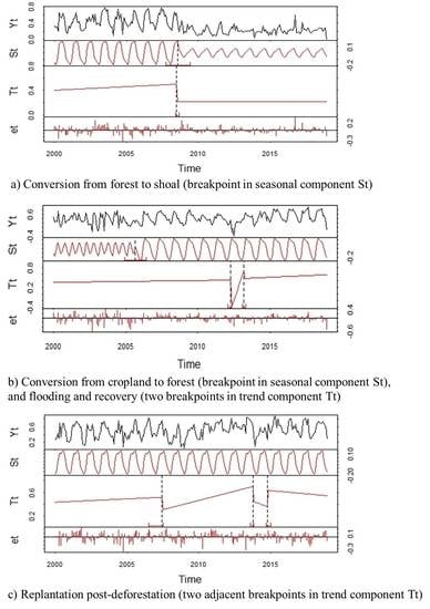
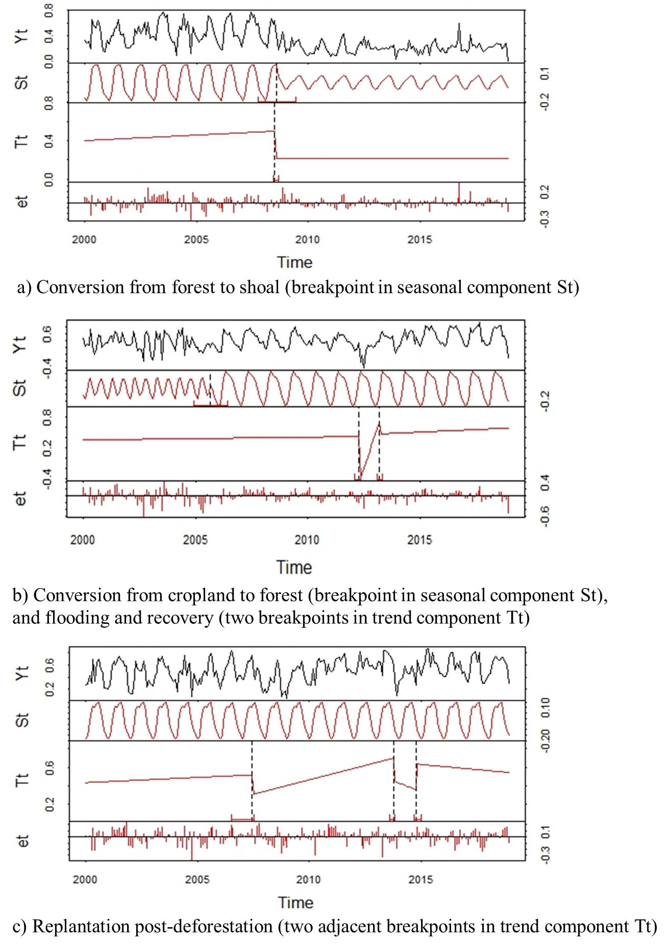
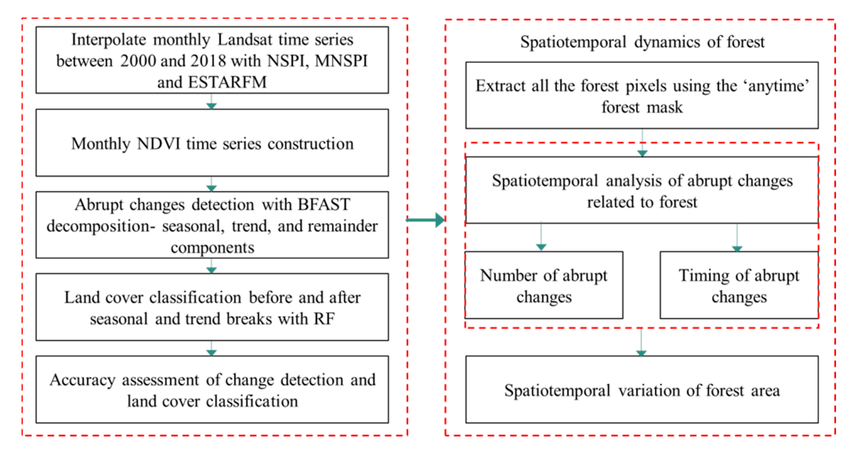
22]. One of the major challenges of change detection with dense time series is to distinguish land cover change from other change types on the premise of minimizing the influences of seasonal phenological variation. The Breaks For Additive Seasonal and Trend (BFAST) meet the challenge through the iterative decomposotion of the time series into trend, seasonal and remainder components [12,23]. The breaks detected in the trend component represent an ephemeral disturbance [24,25], while the breaks detected in the seasonal component represent a land cover change because of the seasonal pattern (phenology) difference between different land cover categories [25,26]. BFAST has been applied in many different land cover categories, such as wetland [24], wildlife nature reserve [25], city [26], tropical dry forest [27], vegetation [28,29], agriculture [30], and abandoned energy development sites [31]. Although BFAST can identify land cover changes (question 1), acquire the process information of land cover change (question 2), and distinguish land cover change from other change types (question 3), it still cannot provide the detailed “from what, to what” information (question 4). Therefore, the land cover categories should be classified before and after abrupt changes while finding the timing and location of land cover change [14,32]. Zhu and Woodcock proposed a continuous change detection and classification (CCDC) algorithm for land cover change detection and land cover categories classification after change detection by using all available Landsat images [21]. The advantage of CCDC is that the coefficients of the fitting time series model and the root mean square error (RMSE) of it are treated as the input parameters of the RFC for land cover classification before and after abrupt changes (question 4).
The Dongting Lake region, in which farmland is one of the major land use categories, is one of the important grain production bases in China. The inter-conversion between farmland and other land cover categories, including forest, frequently occurred because of the policy orientation and economic profit motivation in recent decades. Therefore, the phenological trajectory of all kinds of land cover categories, including farmland with complex intra-annual variations (such as double- or even triple-crop patterns within a year), must be well described for land cover change detection and classification before and after abrupt change. However, the CCDC just adopted a simple sinusoidal model for the phenological trajectory description for a variety of land cover categories, which means it cannot answer any one of four questions in Dongting Lake region with complex change processes [21,33]. Although the BFAST algorithm exhibits difficulty in interpreting the land cover categories before and after the detected abrupt changes, a multi-harmonic model adopted in BFAST could be satisfactory for the complex shape of phenological trajectory and could be applied in the Dongting Lake region. Therefore, BFAST may be feasible for not only detecting the land cover changes related to forest but also classifying the land cover categories before and after abrupt changes by integrating BFAST and classification algorithm.
BFAST is initially proposed to detect change based on high temporal resolution MODIS data, which means it needs dense time series images. However, MODIS data with coarse spatial resolution have the limitation of detecting small changes because of the high fragmentation degree of land cover in the West Dongting Lake region [34]. Lots of medium-resolution data could be freely captured with the Landsat data archive’s opening in 2008. This event enabled change detection with dense remotely-sensed time series at finer spatial resolution [35]. In comparison with the MODIS time series, the Landsat time series possess several advantages, such as higher spatial resolution (30 m) and longer archive (exceeding 47 years), which means more accurate change detection and longer terms of monitoring [36,37,38]. However, the relatively low temporal resolution and frequent cloud cover and shadows result in excessive temporal gaps in the Landsat archive for certain regions or time periods [39], such as the West Dongting Lake region in South China (subtropical region with low optical data availability) in summer. Therefore, for investigating the spatiotemporal dynamics of forest in the West Dongting Lake region with dense Landsat time series by using BFAST, we should answer the new question in this study: (5) how does one acquire the dense Landsat time series with high quality for change detection using BFAST?
This research aims to investigate the spatiotemporal dynamics of forest in the West Dongting Lake region with dense Landsat time series using BFAST through answering five questions. In this research, the timing and location of forest changes, changing types (from forest to what, or from what to forest), and process are acquired by integrating BFAST and classification algorithm. Then the spatiotemporal variations of forest and the potential drivers in the West Dongting Lake region are analyzed on the basis of the information of change detection and classification.

2. Materials and Methods

2.1. Study Area

The Donting Lake region, the second largest freshwater lake and one of the major grain production areas in China, is located in northern Hunan Province (include three prefectural-level divisions of Changde, Yueyang and Yiyang) along the southern bank of the Yangtze River (Figure 1a,b). The major land cover categories in this study area include cropland, water body, forest, shoal (including mudflats, marshland and reed land), and urban (including settlements and roads) in this study area. Land cover changes frequently occurred in this region in recent decades due to natural disasters and human activities. As one of the major land cover categories in this area, the land cover changes related to forest, especially economic forests (i.e., Populus euramericana), are significant. It takes only 3–4 years to make the Populus euramericana with fast growth and strong adaptability grow into useful timber for papermaking. The mass planting of Populus euramericana began in the late 1990s in West Donting Lake (Figure 1c). Many primary and secondary forests, such as Metasequoia and willow, have been replaced by the Populus euramericana. A variety of land cover categories, including farmland and wetland, have been transformed to plant the Populus euramericana due to decline in grain prices and the increasing profitability of paper-making. Parts of the planting areas have disappeared because of flood, urbanization, decline in timber prices, government policy, and construction of the Three Gorges Dam (TGD). As the study area in this work, West Dongting Lake is artificially divided into two parts, namely, the core zone (yellow border in Figure 1d,e) and the transition zone, according to the distance from the main water body and demand for wetland protection (Figure 1d). The core zone includes West Dongting Lake Nature Reserve and buffer zone of the trunk streams flowing into West Dongting Lake. The transition zone, which has some distance from the main water body, is in the adjacent area where some small lakes and tributaries are dispersedly distributed. The value range of Global Digital Elevation Model (GDEM) is mostly from 20 to 40 m in West Dongting Lake, except for the southwestern mountains with GDEM greater than 50 m (Figure 1e).

2.2. Methods

Figure 2 shows an overview of the general workflow followed in this study. The monthly Landsat NDVI time series were generated by using two spatiotemporal interpolation methods named Neighborhood Similar Pixel Interpolator (NSPI) and its modified version MNSPI, and a spatiotemporal data fusion algorithm named enhanced spatial and temporal adaptive reflectance fusion model (ESTARFM). The BFAST was then adopted to detect the abrupt changes with the monthly NDVI time series. The land cover categories before and after abrupt changes were identified through setting the coefficients of the time series model as the input parameters of the RF algorithm. To determine forest extent, we created a forest mask for each image in the time series and merged these masks to produce an ‘anytime’ forest mask for extracting all the forest pixels. After accuracy assessment of change detection and classification, the spatiotemporal distributions of the number and timing of abrupt changes related to forest were analyzed. Lastly, we focused on describing the variation of forest area in West Dongting Lake and discussing the potential drivers. The critical procedures will be introduced in the following sections in detail.

2.2.1. Datasets and Preprocessing

The remotely sensed time series with coarse spatial resolution, such as MODIS and NOAA/AVHRR, are often used for land cover change detection because of their high temporal resolution. However, they have the limitation of detecting small changes because of the high fragmentation degree of land cover in the West Dongting Lake region. Considering the temporal resolution (16 days) of Landsat images and time span of abrupt change and its influence, the time interval between different images in time series is set as 1 month for accurate change detection. Therefore, a monthly Landsat time series with 19 years, from 2000 to 2018, have been adopted for change detection and analyzing spatiotemporal variations of forest in West Dongting Lake region.
Although the Landsat data records were continuously captured from 1972 to present, the relatively low temporal resolution and frequent cloud cover and shadows result in excessive temporal gaps in the Landsat archive for certain regions or time periods [39], such as the West Dongting Lake region in South China (subtropical region with low optical data availability) in summer. Moreover, the permanent failure of the scan-line corrector (SLC) of the ETM+ on Landsat 7 caused approximately 22% of the pixels to be unscanned in ETM+ image since 2003 [40]. In spite of three sensors with 16-day revisit cycle operation, only 197 Landsat images, including 56 TM, 103 ETM+ and 38 OLI, with less than 60% of pixels contaminated by clouds, cloud shadows, and SLC-off gaps were collected in the West Dongting Lake region between 2000 and 2018 (Table 1, Figure 3). The region was not covered by the Landsat images with contaminated pixels less than 60% within 59 months (Table 1). Two spatiotemporal interpolation methods named NSPI for SLC-off gaps filling and its modified version MNSPI for cloud removal were integrated into an iterative process for interpolating gaps pixels and cloudy pixels, respectively [40,41,42]. This method is effective for the time series without extremely persistent clouds, such as the 197 Landsat images with less than 60% of contaminated pixels. However, it is difficult to fill the contaminated pixels with acceptable accuracy when the clouds cover most (over 60%) of the image. Therefore, the missing images in 59 time phases need to be reconstructed in another way to generate a monthly Landsat time series between 2000 and 2018, a total of 228 images (12 scenes per year multiply by 19 years). A spatiotemporal data fusion algorithm named ESTARFM was used to reconstruct the missing Landsat images by fusing available Landsat and MODIS images [43]. Seventy-three MODIS surface reflectance 8-day composite images for data fusion were obtained (Table 2). The ESTARFM uses two pairs of cloud-free fine-resolution Landsat and coarse-resolution MODIS images at base date tm and tn, and one cloud-free coarse-resolution MODIS image at prediction date tp to construct the fine-resolution image at tp. The ESTARFM (1) uses a linear mixture model to establish the relationship between the reflectance of a mixed coarse-resolution MODIS pixel and the fine-resolution Landsat pixels within it at base date tm or tn, and then (2) employs a conversion coefficient to convert the reflectance changes of a mixed coarse resolution pixel to the fine-resolution pixels within it based on spatial and spectral similarity. The missing Landsat pixels at tp are reconstructed based on the two relationships. Either the pair of images at tm or tn can be used as the reflectance at base date to compute the fine resolution reflectance at tp, and a more accurate reflectance at tp can be obtained by a weighted combination of the two prediction results. The validity of the ESTARFM was verified by our previous experiment [44]. After the data reconstruction, NDVI was calculated from Landsat surface reflectance data, considering the NDVI robustness. Finally, an available monthly NDVI time series per pixel with 30-m resolution during this time period for the responding variable in the following change detection process was established.
In addition, the high-resolution images were acquired from Google earth for validation of change detection and land cover classification, and determination of land cover category of each reference pixel with Landsat images together (Table 2). The Advanced Spaceborne Thermal Emission and Reflection Radiometer (ASTER) GDEM data were collected for analyzing spatiotemporal dynamics of forest (Table 2).

2.2.2. Breaks for Additive Seasonal and Trend

BFAST is an iterative algorithm, decomposing time series into three components: trend, seasonal, and remainder components, for change detection [12,23]. The simple form of decomposition model (Equation (1)) is as follows:
Y t = T t + S t + e t ( t = 1 , , p )
where Yt is the observed data at time t, Tt, St, and et, which separately represent the trend, seasonal, and remainder component. p represents the number of observations. Tt can be fitted as the piecewise linear models (Equation (2)) with specific slopes βi and intercepts αi on different m + 1 segments:
T t = α i + β i t ( τ i 1 < t τ i )
where i = 1, …, m, and m represent the number of breakpoints in the trend component. The seasonal component St can be fitted as the piecewise harmonic models (Equation (3)) on different n + 1 segments:
S t = k = 1 K [ γ j , k s i n ( 2 π k t f ) + θ j , k c o s ( 2 π k t f ) ] ( τ j 1 # < t τ j # )
where j = 1, …, n, and n is the number of breakpoints in the seasonal component. Variable k is the order of harmonic function and its set as 3 to more accurately detect complex phenological changes, such as double- or even triple-crop patterns within a year in this study area. As a result, not only the land cover categories with simple phenology patterns, such as forest with yearly phenological cycle, but also those with the complex phenology patterns could be accurately described and then classified. The frequency f is set as 12 for annual observations for a monthly Landsat time series in this research.
The iteration process is initialized by estimating the seasonal component S ^ t through utilizing the seasonal-trend decomposition (STL) algorithm [48]. First, the residual-based moving sum (MOSUM) test [49] is used to test whether breakpoints τ* 1, …, τ* m occur in the adjusted trend component Yt S ^ t . The position and number of breakpoints in the trend component are then determined through minimizing the Bayesian Information Criterion (BIC) [50] and the residual sum of squares (RSS), respectively. Then robust regression on the basis of M-estimation [51] is used to estimate coefficients α and β in the trend component for each segment, and the trend estimate T ^ t is computed on the basis of Equation (2). Similarly, the MOSUM test is utilized to test whether breakpoints τ# 1, …, τ# n occur in the de-trended seasonal component Yt T ^ t , and the minimization of the BIC and RSS is conducted to determine the position and number of the breakpoints in the seasonal component. Coefficients γj,k and θj,k of the seasonal component in Equation (3) for each segment are also estimated on the basis of M-estimation, and then the seasonal estimate S ^ t is computed on the basis of Equation (3). The above steps are iteratively performed for breakpoint detection and parameter estimation until the number and position of detected breakpoints remains stable.
Considering the frequent land cover changes that have resulted from the active human activities in this study area, we set 1 year as the minimal segment size between successive abrupt changes for fine change detection. Both changes will be detected as long as their interval exceeds 1 year.
The phenological characteristics among land cover categories are different, and they can be effectively captured by the seasonal component. The breakpoint in the seasonal component, which means the phenological change before and after breakpoint, suggests a potential land cover change. In this study, land cover changes related to forest, including conversion from forest to other land cover categories (hereinafter referred to as FTO) and from other land cover categories to forest (hereinafter referred to as OTF), are detected. Results calculated by using BFAST in sample areas of forest, an area converted from forest to shoal (Figure 4a) or from cropland to forest (Figure 4b), indicate the phenological characteristic differences among different land cover categories. Although the forest and shoal have a significant cyclic intra-annual variation with one peak in each year, the seasonal component of the shoal possesses small fluctuations of intra-annual NDVI values. Cropland has an intra-annual variation with two peaks in each year compared with the phenological characteristic of one peak within 1 year for forest. The breakpoints in the seasonal component indicate the structural change of the phenological characteristic and therefore suggest a permanent land cover change. Specifically, the monthly NDVI time series decomposed by BFAST can detect the land cover changes related to forest in the subtropical wetland.
The short-term disturbances, such as flooding and replantation post-deforestation, result in conversion from forest to forest (hereinafter referred to as FTF). Although these ephemeral changes, including disturbance to forest and then recovery performed within a short term, could not result in the permanent change related to forest, such as the land cover change (FTO or OTF), they still cause short-term forest change and spatiotemporal variation of forest. Therefore, the description of flooding and replantation post-deforestation is as important as the detection of land cover changes related to forest for monitoring the spatiotemporal variation of forest in West Dongting Lake. Results calculated by using BFAST over sample areas of forestland, an area flooding (Figure 4b), or replantation post-deforestation (Figure 4c), showed that these interruptions only cause abrupt changes in the trend component. Two breakpoints (dash lines in Figure 4) closely adjacent to each other in trend component represent the disturbance (the former) and recovery (the latter), respectively. The major difference between flooding and replantation post-deforestation is whether the value of NDVI time series is greater than zero when the disturbance occurred. These results showed that the different ephemeral disturbances, even the recovery process, could also be detected and distinguished by BFAST.

2.2.3. Land Cover Classification after Breakpoint Detection

BFAST could identify abrupt change types in the remotely sensed time series: Abrupt changes in the seasonal component indicate a permanent land cover change; the ephemeral changes, such as flooding and replantation post-deforestation, could be detected in the trend component. However, land cover categories before and after the breakpoints could not be identified by using the BFAST algorithm. Similar to the CCDC algorithm, the coefficients of the time series models (Equations (2) and (3)) fitted by BFAST are used as input parameters to RFC [52] for land cover classification, which is the main reason why the monthly Landsat time series and BFAST are adopted in this study. The subsequent classification after change detection could also reduce the pseudo change (false positive in change detection). Therefore, the land cover categories at any given time and location could be effectively acquired by integrating BFAST and RF algorithms.
Each pixel has its own time series models (the trend model in Equation (2) and seasonal model in Equation (3)) before and after any breakpoint. For example, n + 1 time series models exist when n breakpoints are detected in the seasonal and trend components by BFAST. Given that each land cover category has its own specific shape of the time series models [53], the coefficients of each time series model used to describe the shape could be utilized as input parameters to the trained RFC for classifying land cover category. Accordingly, the land cover category of each pixel for each time series model in the entire period is determined. Two coefficients (α and β in Equation (2)) in the trend component and six coefficients (γk, θk, and K = 3 in Equation (3)) in the seasonal one were selected as the classification features in this study. Variable α represents the overall NDVI value of each time series model, and β indicates inter-annual differences, the combination of which describe the mean value and inter-annual trend of each land cover category. Meanwhile, γk and θk provide information about intra-annual seasonal change pattern primarily caused by phenological change.
The land cover reference data for classification, a total of 26,137 reference pixels for five land cover categories, were collected on four dates within the period covered by the Landsat time series (Table 3). An approximately equal number (around 6500) of reference pixels were collected on each date. The number of reference pixels for different land cover categories on each date is different, considering the difference among areas, intra-class heterogeneity and data availability of each land cover category. The land cover category of each reference pixel at the given time was determined through careful visual interpretation by using the Landsat time series and the images with high spatial resolutions from Google Earth; and the reference pixels of each land cover category are equably collected at representative regions. Random sampling with replacement design was used to divide the land cover reference data into two parts of training data (for training the classifier) and test data (for validating the classifier) with sampling probabilities of 0.7 and 0.3, respectively.

2.2.4. Accuracy Assessment

Due to the lack of remotely sensed images with higher temporal and finer spatial resolution than Landsat images over the last few decades covered by Landsat, the primary and optimal source for accuracy assessment of long-term change detection using historical dense time series of Landsat is the Landsat images themselves [21,54,55,56]. Meanwhile, the images with high spatial resolution from Google Earth could help manually interpret the land cover categories and change. A random stratified sample design proposed by Zhu and Woodcock [21] was used to assess the detection accuracy in this study. A total of 600 reference pixels were selected. Three hundred example pixels represent the areas where forest was persistent between 2000 and 2018 and another 300 pixels represent those where forest change occurred, which were identified by the BFAST and RF algorithm. In each pixel, we visually examined the NDVI time series data and images with high spatial resolution acquired from Google Earth to determine whether and when forest change occurred for that specific location.
A randomly selected subset, a total of 30% (7837 reference pixels) of the land cover reference pixels, were used to assess the accuracy of classification with the RF algorithm (Section 2.2.3). A confusion matrix was produced to estimate user’s and producer’s accuracy of each land cover category, and overall accuracy.

2.2.5. Spatiotemporal Dynamics Analysis of Forest

Eleven indicators were utilized to analyze the spatiotemporal dynamics law of forest in West Dongting Lake region from the aspect of duration, number and timing of abrupt change, and areas (Table 4). Df is used to measure the duration of forest plantation within each pixel between 2000 and 2018. Two indicators (Ps, Pc) are utilized to measure the proportion of stable and changed forests, respectively. Nc(i), Pc(i) are separately used to measure the number and proportion of changed pixels with different numbers of abrupt changes. ML is calculated to illustrate the proportion of abrupt changes in each region, while two indicators (iK, RL) are adopted to describe the change frequency of each forest pixel and each region, respectively. Tl and APK,T are utilized to describe the timing of the last abrupt change and the annual proportion of all abrupt changes, respectively. In the end, forest areas AL,t in every time phase within time series are calculated. Five indicators (Ps, Pc, ML, RL, AL,t) are calculated in each region, while six indicators (iK, Nc(i), Pc(i), ML, Tl, APK,T) are calculated based on different change types.

3. Results

3.1. Accuracy Assessment

3.1.1. Accuracy Assessment for Change Detection

For changed pixels, the results showed the producer’s accuracy of 90.7% and user’s accuracy of 84.3% (Table 5). For stable pixels, the results showed the producer’s accuracy of 85.4% and user’s accuracy of 91.3%. The change detection with an overall accuracy of 87.8% indicated that the changes related to forest were well captured by BFAST algorithm. The accuracy of the timing of change detection was further assessed for 253 reference pixels in which the change was identified with the Landsat time series data or high spatial resolution images acquired from Google Earth and correctly detected by BFAST (Table 6). The proportion of pixels in which the change timing detected by BFAST is the same as that identified with reference data is 77.47%. The proportions of the pixels in which the detected timing is later than that identified with reference data within 2 months or over 2 months are 13.04% and 9.49%, respectively. If we consider that the actual date of change is within a quarter of a year of the detected change date, the accuracy of timing is as high as 90.51% (77.47% + 13.04%).
The reference Landsat images before and after abrupt change and results of change detection with BFAST for each conversion type were displayed to further intuitively illustrate the algorithm ability (Figure 5). A typical area converted from forest to urban in 2008 was found by BFAST algorithm, in which wavelet characteristics of the seasonal component were weakened to a small fluctuation of intra-annual NDVI values after the breakpoint (Figure 5a). The slow urban expansion resulted in partial forest cut within the pixel, in which this spectral change was insufficiently large to be detected by the BFAST algorithm until it was totally changed. Accordingly, the timing of change detected by BFAST was a little later (2 months) than the actual timing observed from the reference data. Another typical area converted from shoal to forest in 2005 was also found by BFAST algorithm, in which the land cover before and after breakpoint and breaking time detected by BFAST and RF algorithms could correspond to those acquired from the reference Landsat images (Figure 5b). Intra-annual changes, such as the flooding and replantation post-deforestation, were difficult to be detected by algorithms, such as Landtrendr, with the frequency of time series of one image per year. The accuracies of flooding and replantation post-deforestation detected by BFAST algorithm were high compared with the reference Landsat images before and after the breakpoint (Figure 5c,d). Moreover, the confidence interval of each detected breaking time (two dashed lines in the trend component) was narrow.

3.1.2. Accuracy Assessment for Classification

The overall accuracy and Kappa coefficient of the land cover classification with five categories are 92.96% and 0.9026, respectively (Table 7). Not only producer accuracies but also user accuracies for the different land cover categories are mostly greater than 90%. These results indicate that the RF classifier is sufficient for classifying the land cover categories in Dongting Lake region. The largest confusion is between forest and shoal, with the producer accuracy for shoal being 73.44%. The possible reason is that other vegetation growing in shoal, such as the annual shrubs or herbs, are similar to forest in the spectral characteristics at the spatial resolution of 30 m.

3.2. Spatiotemporal Dynamics of Forest

3.2.1. Duration and Spatial Distribution of Forest Plantation

Previous studies mostly focused on the regions that are known to have been forested at the beginning of the first monitoring period and neglected the forest regions in which the forest has not been planted in the initial period [27,57], such as the pixels, the land cover of which changed from another land cover category in the initial period to forest in the later period. Considering the characteristic of frequent change between forest and the other land cover categories in West Donting Lake, we created a forest mask of each image in the time series and merged these masks to produce an ‘anytime’ forest mask for extracting all forest pixels. The distribution map of the duration proportion of forest plantation between 2000 and 2018 (Df, Table 4) is shown in Figure 6. The forests are mainly distributed in the core zone surrounding the water body and southwestern mountains. The Df of most forest regions is 1 (stable forests), whereas the rest of the forests, the Df of which are less than 1 (changed forests), are dispersedly distributed. Especially, the forest areas with Df less than 0.5 are mainly distributed in the south of the West Donting Lake region, and most changed forests with Df greater than 0.5 are concentrated in the core zone. In contrast with the forests in South China, which are mainly distributed in mountainous regions because of the limited flatlands with low elevation utilized for croplands or settlements, a large part of forests in the West Dongting Lake region are distributed in the flatlands with low elevation, except for the forests in the southwestern mountains (Figure 1e and Figure 6).
Further comparison of the spatial distribution between stable and changed forests for each DEM range and region showed considerable differences (Table 8). The proportions of stable and changed forests (Ps and Pc, Table 4) are 72.08% and 27.92% for all forest regions, a total of 1,180,893 forest pixels. Over 60% (44.45%/72.08% = 61.67%) of the stable forests are distributed in the transition zone, including those with DEM greater than 50 m (27.55%); the stable forests in the core area are mainly distributed in the region with DEM ranging from 20 to 40 m. This finding indicates that the stable forests are mainly distributed in relatively high elevation regions of the transition zone and low elevation regions of the core zone. The proportion of changed forests with DEM ranging from 30 to 40 m is the highest (11.12%), and those with DEM ranging from 20 to 40 m is over 60% of the changed forests, especially including those in the core zone. In addition, the proportion of changed forests in the transition zone with DEM greater than 50 m is also high (6.88%). These results showed that the changes related to forest were mainly detected in the low elevation region surrounding the water body and relatively high elevation region of the transition zone. Although the proportion of forests in the core zone (11.69% + 27.63% = 39.32%) is lower than that in the transition zone (16.23% + 44.45% = 60.68%), the proportion of changed forests in all of the forests in the former (11.69%/39.32% = 29.73%) was slightly higher than that in the latter (16.23%/60.68% =26.75%). Meanwhile, the proportion of changed forests in the region with each DEM range decreased with the DEM increase. These results further showed that the forest changes in the core zone and low elevation region are more prevalent.
All the forest pixels were extracted by using the ‘anytime’ forest mask, and then the proportion and spatial distribution of stable and changed forests were also analyzed in this section. However, the spatiotemporal characteristic of forest changes must be analyzed to further explain the variation characteristic of forests. Therefore, the number and timing of abrupt changes related to forest, and the variation of forest areas will be discussed in the following sections.

3.2.2. Number of Abrupt Changes Related to Forest

The number (Nc(i), Table 4) and proportion (Pc(i), Table 4) of pixels with single (or multiple) occurrence(s) (iK, Table 4) of abrupt change for each change type were compared to show considerable differences (Table 9). In all the changed pixels related to forest (27.92%), the number of abrupt changes of 25.35% out of 27.92%, which exceeds 90% (25.35%/27.92% = 90.80%) of all the changed pixels related to forest, is from 1 to 3. The number of FTO and OTF, which separately occurred in 13.36% and 11.89% of the forest pixels, is basically 1. The proportion of the forest pixels with FTF is 15.70%. In contrast with FTO and OTF, the proportion of forest pixels with one time FTF (flooded or replantation post-deforestation) is generally equal to that with multiple times FTF. Results indicated that not only the proportion of forest pixels with FTF but also the number of FTF is higher than those of FTO and OTF.
The distribution map of the number of breakpoints is shown in Figure 7. Most areas with two or more times changes are in the core zone surrounding the water body, and the areas with one change are dispersedly distributed in the whole study area, especially the southwest mountains (Figure 7a,b). FTO or OTF, the number of which is generally 1, are principally distributed in the areas surrounding the water body (Figure 7c–f). The distribution of areas with different numbers of FTF is almost the same as that with the estimated number of all abrupt changes (Figure 7g,h).
The number of abrupt changes is summarized for each DEM range and region to facilitate further comparison (Figure 8). Most changes occurred in the areas with DEM ranging from 20 to 40 m, the proportion (ML, Table 4) of which in all of detected changes is over 65% (Figure 8a). In these areas with DEM ranging from 20 to 40 m, the proportion of detected changes in the core zone is higher than that in the transition zone regardless of the change types (Figure 8b–d). The detected changes in the region with DEM over 40 m are generally distributed in the transition zone, the proportion of which is much less than that with DEM ranging from 20 to 40 m. This is because the elevation in West Dongting Lake is generally less than 40 m and the main land cover categories in the transition zone with DEM less than 40 m are cropland and settlement (Figure 1 and Figure 6). The proportion of OTF (18.59%) and FTO (18.59%) in the transition zone with DEM over 50 m (southwest mountains) is relatively low compared with the proportion of OTF (42.89%) and FTO (42.78%) in the core zone with DEM less than 40 m (Figure 8b,c). The proportion of FTF in the southwest mountains (24.64%) is also lower than that in the core zone with DEM less than 40 m (43.33%; Figure 8d).
The ratio (RL, Table 4) of the total number of changes to the total number of changed forest pixels was proposed to further reflect the frequency of forest change in different regions. Although the proportion of change number in the core zone is slightly less than that in the transition zone (47.49% versus 52.51% of 665,744), the ratio in the core zone (2.29) is higher than that in the transition zone (1.82) considering the proportion of the changed forests in both zones (11.69% versus 16.23% of 1,180,893, Table 8). Moreover, the ratio in the core zone is slightly higher than that in the transition zone regardless of the change types, especially FTF (2.15 versus 1.66). Specifically, the proportion of changed forests (Section 3.2.1) and the ratio in the core zone are higher than those in the transition zone. This finding further indicates that the forest change in the core zone is more frequent than that in the transition zone.

3.2.3. Timing of Abrupt Changes Related to Forest

The spatial distribution of the timing (Tl, Table 4) of the last abrupt change detected from the monthly NDVI time-series is shown in Figure 9. Most FTO in the core zone occurred between 2011 and 2015, whereas that in the transition zone is between 2012 and 2017 (Figure 9a,b). The major years of OTF in the core zone region are 2000, 2012, and 2016, while most transition zones had OTF in 2012, 2016, and 2017 (Figure 9c,d). FTF mainly occurred in 2017 for the southwest mountains, while large parts of the core zone region had FTF between 2006 and 2017 (Figure 9e,f).
In contrast with the analysis of the timing of last change in Figure 9, the timing of all changes was summarized each year (APK,T, Table 4) to facilitate further comparison (Figure 10). Large parts of FTO occurred since 2011, while a relatively low proportion of FTO was detected before 2011 (Figure 10a). Several clear peaks of OTF were detected during 2000, 2012, 2016, and 2017 (Figure 10b). The frequency distribution of the timing of FTF was relatively even for each year from 2000 to 2018, except for one peak in 2017 (Figure 10c).

3.2.4. Variation of Forest Areas

The spatial distribution of forest pixels and the forest areas (AL,t, Table 4) at any given time could be effectively acquired with the application of integrating BFAST and RF algorithms to the monthly NDVI time series (Figure 11). The variation of forest areas in West Dongting Lake experienced three steps (Figure 11a): a rapid expansion of forest plantation from 2000 to 2005, except for a small drop between 2001 and 2002; the forest areas were relatively steady from 2006 to 2011, except for one valley in 2008; the forest areas continued to decline since 2011.
The increased forest areas in the core zone are significantly higher than that in the transition zone during the period of 2000 through 2005 (Figure 11b). This finding indicates that forest plantation in the core zone is the major contribution for increased forest areas between 2000 and 2005. However, the increasing rate of forest area in the transition zone is higher than that in the core zone since 2003. The forest areas in the core zone generally remained steady between 2003 and 2011. The forest areas in the transition zone first also had the same trend as that in the core zone between 2006 and 2008 and then increased between 2008 and 2011. The overall trend of the forest areas in the core zone began to fall since 2011, except for the forest areas in the core zone sharply fluctuating in 2014 and 2016. The forest areas in the transition zone began to fall since 2013, which is laggard compared with the downtrend in the core zone; the decreasing trend and rate of forest areas in the transition zone almost did not change. The forest areas in the core zone sharply decreased during 2017. By contrast, the forest areas in the transition zone showed an increasing trend in 2017.

4. Discussion

The accuracy assessment results of change detection show higher user accuracy for stable pixels and higher producer accuracy for change pixels (Table 5), indicating more commission errors than omission errors in the detected change pixels. The errors are possibly due to the following reasons: (1) noise; (2) partial change; (3) and influence of classification accuracy. Although the validity of the NSPI, MNSPI and ESTARFM are verified in this study and our previous experiment [44], the noise cannot be removed completely, which is mistakenly detected as change (commission error). The partially changed pixels are difficult to be detected by BFAST due to the insufficiently large spectral change (omission error). The similarity between shoal covered by other vegetation and forest in the spectral characteristics within the Landsat image with 30 m resolution may result in misclassification, and then the inter-conversion between them cannot be identified even if the conversions have been detected by BFAST before classification (omission error).
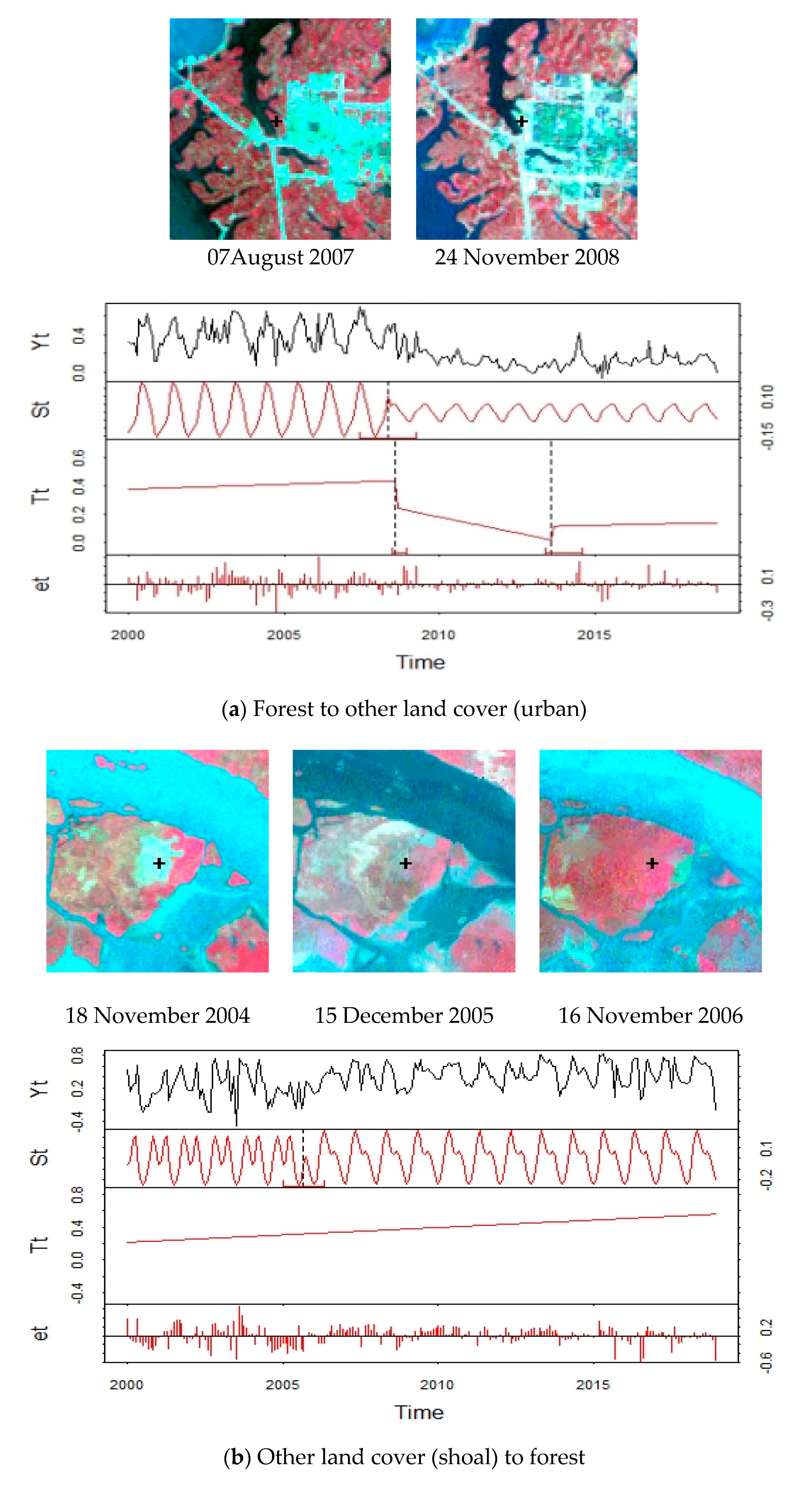
The timing errors of change detection are possibly due to the following reasons: (1) slow change; (2) reconstruction effect of time series; and (3) parameter setting of BFAST. As shown in 
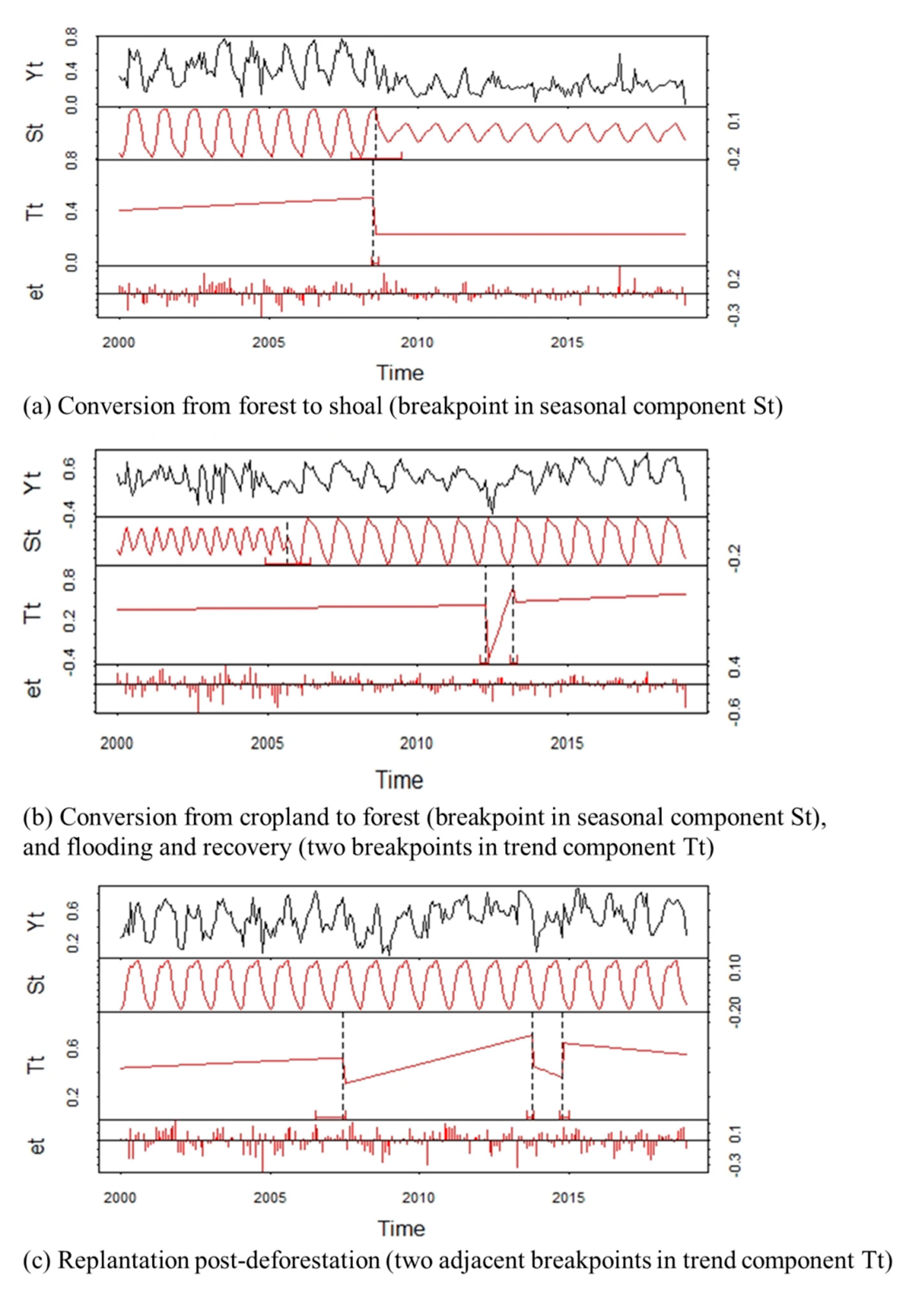
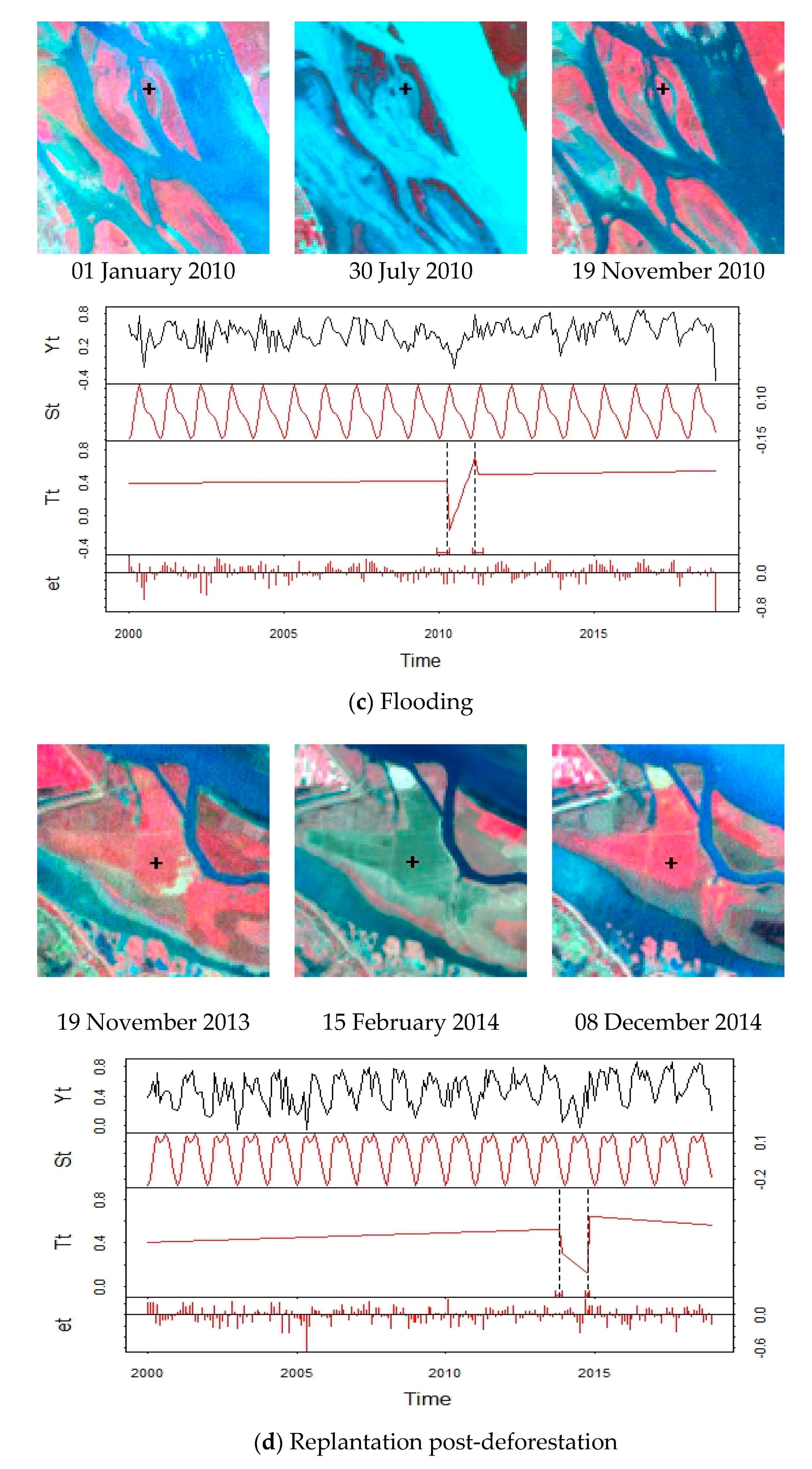
Figure 5a, the slow urban expansion resulted in a partial forest cut within the pixel, in which this spectral change was insufficiently large to be detected by the BFAST algorithm until it was totally changed. Accordingly, the timing of change detected by BFAST was a little later (2 months) than the actual timing observed from the reference data. NSPI, MNSPI and ESTARFM algorithms interpolated the contaminated pixels and reconstructed the missing images without considering possible land cover change at that time phase, which means that the land cover category of the interpolated or reconstructed pixel with actual land cover change may have mistakenly remain unchanged at that time phase. This situation may have resulted in the land cover change detected timing delay of one or several months. We set 1 year as the minimal segment size between successive change detections in BFAST to reduce pseudo changes. However, this strategy caused the interval of two breakpoints closely adjacent to each other in the trend component, representing the short-term disturbances (such as flooding and replantation post-deforestation), to be just 1 year. In fact, the cycle of the short-term disturbances is generally less than 1 year, and it may delay the timing of the recovery process.
On the basis of the error analysis, there are some feasible strategies as follows: (1) change detection through integrating temporal and spatial information and (2) classification using deep learning. Similar to most change detection methods utilizing time-series data, the BFAST adopted in this study is mainly focused on the information on the temporal domain and independently processes each pixel, without considering the change characteristics generated on the spatial domain [14,58]. This results in the accuracy of change detection relying heavily on the quantity and quality of time-series data in the temporal domain, such as the reconstruction accuracy of the monthly Landsat time series in this study. In fact, the change essentially occurs in the spatial domain and is reflected in the temporal domain, in other words, change determines the necessity of defining ‘time’ by human. Therefore, time series analysis based on an independent pixel is insufficient to accurately and roundly describe a series of change characteristics. Several algorithms recently eliminated the noise and other change (such as seasonal change) interference through integrating spatial information, which improved the change detection accuracy [18,59,60,61,62]. These methods have less reliance on the quantity and quality of time-series data. For example, Hamunyela et al. used spatially normalized NDVI values on the basis of setting the various window sizes to reduce phenological differences and lower latency in change detection [59], and Guttler et al. developed the object-based change detection method [62]. They may be used to resolve the problem mentioned in the previous paragraph. Therefore, additional algorithms that use the spatiotemporal data analytical techniques (such as spatiotemporal geo-statistic methods) [63,64], which consider the correlativity and heterogeneity of spatiotemporal data, are anticipated. In addition, the improvement of the classification accuracy can also contribute to change detection. Deep learning methods have recently progressed considerably and have played a key role in addressing remote sensing image classification [65,66]. The validity of classification using Convolutional Neural Network (CNN) in South China has been verified in our previous studies [67,68,69]. Compared with traditional classification methods, including support vector machine and decision tree, the CNN improves the accuracy of classification through extracting deep features of spatial and spectral trajectories. Specifically, the abandoned land and even paddy rice field with different rice-cropping systems are classified well.
Although the West Dongting Lake region is small in spatial scale, the generation, storage, and processing of the monthly Landsat Time series between 2000 and 2018 and the change detection with BFAST still requires expensive storage and computation. Therefore, time series data analysis in the large regional scale (such as global scale) and long temporal scale (such as the 47-year archive of Landsat) needs more expensive storage and computation because of the large amount of data and its processing [21]. Computing capability, such as the cloud-computing technology with the Google Earth Engine (GEE) platform [70], has been greatly improved in the last few years. GEE synchronously archives the Landsat data from USGS and effectively performs data processing by using the cloud computing technology through utilizing millions of servers worldwide. This technology shows potentials and prospects of the emerging GEE platforms in large regional and long temporal scales for land cover change research, and several studies have proved its feasibility [31,71,72]. Therefore, the data storage, processing, and analysis will be conducted by using the GEE platform in the next exploration.
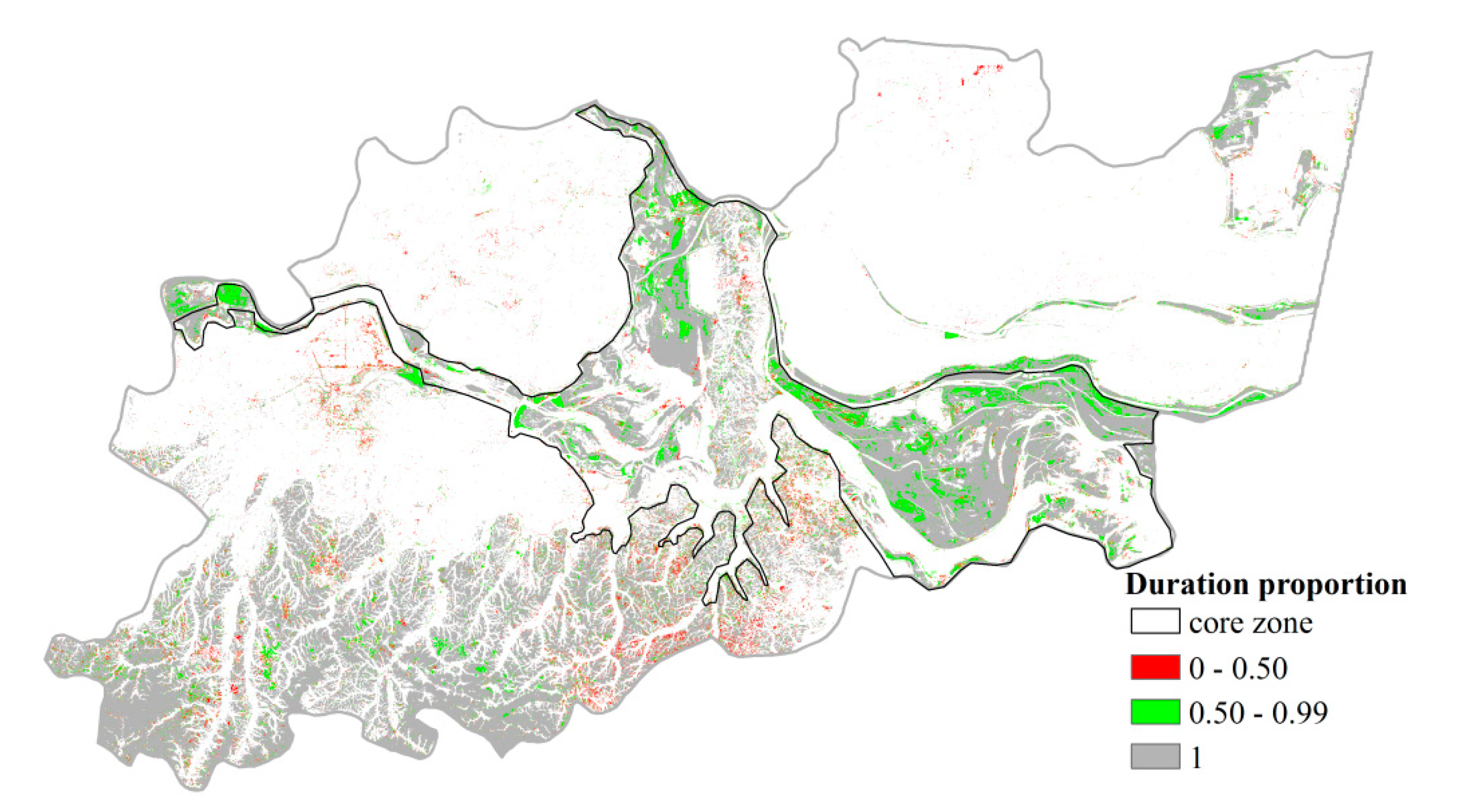
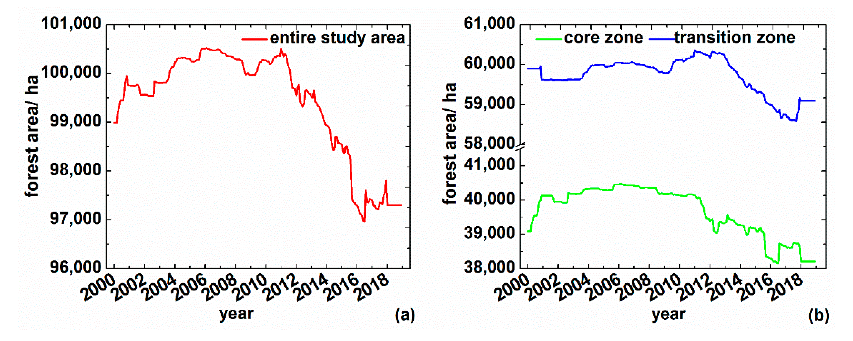
Although the proportion of forests in the core zone is lower than that in the transition zone, the proportion of changed forests in all the forests in the former is higher than that in the latter, especially in the areas with low elevation. The forests in the core zone are mainly distributed in the region with DEM ranging from 20 to 40 m, while over two-thirds of the forests in the transition zone were planted in the region with DEM exceeding 40 m (
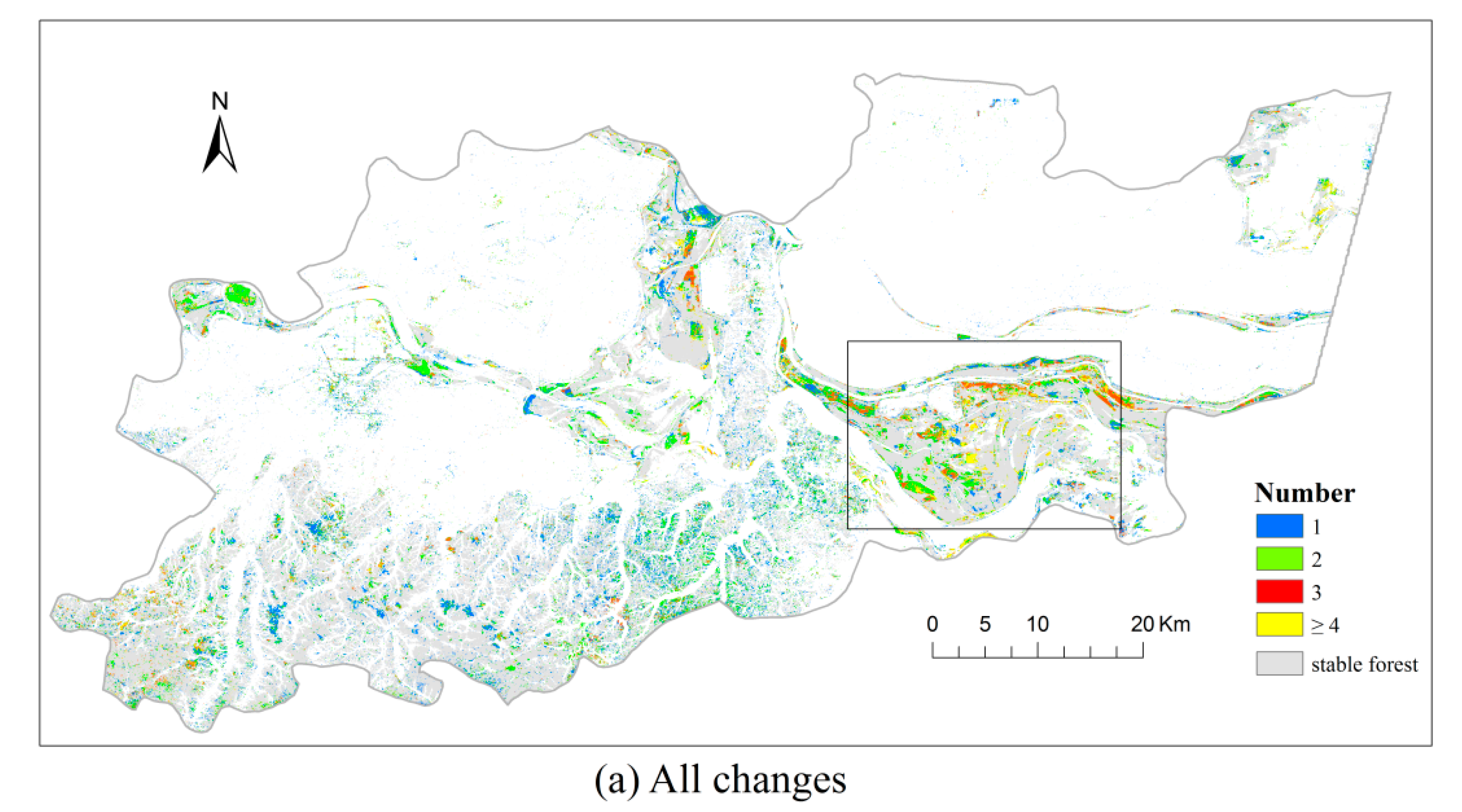
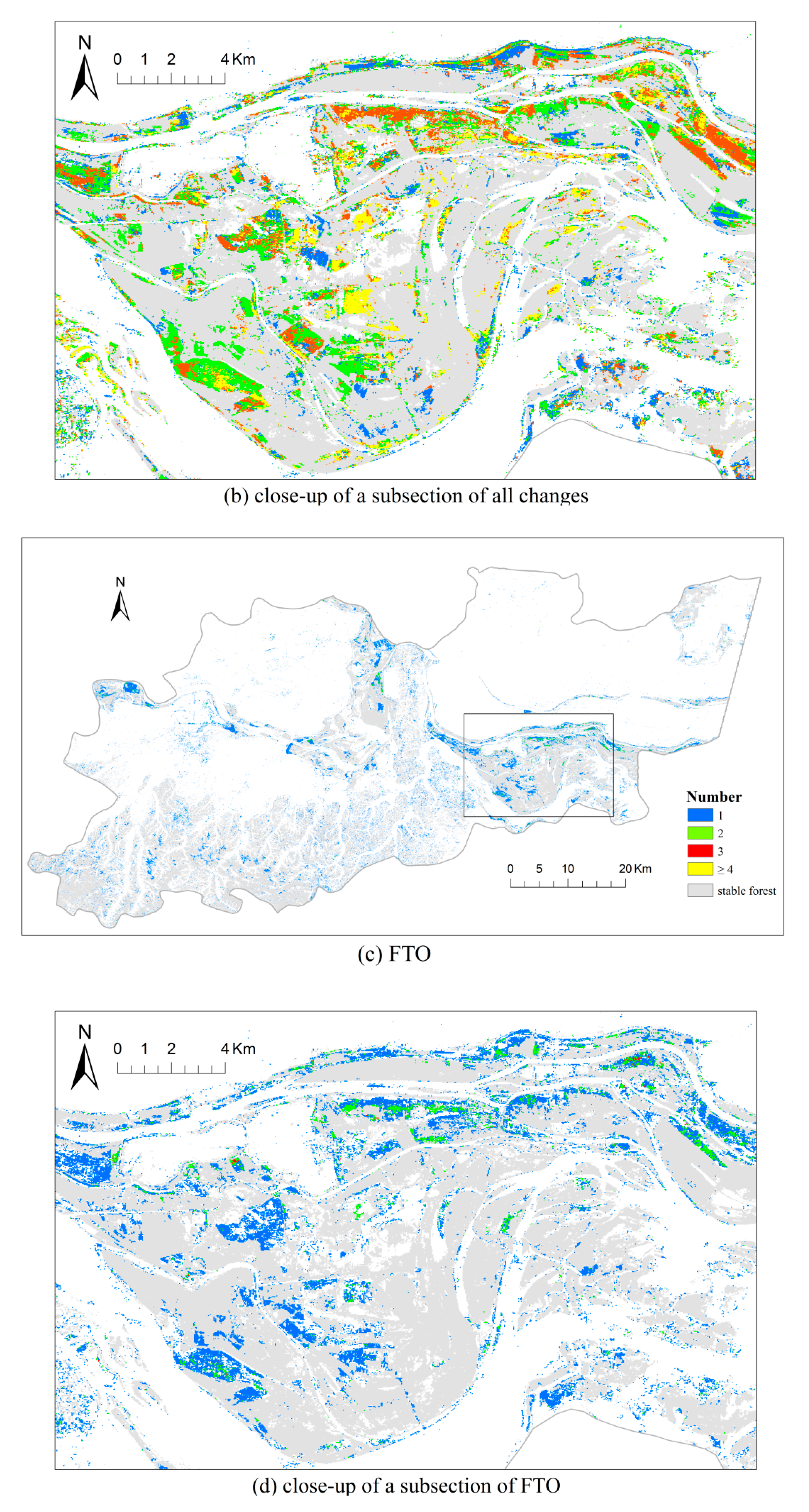
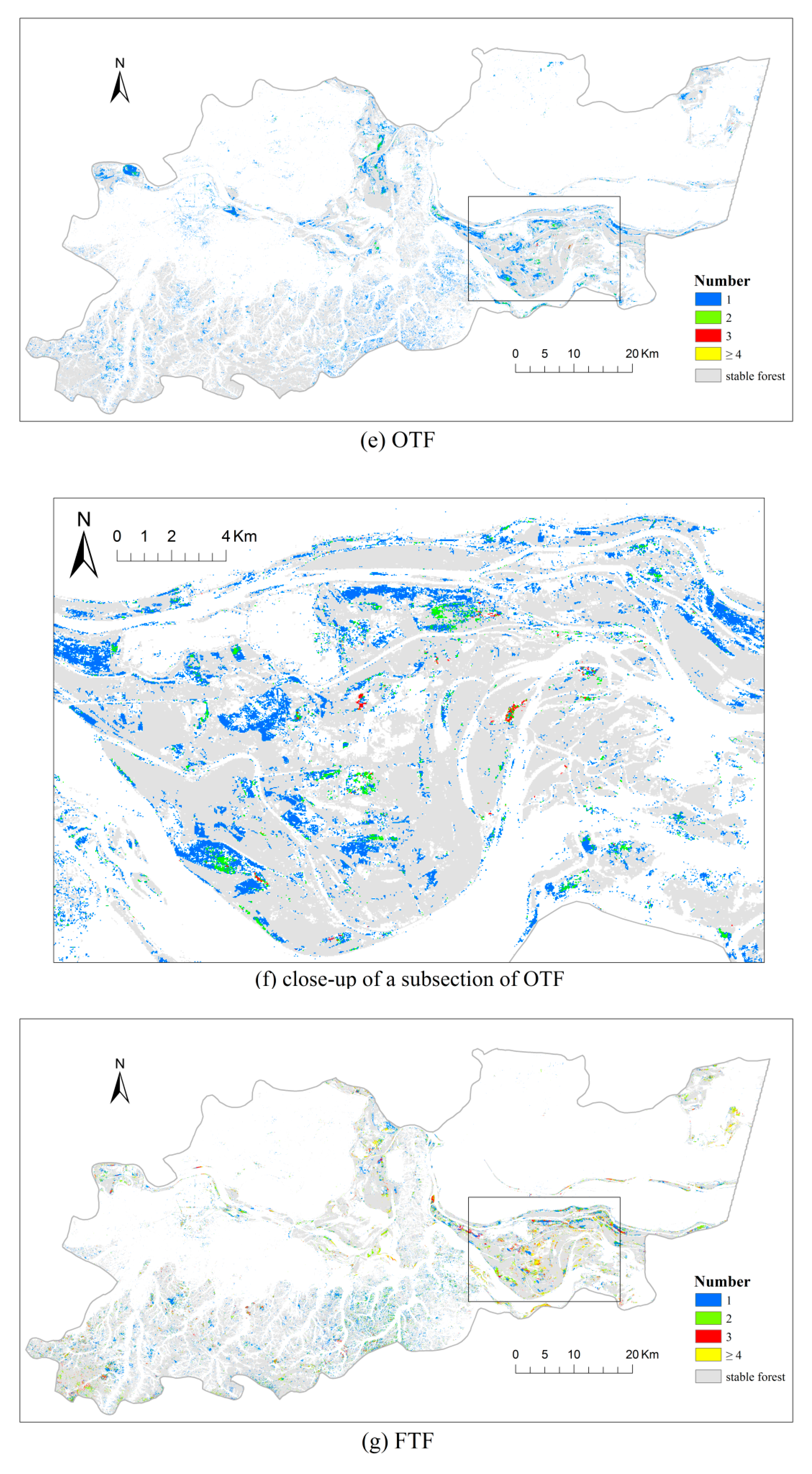
Table 8), and these forests are concentrated in the southwestern mountain with DEM over 50 m. Therefore, the forests with low elevation surrounding the water body in the core zone are easily flooded, which increases the number of FTF. In addition, the variation of timber price caused other land cover categories, such as cropland or shoal, to be switched to forest and replantation post-deforestation when prices rose, or the forest to be switched to other land cover when the price fell because of economic profit motivation, increasing the number of OTF or FTO. Meanwhile, the southwestern mountain with high elevation is suitable for tree plantation and unsuitable for growing crop and settlement, which leads to a relatively low proportion of OTF and FTO compared with the proportion of OTF and FTO in the core zone. These situations result in a high change frequency in the core zone.
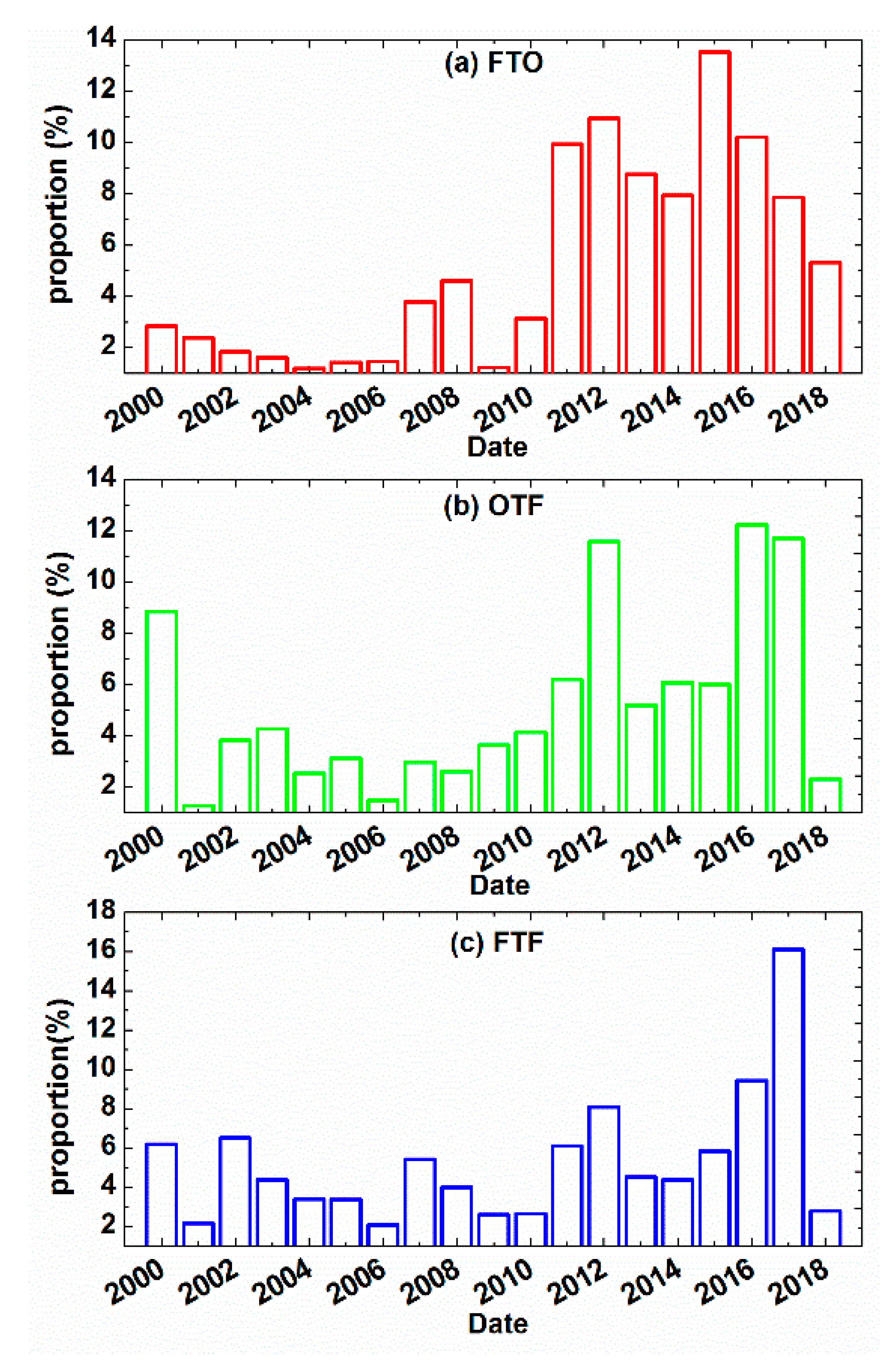
The low grain price and high timber price, policy incentives and market demand resulted in a rapid expansion of forest plantation in the West Dongting Lake region from 2000 to 2005. The early expansion mainly occurred in the core zone, and then in the transition zone since 2003. One potential factor is the transferal of parts of forest plantation from the core zone surrounding the water body to the transition zone due to TGD raising the water level of Dongting Lake. A possible reason for forest areas keeping relatively steady from 2006 to 2011 is a recovery in the grain price and stable timber price. Since 2011, a series of policies for protecting wetlands and restoring ecology made by the local government, especially the project of returning forest to wetland after 2013, forbade poplar plantation in the Dongting Lake region. It is the key driver of the difference of changes between before and after 2011. These policies have led to a continuing decline of the forest areas since 2011, except for the forest areas in the core zone sharply fluctuating with the fluctuating price of timber in 2014 and 2016. The policy of cleaning the poplar plantation in 2017 further accelerated the transferal of forest plantation from the core zone to the transition zone, resulting in a decline of forest areas in the core zone and an increasing trend in the transition zone during 2017. It also explained the high proportions of OTF and FTF in 2017 (Figure 10b,c). Therefore, the variation trend of forest areas indicated that anthropogenic factors, such as government policies and economic profits, are the dominating drivers of forest plantation in the West Dongting Lake region.
Results in this study effectively showed not only the final results of forest variations, but also the spatiotemporal dynamic process of forests and the potential drivers in West Dongting Lake, providing abundant knowledge for wetland ecosystem protection.

5. Conclusions

This study confirmed the applicability of the BFAST method to detect changes related to forest in the subtropical wetland ecosystem using the monthly Landsat NDVI time series and investigated the spatiotemporal variations of forest in the West Dongting Lake region between 2000 and 2018. By using the monthly Landsat time series generated by the spatiotemporal interpolator and data fusion algorithms, the forest changes, including FTO, OTF, and FTF, and land cover categories before and after breakpoints, could be effectively captured by integrating BFAST and RF algorithms, with an overall accuracy of 87.8%. The spatiotemporal variations of forest were described from the aspects of duration and distribution of forest, the number and timing of forest changes, and the variation of forest areas, respectively:
(1)
The forests are mainly distributed in the core zone surrounding the water body and the southwestern mountains. Over 60% of the stable forests are distributed in the transition zone, whereas the changed forests in the core zone and low elevation region are more prevalent.
(2)
Not only the proportion of pixels with FTF but also the number of FTF is higher than those of FTO and OTF. The forest change in the core zone is more frequent than that in the transition zone. Most changes occurred in the areas with DEM ranging from 20 to 40 m, in which the proportion of detected change number in the core zone is higher than that in the transition zone regardless of the change type.
(3)
Large parts of FTO occurred since 2011 due to the policy for protecting wetlands and restoring ecology. Some clear peaks of OTF were detected during 2000, 2012, 2016, and 2017 because of the jumping price of timber. FTF was relatively even for each year, except for one peak in 2017.
(4)
The variation of forest areas in the West Dongting Lake region experienced three steps: rapid expansion of forest plantation from 2000 to 2005, to which forest plantation in the core zone is the major contribution; relatively steady from 2006 to 2011, except for a small increase in the transition zone between 2008 and 2011; and continuous decline since 2011 with small sharp fluctuations in the core zone and a laggard downtrend in the transition zone. These variations were mainly caused by anthropogenic factors, such as the government policies and economic profits.

Author Contributions

Conceptualization, X.L., Z.L. and L.W.; Data Curation, L.W., L.Z. and B.X.; Formal Analysis, L.W. and Y.T.; Methodology, L.W., Y.T. and B.Z.; Supervision, Z.L. and X.L.; Validation, B.L. and Y.M.; Visualization, L.W. and L.Z.; Writing—Original Draft Preparation, L.W.; Writing—Review & Editing, Z.L., X.L. and M.L. All authors have read and agreed to the published version of the manuscript.

Funding

This work was supported by the programs of National Natural Science Foundation of China (Grant No. 41701387 and 41871223), and the Fundamental Research Funds for the Central Universities under Grant 2652017116.

Acknowledgments

We would like to thank USGS and NASA for providing Landsat and MODIS data. We want to thank Jan Verbesselt and Xiaolin Zhu for sharing the codes of BFAST, NSPI, and ESTARFM.

Conflicts of Interest

The authors declare no conflict of interest.

References

  1. Hu, W.; Zhao, J.; He, J.; Li, Y. Land use change and its landscape effect around Dongting Lake in recently 15 years. J. Cent. South Univ. For. Technol. 2017, 37, 91–97. [Google Scholar]
  2. Davidson, N.C. How much wetland has the world lost Long-term and recent trends in global wetland area. Mar. Freshw. Res. 2014, 65, 934–941. [Google Scholar] [CrossRef]
  3. Hu, S.; Niu, Z.; Chen, Y.; Li, L.; Zhang, H. Global wetlands Potential distribution, wetland loss, and status. Sci. Total Environ. 2017, 586, 319–327. [Google Scholar] [CrossRef] [PubMed]
  4. Li, Y.; Qin, H.; Xie, Y.; Wang, W.; Chen, X.; Zhang, C. Physiological mechanism for the reduction in soil water in poplar (Populus deltoides) plantations in Dongting Lake wetlands. Wetl. Ecol. Manag. 2014, 22, 25–33. [Google Scholar] [CrossRef] [Green Version]
  5. Hu, Y.; Huang, J.; Deng, F. Using remote sensing to monitor wetland cover change and succession in Dongting Lake of China during 1993–2010. In Proceedings of the 2011 International Conference on Multimedia Technology, ICMT 2011, Hangzhou, China, 26–28 July 2011; pp. 5668–5672. [Google Scholar]
  6. Jing, L.; Lyu, C.; Zhou, Y.; Zuo, A.; Lei, G. Spatio-temporal characteristics of the expansion of poplar plantation in West Dongting Lake wetland, China. Chin. J. Appl. Ecol. 2016, 27, 2039–2047. [Google Scholar]
  7. Liu, Y.; Shi, L.; Duo, H.; Peng, B.; Lü, C.; Zhu, Y.; Lei, G. Disturbance-driven changes to landscape patterns and responses of waterbirds at West Dongting Lake, China. Biodivers. Sci. 2013, 21, 666–676. [Google Scholar]
  8. Li, Y.; Chen, X.; Xie, Y.; Li, X.; Li, F.; Hou, Z. Effects of young poplar plantations on understory plant diversity in the Dongting Lake wetlands, China. Sci. Rep. 2014, 4, 1–8. [Google Scholar] [CrossRef]
  9. Bruzzone, L.; Cossu, R.; Vernazza, G. Detection of land-cover transitions by combining multidate classifiers. Pattern Recognit. Lett. 2004, 25, 1491–1500. [Google Scholar] [CrossRef]
  10. Chen, J.; Chen, X.; Cui, X.; Chen, J. Change vector analysis in posterior probability space A new method for land cover change detection. IEEE Geosci. Remote Sens. Lett. 2011, 8, 317–321. [Google Scholar] [CrossRef]
  11. Lu, D.; Mausel, P.; Brondízio, E.; Moran, E. Change detection techniques. Int. J. Remote Sens. 2004, 25, 2365–2407. [Google Scholar] [CrossRef]
  12. Verbesselt, J.; Hyndman, R.; Newnham, G.; Culvenor, D. Detecting trend and seasonal changes in satellite image time series. Remote Sens. Environ. 2010, 114, 106–115. [Google Scholar] [CrossRef]
  13. Zhang, L.; Wu, C. Advance and Future development of change detection for multi-temporal remote sensing imagery. Acta Geod. Cartogr. Sin. 2017, 46, 1447–1459. [Google Scholar]
  14. Zhao, Z.; Meng, Y.; Yue, A.; Huang, Q.; Kong, Y.; Yuan, Y.; Liu, X.; Lin, L.; Zhang, M. Review of remotely sensed time series data for change detection. J. Remote Sens. 2016, 20, 1110–1125. [Google Scholar]
  15. Huang, C.; Goward, S.N.; Masek, J.G.; Thomas, N.; Zhu, Z.; Vogelmann, J.E. An automated approach for reconstructing recent forest disturbance history using dense Landsat time series stacks. Remote Sens. Environ. 2010, 114, 183–198. [Google Scholar] [CrossRef]
  16. Kennedy, R.E.; Yang, Z.; Cohen, W.B. Detecting trends in forest disturbance and recovery using yearly landsat time series: 1. LandTrendr-temporal segmentation algorithms. Remote Sens. Environ. 2010, 114, 2897–2910. [Google Scholar] [CrossRef]
  17. Griffiths, P.; Kuemmerle, T.; Kennedy, R.E.; Abrudan, I.V.; Knorn, J.; Hostert, P. Using annual time-series of Landsat images to assess the effects of forest restitution in post-socialist Romania. Remote Sens. Environ. 2012, 118, 199–214. [Google Scholar] [CrossRef]
  18. Kennedy, R.E.; Yang, Z.; Braaten, J.; Copass, C.; Antonova, N.; Jordan, C. Attribution of disturbance change agent from Landsat time-series in support of habitat monitoring in the Puget Sound region, USA. Remote Sens. Environ. 2015, 166, 271–285. [Google Scholar] [CrossRef]
  19. Wu, D.; Li, B.; Yang, A. Estimation of tree height and biomass based on long time series data of landsat. Eng. Sur. Map. 2017, 26, 1–5. [Google Scholar]
  20. Cai, S.; Liu, D. Detecting change dates from dense satellite time series using a sub-annual change detection algorithm. Remote Sens. 2015, 7, 8705–8727. [Google Scholar] [CrossRef] [Green Version]
  21. Zhu, Z.; Woodcock, C.E. Continuous change detection and classification of land cover using all available Landsat data. Remote Sens. Environ. 2014, 144, 152–171. [Google Scholar] [CrossRef] [Green Version]
  22. Boriah, S. Time Series Change Detection: Algorithms for Land Cover Change. Ph.D. Thesis, University of Minnesota, Minneapolis, MN, USA, January 2010. [Google Scholar]
  23. Verbesselt, J.; Hyndman, R.; Zeileis, A.; Culvenor, D. Phenological change detection while accounting for abrupt and gradual trends in satellite image time series. Remote Sens. Environ. 2010, 114, 2970–2980. [Google Scholar] [CrossRef] [Green Version]
  24. Chen, L.; Michishita, R.; Xu, B. Abrupt spatiotemporal land and water changes and their potential drivers in Poyang Lake, 2000–2012. ISPRS J. Photogramm. Remote Sens. 2014, 98, 85–93. [Google Scholar] [CrossRef]
  25. Platt, R.V.; Ogra, M.V.; Badola, R.; Hussain, S.A. Conservation-induced resettlement as a driver of land cover change in India an object-based trend analysis. Appl. Geogr. 2016, 69, 75–86. [Google Scholar] [CrossRef]
  26. Tsutsumida, N.; Saizen, I.; Matsuoka, M.; Ishii, R. Land Cover Change Detection in Ulaanbaatar Using the Breaks for Additive Seasonal and Trend Method. Land 2013, 2, 534–549. [Google Scholar] [CrossRef]
  27. Dutrieux, L.P.; Verbesselt, J.; Kooistra, L.; Herold, M. Monitoring forest cover loss using multiple data streams, a case study of a tropical dry forest in Bolivia. ISPRS J. Photogramm. Remote Sens. 2015, 107, 112–125. [Google Scholar] [CrossRef]
  28. Fang, X.; Zhu, Q.; Ren, L.; Chen, H.; Wang, K.; Peng, C. Large-scale detection of vegetation dynamics and their potential drivers using MODIS images and BFAST: A case study in Quebec, Canada. Remote Sens. Environ. 2018, 206, 391–402. [Google Scholar] [CrossRef]
  29. Verbesselt, J.; Zeileis, A.; Herold, M. Near real-time disturbance detection using satellite image time series. Remote Sens. Environ. 2012, 123, 98–108. [Google Scholar] [CrossRef]
  30. Saxena, R.; Watson, L.T.; Wynne, R.H.; Brooks, E.B.; Thomas, V.A.; Yang, Z.; Kennedy, R.E. Towards a polyalgorithm for land use change detection. ISPRS J. Photogramm. Remote Sens. 2018, 144, 217–234. [Google Scholar] [CrossRef]
  31. Waller, E.K.; Villarreal, M.L.; Poitras, T.B.; Nauman, T.W.; Duniway, M.C. Landsat time series analysis of fractional plant cover changes on abandoned energy development sites. Int. J. Appl. Earth Obs. Geoinf. 2018, 73, 407–419. [Google Scholar] [CrossRef]
  32. Yuan, Y.; Meng, Y.; Lin, L.; Sahli, H.; Yue, A.; Chen, J.; Zhao, Z.; Kong, Y.; He, D. Continuous Change Detection and Classification Using Hidden Markov Model: A Case Study for Monitoring Urban Encroachment onto Farmland in Beijing. Remote Sens. 2015, 7, 15318–15339. [Google Scholar] [CrossRef] [Green Version]
  33. Chen, J.; Chen, J.; Liu, H.; Peng, S. Detection of cropland change using multi-harmonic based phenological trajectory similarity. Remote Sens. 2018, 10, 1020. [Google Scholar] [CrossRef] [Green Version]
  34. Jin, S.; Sader, S.A. MODIS time-series imagery for forest disturbance detection and quantification of patch size effects. Remote Sens. Environ. 2005, 99, 462–470. [Google Scholar] [CrossRef]
  35. Hansen, M.C.; Potapov, P.V.; Moore, R.; Hancher, M.; Turubanova, S.A.; Tyukavina, A.; Thau, D.; Stehman, S.V.; Goetz, S.J.; Loveland, T.R.; et al. High-resolution global maps of 21st-century forest cover change. Science 2013, 342, 850–853. [Google Scholar] [CrossRef] [PubMed] [Green Version]
  36. Townshend, J.R.; Masek, J.G.; Huang, C.; Vermote, E.F.; Gao, F.; Channan, S.; Sexton, J.O.; Feng, M.; Narasimhan, R.; Kim, D.; et al. Global characterization and monitoring of forest cover using Landsat data opportunities and challenges. Int. J. Digit. Earth 2013, 5, 373–397. [Google Scholar] [CrossRef] [Green Version]
  37. Loveland, T.R.; Irons, J.R. Landsat 8: The plans, the reality, and the legacy. Remote Sens. Environ. 2016, 185, 1–6. [Google Scholar] [CrossRef] [Green Version]
  38. Wulder, M.A.; White, J.C.; Loveland, T.R.; Woodcock, C.E.; Belward, A.S.; Cohen, W.B.; Fosnight, E.A.; Shaw, J.; Masek, J.G.; Roy, D.P. The global Landsat archive Status, consolidation, and direction. Remote Sens. Environ. 2016, 185, 271–283. [Google Scholar] [CrossRef] [Green Version]
  39. Vogelmann, J.E.; Gallant, A.L.; Shi, H.; Zhu, Z. Perspectives on monitoring gradual change across the continuity of Landsat sensors using time-series data. Remote Sens. Environ. 2016, 185, 258–270. [Google Scholar] [CrossRef] [Green Version]
  40. Chen, J.; Zhu, X.; Vogelmann, J.E.; Gao, F.; Jin, S. A simple and effective method for filling gaps in Landsat ETM+ SLC-off images. Remote Sens. Environ. 2011, 115, 1053–1064. [Google Scholar] [CrossRef]
  41. Zhu, X.; Gao, F.; Liu, D.; Chen, J. A modified neighborhood similar pixel interpolator approach for removing thick clouds in landsat images. IEEE Geosci. Remote Sens. Lett. 2012, 9, 521–525. [Google Scholar] [CrossRef]
  42. Zhu, X.; Helmer, E.H.; Chen, J.; Liu, D. An Automatic System for Reconstructing High-Quality Seasonal Landsat Time Series. In Remote Sensing Time Series Image Processing; Taylor and Francis Series in Imaging Science; Weng, Q., Ed.; CRC Press: Boca Raton, FL, USA, 2018; pp. 25–42. [Google Scholar]
  43. Zhu, X.; Chen, J.; Gao, F.; Chen, X.; Masek, J.G. An enhanced spatial and temporal adaptive reflectance fusion model for complex heterogeneous regions. Remote Sens. Environ. 2010, 114, 2610–2623. [Google Scholar] [CrossRef]
  44. Liu, M.; Liu, X.; Wu, L.; Zou, X.; Jiang, T.; Zhao, B. A Modified spatiotemporal fusion algorithm using phenological information for predicting reflectance of paddy rice in southern China. Remote Sens. 2018, 10, 772. [Google Scholar] [CrossRef] [Green Version]
  45. The United States Geological Service (USGS) LSDS Science Research and Development (LSRD). Available online: https://espa.cr.usgs.gov (accessed on 10 January 2020).
  46. National Aeronautics and Space Administration (NASA) Level-1 and Atmosphere Archive & Distribution System Distributed Active Archive Center (LAADSDAAC). Available online: https://ladsweb.modaps.eosdis.nasa.gov (accessed on 10 January 2020).
  47. National Aeronautics and Space Administration (NASA) Land Processes Distributed Active Archive Center (LPDAAC). Available online: https://lpdaac.usgs.gov/ (accessed on 10 January 2020).
  48. Cleveland, R.B.; Cleveland, W.S.; McRae, J.E. STL: A seasonal trend decomposition procedure based on loess. J. Off. Statist. 1990, 6, 3–73. [Google Scholar]
  49. Chu, C.S.J.; Hornik, K.; Kaun, C.M. MOSUM tests for parameter constancy. Br. J. Psychiatry 1995, 112, 211–212. [Google Scholar] [CrossRef]
  50. Schwarz, G. Estimating the dimension of a model. Ann. Stat. 1978, 14, 590–606. [Google Scholar] [CrossRef]
  51. Venables, W.N.; Ripley, B.D. Modern Applied Statistics with S-PLUS.; Springer: Berlin/Heidelberg, Germany, 2002; pp. 156–163. [Google Scholar]
  52. Breiman, L. Random Forests. Mach. Learn. 2001, 45, 5–32. [Google Scholar] [CrossRef] [Green Version]
  53. Gómez, C.; White, J.C.; Wulder, M.A. Optical remotely sensed time series data for land cover classification: A review. ISPRS J. Photogramm. Remote Sens. 2016, 116, 55–72. [Google Scholar] [CrossRef] [Green Version]
  54. Cohen, W.B.; Yang, Z.; Kennedy, R. Detecting trends in forest disturbance and recovery using yearly Landsat time series: 2. TimeSync—Tools for calibration and validation. Remote Sens. Environ. 2010, 114, 2911–2924. [Google Scholar] [CrossRef]
  55. Grogan, K.; Pflugmacher, D.; Hostert, P.; Kennedy, R.; Fensholt, R. Cross-border forest disturbance and the role of natural rubber in main-land Southeast Asia using annual Landsat time series. Remote Sens. Environ. 2015, 169, 438–453. [Google Scholar] [CrossRef]
  56. Jin, S.; Yang, L.; Danielson, P.; Homer, C.; Fry, J.; Xian, G. A comprehensive change detection method for updating the national land cover database to circa 2011. Remote Sens. Environ. 2013, 132, 159–175. [Google Scholar] [CrossRef] [Green Version]
  57. DeVries, B.; Verbesselt, J.; Kooistra, L.; Herold, M. Robust monitoring of small-scale forest disturbances in a tropical montane forest using Landsat time series. Remote Sens. Environ. 2015, 161, 107–121. [Google Scholar] [CrossRef]
  58. Zhu, Z. Change detection using landsat time series: A review of frequencies, preprocessing, algorithms, and applications. ISPRS J. Photogramm. Remote Sens. 2017, 130, 370–384. [Google Scholar] [CrossRef]
  59. Hamunyela, E.; Verbesselt, J.; Herold, M. Using spatial context to improve early detection of deforestation from Landsat time series. Remote Sens. Environ. 2016, 172, 126–138. [Google Scholar] [CrossRef]
  60. Hermosilla, T.; Wulder, M.A.; White, J.C.; Coops, N.C.; Hobart, G.W. Regional detection, characterization, and attribution of annual forest change from 1984 to 2012 using Landsat-derived time-series metrics. Remote Sens. Environ. 2015, 170, 121–132. [Google Scholar] [CrossRef]
  61. Behling, R.; Milewski, R.; Chabrillat, S. Spatiotemporal shoreline dynamics of Namibian coastal lagoons derived by a dense remote sensing time series approach. Int. J. Appl. Earth Obs. Geoinf. 2018, 68, 262–271. [Google Scholar] [CrossRef] [Green Version]
  62. Guttler, F.; Ienco, D.; Nin, J.; Teisseire, M.; Poncelet, P. A graph-based approach to detect spatiotemporal dynamics in satellite image time series. ISPRS J. Photogramm. Remote Sens. 2017, 130, 92–107. [Google Scholar] [CrossRef] [Green Version]
  63. De Beurs, K.M.; Henebry, G.M. A statistical framework for the analysis of long image time series. Int. J. Remote Sens. 2005, 26, 1551–1573. [Google Scholar] [CrossRef]
  64. Lu, M.; Pebesma, E.; Sanchez, A.; Verbesselt, J. Spatio-temporal change detection from multidimensional arrays Detecting deforestation from MODIS time series. ISPRS J. Photogramm. Remote Sens. 2016, 117, 227–236. [Google Scholar] [CrossRef]
  65. Coulibaly, S.; Kamsu-Foguem, B.; Kamissoko, D.; Traore, D. Deep neural networks with transfer learning in millet crop images. Comput. Ind. 2019, 108, 115–120. [Google Scholar] [CrossRef] [Green Version]
  66. Pan, X.; Zhao, J. A central-point-enhanced convolutional neural network for high-resolution remote-sensing image classification. Int. J. Remote Sens. 2017, 38, 6554–6581. [Google Scholar] [CrossRef]
  67. Zhao, S.; Liu, X.; Ding, C.; Liu, S.; Wu, C.; Wu, L. Mapping Rice Paddies in Complex Landscapes with Convolutional Neural Networks and Phenological Metrics. GISci. Remote Sens. 2019. [Google Scholar] [CrossRef]
  68. Jiang, T.; Liu, X.; Wu, L. Method for Mapping Rice Fields in Complex Landscape Areas Based on Pre-Trained Convolutional Neural Network from HJ-1 A/B Data. ISPRS Int. Geo-Inf. 2018, 7, 418. [Google Scholar] [CrossRef] [Green Version]
  69. Wang, L.; Liu, M.; Liu, X.; Wu, L.; Wang, P.; Wu, C. Hierarchical classification method for mapping rice-cropping systems using pretrained convolutional neural network with spatial and spectral trajectories of Sentinel-2 time series. J. Appl. Remote Sens. 2020, 14, 014506. [Google Scholar] [CrossRef]
  70. Google Earth Engine (GEE) Platform. Available online: https://earthengine.google.org/ (accessed on 10 January 2020).
  71. Dong, J.; Xiao, X.; Menarguez, M.A.; Zhang, G.; Qin, Y.; Thau, D. Mapping paddy rice planting area in northeastern Asia with Landsat 8 images, phenology-based algorithm and Google Earth Engine. Remote Sens. Environ. 2016, 185, 142–154. [Google Scholar] [CrossRef] [PubMed] [Green Version]
  72. Zhu, L.; Liu, X.; Wu, L.; Tang, Y.; Meng, Y. Long-Term Monitoring of Cropland Change near Dongting Lake, China, Using the LandTrendr Algorithm with Landsat Imagery. Remote Sens. 2019, 11, 1234. [Google Scholar] [CrossRef] [Green Version]
Figure 1. Geographic location, Landsat and DEM image of the study area: (a) general location within China, (b) within Hunan Province, and (c) within the Dongting Lake region; (d) Landsat 8 OLI image (RGB = near-infrared, red, and green band); and (e) Global Digital Elevation Model (GDEM) image of the study area.
Remotesensing 12 00341 g001aRemotesensing 12 00341 g001b
Figure 2. Flowchart of investigating the spatiotemporal variations of forest in the West Dongting Lake region. NSPI, MNSPI and ESTARFM represent the spatiotemporal interpolation method named Neighborhood Similar Pixel Interpolator and its modified version, and a spatiotemporal data fusion algorithm named enhanced spatial and temporal adaptive reflectance fusion model, respectively. BFAST is the change detection algorithm named Breaks For Additive Seasonal and Trend, and RF represents random forest algorithm.
Remotesensing 12 00341 g002
Figure 3. Proportions of 197 available Landsat images with different percentages of contaminated pixels between 2000 and 2018 in the West Donting Lake region.
Remotesensing 12 00341 g003
Figure 4. Detected changes in the seasonal and trend component of monthly NDVI time series between 2000 and 2018 by using BFAST: (a) The breakpoint in the seasonal component St represents the conversion from forest to other land cover categories (FTO); (b) the breakpoint in the seasonal component St represents the conversion from other land cover categories to forest (OTF), and two breakpoints in the trend component Tt represent flooding and recovery (FTF); (c) two breakpoints closely adjacent to each other in the trend component Tt represent replantation post-deforestation (FTF). Yt represents the original observed data, and et represents the remainder component. The dash line represents the breakpoint and indicates when abrupt change occurred. The confidence intervals of the estimated date of abrupt changes are shown (red).
Remotesensing 12 00341 g004
Figure 5. Examples of accuracy assessment for the detected changes and corresponding Landsat images (RGB = near-infrared, red, and green band) before and after abrupt changes: (a) Forest to other land cover (urban), (b) Other land cover (shoal) to Forest, (c) Flooding, and (d) Replantation post-deforestation. Yt is the original observed data; Tt, St, and et separately represent the trend, seasonal, and remainder component decomposed by BFAST. The dashed line represents the breakpoint and indicates when abrupt change occurred. The confidence intervals of the estimated date of abrupt changes are shown (red).
Remotesensing 12 00341 g005aRemotesensing 12 00341 g005b
Figure 6. Distribution map of the duration proportion (Df) of forest plantation between 2000 and 2018. Df is calculated as the ratio of the number of time phases when the land cover category within the pixel is forest to the total number of time phases (or images) within the monthly Landsat time series.
Remotesensing 12 00341 g006
Figure 7. Spatial distribution of the number (iK) of abrupt changes between 2000 and 2018 for different forest change types and their close-up subsection: (a,b) all changes; (c,d) conversion from forest to other land cover categories (FTO); (e,f) conversion from other land cover categories to forest (OTF); and (g,h) conversion from forest to forest (FTF, such as flooding and replantation post-deforestation).
Remotesensing 12 00341 g007aRemotesensing 12 00341 g007bRemotesensing 12 00341 g007cRemotesensing 12 00341 g007d
Figure 8. Proportion (ML) of the number of different forest change types for each DEM range and region: (a) all changes; (b) conversion from forest to other land cover categories (FTO); (c) conversion from other land cover categories to forest (OTF); and (d) conversion from forest to forest (FTF, such as flooding and replantation post-deforestation). ML is calculated as the ratio of the number of abrupt changes in a certain region or DEM range to the total number of abrupt changes in the whole study area between 2000 and 2018 for each change type.
Remotesensing 12 00341 g008
Figure 9. Spatial distribution of the timing (Tl) of last change of different forest change types and their close up of the subsection detected from monthly NDVI time-series: (a,b) conversion from forest to other land cover categories (FTO), (c,d) conversion from other land cover categories to forest (OTF), and (e,f) conversion from forest to forest (FTF, such as flooding and replantation post-deforestation). The changed forest pixels with nonFTO (or nonOTF, or nonFTF) represent that no FTO (or OTF, FTF) occurred in these changed pixels.
Remotesensing 12 00341 g009aRemotesensing 12 00341 g009bRemotesensing 12 00341 g009c
Figure 10. Annual proportion (APK,T) of different forest change types detected from Landsat NDVI time series between 2000 and 2018: (a) conversion from forest to other land cover categories (FTO), (b) conversion from other land cover categories to forest (OTF), and (c) conversion from forest to forest (FTF, such as flooding and replantation post-deforestation). APK,T is calculated as the ratio of the number of changes in a certain year to the total number of changes between 2000 and 2018 for each change type.
Remotesensing 12 00341 g010
Figure 11. Variation of forest areas (AL,t) between 2000 and 2018 for (a) entire study area and (b) core and transition zones.
Remotesensing 12 00341 g011
Table 1. Number of available and missing images for generating a monthly Landsat time series between 2000 and 2018.
YearNumber of Available ImagesNumber of Missing Images
200094
2001112
2002102
200357
2004151
2005103
200693
200785
2008121
2009133
2010103
2011115
201276
2013112
2014104
2015103
2016122
2017123
2018120
total19759
Table 2. Datasets used in this study.
DataDescriptionSource
Landsat 5, 7 and 8All 197 available Landsat images (Table 1) used as inputs to NSPI and MNSPI for SLC-off gaps filling and cloud removal. One-hundred-and-sixty-nine out of 197 images and 59 prediction images reconstructed with ESTARFM, a total of 228 images, utilized to generate a monthly Landsat time series for change detection with BFAST. (1) The United States Geological Service (USGS) [45]; (2) prediction images reconstructed with ESTARFM.
MODISSeventy-three MODIS surface reflectance 8-day composite images used as inputs to ESTARFM for reconstructing the 59 missing Landsat images.National Aeronautics and Space Administration (NASA) Level-1 and Atmosphere Archive & Distribution System Distributed Active Archive Center (LAADSDAAC) [46].
High-resolution imagesImages for validation of change detection and land cover classification, and determination of land cover category of each reference pixel with Landsat images together.Google earth
GDEMASTER GDEM version 2.0 data with 1 arc-second grid used for analyzing spatiotemporal dynamics of forest.NASA Land Processes Distributed Active Archive Center (LPDAAC) [47].
Table 3. Land cover reference data collected at four dates for classification.
ClassDateTotal
2002-09-022007-08-072013-08-072017-08-18
Crop10661397106618965425
Forest10911204109115054891
Shoal161126188190665
Urban295929572959152110,396
Water10801008108015924760
Total635766926384670426,137
Table 4. Indicators for describing spatiotemporal dynamics of forest.
CategoryIndicatorFormulaMeaning/Explanation
DurationThe duration proportion Df of forest plantation in each pixel D f = T P f 228 TPf represents the number of time phases when the land cover category within the pixel is forest; 228 is the total number of time phases (or images) within the monthly Landsat time series
Proportion of stable (Ps) and changed forests (Pc) P c = N c N f
P s = N s N f
Nc and Ns represent the number of changed and stable forest pixels, respectively
Nf represents the number of forest pixels
NumberNumber iK of abrupt changes [24] i K = 1 ,   2 , , n
K = A L L ,   F T O ,   O T F ,   F T F
K represents the change type
Number Nc(i) and proportion Pc(i) of changed pixels with i times abrupt changes P c ( i ) = N c ( i ) N f
N c = i = 1 n N c   ( i )
Proportion ML of abrupt changes in region L M L = i = 1 n i × N c ( i , L ) i = 1 n i × N c ( i ) N c ( i , L ) represents the number of changed pixels with i times abrupt changes in region L
i = 1 n i × N c ( i )   represents the total number of abrupt changes
The ratio RL of the number of abrupt changes to the number of changed pixels in region L R L = i = 1 n i × N c ( i , L ) N c ( L ) N c ( L ) represents the number of change pixels in region L
TimingTiming (Tl) of last change [25] T l = 2000 ,   2001 , , 2018
Annual proportion APK,T of abrupt changes [24] A P K , T = i = 1 n i × N c ( i , T , K ) i = 1 n i × N c ( i )
T = 2000 ,   2001 , , 2018
The ratio of the number of changes in a certain year to the total number of changes.
N c ( i , T , K ) represents the number of changed pixels with i times change type K in T
Areasforest areas AL,t in region L in t A L , t =   n f ( L , t ) × s
t = 1 ,   2 , , 228
n f ( L , t ) represents the number of forest pixels in region L in t. s is the area of one Landsat pixel (900 m2)
Table 5. Accuracy assessment of change detection.
Changed PixelsStable PixelsTotalUser’s Accuracy
Changed pixels2534730084.3%
Stable pixels2627430091.3%
Total279321
Producer’s accuracy90.7%85.4%Overall87.8%
Table 6. Accuracy assessment of the timing of change detection.
Same timeLate ≤ 2 monthsLate > 2 monthsTotal
Changed pixels1963324253
proportion77.47%13.04%9.49%100%
Table 7. Accuracy assessment of classification with the RF algorithm.
Overall Accuracy = 7285/7837 = 92.96% Kappa Coefficient = 0.9026
Ground Truth (Pixels)
ClassCropForestShoalUrbanWaterUser Accuracy
crop1500480353892.54%
forest20133845221592.92%
shoal0101410192.76%
urban109422304911391.98%
water187423125796.03%
Total1647144519231291424
Producer accuracy91.07%92.60%73.44%97.44%88.27%
Table 8. Proportion (%) of stable (PS) and changed (Pc) forests for each DEM range and region.
LocationType DEM (m)Total
≤2020–3030–4040–50≥50
Core zoneChanged forest0.123.896.460.810.411.69
Stable forest0.2010.0414.242.021.1327.63
Transition zoneChanged forest0.082.754.661.866.8816.23
Stable forest0.073.688.15527.5544.45
totalChanged forest0.206.6411.122.677.2827.92
Stable forest0.2713.7222.397.0228.6872.08
proportion of changed forest42.5532.6133.1827.5520.24
Table 9. Number (Nc(i)) and proportion (Pc(i)) of pixels with single (or multiple) occurrence(s) of abrupt change between 2000 and 2018.
Number of Abrupt ChangesAllFTOOTFFTF
NumberProportion (%)NumberProportion (%)NumberProportion (%)NumberProportion (%)
0851,17272.081,023,09586.641,040,50588.11995,48584.30
1125,27710.61145,75412.34129,87611.0091,5307.75
2122,40410.3711,6650.9998970.8456,1964.76
351,6494.373750.036090.0521,9621.86
≥430,3912.5740.0060.0015,7201.33
TCP 1329,72127.92157,79813.36140,38811.89185,40815.70
TNB 2665,744 170,225 151,521 343,998
1 TCP represents Total of changed pixels, and 2 TNB represents Total number of breakpoints.

