On the Capabilities of the Italian Airborne FMCW AXIS InSAR System
by
 , and
, and
Carmen Esposito
1 ,
,
Antonio Natale
1,*,
Gianfranco Palmese
2,
Paolo Berardino
1,
Riccardo Lanari
1 and
Stefano Perna
1,3
1
Institute for Remote Sensing of Environment (IREA), National Research Council (CNR), 80124 Napoli, Italy
2
Elettra Microwave, 80143 Napoli, Italy
3
Department of Engineering (DI), Università degli Studi di Napoli “Parthenope”, 80143 Napoli, Italy
*
Author to whom correspondence should be addressed.
Remote Sens. 2020, 12(3), 539; https://0-doi-org.brum.beds.ac.uk/10.3390/rs12030539
Submission received: 31 December 2019
/
Revised: 25 January 2020
/
Accepted: 4 February 2020
/
Published: 6 February 2020
(This article belongs to the Special Issue Radar Imaging in Challenging Scenarios from Smart and Flexible Platforms)
Abstract
:Airborne Synthetic Aperture Radar (SAR) systems are gaining increasing interest within the remote sensing community due to their operational flexibility and observation capabilities. Among these systems, those exploiting the Frequency-Modulated Continuous-Wave (FMCW) technology are compact, lightweight, and comparatively low cost. For these reasons, they are becoming very attractive, since they can be easily mounted onboard ever-smaller and highly flexible aerial platforms, like helicopters or unmanned aerial vehicles (UAVs). In this work, we present the imaging and topographic capabilities of a novel Italian airborne SAR system developed in the frame of cooperation between a public research institute (IREA-CNR) and a private company (Elettra Microwave S.r.l.). The system, which is named AXIS (standing for Airborne X-band Interferometric SAR), is based on FMCW technology and is equipped with a single-pass interferometric layout. In the work we first provide a description of the AXIS system. Then, we describe the acquisition campaign carried out in April 2018, just after the system completion. Finally, we perform an analysis of the radar data acquired during the campaign, by presenting a quantitative assessment of the quality of the SLC (Single Look Complex) SAR images and the interferometric products achievable through the system. The overall analysis aims at providing first reference values for future research and operational activities that will be conducted with this sensor.
1. Introduction
Synthetic Aperture Radar (SAR) systems are microwave remote sensors that are mounted on board moving platforms in order to obtain high spatial resolution in the along-track direction by emulating the acquisition mechanism of large-aperture antennas [1,2]. Very common platforms used to mount SAR systems are satellites [1,2,3,4,5,6] (spaceborne systems), airplanes [7,8,9,10], helicopters [11], and, more recently, drones [12,13] (aerial systems). Due to their peculiarities, spaceborne and aerial SAR systems are, to some extent, complementary.
Spaceborne systems guarantee very wide spatial coverage. However, they are forced to follow polar orbits, thus flying practically only along the South–North (or North–South) direction. This poses some limitations to the full exploitation of those techniques, such as Differential SAR Interferometry (DInSAR) or Along Track Interferometry (ATI), which allow us to measure only the Line of Sight (LoS) component of the remotely sensed phenomenon. Moreover, with the currently operative spaceborne SAR constellations [3,4], the revisiting time, that is, the time interval elapsing between subsequent observations of the same area, is on the order of several days. This makes it impossible on the one hand to illuminate the area of interest in a timely way in case of emergencies, and on the other hand to monitor the evolution of the remotely sensed phenomenon through daily or hourly observations.
On the contrary, aerial systems guarantee narrow spatial coverage. However, they can fly in any direction and, at least in principle, whenever required. Accordingly, they allow us to reach the area to observe in a timely way, and to reduce the revisiting time to a few minutes. Furthermore, aerial systems can use antennas much smaller than those installed on spaceborne platforms, due to the significantly reduced distance from the observed targets. This ensures a geometrical resolution in the along-track direction higher than that achievable with the spaceborne systems [1,2]. In addition, when high-frequency bands (like Ka, Ku, X, and C) are employed, aerial platforms allow us to easily obtain effective single-pass InSAR configurations [8,9,10,12,14,15,16,17,18,19]. Indeed, considering the usual flight altitudes of aerial platforms, for wavelengths on the order of a few centimeters (or less), the interferometric height of ambiguity [1,2] can be kept sufficiently low with baselines [1,2] as small as required by the geometrical constraints imposed by small aerial platforms. In this regard, it is recalled that aerial single-pass InSAR configurations are particularly attractive for two reasons. First, because (like any single-pass configuration) they allow for circumventing temporal decorrelation effects [1,2]. Second, because they allow us to strongly mitigate in the interferometric products the influence of the so-called residual errors which are typical of aerial SAR focused images due to the unavoidable inaccuracies of the navigation data used during the image formation procedure [20].
The complementary peculiarities of spaceborne and aerial SAR systems have led in the last years to two contrasting trends, which have somehow driven the technological development of these systems.
The first trend answers to the requirement of illuminating larger and larger areas. To do this, spaceborne SAR systems are appropriate. In this case, the technological challenge to face consists of the implementation of advanced acquisition modes, such as ScanSAR [1,2,21,22], TOPS [2,5,22,23], and/or advanced optimization strategies, such as the digital beam-forming on receive technique [24], which are aimed at widening the across-track (XT) coverage achievable with the more conventional Stripmap mode [1,2]. This trend, of course, enables the growth of novel methods of data reduction and analysis by artificial intelligence (AI), due to the sharply increasing spaceborne SAR data volume [25,26,27,28].
The second trend instead follows the need for guaranteeing fast and flexible monitoring, possibly at high resolution, of confined areas. For this purpose, aerial systems are appropriate. In this case, the technological challenge to face consists of the reduction of the size, weight, and realization costs of the developed SAR system. In this frame, beside the conventional pulse radar systems, Frequency-Modulated Continuous-Wave (FMCW) [29,30] is emerging as a very attractive solution. Indeed, unlike the pulse radar systems, which require high peak transmission power, the FMCW systems operate with constant low transmission power. In addition, the sampling frequency of the Analog-to-Digital Converter (ADC) of the FMCW SAR systems can be significantly smaller than the bandwidth of the transmitted signal. On the other hand, the operating principle of the FMCW SAR limits the maximum detectable sensor-to-target distance to a few kilometers, which is safely acceptable for the acquisition geometry of several aerial platforms, especially for the small-sized ones, which typically fly at very low altitudes. Summing up, the FMCW SAR systems are particularly tailored to small aerial platforms, since their architecture complexity, which is lower than that of the pulse SAR systems, involves a reduction of size, weight, and realization costs.
In this frame, the Institute for the Electromagnetic Sensing of the Environment (IREA) of the National Italian Research Council (CNR) has recently signed an agreement with “Elettra Microwave”, which is a small Italian company, for the scientific use of a novel single-pass interferometric airborne FMCW SAR prototype realized by the company. The system is named AXIS, which stands for Airborne X-band Interferometric System. Like any conventional FMCW radar, it operates in a bistatic configuration. Therefore, to obtain a single-pass interferometric layout, it mounts three radar antennas: one transmitting (Tx) and two receiving (Rx).
In this work, we present a first assessment of the imaging and topographic mapping capabilities of the AXIS system. To do this, we show the results relevant to the acquisition campaign carried out over the Salerno area, South of Italy, in 2018 just after system completion. In particular, during the campaign, a number of Corner Reflectors (CRs) were deployed within the area illuminated by the radar, and very accurate measurement of their positions through the Differential Global Positioning System (D-GPS) technique was carried out to provide a set of sound reference ground points. This allowed a first assessment of the quality of the focused SAR images and the Interferometric SAR (InSAR) products achieved with the AXIS system. More specifically, in correspondence with this set of reference points, the geometric resolution and the planar positioning accuracy of the focused AXIS images were measured. Then, a comparison between the DGPS measurements of the CRs’ positions and the Digital Elevation Model (DEM) generated with the single-pass InSAR AXIS data was carried out.
The presented analysis aims at providing first reference values for future research and operational activities that will be conducted with this sensor.
2. System Description
The AXIS system basically consists of a radar module (accommodated in a rack), which embeds an accurate navigation unit, and three different radar antennas. The system is currently mounted on board a Cessna 172 aircraft, whose main parameters are collected in Table 1.
The description of the main modules of the system is provided in the following subsections.
2.1. Navigation Unit
In order to limit the effects of the residual errors which are typical of airborne SAR data [20], the AXIS system uses a very precise navigation unit, namely, the Applanix POS-AV510, which contains a Global Navigation Satellite System (GNSS) and an Inertial Measurement Unit (IMU), which is directly connected to the radar module and accommodated on the top of the rack. The system was originally mounted on board the InSAS4 airborne SAR [9]. As clarified in [9], the use of this navigation unit, coupled to proper postflight processing techniques, guarantees very precise flight parameter measurability, as reported in Table 2.
2.2. Antennas
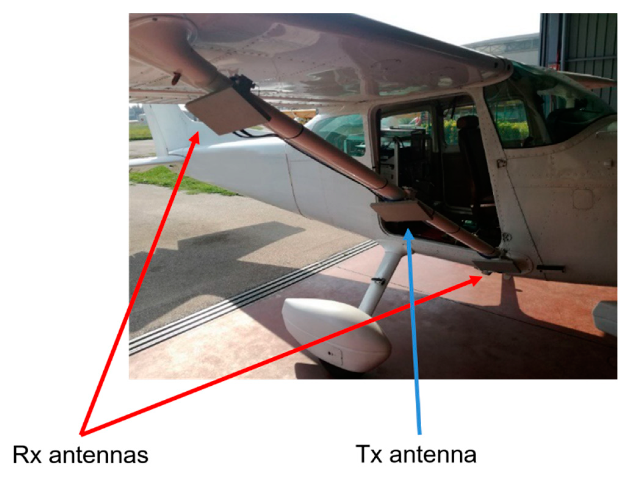
The AXIS system mounts three X-Band commercial off-the-shelf VV polarized microstrip antennas. They are very compact and light: each of them is mounted in a 24.6 × 12.6 × 1.5 cm radome with an overall weight of 420 g.
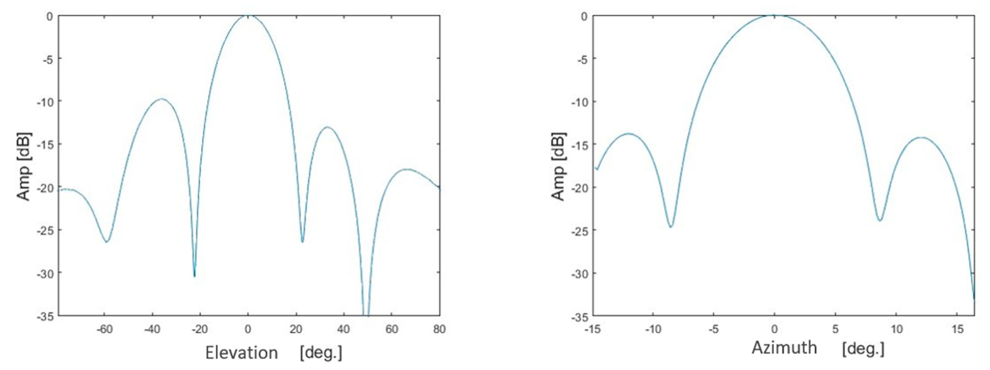
The antenna parameters were measured in the anechoic chamber of the Università degli Studi di Napoli “Parthenope”. They are practically the same for the three antennas. As an example, we report in Figure 1 the elevation and azimuth cuts of the (normalized) radiation pattern relevant to one of the three antennas, namely that with serial number MAA-935985-V. In this case, the measured gain [31] is 24.7 dB; the measured half power beamwidth [31] is equal to 19.2° in elevation and 7.4° in azimuth. When considering the squared pattern (to account for the two-way signal path), these values decrease to 14° and 5.4°, respectively.
It is finally remarked that in the anechoic chamber was also carried out a very accurate measurement of the phase center position of each radar antenna, see [32].
2.3. Interferometric Layout
The AXIS system is equipped with a single-pass interferometric layout. As remarked above, like any conventional FMCW system, AXIS is a bistatic radar; that is, the Tx antenna is not also used to receive. Accordingly, three radar antennas, one Tx and two Rx, are necessary to obtain a single-pass interferometric configuration.
As specified above, the system is currently mounted on board a Cessna 172 aircraft. For this airplane, the three antennas are mounted on the strut of the right wing by means of customized camera mounts; see Figure 2. By doing so, the antennas exhibit a pointing angle in the elevation plane equal to 45 degrees; moreover, the interferometric baseline between the two Rx devices is equal to 1.75 m. For flight altitudes of 1 Km, 2 Km, and 3 Km, which are typical of comparatively small aircrafts, this baseline leads to the height of ambiguity values [1] reported in Figure 3.
The lever arms, namely, the distances between the antennas’ phase centers and the reference center of the navigation unit, were measured using the theodolite technique before the airborne mission [9,33].
Some considerations on the strategy adopted to obtain the AXIS interferometric layout are now in order.
First of all, we underline that one of the reasons why we chose to mount the antennas on the wing strut is that this is one of the least flexible structures of the aircraft. This allows us to limit the problems related to the presence of small deformations unavoidably occurring on the aircraft body during flight. We are thus quite confident that the difference between the in-flight and measured lever arms is negligible; in any case, this difference is reasonably within the accuracy of the adopted theodolite measurement equipment.
Second, we remark that the three camera mounts shown in Figure 2 are fixed separately. Accordingly, the solution adopted to install the three antennas could not ensure sufficiently accurate (that is, within the accuracy of the adopted theodolite measurement equipment) repeatability of the overall obtained antenna layout (that is, the relative positions of the antennas as well as their orientations in azimuth and elevation). For this reason, with the architectural solution shown in Figure 2 it is preferable to repeat the measurement of the lever arms for each acquisition campaign. This, of course, may represent a strong limitation on the flexible use of the radar, especially if we intend to mount it on board the aircraft only when required. Indeed, in an operative crisis scenario, in which fast data acquisition and processing could be requested, the lever arms measurement operation could dramatically delay the beginning of the flight mission and data processing (we recall that precise knowledge of the lever arms is necessary to ensure accurate airborne SAR data focusing [20]). To overcome this limitation, for future missions, a rigid mechanical framework embedding the three antennas (and tailored to any Cessna 172 model) was designed and built. In this way, at worst a constant (and reasonably small) bias between the overall antennas’ frame and the IMU reference center will occur when re-installing the antennas before each mission. We are quite confident that this will make it unnecessary to measure the lever arms after each antenna installation. In any case, a deeper analysis of these kinds of issues is a matter of current investigation.
2.4. Radar
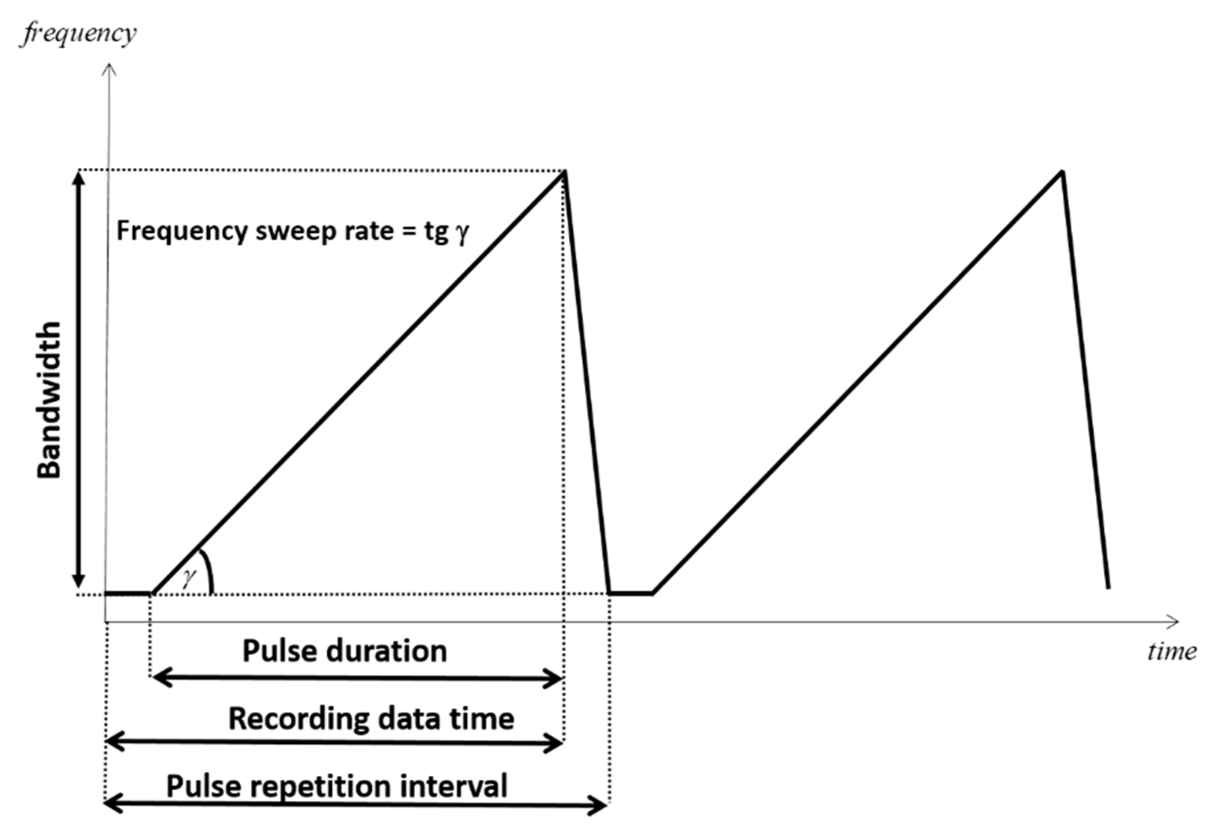
The AXIS radar exploits FMCW technology, which allows for operating in a high-resolution mode though exploiting the comparatively low ADC sampling frequency and low data rate. The main radar parameters are collected in Table 3. Note in particular that, following the notation largely used in the literature [29,30], in the table we have used some terms (Pulse repetition interval, Pulse duration, Pulse repetition frequency) borrowed from pulse radar jargon. The meaning of these terms for FMCW radar is clarified in Figure 4, which shows the temporal behavior of the frequency of the signal continuously transmitted by such kinds of radars. In this regard, note in particular that the pulse repetition frequency is equal to the inverse of the pulse repetition interval. In the specific case of the AXIS system, the recording data time is 605 µs, while the frequency sweep rate, accurately measured following the procedure in [34], is 3.336 × 10¹¹ s−2, which leads to a maximum range distance of about 5615 m recordable by the radar. Moreover, the sampling rate is 25 MHz, while the bandwidth of the transmitted signal is 200 MHz, leading to a slant range resolution of about 0.75 m [30].
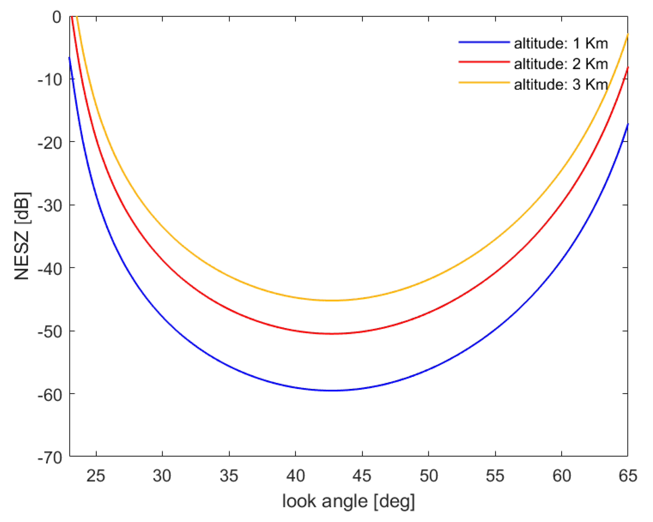
The Noise Equivalent Sigma Zero (NESZ) [29] of the system was computed according to the antenna gain measurements carried out in the laboratory (see previous section) and the radar components’ specifications. The behavior of the NESZ versus the radar look angle is reported in Figure 5 for different flight altitudes.
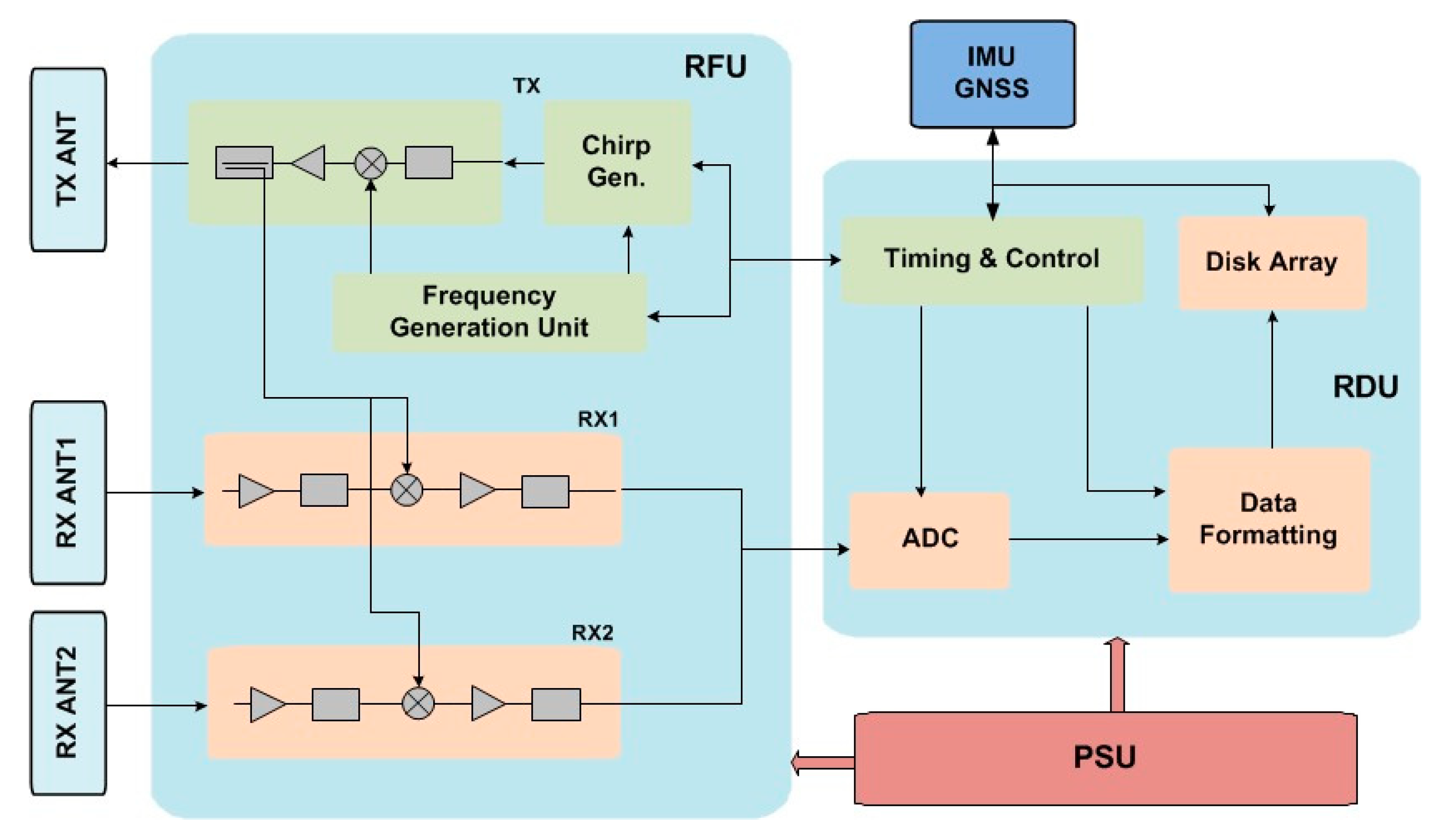
A block diagram of the radar module is shown in Figure 6. As can be seen in the figure, it consists of three main blocks, namely, the Radar Digital Unit (RDU), the Radio Frequency Unit (RFU), which is connected to the three antennas, and the Power Supply Unit (PSU). In particular, the RDU is fully programmable and allows for setting the acquisition parameters, the generation timing, and the data handling. It also includes the ADC and the data storage unit. The RFU includes the frequency generation unit (which generates all the synchronization and radio frequency signals) and the chirp generator unit (which generates the low-frequency modulated chirp signal by means of digital direct synthesis technology). The RFU also includes the power amplifier, the Up/Down converter, and an antenna front-end. The PSU provides the power supply to the whole system by 24–28 V DC internal power. It is completely autonomous and does not affect the aircraft DC bus power. The navigation system is directly connected to the RDU by means of a specific interface; all the navigation data are synchronized with the radar pulses and embedded in the output data. The radar module has a weight of approximately 30 kg (comprising the PSU), and it is accommodated in a rack whose size is about 50 cm × 50 cm × 65 cm. Due to the comparatively low weight and compactness of the radar module, the AXIS system can be mounted on board small aircraft and helicopters. As specified above, the system is currently mounted on board a Cessna 172 aircraft. In particular, the rack that includes the radar module and the navigation system is installed in the aircraft cabin, in place of the two rear passenger seats.
3. Experimental Results
In this section, we present the results relevant to the SAR data acquisition campaign carried out using the AXIS system over the Salerno area, Italy, in April 2018. More specifically, a flight campaign consisting of six overlapping flight circuits was scheduled, each of them containing two antiparallel linear tracks of about 20 km. In other words, we planned to collect SAR data from 12 flight tracks: 6 overlapping tracks from southeast (SE) to northwest (NW) and 6 overlapping tracks from NW to SE. In Figure 7, which shows an optical image of the test area, the actually flown circuits (obtained through the navigation data recorded during the overall campaign) are depicted with yellow lines.
Besides the flight campaign, we also performed a ground campaign aimed first of all at measuring the antennas’ lever arms, in order to provide the information necessary to accurately process the radar data [35,36]. As specified above, such measurements were carried out very precisely through a Total Station Theodolite. The ground campaign was also aimed at providing a number of sound ground control points to assess the quality of the obtained SAR images and interferometric products. To do this, 10 CRs (5 for the NW–SE and 5 for the SE–NW flight tracks) were deployed over the area illuminated by the radar, and their positions were accurately measured by means of D-GPS surveys.
The main SAR acquisition parameters are summarized in Table 4. We recall that the minimum recordable range for an FMCW system is 0 m. In our case, we focused only a range portion of the overall acquired data by setting a near (slant) range equal to about 2478 m, corresponding to a (mean) look angle of about 20 degrees.
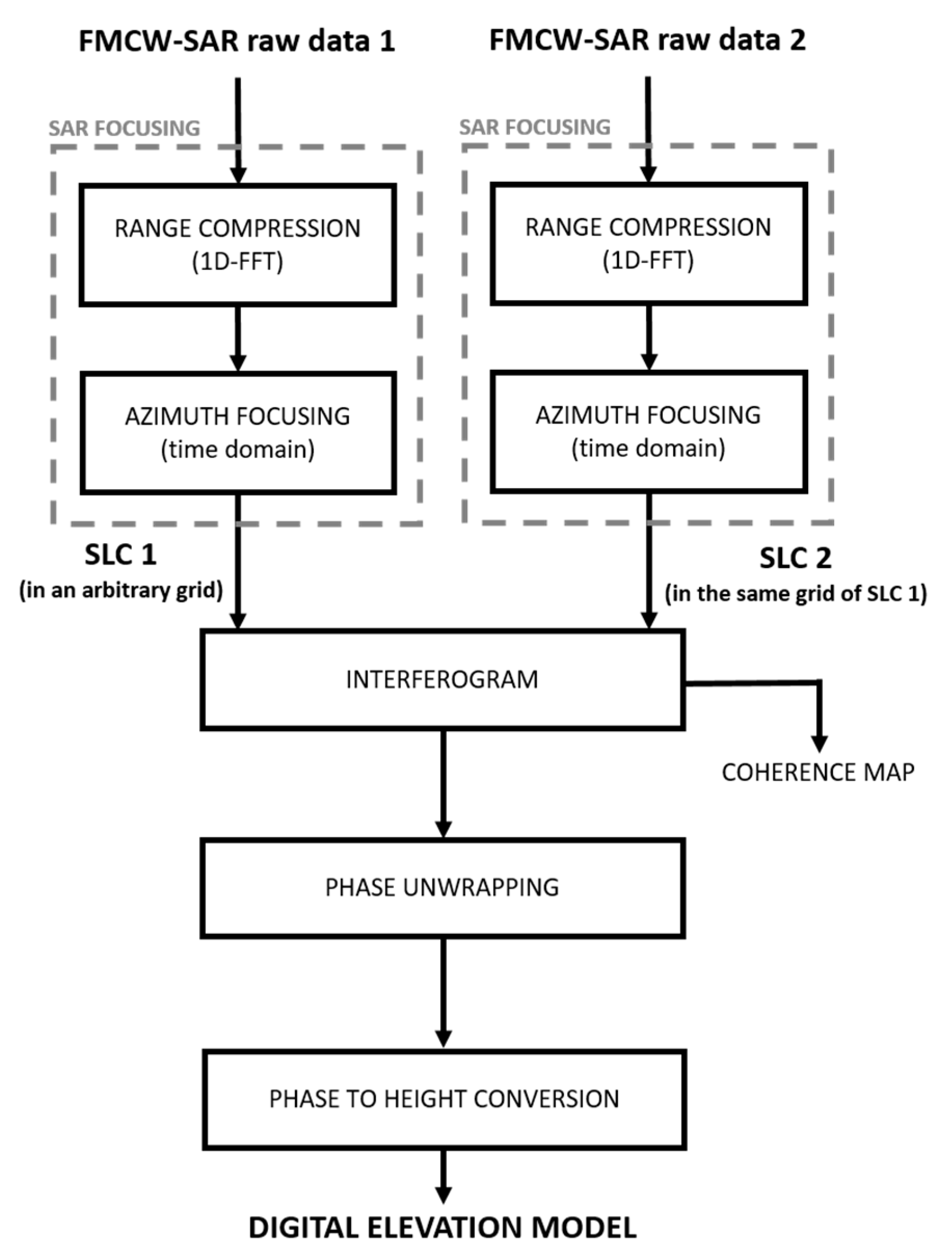
In Figure 8, a block diagram of the adopted InSAR processing chain is depicted. In particular, the range compression of FMCW SAR data simply requires a Fourier transform of each range line [30]. The azimuth compression step was carried out through a time-domain Back Projection (BP) strategy [35,36] by exploiting the information provided by the measured antennas’ phase centers and lever arms, the navigation data and an external DEM, namely the SRTM one [37], of the observed area. The adopted processing strategy allowed us to avoid application of the approximations [38] necessary to implement frequency-domain focusing approaches with integrated motion compensation [39,40]. This, of course, involves an increase of the computational burden, but this can be managed by means of parallel computing strategies that, for the time-domain approaches, are very easy to implement. Moreover, like all the time-domain focusing algorithms based on BP approaches, our processing strategy allowed us to focus all the SAR images in a common output grid, thus avoiding the need to apply the co-registration step [1] to generate the SAR interferograms. Except for this latter processing step, standard InSAR processing [1] was applied for the generation of the interferometric products. Hereafter, we focus our attention on a single-pass interferometric dataset related to a flight track flown from SE to NW. More specifically, we first analyze the obtained amplitude SAR images and then the interferometric products.
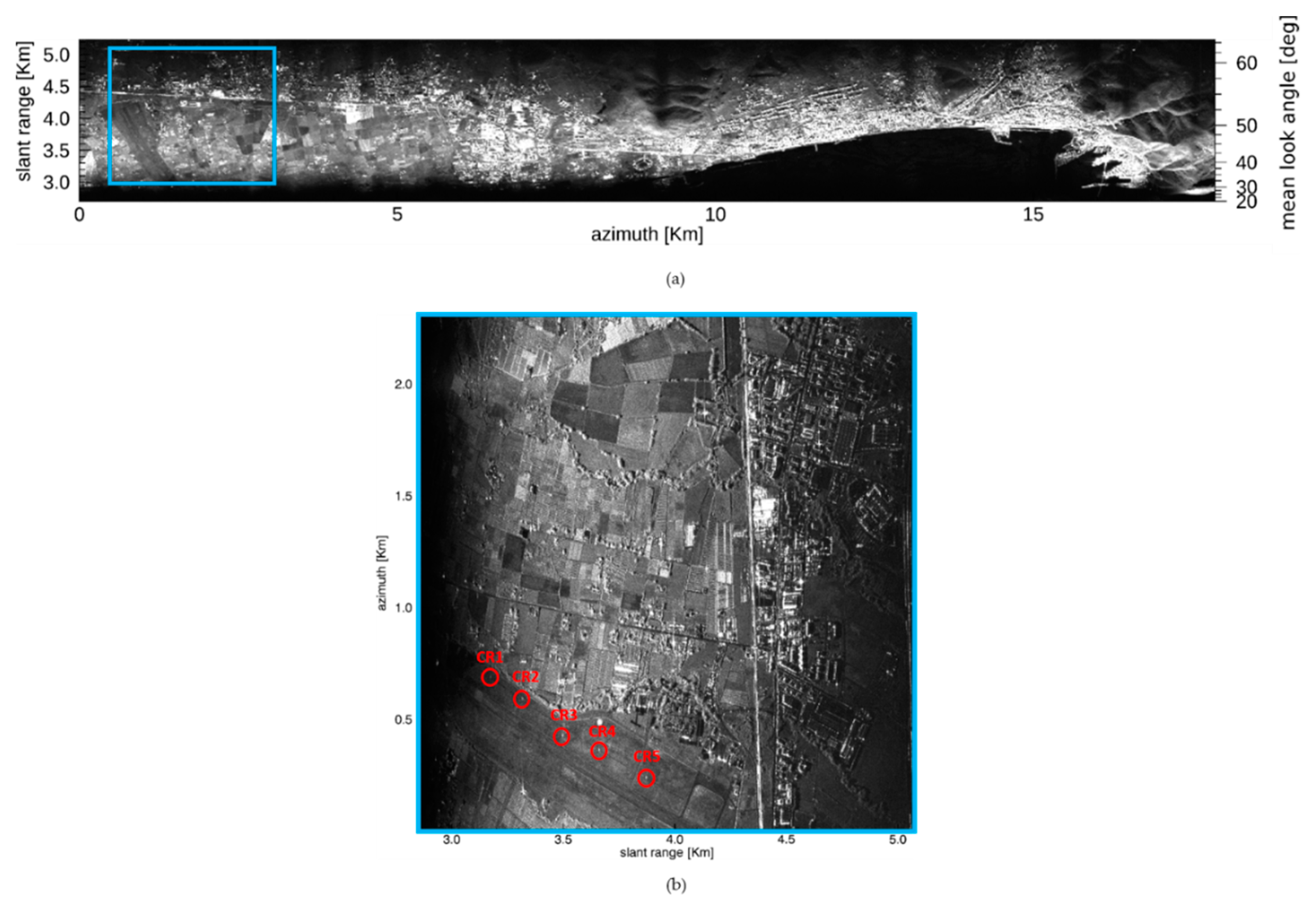
Figure 9 shows the amplitude of the multi-look complex (MLC) SAR image relevant to the whole track. The image is focused in an output grid coincident with the radar one (that is, slant range and azimuth). Note that in the right vertical axis of the figure is specified the (mean) look angle corresponding to the range coordinate reported in the left vertical axis. We remark that in the figure, a 10 range × 10 azimuth pixel averaging window was applied for visualization purposes, obtaining 15 m × 16 m pixel spacing. The details of the main processing parameters are reported in Table 5. From the figure we note amplitude decay for small values (approximately less than 25 degrees) and high values (approximately greater than 60 degrees) of the (mean) look angle. This is in agreement with the NESZ curves of Figure 5 (we recall that for the considered flight altitude, the region of our interest in Figure 5 lies between the red and yellow curves).
Figure 9b instead reports a multi-look amplitude SAR image of a small area around Salerno’s airport (see the light blue box in Figure 9a), which was processed at a higher resolution (see again Table 5). Note, in particular, that a 2 range × 10 azimuth pixel averaging window was applied in the figure for visualization purposes, obtaining 1.5 m × 1.6 m pixel spacing. All the five deployed CRs relevant to the SE–NW track are present in this area; they are highlighted in the figure with red circles.
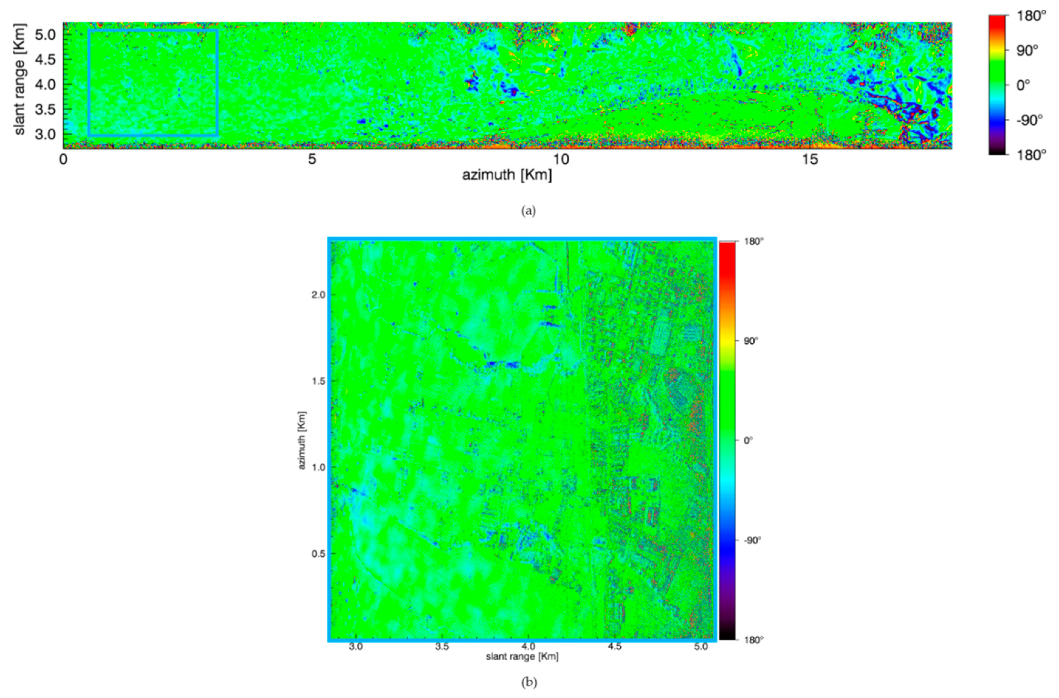
Processing parameters relevant to both images are listed in Table 5. For both images, the output grid coincides with the radar one (range–azimuth). Starting from the single-pass data pair focused with the processing parameters of Figure 9a, we obtained the wrapped interferogram and the corresponding coherence map shown in Figure 10a and Figure 11a, respectively. Note that, as in Figure 9a, a 10 range × 10 azimuth pixel averaging window was applied to generate these two maps. Figure 10b and Figure 11b instead report the interferogram and the corresponding coherence map obtained starting from the single-pass data pair focused with the processing parameters of Figure 9b. As in Figure 9b, a 2 range × 10 azimuth pixel averaging window was applied to generate these two maps. It is stressed that to obtain the interferometric products shown in Figure 10 and Figure 11, besides the averaging window described above, we did not apply any additional filter aimed at limiting the noise effects. It is finally noted that in all the interferograms shown, we removed the topographic component provided by the external SRTM DEM used during the focusing step.
Starting from the wrapped interferograms of Figure 10, we applied the phase unwrapping procedure from [41,42]. Then, we estimated the resulting unknown phase offset present in the unwrapped interferograms by applying the Phase-Based Estimate (PBE) procedure detailed in [33,43,44] and exploiting the D-GPS measurements relevant to the CRs. Thereafter, we carried out the phase-to-height conversion [1] to generate the InSAR DEM. The result relevant to the low-resolution interferogram of Figure 10a is displayed in Figure 12 on a geographic grid and superimposed upon an optical image of the overall test area.
A quantitative assessment of the presented SAR products was performed by exploiting the five CRs shown in Figure 9b, along with the in situ D-GPS measurements relevant to their positions. More specifically, we carried out three different experiments by exploiting the high-resolution SAR image and interferogram generated with the processing parameters considered in Figure 9b and Figure 10b.
In the first experiment, we measured the geometric resolution of the Single Look Complex (SLC) image in correspondence with the five CRs. The achieved results are listed in Table 6. We recall that the expected values are 0.33 m in azimuth and 0.75 m in range (see Table 5). In particular, we measured a mean azimuth resolution of 0.36 m with a standard deviation of 0.008 m, and a mean range resolution of 0.74 m with a standard deviation of 0.04 m. Note that no filtering (such as Hamming [1]) aimed at reducing the side lobe level of the point spread function (PSF) was applied. It is evident from Table 6 that the measured resolutions are very close to the expected theoretical ones. Moreover, it can also be noted that in most cases (with the exception of CR3) the measured range resolution is finer than the expected theoretical one. This is due to the fact that we chose the output geometry of the focused image according to the mean antenna pointing direction along the azimuth direction. Accordingly, the output geometry (also named processing geometry in the literature [45]) may be different from the acquisition geometry dictated by the actual antenna pointing direction within the azimuth aperture from which a generic target is illuminated. When this happens, the two-dimensional PSF relevant to the target is rotated with respect to the output grid [45]. As a consequence, measuring the resolution of the two-dimensional PSF along the azimuth and range directions of the output grid leads to an apparent improvement of the lower resolution (in our case, the range one; see Table 5) and an apparent impairment of the higher resolution (in our case, the azimuth one; see Table 5).
As a second experiment, we measured the planar (that is, in the azimuth and range directions) positioning accuracy of the Single Look Complex (SLC) image in correspondence with the five CRs. To do this, we applied the backward geocoding procedure [1] to the D-GPS positions of the CRs, thus calculating their expected azimuth and range coordinates in the considered SAR image output grid. Then, we compared these coordinates with those of the CRs imaged in the SLC image. The range and azimuth misalignments measured for all the CRs are listed in Table 6. In particular, we measured a mean azimuth misalignment of 0.39 m with a standard deviation of 0.04 m, and a mean range misalignment of 0.26 m with a standard deviation of 0.10 m. It is noted that in the range direction the measured mean misalignment is lower than the resolution, whereas in the azimuth direction it is comparable to the resolution.
As a third experiment, we provided a first estimate of the vertical accuracy of the AXIS InSAR DEM. To do this, we compared the height values achieved on the AXIS InSAR DEM, in correspondence with the CR positions, with the D-GPS ones. The results are again collected in Table 6. In particular, we measured a mean vertical error of 0.20 m with a standard deviation of 0.41 m.
4. Discussion
A discussion concerning the presented results is now addressed.
In the previous section, to carry out the analysis of the AXIS performances, we have exploited five CRs properly deployed within the illuminated area and the D-GPS surveys of their positions. In this way, we have obtained a number of ground measurements that may be considered with good approximation as the ground truth.
In correspondence with this set of ground reference points we first measured the geometric resolution of the focused AXIS images. In particular, for the SLC image we have obtained mean geometric resolutions of 0.36 m (azimuth) × 0.74 m (range), with standard deviations of 0.008 m (azimuth) and 0.04 m (range). These values turned out to be practically the same as the expected theoretical ones.
Then, we measured the planar (that is, in the azimuth and range directions) positioning accuracy of the focused AXIS images, obtaining for the SLC image a mean positioning misalignment of 0.39 m (azimuth) × 0.26 m (range) with standard deviations of 0.04 m (azimuth) and 0.10 m (range). Finally, we compared the D-GPS measurements of the positions of the CRs with the height values of the single-pass InSAR AXIS DEM in correspondence with the imaged CRs, obtaining a mean vertical error of 0.20 m with a standard deviation of 0.41 m. From these results it turns out that some systematic errors seem to affect the obtained measurements. These errors are, however, tolerable, since the mean range misalignment (0.26 m) is less than the range resolution and spacing (0.75 m) of the system; the mean azimuth misalignment (0.39 m) is comparable to the azimuth resolution (0.33 m) of the system; and the mean vertical error is just 0.20 m. It is likely that these three systematic effects are somehow related. Given the amount of the mean range bias, one possible explanation could be the presence of an uncompensated internal radar delay. In any case, further investigations on this issue are a matter of current work.
Summing up, the measured imaging and topographic mapping capabilities of the overall AXIS infrastructure (which consists of the radar system along with the complete data processing chain that leads from the acquired raw data to the generated SAR and InSAR products) well match the theoretical, expected ones.
Moreover, the imaging and topographic mapping capabilities of this low cost, compact and flexible FMCW system are comparable to those achieved using well-assessed, although more expensive, pulsed airborne X-band SAR systems, like, for instance, InSAeS4 [9]. Indeed, in [9], starting from an analysis similar to that addressed in this work for the AXIS system, it was measured for InSAeS4 a mean geometric resolution of 0.14 m (azimuth) × 0.49 m (range), a mean positioning misalignment of 0.08 m (azimuth) × 0.04 m (range) with a standard deviation of 0.07 m (azimuth) and 0.08 m (range), and a mean height error (of the obtained single-pass InSAR DEM) of −0.08 m with a standard deviation of 0.51 m.
5. Conclusions
In this work, we presented a first assessment of the imaging and topographic mapping capabilities of the AXIS system, which is a newborn single-pass interferometric airborne FMCW SAR system developed in the frame of cooperation between a public research institute (IREA-CNR) and a private company (Elettra Microwave S.r.l.).
In particular, we showed results relevant to an acquisition campaign carried out over the Salerno area, South of Italy, in 2018, just after the system completion. More specifically, we provided a first quantitative assessment of the quality of the focused SAR images and InSAR products achieved using the AXIS system. To do this, we exploited a number of CRs properly deployed within the area illuminated by the radar and D-GPS surveys of their positions.
More specifically, in correspondence with this set of ground reference points we measured the geometric resolution and the positioning misalignment of the focused AXIS images, obtaining for the SLC image, mean geometric resolutions practically equal to the expected theoretical ones, a mean range misalignment smaller than the resolution and a mean azimuth misalignment comparable to the resolution. Moreover, we compared the D-GPS measurements of the positions of the CRs with the height values of the single-pass InSAR AXIS DEM in correspondence with the imaged CRs, obtaining a vertical error on the order of dozens of centimeters.
The presented results, aimed at providing first reference values for future research and operational activities that will be conducted with this system, already show that the imaging and topographic mapping capabilities of the AXIS system well match the theoretical, expected ones. Moreover, they are comparable to those achievable using well-assessed, although typically more expensive, pulsed SAR systems. More generally, the presented results show that the AXIS infrastructure (which consists of the radar system along with the complete data processing chain from the acquired raw data to the generated InSAR products) may represent an appealing monitoring solution for those applications that require the use of high-resolution InSAR products.
Author Contributions
Conceptualization, C.E., A.N., G.P., P.B., R.L., S.P.; Methodology, Software and Validation, C.E., A.N., P.B., S.P.; Investigation, C.E., A.N., G.P., P.B., R.L., S.P.; Data Curation, C.E., A.N., G.P., P.B., S.P.; Writing—Original Draft Preparation, C.E., A.N., S.P.; Supervision, S.P. All authors have read and agreed to the published version of the manuscript.
Funding
This work was supported in part by the Italian Department of Civil Protection (DPC) in the framework of the DPC-IREA Agreement (2019-2021) and in part by the Italian Ministry of Economic Development (MISE) in the framework of the contract “MATRAKA”. Part of the presented research has been carried out through the I-AMICA (Infrastructure of High Technology for Environmental and Climate Monitoring-PONa3_00363).
Acknowledgments
The authors thank S. Guarino, F. Parisi and M. C. Rasulo of IREA-CNR, for their support, Etabeta srl for their contribution during the ground campaign, A. Gifuni of Università degli Studi di Napoli “Parthenope” for his contribution to the antennas measurements.
Conflicts of Interest
The authors declare no conflict of interest.
References
- Franceschetti, G.; Lanari, R. Synthetic Aperture Radar Processing; CRC PRESS: New York, NY, USA, 1999. [Google Scholar]
- Moreira, A.; Prats-Iraola, P.; Younis, M.; Krieger, G.; Hajnsek, I.; Papathanassiou, K.P. A tutorial on synthetic aperture radar. IEEE Geosci. Remote Sens. Mag. 2013, 1, 6–43. [Google Scholar] [CrossRef] [Green Version]
- Krieger, G.; Moreira, A.; Fiedler, H.; Hajnsek, I.; Werner, M.; Younis, M.; Zink, M. TanDEM-X: A Satellite Formation for High-Resolution SAR Interferometry. IEEE Trans. Geosci. Remote Sens. 2007, 45, 3317–3341. [Google Scholar] [CrossRef] [Green Version]
- Torre, A.; Calabrese, D.; Porfilio, M. COSMO-SkyMed: Image quality achievements. In Proceedings of the 5th International Conference on Recent Advances in Space Technologies—RAST2011, Istanbal, Turkey, 9–11 June 2011. [Google Scholar]
- Torres, R.; Snoeij, P.; Geudtner, D.; Bibby, D.; Davidson, M.; Attema, E.; Potin, P.; Rommen, B.; Floury, N.; Brown, M.; et al. GMES Sentinel-1 Mission. Remote Sens. Environ. 2012, 120, 9–24. [Google Scholar] [CrossRef]
- Le Toan, T.; Quegan, S.; Davidson, M.W.J.; Balzter, H.; Paillou, P.; Papathanassiou, K.; Plummer, S.; Rocca, F.; Saatchi, S.; Shugart, H.; et al. The BIOMASS mission: Mapping global forest biomass to better understand the terrestrial carbon cycle. Remote Sens. Environ. 2011, 115, 2850–2860. [Google Scholar] [CrossRef] [Green Version]
- Kim, D.-J.; Hensley, S.; Yun, S.-H.; Neumann, M. Detection of Durable and Permanent Changes in Urban Areas Using Multitemporal Polarimetric UAVSAR Data. IEEE Geosci. Remote Sens. Lett. 2016, 13, 267–271. [Google Scholar] [CrossRef]
- Baqué, R.; Bonin, G.; du Plessis, O.R. The airborne SAR-system: SETHI airborne microwave remote sensing imaging system. In Proceedings of the 7th European Conference on Synthetic Aperture Radar, Friedrichshafen, Germany, 2–5 June 2008. [Google Scholar]
- Perna, S.; Esposito, C.; Amaral, T.; Berardino, P.; Jackson, G.; Moreira, J.; Pauciullo, A.; Vaz Junior, E.; Wimmer, C.; Lanari, R. The InSAeS4 airborne X-band interferometric SAR system: A first assesment on its imaging and topographic mapping capabilities. Remote Sens. 2016, 8, 40. [Google Scholar] [CrossRef] [Green Version]
- Pinheiro, M.; Reigber, A.; Scheiber, R.; Prats-Iraola, P.; Moreira, A. Generation of highly accurate DEMs over flat areas by means of dual-frequency and dual-baseline airborne SAR interferometry. IEEE Trans. Geosci. Remote Sens. 2018, 56, 4361–4390. [Google Scholar] [CrossRef] [Green Version]
- Perna, S.; Alberti, G.; Berardino, P.; Bruzzone, L.; Califano, D.; Catapano, I.; Ciofaniello, L.; Donini, E.; Esposito, C.; Facchinetti, C.; et al. The ASI Integrated Sounder-SAR System Operating in the UHF-VHF Bands: First Results of the 2018 Helicopter-Borne Morocco Desert Campaign. Remote Sens. 2019, 11, 1845. [Google Scholar] [CrossRef] [Green Version]
- Aguasca, A.; Acevo-Herrera, R.; Broquetas, A.; Mallorqui, J.J.; Fabregas, X. ARBRES: Light-Weight CW/FM SAR Sensors for Small UAVs. Sensors 2013, 13, 3204–3216. [Google Scholar] [CrossRef] [Green Version]
- Ouchi, K. Recent Trend and Advance of Synthetic Aperture Radar with Selected Topics. Remote Sens. 2013, 5, 716–807. [Google Scholar] [CrossRef] [Green Version]
- Brenner, A.R.; Roessing, L. Radar Imaging of Urban Areas by Means of Very High-Resolution SAR and Interferometric SAR. IEEE Trans. Geosci. Remote Sens. 2008, 46, 2971–2982. [Google Scholar] [CrossRef]
- Dubois-Fernandez, P.; du Plessis, O.R.; le Coz, D.; Dupas, J.; Vaizan, B.; Dupuis, X.; Cantalloube, H.; Coloumbeix, C.; Titin-Schnaider, C.; Dreuillet, P.; et al. The ONERA RAMSES SAR system. In Proceedings of the International Geoscience and Remote Sensing Symposium, Toronto, ON, CA, 24–28 June 2002. [Google Scholar]
- Ruault du Plessis, O.; Nouvel, J.; Baque, R.; Bonin, G.; Dreuillet, P.; Coulombaix, C.; Oriot, H. ONERA SAR facilities. IEEE Aerosp. Electron. Syst. Mag. 2011, 26, 24–30. [Google Scholar] [CrossRef]
- Perna, S.; Wimmer, C.; Moreira, J.; Fornaro, G. X-Band Airborne Differential Interferometry: Results of the OrbiSAR Campaign Over the Perugia Area. IEEE Trans. Geosci. Remote Sens. 2008, 46, 489–503. [Google Scholar] [CrossRef]
- Magnard, C.; Frioud, M.; Small, D.; Brehm, T.; Essen, H.; Meier, E. Processing of MEMPHIS Ka-Band Multibaseline Interferometric SAR Data: From Raw Data to Digital Surface Models. IEEE J. Sel. Top. Appl. Earth Observ. Remote Sens. 2014, 7, 2927–2941. [Google Scholar] [CrossRef]
- Schmitt, M.; Stilla, U. Maximum-likelihood based approach for single-pass synthetic aperture radar tomography over urban areas. IET Radar Sonar Navig. 2014, 8, 1145–1153. [Google Scholar] [CrossRef]
- Fornaro, G.; Franceschetti, G.; Perna, S. Motion Compensation Errors: Effects on the Accuracy of Airborne SAR Images. IEEE Trans. Aerosp. Electron. Syst. 2005, 41, 1338–1352. [Google Scholar] [CrossRef]
- Tomiyasu, K. Conceptual Performance of a Satellite Borne, Wide Swath Synthetic Aperture Radar. IEEE Trans. Geosci. Remote Sens. 1981, 2, 108–116. [Google Scholar] [CrossRef]
- Gebert, N.; Krieger, G.; Moreira, A. Multichannel azimuth processing in ScanSAR and TOPS mode operation. IEEE Trans. Geosci. Remote Sens. 2010, 48, 2994–3008. [Google Scholar] [CrossRef] [Green Version]
- De Zan, F.; Monti Guarnieri, A. TOPSAR: Terrain Observation by Progressive Scans. IEEE Trans. Geosci. Remote Sens. 2006, 44, 2352–2360. [Google Scholar] [CrossRef]
- Gebert, N.; Krieger, G.; Moreira, A. Digital beamforming on receive: Techniques and optimization strategies for high-resolution wide-swath SAR imaging. IEEE Trans. Aerosp. Electron. Syst. 2009, 45, 564–592. [Google Scholar] [CrossRef] [Green Version]
- Anantrasirichai, N.; Biggs, J.; Albino, F.; Hill, P.; Bull, D. Application of Machine Learning to Classification of Volcanic Deformation in Routinely Generated InSAR Data. J. Geophys. Res. Solid Earth 2018, 123, 6592–6606. [Google Scholar] [CrossRef] [Green Version]
- Ma, P.; Zhang, F.; Lin, H. Prediction of InSAR time-series deformation using deep convolutional neural networks. Remote Sens. Lett. 2019, 11, 137–145. [Google Scholar] [CrossRef]
- Anantrasirichai, N.; Biggs, J.; Albino, F.; Bull, D. A deep learning approach to detecting volcano deformation from satellite imagery using synthetic datasets. Remote Sens. Environ. 2019, 230, 111–179. [Google Scholar] [CrossRef] [Green Version]
- Valade, S.; Ley, A.; Massimetti, F.; D’Hondt, O.; Laiolo, M.; Coppola, D.; Loibl, D.; Hellwich, O.; Walter, T.R. Towards Global Volcano Monitoring Using Multisensor Sentinel Missions and Artificial Intelligence: The MOUNTS Monitoring System. Remote Sens. 2019, 11, 1528. [Google Scholar] [CrossRef] [Green Version]
- Richards, M.A.; Scheer, J.A.; Holm, W.A. Principles of Modern Radar: Basic Principles; SciTech Publishing: Raleigh, NC, USA, 2010. [Google Scholar]
- Meta, A.; Hoogeboom, P.; Ligthart, L.P. Signal Processing for FMCW SAR. IEEE Trans. Geosci. Remote Sens. 2007, 45, 3519–3532. [Google Scholar] [CrossRef]
- Balanis, C.A. Antenna Theory: Analysis and Design, 3rd ed.; Wiley-Interscience: New York, NY, USA, 2005. [Google Scholar]
- Esposito, C.; Gifuni, A.; Perna, S. Measurement of the Antenna Phase Center Position in Anechoic Chamber. IEEE Antennas Wirel. Propag. Lett. 2018, 17, 2183–2187. [Google Scholar] [CrossRef]
- Wimmer, C.; Siegmund, R.; Schwabisch, M.; Moreira, J. Generation of high precision DEMs of the Wadden Sea with airborne interferometric SAR. IEEE Trans. Geosci. Remote Sens. 2000, 38, 2234–2245. [Google Scholar] [CrossRef]
- Esposito, C.; Natale, A.; Palmese, G.; Berardino, P.; Perna, S. Geometric distortions in FMCW SAR images due to inaccurate knowledge of electronic radar parameters: Analysis and correction by means of corner reflectors. Remote Sens. Environ. 2019, 232, 111289. [Google Scholar] [CrossRef]
- Berardino, P.; Esposito, C.; Natale, A.; Lanari, R.; Perna, S. Airborne SAR Focusing in the Presence of Severe Squint Variations. In Proceedings of the IGARSS 2019—2019 IEEE International Geoscience and Remote Sensing Symposium, Yokohama, Japan, 28 July–2 August 2019; pp. 537–540. [Google Scholar]
- Frey, O.; Magnard, C.; Ruegg, M.; Meier, E. Focusing of airborne Synthetic Aperture Radar data from highly nonlinear flight tracks. IEEE Trans. Geosci. Remote Sens. 2009, 47, 1844–1858. [Google Scholar] [CrossRef] [Green Version]
- Rabus, B.; Eineder, M.; Roth, A.; Bamler, R. The shuttle radar topography mission—A new class of digital elevation models acquired by spaceborne radar. ISPRS J. Photogramm. Remote Sens. 2003, 57, 241–262. [Google Scholar] [CrossRef]
- Fornaro, G.; Franceschetti, G.; Perna, S. On Center-Beam Approximation in SAR Motion Compensation. IEEE Geosci. Remote Sens. Lett. 2006, 3, 276–280. [Google Scholar] [CrossRef]
- Moreira, A.; Huang, Y. Airborne SAR Processing of Highly Squinted Data Using a Chirp Scaling Approach with Integrated Motion Compensation. IEEE Trans. Geosci. Remote Sens. 1994, 32, 1029–1040. [Google Scholar] [CrossRef]
- Fornaro, G. Trajectory Deviations in Airborne SAR: Analysis and Compensation. IEEE Trans. Aerosp. Electron. Syst. 1999, 35, 997–1009. [Google Scholar] [CrossRef]
- Costantini, M. A novel phase unwrapping method based on network programming. IEEE Trans. Geosci. Remote Sens. 1998, 36, 813–821. [Google Scholar] [CrossRef]
- Dudczyk, J.; Kawalec, A. Optimizing the minimum cost flow algorithm for the phase unwrapping process in SAR radar. Bull. Pol. Acad. Sci. Tech. Sci. 2014, 62, 511–516. [Google Scholar] [CrossRef] [Green Version]
- Esposito, C.; Pauciullo, A.; Berardino, P.; Lanari, R.; Perna, S. A Simple Solution for the Phase Offset Estimation of Airborne SAR Interferograms Without Using Corner Reflectors. IEEE Geosci. Remote Sens. Lett. 2017, 14, 379–383. [Google Scholar] [CrossRef]
- Perna, S.; Esposito, C.; Berardino, P.; Pauciullo, A.; Wimmer, C.; Lanari, R. Phase Offset Calculation for Airborne InSAR DEM Generation Without Corner Reflectors. IEEE Trans. Geosci. Remote Sens. 2014, 53, 2713–2726. [Google Scholar] [CrossRef]
- Fornaro, G.; Sansosti, E.; Lanari, R.; Tesauro, M. Role of processing geometry in SAR raw data focusing. IEEE Trans. Aerosp. Electron. Syst. 2002, 38, 441–454. [Google Scholar] [CrossRef]
Figure 1.
Elevation (left) and azimuth (right) normalized radiation patterns of one of the three radar antennas of the AXIS (Airborne X-band Interferometric Synthetic Aperture Radar (SAR)) system.
Figure 1.
Elevation (left) and azimuth (right) normalized radiation patterns of one of the three radar antennas of the AXIS (Airborne X-band Interferometric Synthetic Aperture Radar (SAR)) system.

Figure 2.
Interferometric layout of the AXIS system. The light blue arrow points to the transmitting radar antenna, whereas the red arrows point to the two receiving radar antennas.
Figure 2.
Interferometric layout of the AXIS system. The light blue arrow points to the transmitting radar antenna, whereas the red arrows point to the two receiving radar antennas.

Figure 3.
Height of ambiguity of the AXIS system versus the look angle for three different flight altitudes.
Figure 3.
Height of ambiguity of the AXIS system versus the look angle for three different flight altitudes.

Figure 4.
Operating principle of a FMCW SAR.

Figure 5.
AXIS Noise Equivalent Sigma Zero (NESZ) as a function of the look angle for different flight altitudes.
Figure 5.
AXIS Noise Equivalent Sigma Zero (NESZ) as a function of the look angle for different flight altitudes.

Figure 6.
Block diagram of the AXIS system.

Figure 7.
The flight circuits (yellow lines) flown over the Salerno area, Italy, during the AXIS acquisition campaign.
Figure 7.
The flight circuits (yellow lines) flown over the Salerno area, Italy, during the AXIS acquisition campaign.

Figure 8.
Block diagram of the adopted airborne InSAR processing chain.

Figure 9.
(a) Multi-look amplitude SAR images relevant to the acquired data. A 10 range × 10 azimuth pixel averaging window was applied, obtaining 15 m × 16 m pixel spacing. (b) Multi-look amplitude image of a patch of the entire acquired strip. A 2 range × 10 azimuth pixel averaging window was applied, obtaining 1.5 m × 1.6 m pixel spacing. Red circles indicate the Corner Reflectors’ (CRs’) positions.

Figure 10.
(a) Multi-look interferogram obtained from the single-pass data pair focused with the processing parameters of Figure 9a. A 10 range × 10 azimuth pixel averaging window was applied, obtaining 15 m × 16 m pixel spacing. (b) Multi-look interferogram obtained from the single-pass data pair focused with the processing parameters of Figure 9b. A 2 range × 10 azimuth pixel averaging window was applied, obtaining 1.5 m × 1.6 m pixel spacing.

Figure 11.
(a) Coherence map relevant to the interferogram of Figure 10a. (b) Coherence map relevant to the interferogram of Figure 10b.

Figure 12.
InSAR DEM obtained starting from the low-resolution interferogram considered in Figure 10a. The DEM was geocoded and superimposed over a Google Earth image.
Figure 12.
InSAR DEM obtained starting from the low-resolution interferogram considered in Figure 10a. The DEM was geocoded and superimposed over a Google Earth image.


Table 1.
Airplane parameters.
| Model | Cessna 172 |
| Propulsion | 1 Lycoming IO-360-L2A |
| Velocity | up to 228 km/h |
| Endurance | 5 h |
Table 2.
Absolute Accuracy Specifications (RMS) + of the Inertial Measurement Unit (IMU) *.
| Position | 0.05 m |
| Velocity | 0.005 m/s |
| Roll and Pitch | 0.005° |
| True Heading | 0.008° |
+ Root Mean Square. * after post-processing integration with GNSS data.
Table 3.
Radar parameters.
| Radar technology | FMCW |
| Transmitted power | 5 W |
| Carrier frequency | 9.55 GHz |
| Bandwidth | 200 MHz |
| Pulse repetition frequency | 1200 Hz |
| Pulse repetition interval | 833.33 µs |
| Pulse duration | 600.184 µs |
| Recording data time | 605.00 µs |
| Sampling rate | 25 MHz |
| Frequency sweep rate | 3.336 × 10¹¹ s−2 |
| Range pixel spacing | 0.74 m |
| Maximum recordable range | 5615 m |
| Number of antennas | 3 |
| Polarization | VV |
Table 4.
SAR acquisition parameters.
| Flight altitude | 2500 m |
| Mean platform velocity | 48 m/s |
| Azimuth pixel spacing * | 0.04 m |
* Raw data.
Table 5.
SAR data processing parameters relevant to the results collected in Figure 9a,b.
Table 5.
SAR data processing parameters relevant to the results collected in Figure 9a,b.
| Parameters | Figure 9a | Figure 9b |
|---|---|---|
| Azimuth sampling (output grid) | 1.6 m | 0.16 m |
| Azimuth resolution | 1.75 m | 0.33 m |
| Azimuth resolution (MLC) | 16 m | 1.6 m |
| Range sampling (output grid) | 1.5 m | 0.75 m |
| Range resolution | 1.5 m | 0.75 m |
| Range resolution (MLC) | 15 m | 1.5 m |
Table 6.
Measurements on CRs.
| Azimuth Resolution | Range Resolution | Azimuth Misalignment | Range Misalignment | Height Error | |
|---|---|---|---|---|---|
| [m] | [m] | [m] | [m] | [m] | |
| CR 1 | 0.36 | 0.72 | 0.32 | 0.21 | −0.14 |
| CR 2 | 0.36 | 0.74 | 0.43 | 0.27 | 0.66 |
| CR 3 | 0.36 | 0.80 | 0.42 | 0.26 | −0.15 |
| CR 4 | 0.38 | 0.74 | 0.37 | 0.42 | 0.65 |
| CR 5 | 0.36 | 0.70 | 0.41 | 0.15 | 0.01 |
| μ | 0.36 | 0.74 | 0.39 | 0.26 | 0.20 |
| σ | 0.008 | 0.04 | 0.04 | 0.10 | 0.41 |
μ and σ indicate the mean and the standard deviation, respectively, of the achieved results.
© 2020 by the authors. Licensee MDPI, Basel, Switzerland. This article is an open access article distributed under the terms and conditions of the Creative Commons Attribution (CC BY) license (http://creativecommons.org/licenses/by/4.0/).
Share and Cite
MDPI and ACS Style
Esposito, C.; Natale, A.; Palmese, G.; Berardino, P.; Lanari, R.; Perna, S. On the Capabilities of the Italian Airborne FMCW AXIS InSAR System. Remote Sens. 2020, 12, 539. https://0-doi-org.brum.beds.ac.uk/10.3390/rs12030539
AMA Style
Esposito C, Natale A, Palmese G, Berardino P, Lanari R, Perna S. On the Capabilities of the Italian Airborne FMCW AXIS InSAR System. Remote Sensing. 2020; 12(3):539. https://0-doi-org.brum.beds.ac.uk/10.3390/rs12030539
Chicago/Turabian StyleEsposito, Carmen, Antonio Natale, Gianfranco Palmese, Paolo Berardino, Riccardo Lanari, and Stefano Perna. 2020. "On the Capabilities of the Italian Airborne FMCW AXIS InSAR System" Remote Sensing 12, no. 3: 539. https://0-doi-org.brum.beds.ac.uk/10.3390/rs12030539
Note that from the first issue of 2016, this journal uses article numbers instead of page numbers. See further details here.