Article

Crop Growth Monitoring with Drone-Borne DInSAR

1
School of Electrical and Computer Engineering, University of Campinas—UNICAMP, Campinas 13083-852, Brazil
2
School of Agricultural Engineering, University of Campinas—UNICAMP, Campinas 13083-875, Brazil
3
National Institute for Space Research—INPE, São José dos Campos 12227-010, Brazil
4
Radaz Indústria e Comércio de Produtos Eletrônicos Ltda., São José dos Campos 12244-000, Brazil
*
Author to whom correspondence should be addressed.
Submission received: 31 December 2019 / Revised: 30 January 2020 / Accepted: 3 February 2020 / Published: 12 February 2020

Abstract

:
Accurate, high-resolution maps of for crop growth monitoring are strongly needed by precision agriculture. The information source for such maps has been supplied by satellite-borne radars and optical sensors, and airborne and drone-borne optical sensors. This article presents a novel methodology for obtaining growth deficit maps with an accuracy down to 5 cm and a spatial resolution of 1 m, using differential synthetic aperture radar interferometry (DInSAR). Results are presented with measurements of a drone-borne DInSAR operating in three bands—P, L and C. The decorrelation time of L-band for coffee, sugar cane and corn, and the feasibility for growth deficit maps generation are discussed. A model is presented for evaluating the growth deficit of a corn crop in L-band, starting with 50 cm height. This work shows that the drone-borne DInSAR has potential as a complementary tool for precision agriculture.

Graphical Abstract

1. Introduction

Agriculture has a vital role in the economic stability and social development of a country. Effective agricultural management is essential to reduce costs and increase production. The monitoring of crop growth shall be done continuously for accurate support of decision-making [1]. Remote sensing has been an important tool for soil and crop monitoring. Optical remote sensing is widely used; nonetheless, synthetic aperture radar (SAR) remote sensing does not depend on weather conditions or sunlight. Moreover, the radar wavelength is approximately one million times greater than the wavelength of optical systems and provides complementary information about the agriculture parameters.
Several studies have shown the SAR remote sensing capabilities in growth monitoring of various crops [2,3] and crop classification [4,5,6]. Crop growth monitoring has been explored by using techniques based on statistical analysis between radar backscattering and crop height [2,3,7], with the use of techniques like interferometric SAR (InSAR) [8], polarimetric decomposition [9], polarimetric interferometric SAR (Pol-InSAR) [10] and differential SAR Interferometry (DInSAR) [10]. The DInSAR methodology presents high accuracy and spatial resolution, as it takes advantage of the phase difference between images. The most popular application of the DInSAR is the estimation of subsidence maps with millimetric accuracy. Relevant DInSAR works using satellites appeared in 1989, in 2003, using aircraft, and in 2019, employing drone-borne systems [11].
This article reports a first-stage crop growth estimation based on SAR experimental data from several circular flight surveys carried out over a test area of the School of Agricultural Engineering of the University of Campinas (UNICAMP) in Campinas, Brazil. It also proposes a model to estimate the corn crop growth, considering different stages of crop phenology. The types of flight surveys are discussed, and a growth map for a corn crop is presented. The drone-borne system presented in [12] was chosen to carry out the DInSAR procedures here reported, due to the following reasons:
  • Crop growth monitoring requires spatial resolution of 1 m or less, a growth measurement accuracy of centimeters, short revisit time and an adequate radar wavelength. The drone-borne solution easily fulfills these requirements.
  • Satellite-based DInSAR cannot satisfy all the requirements mentioned above.
  • Aircraft-based DInSAR can meet those conditions; however, the survey costs are not economically feasible for both the research work and the operational case.
This paper is divided as follows. Section 2 presents the drone-borne SAR system; the basics of SAR imaging; a summary of the DInSAR theory; the proposed model for estimating corn crop growth, considering backscattering contribution; a brief description of the experimental site; an outline of the field measurement process; the data acquisition plan for the drone-borne SAR; and the procedures for data processing. Section 3 shows the experimental results, consisting of acquired drone-borne SAR images, and both qualitative and quantitative validations of the attained growth maps. Section 4 discusses those results, and Section 5 presents the authors’ conclusions.

2. Materials and Methods

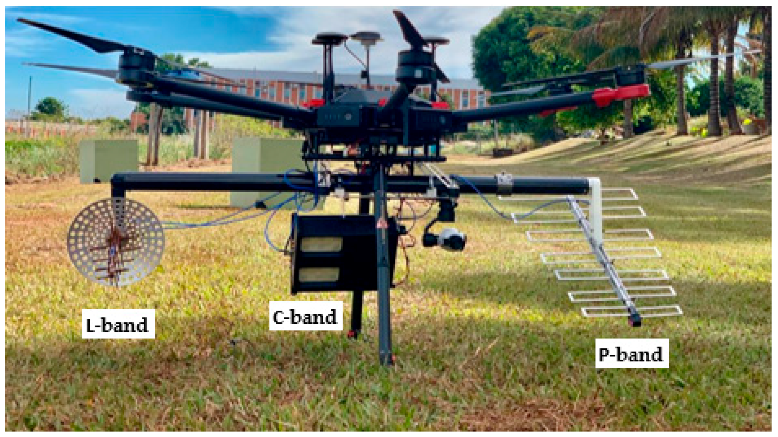
2.1. Drone-Borne SAR System

The radar prototype, described in [12] and shown in Figure 1, operates in three bands—P, L and C—with five channels: two interferometric C-band antennas, two polarimetric L-band antennas and one P-band antenna. This work only shows results for the DInSAR with the L-band HH-polarization, which corresponds to the transmission and reception of signals with horizontal polarization. The two interferometric C-band antennas are used for calculating the digital surface model, DSM, which is then used in the DInSAR calculation. Nominal height accuracy is better than 1 m RMS with a spatial resolution of 2 m. Table 1 shows the main parameters of radar acquisition for the L-band HH-polarization.
The Motion Sensing System (MSS), which includes a single channel GNSS receiver and an inertial measurement unit (IMU), is integrated into the radar, as shown in [12]. There is also a ground station with a single channel GNSS, to provide differential GNSS processing.

2.2. SAR Imaging

A circular flight pattern was chosen for generating the growth maps presented in this work. This flight geometry provides images with high resolution, which is given by the following [13]:
δ 1.2 c π cos ( θ e ) f c ,
where c is the speed of light, fc is the signal’s central frequency and θe is the depression angle. Expression (1) is valid for both directions of the ground plane. Additionally, the circular flight pattern helps to reduce shadow effects in the processed image, since it can provide full aspect coverage of the targets of interest [14].
The images were processed by using a time-domain back-projection algorithm, which is a method that is easily applied to nonlinear flight patterns. Let r l be a radar position along the flight track, and let p m n be the location of a particular pixel on the image sample grid. The back-projected signal is calculated as follows [15]:
s ( p m n ) = l g ( r l , R l m n ) e x p ( j 2 k c R l m n ) ,
where kc is the central wavenumber, and R l m n = | r l p m n | .

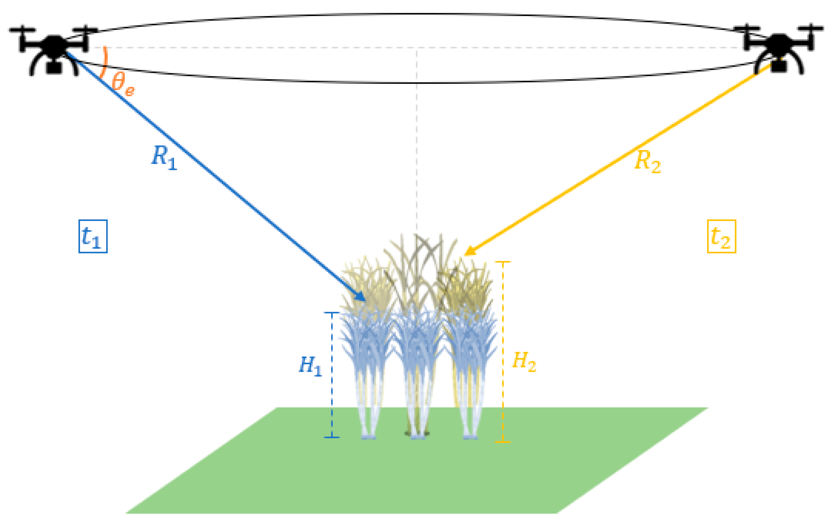
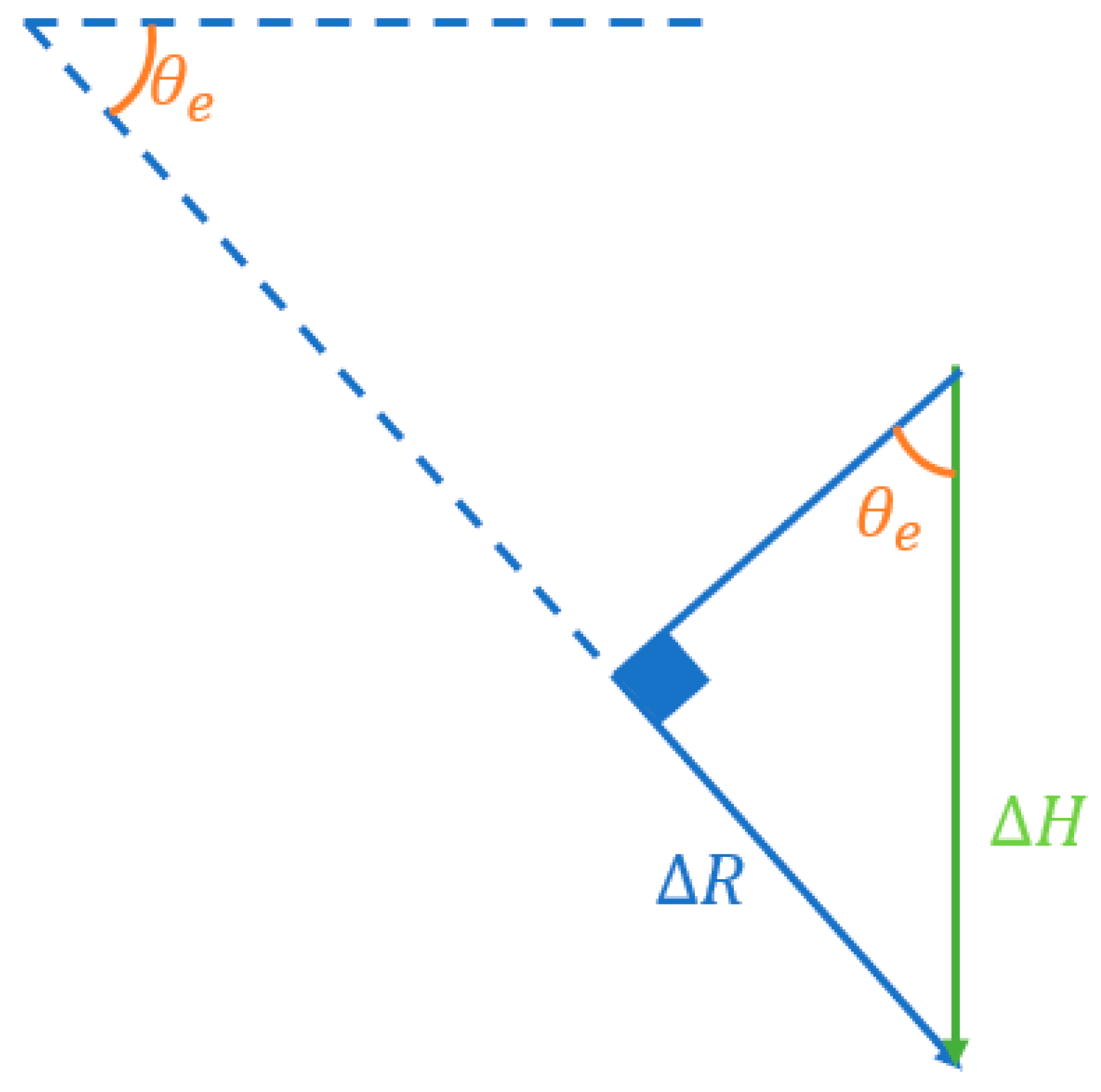
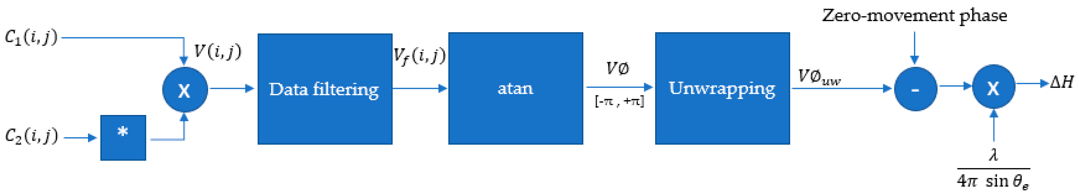
2.3. DInSAR Theory Description

DInSAR is a type of interferometry that provides information on the terrain height displacement between two flights, at different times, following the same flight path. In the DInSAR case, there is no interferometric baseline, so a topographic map is not possible. However, a terrain height displacement over time is perceptible [16]. In the present case, the analyzed terrain is a crop area.
Figure 2 presents a circular flight pattern over a crop field. The first survey is carried out at a time t1. The second survey follows the same circular flight pattern of the first flight and occurs at a time t2. Due to drone instability and weather conditions, the flight patterns are not identical but very similar.
In this example, consider that a first flight is performed on time t1, during which the crop height is H1, corresponding to a range R 1 from the radar. Then, on time t2, another flight is executed, when the crop height is now H2, and is at a range R 2 from the radar. Let Δ R = R 2 R 1 be the difference in radar range, and let Δ H = H 2 H 1 be the growth of the corn crop between these two surveys. It is possible to establish a relationship between these quantities, as shown in Figure 3.
The relationship between height and range is given by the following:
Δ H = Δ R s i n θ e ,
where θe is the depression angle. As the drone navigation system performs flight tracks with a position accuracy of about 20 cm at 120 m height, the flight tracks on different dates are assumed to be identical and, therefore, θe is virtually the same for any flight. The relationship between the radar range, Δ R , and the phase, Δ , can be described as follows [17]:
Δ R = λ 4 π Δ .
For every point of interest in the image sample grid, the mean value of θe is calculated from the contributions of the depression angles at each drone position along the flight track. If the radar antenna does not illuminate the point of interest at a given drone position, the corresponding contribution is not taken into account. This assessment is based on the antenna aperture angles in azimuth and elevation, considering a circular flight path.
In order to calculate the phase difference between both radar images, it is necessary to determine the phase corresponding to a null vertical displacement or “zero-movement” [16]. That is, it is required to find the phase corresponding to an object within the image for which there was certainly no displacement between the acquisition flights. The zero-movement phase is then subtracted from the phase difference information. Figure 4 shows the scheme used for processing the phase data obtained from two radar images.
After performing back-projection processing, two images were acquired that have amplitude and phase information. The information of interest is the phase difference between them, calculated as follows:
V ( i , j ) = C 1 ( i , j ) × C 2 * ( i , j ) ,
where C 1 ( i , j ) and C 2 ( i , j ) represent the two images, and V ( i , j ) is the image containing the phase difference information. Then, the real and imaginary components of V ( i , j ) are filtered, and so the phase information V is obtained. The next step is to get V u w from V by using a technique known as phase unwrapping [18]. After that, the zero-movement phase is subtracted. Finally, the resultant value is multiplied by a factor based on Equations (3) and (4), to obtain the vertical displacement or interferometric height difference, Δ H .

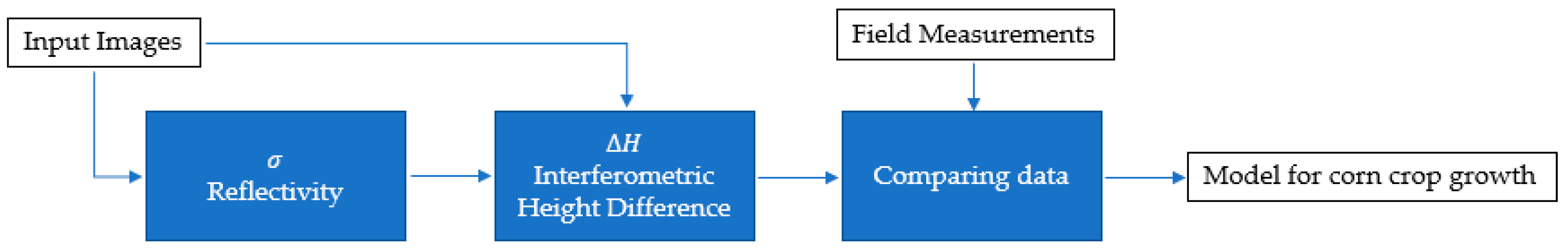
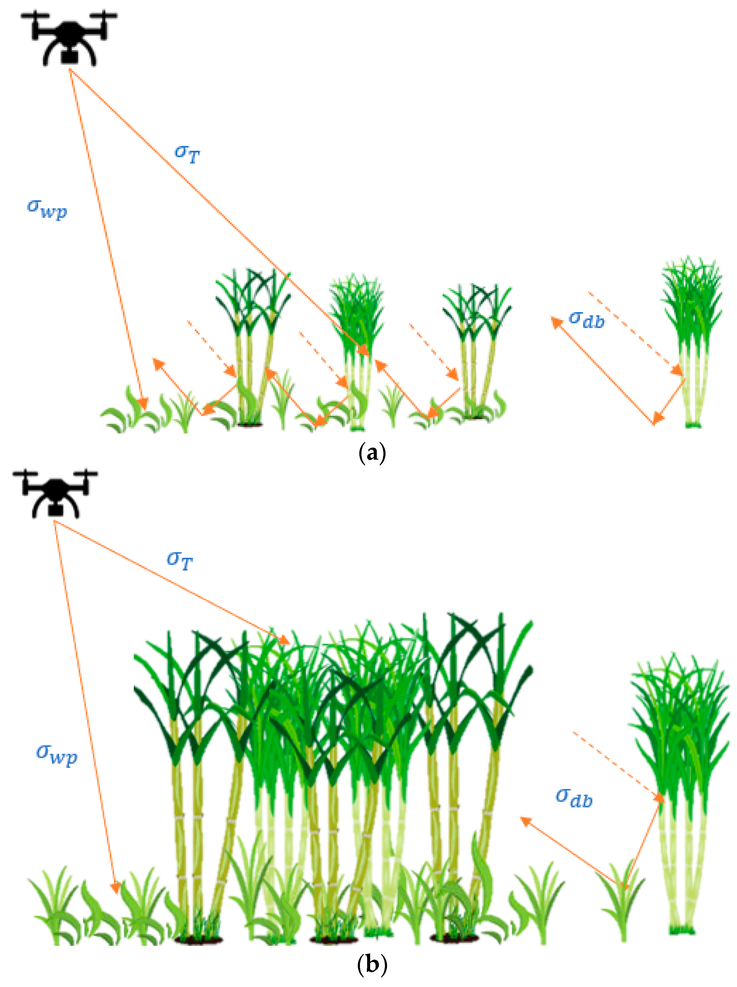
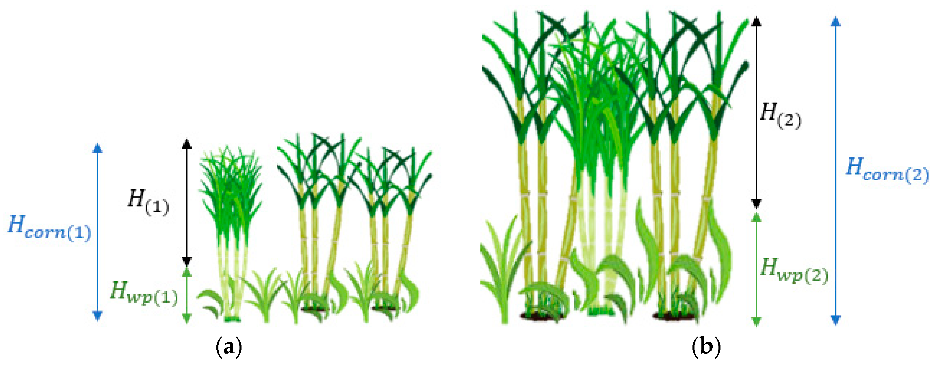
2.4. Estimation Model for Corn Crop Growth

Using the DInSAR model described above to retrieve the height difference from the phase information, and taking into account the reflectivity of the corn crop and the soil with weed plants around it, a model for estimating the growth of a corn crop between two dates is proposed, considering the reflectivity contribution at different development stages of the crop. This model is briefly described in Figure 5.
The reflectivity data obtained from the input images can be decomposed as follows [2]:
σ T = σ c o r n + σ w p + σ d b ,
where σ T is the total reflectivity measured by the radar, σ c o r n represents the corn reflectivity, σ w p is the reflectivity of the soil with weed plants that can be measured in an adjacent area to the corn crop and σ d b is the reflectivity of the double-bounce between the crop stem and the soil, as illustrated in Figure 6. At different stages of the crop growth, the proportions of these reflectivities vary. In early stage growth, shown in Figure 6a, the portion due to double bounce is the most significant, while in late-stage growth, pictured in Figure 6b, the contribution of the corn crop is dominant.
Consider that σ w p can be estimated from the reflectivity of areas close to the crop so that it can be subtracted from Equation (6); thus, the resulting reflectivity, σ R , is as follows:
σ R = σ T σ w p = σ c o r n + σ d b .
Assuming that σ c o r n is proportional to σ R by a contribution factor K R [ 0 , 1 ] , then:
σ c o r n = K R σ R .
Also, the double-bounce contribution can be estimated from K R and σ R as follows:
σ d b = ( 1 K R ) σ R .
As the presence of stems and branches is dominant during the early stages of crop growth, the contribution factor, K R , is negligible and, from Equation (9), σ d b σ R . On the other hand, in late stages of crop growth, the double-bounce contribution decreases drastically due to the presence of leaves; thus, the contribution factor K R 1 and, from Equation (8), σ c o r n σ R .
To calculate the height difference measured between two different days, consider the two different stages of crop growth shown in Figure 7.
Assume that, on Day 1, the height of the crop is H c o r n ( 1 ) , the height of the weed plants is H w p ( 1 ) and the difference between them is H ( 1 ) = H c o r n ( 1 ) H w p ( 1 ) . Similarly, for Day 2, consider that H ( 2 ) = H c o r n ( 2 ) H w p ( 2 ) . Then, the total estimated height variation, Δ H = H ( 2 ) H ( 1 ) , can be calculated as:
Δ H = Δ H c o r n Δ H w p ,
where Δ H c o r n = H c o r n ( 2 ) H c o r n ( 1 ) is the height variation corresponding to the crop and Δ H w p = H w p ( 2 ) H w p ( 1 ) is the height variation due to the growth of weed plants. Equation (10) is only valid when contributions can be measured separately.
The radar measures a sum of complex contributions. The amplitude of the return signal is proportional to σ T , and the interferometric phase is proportional to ΔH, as seen in Equations (3) and (4). As the ratio σ c o r n / σ T approaches unity, Δ H c o r n becomes the major contribution in Equation (10). The same reasoning can be made for σ w p and Δ H w p . In that way, a simple solution is to correct Equation (10) by weighting each contribution by its respective reflectivity.
First, let Equation (7) can be rewritten as follows:
1 = σ c o r n σ T + σ d b σ T + σ w p σ T = K c o r n 2 + K d b 2 + K w p 2 ,
where
K c o r n = σ c o r n σ T = K R σ R σ T ,
K d b = σ d b σ T ,
K w p = σ w p σ T ,
are the corn, weed and double-bounce contributing factors, respectively.
Now, assuming that each contribution can be weighted by its respective contributing factor, the difference in height measure by the radar between two consecutive days can be expressed by the following:
Δ H = Δ H c o r n K c o r n Δ H w p K w p .
Then, from Expressions (12), (14) and (15) comes the following:
Δ H c o r n = 1 K R σ T σ R ( Δ H + Δ H w p   K w p ) .
Next, a new correction factor K = 1 / K R is defined based on field measurement data as follows:
K = Δ H c o r n ( f m ) σ T σ R ( Δ H + Δ H w p K w p ) ,
where Δ H c o r n ( f m ) represents the height difference data measured on the crop. This new correction factor (K) is only valid for the corn model.
Finally, the estimated growth between two dates in a corn crop can be described as follows:
Δ H c o r n - e s t = K σ T σ R ( Δ H T + H w p K w p ) .

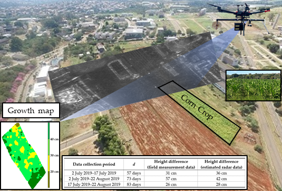
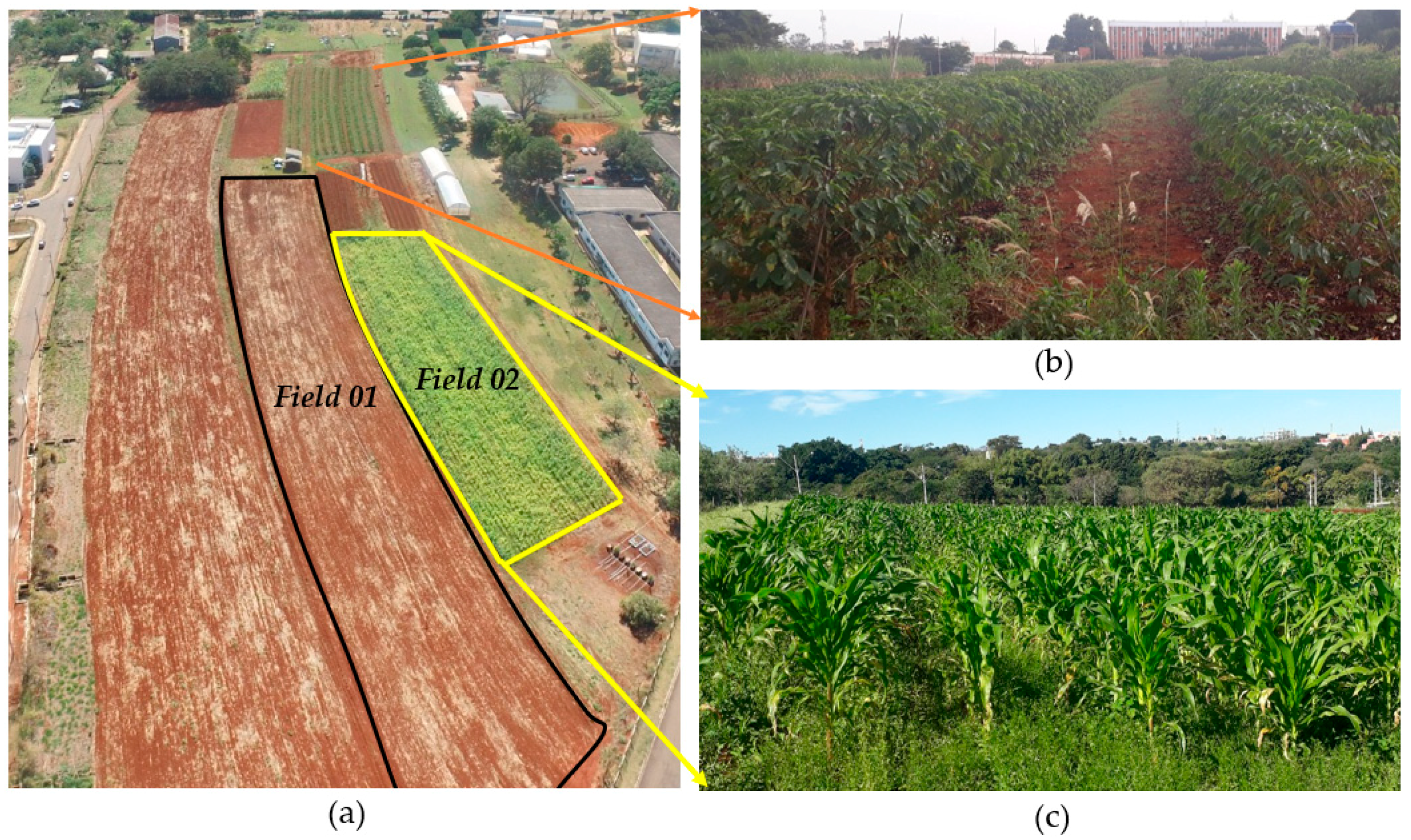
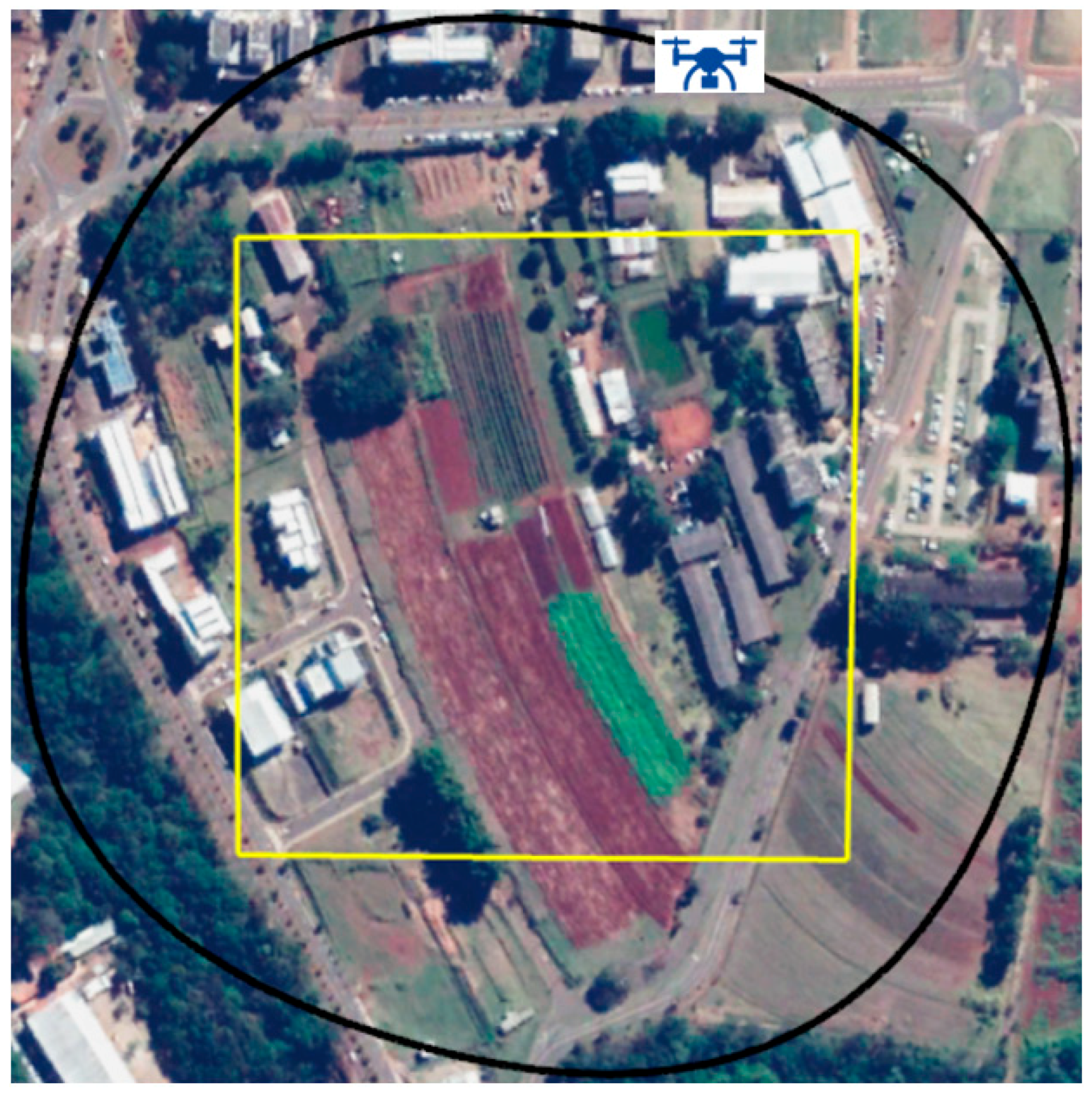
2.5. Experimental Site

The experimental site covers an area of 300 m × 300 m, located at the School of Agricultural Engineering of the University of Campinas (UNICAMP), as shown in Figure 8. The survey flights occurred on the following dates: 11 December 2018; and 17 April, 2 July, 17 July and 22 August 2019.

2.6. Field Measurements

Height measurements of coffee and corn crops, depicted in Figure 8b,c, respectively, were carried out over nine months. In this period, the corn reached the maturity stage in December 2018, and a new crop was set in July 2019. Coffee reached the maturity stage in March 2019. The corn crop is structured with 14 rows, where 20 height measurements were made per row. The heights were measured from the soil to the top of the corn crop. The following measurements were taken on the same days of the flight surveys: 2 July, 17 July and 22 August 2019. The field measurements of the corn crop height are subjected to the natural variability of visual measurement errors.
During the survey period, corn was sown in two areas: field 01 and 02, as shown in Figure 8a. Hereafter, fields 01 and 02 will be labeled as C1 and C2, respectively, where “C” denotes the corn culture.

2.7. Drone-Borne SAR Data Acquisition

Three trihedral corner reflectors with square sides and an edge length of 0.6 m were used as a ground and radiometric calibration reference. The resulting radar cross-section is 20 dBsm.
On each acquisition date, the experiment with the drone-borne system was executed as follows:
  • Mount three corner reflectors on the test site, for planimetric and radiometric calibration purposes;
  • Place the GNSS ground station close to the initial position of the drone and start the GNSS recording;
  • Perform each flight over the experimental site, following the subsequent procedure: turn on the drone and the radar, wait 15 min for simultaneous and stationary recording of ground station and radar GNSS data, take-off, perform the same circular flight track, land, wait 15 min for simultaneous and stationary recording of ground station and radar GNSS data, and turn-off the radar and the drone;
  • Dismount the GNSS ground station and the drone. Download the acquired data for processing.

2.8. Drone-Borne SAR Data Processing

The collected data were processed as follows:
  • Differential GNSS processing of the ground station and the radar GNSS receivers;
  • IMU and differential GNSS data fusion for generating position and antenna orientation history;
  • Radar data processing at each acquisition date, according to Section 2.2: range compression and back-projection for the azimuth compression. The output is a geocoded single-look-complex (SLC) image;
  • Verification of the absolute position of the corner reflectors in the geocoded SLC images;
  • Differential interferometric processing with data from previous acquisitions, as defined in Section 2.3;
  • Production of the crop growth map, as described in Section 2.4;
  • Generation of the corresponding multi-look images with 30 cm × 30 cm sampling.

3. Results

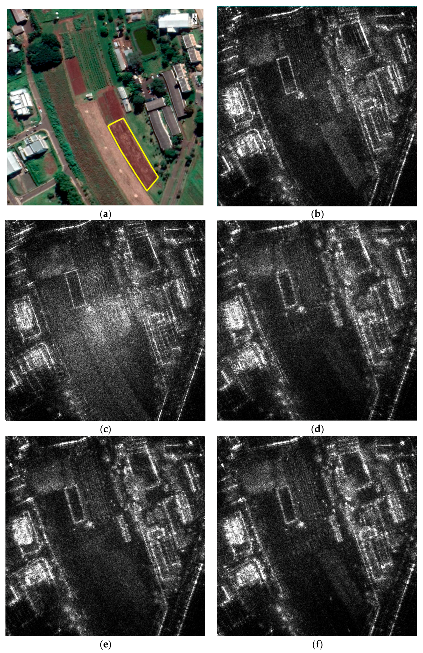
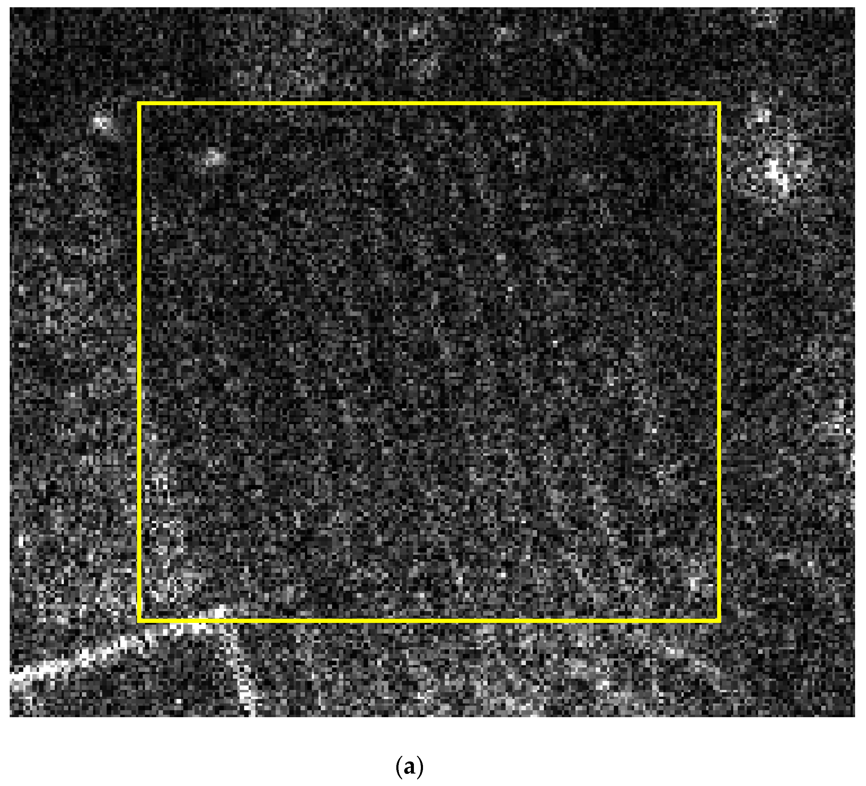
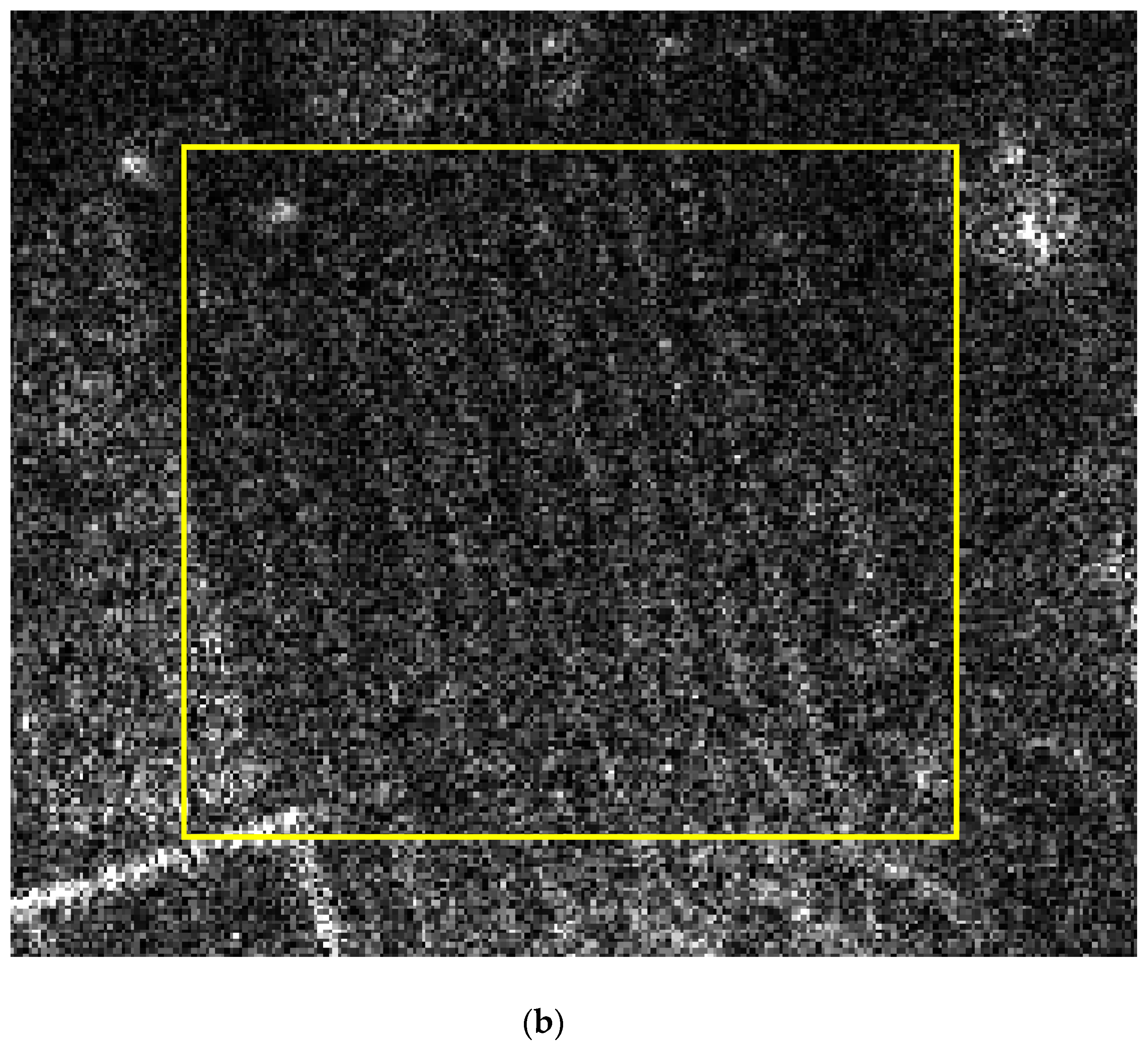
3.1. Drone-Borne SAR Images

The circular flights over the experimental site were carried out by following the path shown in Figure 9. Figure 10 displays the SAR images acquired with circular flights on different acquisition dates. Each image depicts an area of 300 m × 300 m, with 30 cm sampling in both directions.
Figure 10b shows the area C2 with the corn crop in a mature stage. The new seeding of area C2 took place in July 2019, shown in Figure 10d, and this area presents increasing reflectivity through Figure 10e,f, until reaching its maturity.

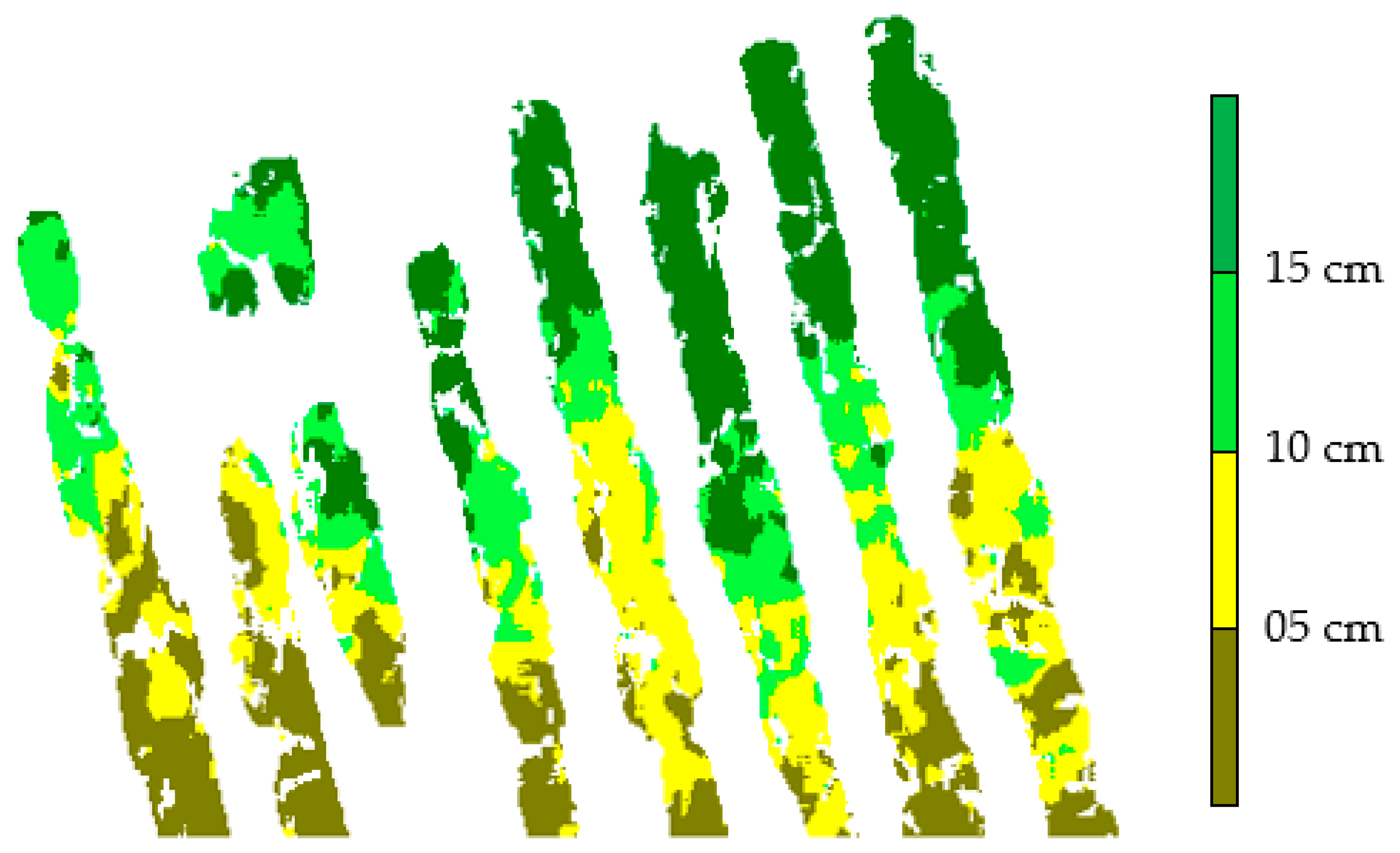
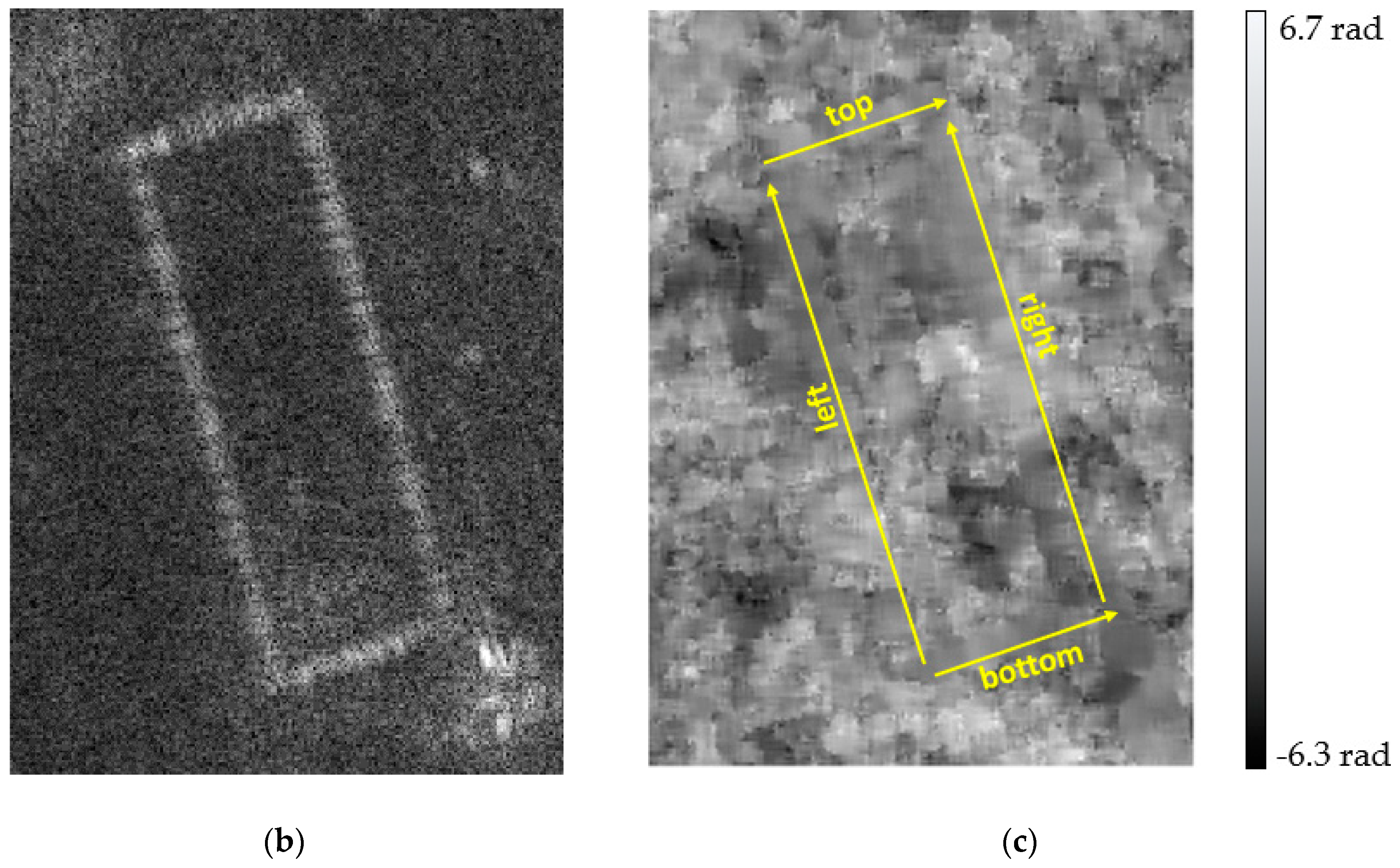
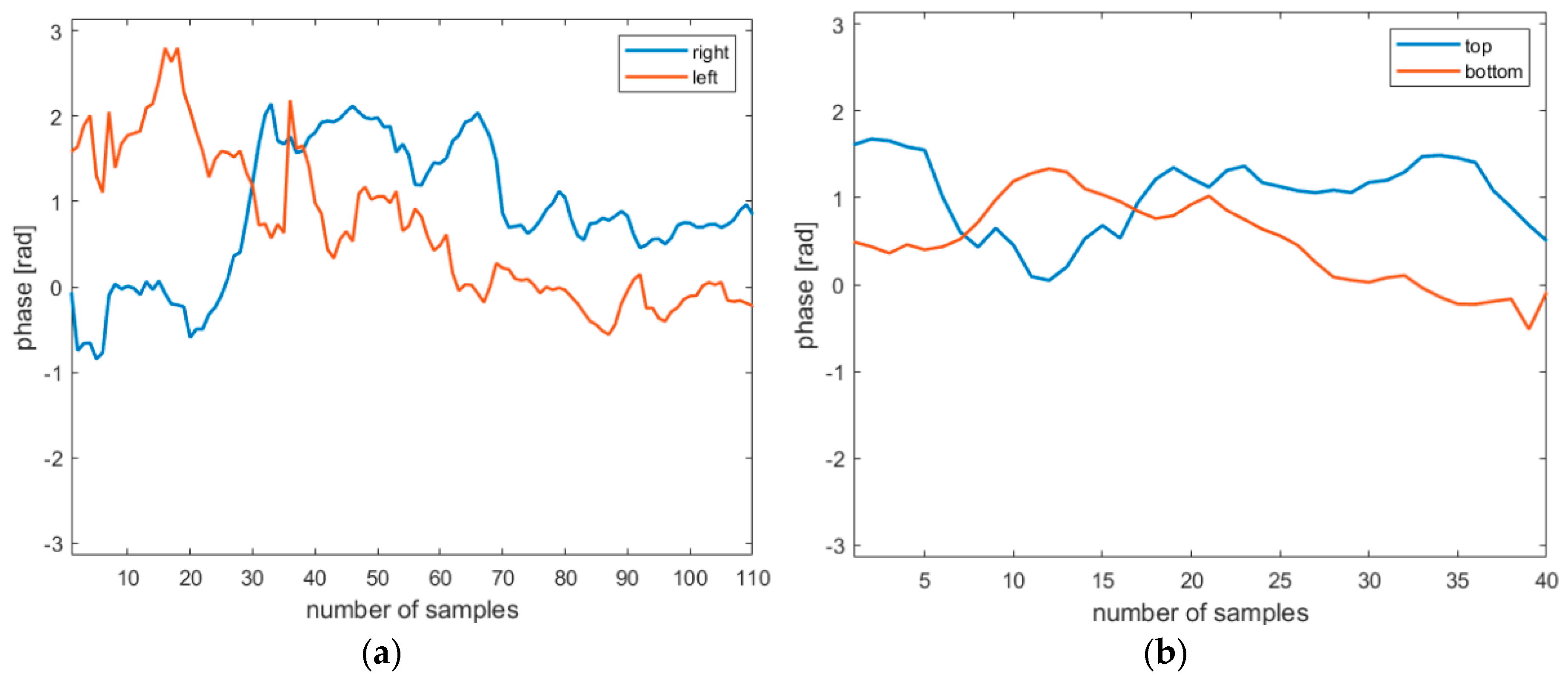
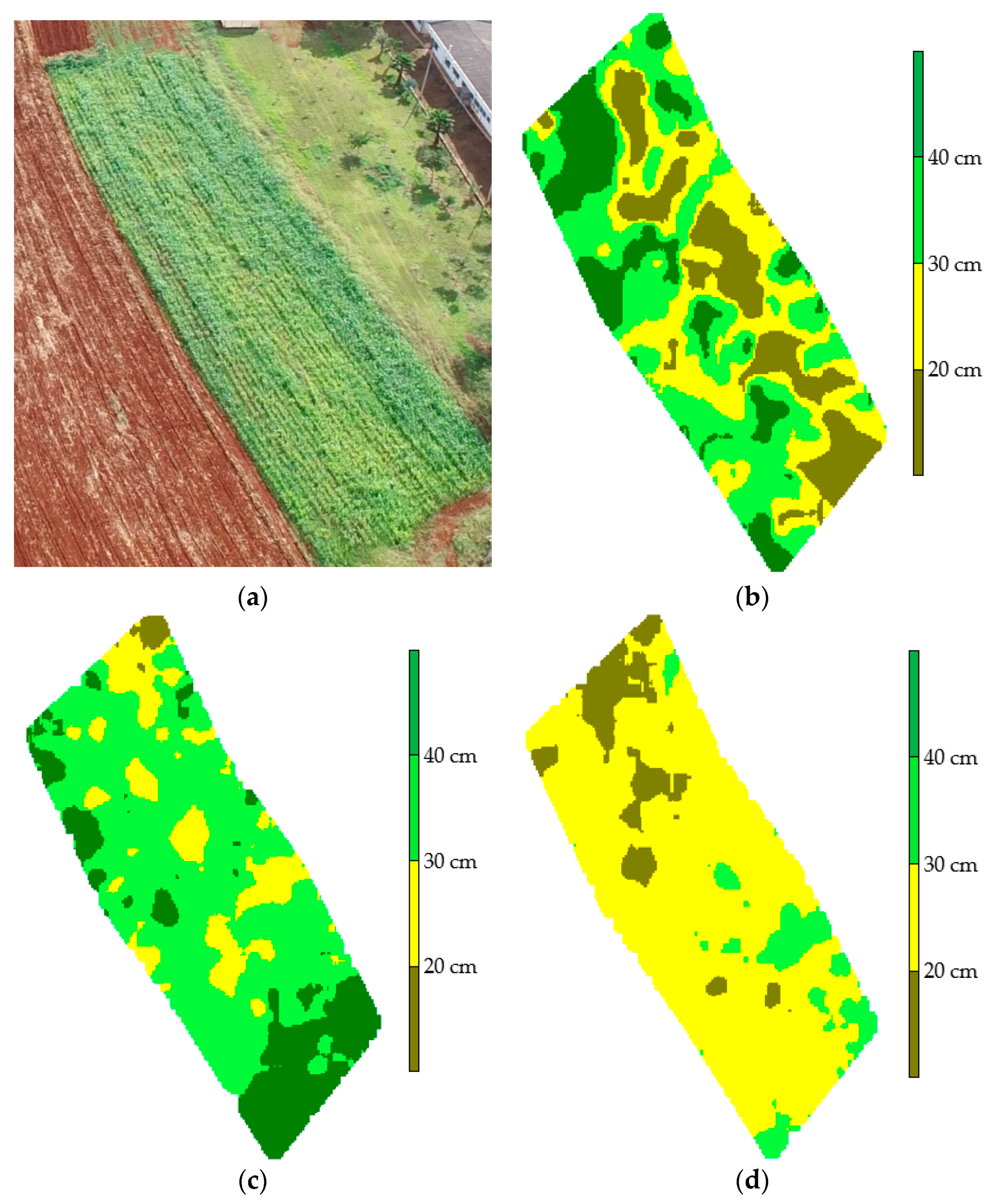
3.2. Qualitative Validation of Growth Deficit Maps

DInSAR technique was applied to the campaigns of 5 December and 11 December 2018, and 17 April 2019, on coffee, sugar cane and corn crops. According to the field data, the corn crop was present only on the first two dates mentioned, and the other crops had an insignificant height variation between the three campaign dates. DInSAR provided a compatible result for these crops, showing a negligible height variation during those dates.
The first trial for a crop growth map was performed with the coffee crop, presented in Figure 8. No field measurement of the crop height variation was determined. However, a rough growth estimate of about 10 cm was expected, as the coffee crop was quite mature in December. Because of a small morphology alteration in the crop due to its maturity, the interferogram had a low but acceptable coherence of 0.2.
A growth map corresponding to a coffee crop of approximately 1700 m2 is shown in Figure 11. The mean height growth between those dates with DInSAR is 11 cm, with a standard deviation of 6 cm. The south area of the coffee crop presented less growth than the north area. A mask was used to discard all targets that do not correspond to the coffee crop. Moreover, a 15 × 15 moving average filter was used over the interferogram, with a pixel spacing of 30 cm × 30 cm. Only data with a coherence greater than 0.1 were considered valid data. This result has motivated a more in-depth study of DInSAR for growth maps.
Figure 12 shows the corresponding SAR images for the acquisition dates of 11 December 2018, and 17 April 2019, where the yellow squares represent the coffee crop for which the growth map of Figure 11 was produced.

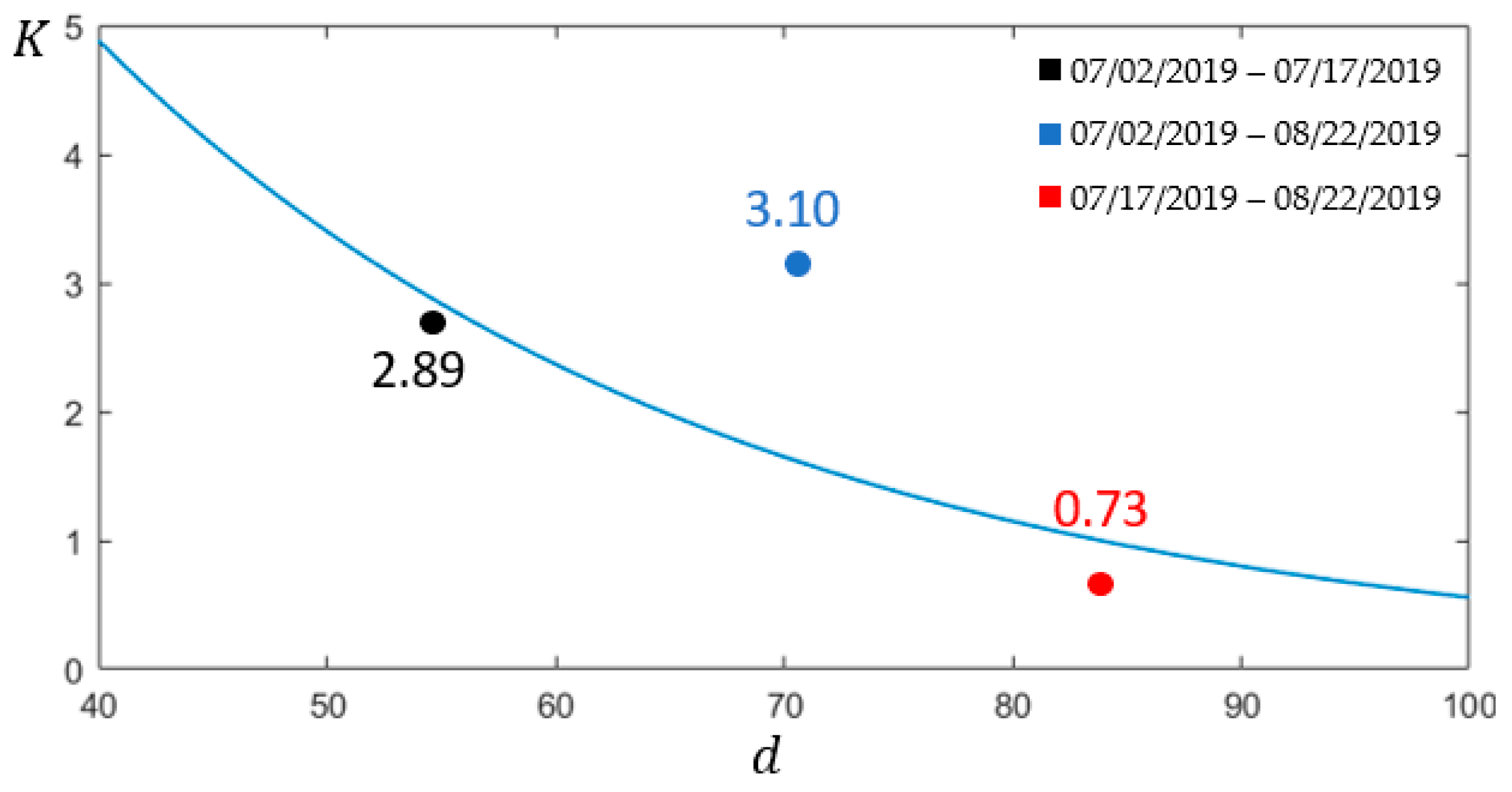
3.3. Quantitative Validation of Growth Deficit Maps

SLC images of circular flight tracks were used to validate the growth estimation model considering the reflectivity contribution. The high resolution allows a much easier analysis, as the cornfield C2 is rather small.
To obtain the phase reference, known as the zero-movement phase, an object that would remain static during all flights was searched. Initially, it was thought to use the dihedral corner reflectors. However, it would not be possible to leave the dihedral corner reflectors at all times in the study area, because other daily activities are carried out there. Besides, a dihedral corner reflector can only be observed during a small portion of the circular track. Therefore, a metal fence near the crop area was chosen as a reference, as it is a fixed object and can be observed during the entire flight (see Figure 13).
To obtain the zero-movement phase, profiles were drawn for the interferogram over the area corresponding to the metal fence, Figure 13c. The profiles are shown in Figure 14a,b. The zero-movement phase was calculated by using the average of the profiles, which, in this example, resulted in 0.76 rad.
Then, the height growth of the cornfield C2 was monitored, as shown in Table 2. These data, together with the reflectivity data for the corn crop and a neighboring area (see Figure 6), were used to estimate the correction factor, K, of Equation (17), which varies along with the phenological life of the corn crop.
Figure 15 displays three values for the correction factor, K, estimated by using the available radar data and field measurement data from the three different periods presented in Table 2. Figure 15 also shows the fitted curve (blue line) for the correction factor, K, as a function of the corn phenology stage.
Due to the small amount of data, there is some flexibility when choosing the type of equation that best fits the experimental data. An exponential fitting curve was chosen, and the resultant expression is as follows:
K = 20.75 exp ( 0.03617 d ) ,
where d represents the average number of days after planting, calculated over each data collection period, as displayed in Table 3. Equation (19) is a first attempt to find an expression for K, using the few available data, and it is calculated with MATLAB Curve Fitting Toolbox [19].
Table 3 also shows the height-difference data between two dates obtained by field measurements in the corn crop and estimates from the proposed model, using the radar data together with the correction factor, K.
Figure 16 presents the crop growth maps derived from the same acquisition intervals displayed in Figure 15. Rapid growth can be seen from 2 July to 17 July, though growth is noticeably slower between 17 July and 22 August.

4. Discussion

Determining the zero-movement phase is an essential step for estimating crop growth. The zero-movement phase is not null due to external factors such as the system’s thermal noise, the difference between flight paths from distinct dates and internal changes of the radar system between different flights [16]. The chosen reference object was a metal fence because it is always fixed, thus providing more robust results than moving objects, for which precise positioning between separate flights is not guaranteed. Moreover, it can be seen from all directions in a circular flight track, and it is typically found near crop fields.
Corner reflectors are not practical reference points for DInSAR, as they should be well fixed and kept clean during the DInSAR observation period. The authors intend to continue using corner reflectors, only for purposes of planimetric accuracy and height calibration. Luneburg lenses could also be used to better calibrate the back-projection processor [20].
No other publications were found that use the DInSAR technique on a corn crop to estimate growth, but some similar works are noteworthy. Erten et al. [10] used the DInSAR technique, with the TANDEM-X satellite, over a rice cultivation area, and were able to estimate growth with an RMSE of 18 cm. Cao et al. [21] used an airborne L-band radar system to measure landslide with a precision of a few centimeters.
In this work, a first attempt to monitor growth was carried out with a coffee crop, as described in Section 3.2. The coffee had a barely noticeable height variation between 11 December 2018, and 17 April 2019. However, using DInSAR, it was possible to measure an 11 cm growth, with a standard deviation of 6 cm. No model will estimate the growth of a crop that hardly grows.
As for the corn crop growth using correction factor K, the errors obtained from 2 July to 17 July 2019, and from 17 July to 22 August 2019, were 5 cm and 2 cm, respectively, while from 2 July to 22 August 2019, the error was 15 cm. Therefore, the longest period between data acquisitions produces the largest error, whereas shorter acquisition periods provide more accurate results. Therefore, to achieve a more accurate growth model oriented to the corn crop, it is necessary to retrieve a better estimation of the variable K, and thus more flights are required. Another way to develop this model would be to use the two interferometric C-band antennas to estimate crop height [22].
The corn crop was chosen due to its rapid growth. Nevertheless, this work could be extended to other crops, such as sugar cane or coffee. The case of sugar cane, which grows slower than corn, is of particular interest to the authors; therefore, more campaigns will be needed over time.

5. Conclusions

This work proposes a novel method for estimating the growth of different crops by executing circular flight paths with a drone-borne DInSAR operating in the L-band with HH polarization. First tests on late-stage coffee, corn and sugar cane crops have shown that it is possible to reliably estimate small height variations. In the case of coffee, the growth within approximately four months was estimated at 11 cm, with a standard deviation of 6 cm. Such a growth rate is difficult to perceive visually or to measure with conventional tools.
Furthermore, a method is proposed to estimate the growth of a corn crop, taking into account its phenological development. Although more campaigns on the area of interest are still necessary, these first-stage results show a strong agreement with the measured field data. The largest error was 15 cm, corresponding to the longest period between data acquisitions, for which the crop growth was approximately 55 cm. In contrast, errors of up to 5 cm were obtained for shorter acquisition periods.
The images obtained from the circular flights were processed with the back-projection algorithm using a 30 cm × 30 cm sampling. In future work, a more accurate growth estimation is expected since back-projection images shall be processed with a 5 cm × 5 cm sampling.
The authors are motivated to continue with this line of research, taking as a starting point the methods and first-stage results obtained so far. More consistent results are expected in the near future, when more data will be available.

Author Contributions

Conceptualization, G.O. and H.E.H.-F.; investigation, methodology, software and validation, G.O., M.S.A., J.A.G., V.C., L.S.B. and F.C.; validation, J.Y. and D.L.; formal analysis and writing, G.O., M.S.A., J.A.G., L.P.O., V.C., F.C. and L.F.M.; supervision, review and funding acquisition, L.P.O., B.T., D.L., L.H.G. and H.E.H.-F. All authors have read and agreed to the published version of the manuscript.

Funding

This research was funded by government agencies CAPES and CNPq and the São Paulo State agency FAPESP, under the contracts PITE 2017/19416-3 and PIPE 2018/00601-8.

Acknowledgments

We thank the teams of the schools of Electrical and Computer Engineering and of Agricultural Engineering of the University of Campinas, UNICAMP, for the given support.

Conflicts of Interest

The authors declare no conflicts of interest.

References

  1. Liu, C.-A.; Chen, Z.-X.; Shao, Y.; Chen, J.-S.; Hasi, T.; Pan, H.-Z. Research advances of SAR remote sensing for agriculture applications: A review. J. Integr. Agric. 2019, 18, 506–525. [Google Scholar] [CrossRef] [Green Version]
  2. Lin, H.; Chen, J.; Pei, Z.; Zhang, S.; Hu, X. Monitoring Sugarcane Growth Using ENVISAT ASAR Data. IEEE Trans. Geosci. Remote Sens. 2009, 47, 2572–2580. [Google Scholar] [CrossRef]
  3. Baghdadi, N.; Cresson, R.; Todoroff, P.; Moinet, S. Multitemporal Observations of Sugarcane by TerraSAR-X images. Sensors 2010, 10, 8899–8919. [Google Scholar] [CrossRef] [PubMed] [Green Version]
  4. Skriver, H. Crop Classification by Multitemporal C- and L-Band Single- and Dual-Polarization and Fully Polarimetric SAR. IEEE Trans. Geosci. Remote Sens. 2012, 50, 2138–2149. [Google Scholar] [CrossRef]
  5. Liu, X.; Jiao, L.; Tang, X.; Sun, Q.; Zhang, D. Polarimetric Convolutional Network for PolSAR Image Classification. IEEE Trans. Geosci. Remote Sens. 2019, 57, 3040–3054. [Google Scholar] [CrossRef] [Green Version]
  6. Lin, K.-F.; Perissin, D. Single-Polarized SAR Classification Based on a Multi-Temporal Image Stack. Remote Sens. 2018, 10, 1087. [Google Scholar] [CrossRef] [Green Version]
  7. Intarat, T.; Rakwatin, P.; Srestasathien, P.; Triwong, P.; Tangsiriworakul, C.; Noivum, S. Potential of Sugar cane monitoring using Synthetic Aperture Radar in Central Thailand. In Proceedings of the 36th Asian Conference of Remote Sensing, Quezon City, Philippines, 19–23 October 2015. [Google Scholar]
  8. Rossi, C.; Erten, E. Paddy Rice Monitoring Using TanDEM-X. IEEE Trans. Geosci. Remote Sens. 2015, 53, 900–910. [Google Scholar] [CrossRef] [Green Version]
  9. Wang, H.; Magagi, R.; Goita, K. Polarimetric Decomposition for Monitoring Crop Growth Status. IEEE Geosci. Remote Sens. Lett. 2016, 13, 870–874. [Google Scholar] [CrossRef]
  10. Erten, E.; Lopez-Sanchez, J.; Yuzugullu, O.; Hajnsek, I. Retrieval of agricultural crop height from space: A comparison of SAR techniques. Remote Sens. Environ. 2016, 187, 130–144. [Google Scholar] [CrossRef] [Green Version]
  11. Frey, O.; Werner, C.L.; Coscione, R. Car-borne and UAV-borne mobile mapping of surface displacements with a compact repeat-pass interferometric SAR system at L-band. In Proceedings of the IGARSS 2019—2019 IEEE International Geoscience and Remote Sensing Symposium, Yokohama, Japan, 28 July–2 August 2019; pp. 274–277. [Google Scholar]
  12. Moreira, L.; Castro, F.; Góes, J.A.; Bins, L.; Teruel, B.; Fracarolli, J.; Castro, V.; Alcântara, M.; Oré, G.; Luebeck, D.; et al. A Drone-borne Multiband DInSAR and Applications. In Proceedings of the 2019 IEEE Radar Conference (RadarConf), Boston, MA, USA, 22–26 April 2019; pp. 1–6. [Google Scholar]
  13. Ishimaru, A.; Chan, T.-K.; Kuga, Y. An imaging technique using confocal circular synthetic aperture radar. IEEE Trans. Geosci. Remote Sens. 1998, 36, 1524–1530. [Google Scholar] [CrossRef]
  14. Palm, S.; Sommer, R.; Pohl, N.; Stilla, U. Airborne SAR on Circular Trajectories to Reduce Layover and Shadow Effects of Urban Scenes; International Society for Optics and Photonics: Edinburgh, UK, 2016; p. 100080N. [Google Scholar]
  15. Doerry, A.W.; Bishop, E.E.; Miller, J.A. Basics of Backprojection Algorithm for Processing Synthetic Aperture Radar Images; Sandia National Laboratories: Albuquerque, NM, USA, 2016; pp. 1–57.
  16. Richards, J.A. Remote Sensing with Imaging Radar; Signals and Communication Technology; Springer: Heidelberg, Germany, 2009; ISBN 9783642020193. [Google Scholar]
  17. Hanssen, R.F. Radar Interferometry Data Interpretation and Error Analysis; Remote Sensing and Digital Image Processing; Kluwer Academic: Dordrecht, The Netherlands, 2001; ISBN 9780792369455. [Google Scholar]
  18. Giglia, D.C.; Romero, L.A. Robust two-dimensional weighted and unweighted phase unwrapping that uses fast transforms and iterative methods. J. Opt. Soc. Am. 1994, 11, 107–117. [Google Scholar] [CrossRef]
  19. Curve Fitting Toolbox; The Math Works: Natick, MA, USA, 2018.
  20. Ponce, O.; Prats-Iraola, P.; Scheiber, R.; Reigber, A.; Moreira, A. First Airborne Demonstration of Holographic SAR Tomography with Fully Polarimetric Multicircular Acquisitions at L-Band. IEEE Trans. Geosci. Remote Sens. 2016, 54, 6170–6196. [Google Scholar] [CrossRef]
  21. Cao, N.; Lee, H.; Zaugg, E.; Shrestha, R.; Carter, W.; Glennie, C.; Wang, G.; Lu, Z.; Fernandez-Diaz, J.C. Airborne DInSAR Results Using Time-Domain Backprojection Algorithm: A Case Study Over the Slumgullion Landslide in Colorado With Validation Using Spaceborne SAR, Airborne LiDAR, and Ground-Based Observations. IEEE J. Sel. Top. Appl. Earth Obs. Remote Sens. 2017, 10, 4987–5000. [Google Scholar] [CrossRef]
  22. Duerch, M. Backprojection for Synthetic Aperture Radar. Ph.D. Thesis, Brigham Young University, Provo, UT, USA, 2013. [Google Scholar]
Figure 1. Image of the drone-borne SAR with the L-band, the P-band and the two C-band antennas.
Remotesensing 12 00615 g001
Figure 2. DInSAR circular flight pattern and illumination geometry.
Remotesensing 12 00615 g002
Figure 3. Interaction between radar signal and crop height.
Remotesensing 12 00615 g003
Figure 4. Block diagram for DInSAR processing.
Remotesensing 12 00615 g004
Figure 5. Block diagram for the estimation model for corn crop growth.
Remotesensing 12 00615 g005
Figure 6. Representation of reflectivity in the corn crop at different growth stages. (a) Early stage growth. (b) Late-stage growth.
Remotesensing 12 00615 g006
Figure 7. Crop in two different stages. (a) Day 1. (b) Day 2.
Remotesensing 12 00615 g007
Figure 8. Overview of the experimental site at UNICAMP. (a) Aerial View with fields 01 and 02 at the bottom and the coffee crop at the top, on 22 August 2019. Field 01 was bare. (b) Ground photo of the coffee crop. (c) Ground photo of the corn crop on field 02.
Remotesensing 12 00615 g008
Figure 9. Description of the circular flight. In black, the circular flight track, and in yellow, the study area of 300 m × 300 m.
Remotesensing 12 00615 g009
Figure 10. Temporal comparison between (a) optical image from Google Earth and drone-borne SAR images of the circular flight tracks, acquired on (b) 11 December 2018; (c) 17 April 2019; (d) 2 July 2019; (e) 17 July 2019; and (f) 22 August 2019. Field C2 has a yellow border in (a).
Remotesensing 12 00615 g010
Figure 11. Growth map of the coffee crop from 11 December 2018, to 17 April 2019.
Remotesensing 12 00615 g011
Figure 12. SAR images of coffee crop acquired on (a) 11 December 2018; and (b) 17 April 2019.
Remotesensing 12 00615 g012aRemotesensing 12 00615 g012b
Figure 13. (a) Optical image of the metal fence; (b) radar image of the metal fence; and (c) unwrapped interferogram corresponding to the metal fence.
Remotesensing 12 00615 g013aRemotesensing 12 00615 g013b
Figure 14. (a) Right and left side profiles of the fence phase; (b) top and bottom side profiles of the fence phase.
Remotesensing 12 00615 g014
Figure 15. Correction factor (K) as a function of the corn phenology stage.
Remotesensing 12 00615 g015
Figure 16. Crop growth maps derived from three acquisition intervals: (a) optical reference image from corn crop (b) from 2 July to 17 July 2019; (c) from 2 July to 22 August 2019; and (d) from 17 July to 22 August 2019.
Remotesensing 12 00615 g016
Table 1. Main parameters of radar acquisition.
Radar ParametersValue
Carrier wavelength22.84 cm
Bandwidth150 MHz
PolarizationHH
Peak Power100 mW
Mean Power1 mW
Pulse Repetition Frequency10 kHz
Incidence angle45 deg
Mean drone height120 m
Mean drone velocity2 m/s
Maximum acquisition time20 min
Motion Sensing System, MSSD-GNSS + IMU
DInSAR accuracy6 mm
Range resolution1 m
Azimuth resolution10 cm
Processed azimuth bandwidth20 Hz
Processed aperture at 45 deg. incidence angle196 m
Single-look-complex range sampling61 cm
Single-look-complex azimuth sampling5 cm
Table 2. Corn crop field measurements.
Height Measurement DateDays after PlantingCorn Height
2 July 20194868 cm
17 July 20196799 cm
22 August 201999125 cm
Table 3. Comparison between field measurement data and estimated radar data in the corn crop for height difference information.
Data Collection PerioddHeight Difference
(Field Measurement Data)
Height Difference (Estimated Radar Data)
2 July 2019–17 July 201957 days31 cm36 cm
2 July 2019–22 August 201973 days57 cm42 cm
17 July 2019–22 August 201983 days26 cm28 cm

