Article

Evaluation of Seven Atmospheric Profiles from Reanalysis and Satellite-Derived Products: Implication for Single-Channel Land Surface Temperature Retrieval

1
School of Environment and Resources, Shanxi University, Taiyuan 030006, China
2
Key Laboratory of Agricultural Remote Sensing, Ministry of Agriculture/Institute of Agricultural Resources and Regional Planning, Chinese Academy of Agricultural Sciences, Beijing 100081, China
3
Anhui Province Key Laboratory of Wetland Ecosystem Protection and Restoration, Anhui University, Hefei 230601, China
4
College of Resources and Environment, University of Chinese Academy of Sciences, Beijing 100049, China
*
Author to whom correspondence should be addressed.
Submission received: 30 January 2020 / Revised: 25 February 2020 / Accepted: 28 February 2020 / Published: 1 March 2020

Abstract

:
Land surface temperature (LST) is vital for studies of hydrology, ecology, climatology, and environmental monitoring. The radiative-transfer-equation-based single-channel algorithm, in conjunction with the atmospheric profile, is regarded as the most suitable one with which to produce long-term time series LST products from Landsat thermal infrared (TIR) data. In this study, the performances of seven atmospheric profiles from different sources (the MODerate-resolution Imaging Spectroradiomete atmospheric profile product (MYD07), the Atmospheric Infrared Sounder atmospheric profile product (AIRS), the European Centre for Medium-range Weather Forecasts (ECMWF), the Modern-Era Retrospective analysis for Research and Applications, Version 2 (MERRA2), the National Centers for Environmental Prediction (NCEP)/Global Forecasting System (GFS), NCEP/Final Operational Global Analysis (FNL), and NCEP/Department of Energy (DOE)) were comprehensively evaluated in the single-channel algorithm for LST retrieval from Landsat 8 TIR data. Results showed that when compared with the radio sounding profile downloaded from the University of Wyoming (UWYO), the worst accuracies of atmospheric parameters were obtained for the MYD07 profile. Furthermore, the root-mean-square error (RMSE) values (approximately 0.5 K) of the retrieved LST when using the ECMWF, MERRA2, NCEP/GFS, and NCEP/FNL profiles were smaller than those but greater than 0.8 K when the MYD07, AIRS, and NCEP/DOE profiles were used. Compared with the in situ LST measurements that were collected at the Hailar, Urad Front Banner, and Wuhai sites, the RMSE values of the LST that were retrieved by using the ECMWF, MERRA2, NCEP/GFS, and NCEP/FNL profiles were approximately 1.0 K. The largest discrepancy between the retrieved and in situ LST was obtained for the NCEP/DOE profile, with an RMSE value of approximately 1.5 K. The results reveal that the ECMWF, MERRA2, NCEP/GFS, and NCEP/FNL profiles have great potential to perform accurate atmospheric correction and generate long-term time series LST products from Landsat TIR data by using a single-channel algorithm.

Graphical Abstract

1. Introduction

Land surface temperature (LST) is a key parameter that reflects the physical processes of land at local and global scales, and it plays an important role in the interaction between the surface and the atmosphere, as well as the process of water cycle and energy exchange [1,2,3,4]. It is of great significance to the studies of hydrology, ecology, environment, and biogeochemistry [5,6,7]. Satellites carrying thermal infrared (TIR) sensors can effectively measure LST at the local and global scales [8,9,10,11].
Landsat satellites carrying TIR sensors have been launched since the 1980s. Table 1 summarizes the characteristics of the TIR sensors onboard the Landsat satellites. Except for the Thermal Infrared Sensor (TIRS), which is aboard the Landsat 8 satellite, other sensors (e.g., the Thematic Mapper (TM) and the Enhanced Thematic Mapper (ETM+)) have only one TIR band [12]. Though TIRS provides satellite measurements at its TIR bands, i.e., bands 10 (10.60–11.19 μm) and 11 (11.50–2.51 μm), the stray light phenomenon causes a severe problem in radiometric calibration in TIRS band 11 [13,14]. Thus, a single-channel algorithm is usually used to estimate LST from TIRS band 10 data [12,15,16,17]. Several single-channel algorithms, including the Qin single-channel algorithm [18,19], the Jimenez-Munoz and Sobrino (JMS) single-channel algorithm [20,21,22], and the radiative transfer equation (RTE)-based single-channel algorithm [23,24] have been proposed in other studies. The RTE-based single-channel algorithm in conjunction with atmospheric profiles has been proven to have high LST retrieval accuracy [25,26].
Atmospheric profiles, in combination with the radiative transfer model (RTM), are crucial for the compensation of the attenuation that is introduced by the atmosphere in the TIR region. With the rapid development of four-dimensional assimilation techniques, several reanalysis atmospheric profile products have been produced by assimilating different radiosonde, ground, and satellite measurements. In addition, some satellite-derived atmospheric and radio sounding profiles are available for the scientific community. The three types of atmospheric profiles have their advantages and disadvantages. A radio sounding profile can characterize atmospheric situations at specific latitudes and longitudes with a high precision. However, it is only available at limited sites and times. Satellite-derived profiles (e.g., the MODerate-resolution Imaging Spectroradiomete (MxD07) and the Atmospheric Infrared Sounder atmospheric profile product (AIRS)) are available at the satellite pixel scale with a relatively high spatial resolution (dozens of kilometers) but only at the satellite overpassing time. Furthermore, satellite-derived profiles may be missed because of the influence of clouds or the problem of the profile retrieval method. Reanalysis profiles are provided at low spatial resolution of several degrees every three or six hours [27]. Nevertheless, they have been provided with spatial continuity since the 1970s.
The RTE-based single-channel algorithm, in conjunction with atmospheric profiles, has great potential to generate long-term time series LST products from Landsat TIR data. Several studies have been carried out to evaluate the performance of satellite-derived or reanalysis profiles in LST retrieval that use single-channel algorithms [28,29,30]. However, only two-to-four atmospheric profiles have been analyzed at limited test sites [31,32,33]. It is still necessary to perform an in-depth analysis and comprehensive comparison of reanalysis and satellite-derived atmospheric profiles in the single-channel LST retrieval algorithm. In this research, seven atmospheric profiles that were derived from multiple sources are compared: two satellite-derived profiles and five reanalysis profiles.

2. Materials and Methods
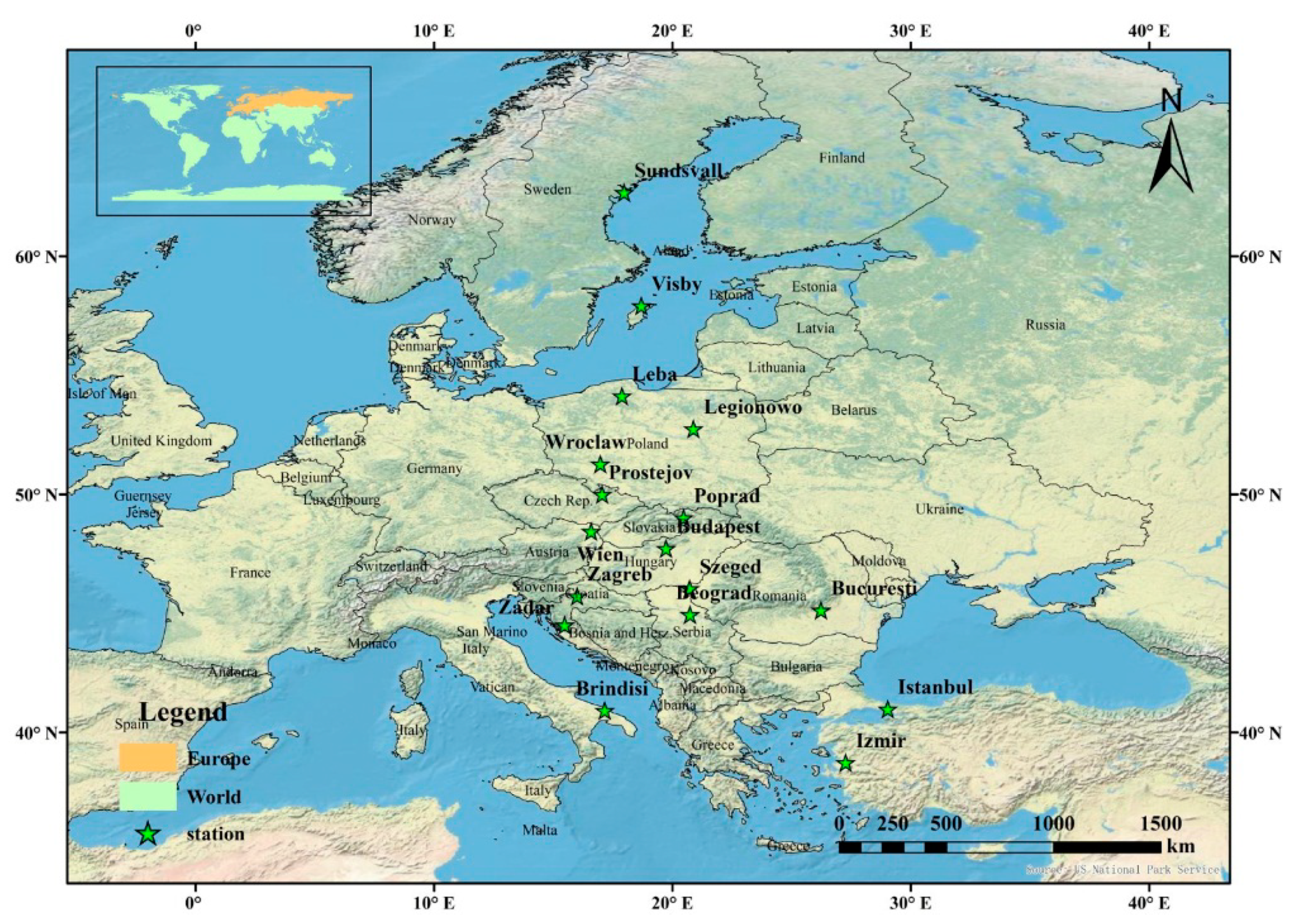
2.1. Data

2.1.1. Atmospheric Profiles

Eight atmospheric profiles that were obtained from multiple sources were used in this study, including one radio sounding profile downloaded from the University of Wyoming (UWYO), two satellite-derived profiles (MxD07 and AIRS), and five reanalysis profiles (the European Centre for Medium-range Weather Forecasts (ECMWF), the Modern-Era Retrospective analysis for Research and Applications, Version 2 (MERRA2), the National Centers for Environmental Prediction (NCEP)/Global Forecasting System (GFS ), NCEP/Final Operational Global Analysis (FNL), and NCEP/Department of Energy (DOE)). The UWYO profile is more representative of real atmospheric situations; therefore, it was used as reference data to evaluate the accuracies of the other seven profiles. Table 2 lists the main characteristics of these atmospheric profiles.
(1). Radio sounding profile
The radio sounding profile (hereafter, the “UWYO profile”) collected by the globally distributed radiosonde stations that was used in this study is from the University of Wyoming and can be downloaded from the website shown in Table 2. The UWYO profile is released twice per day at 0 and 12 UTC. It provides atmospheric pressure, altitude, temperature, relative humidity, dew point temperature, and other parameters.
To ensure that the UWYO profile represents real atmospheric situations at the satellite overpassing time, the time difference between the UWYO profile and the satellite-derived profiles (i.e., MYD07 and AIRS) is limited to 1 h. This study used 17 UWYO radiosonde stations with longitudes ranging from 15° E to 30° E. Figure 1 shows the geolocation of these 17 selected radiosonde stations. Table 3 summarizes the detailed information about these radiosonde stations.
(2). MxD07 profile
The Moderate-resolution Imaging Spectroradiometer (MODIS) instruments are aboard two National Aeronautics and Space Administration (NASA) satellites, i.e., Terra and Aqua, which were sent into orbit on 18 December 1999 and 4 May 2002, respectively. The Terra satellite passes through the equator from north to south at approximately 10:30 am at local solar time. The Aqua satellite passes through the equator in the opposite direction from south to north at approximately 1:30 p.m. [34].
The MODIS atmospheric profile product (MOD07_L2 and MYD07_L2) can be obtained freely from the NASA’s Level-1 and Atmosphere Archive and Distribution System (LAADS) website (https://ladsweb.modaps.eosdis.nasa.gov/). This product provides atmospheric parameters that contain temperature and moisture profiles, atmospheric stability, atmospheric water vapor, and total-ozone burden at a spatial resolution of 5 km. The temperature and water vapor profiles are produced at 20 vertical levels: 1000, 950, 920, 850, 780, 700, 620, 500, 400, 300, 250, 200, 150, 100, 70, 50, 30, 20, 10, and 5 hPa.
(3). AIRS profile
AIRS is another sensor aboard the Aqua satellite. The AIRS L3 daily gridded standard retrieval product (AIRS_3STD) with a spatial resolution of 1° × 1° was used in this study. The temperature profile is reported at 24 pressure levels: 1000, 925, 850, 700, 600, 500, 400, 300, 250, 200, 150, 100, 70, 50, 30, 20, 15, 10, 7, 5, 3, 2, 1.5, and 1 hPa. A water vapor profile is only provided with the first 12 pressure levels [35].
(4). ECMWF profile
The ECMWF Interim Reanalysis (ERA-Interim) is a reanalysis product of the atmosphere that is provided by ECMWF. The ECMWF profile with a spatial resolution of 0.125° × 0.125° was used in this study. It gives geopotential height, pressure, temperature, and relative humidity from the surface up to 1 hPa at 37 vertical levels: 1000, 975, 950, 925, 900, 875, 850, 825, 800, 775, 750, 700, 650, 600, 550, 500, 450, 400, 350, 300, 250, 225, 200, 175, 150, 125, 100, 70, 50, 30, 20, 10, 7, 5, 3, 2, and 1 hPa [36]. It is noted that this profile was not released after 31 August 2019, and it has been replaced by ERA5 reanalysis. However, at the time of our study, the ERA5 profile was not released, so this study used ERA-interim instead of ERA5.
(5). MERRA2 profile
MERRA2 is a NASA atmospheric reanalysis that is generated using the Goddard Earth Observing System Model, Version 5 (GEOS-5) combined with its Atmospheric Data Assimilation System (ADAS), version 5.12.4 [37]. It provides 42 pressure levels at 1000, 975, 950, 925, 900, 875, 850, 825, 800, 775, 750, 725, 700, 650, 600, 550, 500, 450, 400, 350, 300, 250, 200, 150, 100, 70, 50, 40, 30, 20, 10, 7, 5, 4, 3, 2, 1, 0.7, 0.5, 0.4, 0.3, and 0.1 hPa every 6 h with a spatial resolution of 0.625° longitude × 0.5° latitude. Temperature, relative humidity, and geopotential height variables were extracted from the MERRA2 profile.
(6). NCEP/GFS profile
The GFS is a weather forecast model that is produced by the National Centers for Environmental Prediction (NCEP). The spatial resolution is 0.5° × 0.5° and 1° × 1°, and the temporal resolution is 6 h at 00, 06, 12, and 18 UTC daily [38]. It provides a total of 31 atmospheric levels at 1000, 975, 950, 925, 900, 850, 800, 750, 700, 650, 600, 550, 500, 450, 400, 350, 300, 250, 200, 150, 100, 70, 50, 30, 20, 10, 7, 5, 3, 2, and 1 hPa. The NCEP/GFS profile with a spatial resolution of 0.5° × 0.5° was used in this study.
(7). NCEP/FNL profile
The NCEP/FNL profile is produced by the Global Data Assimilation System (GDAS). The data have been obtained at a spatial resolution of 1° × 1° every 6 h at 00, 06, 12, and 18 UTC from 1999 to present [39]. The dataset has 26 vertical atmospheric layers, ranging from 1000 hPa to 10 hPa, i.e., 1000, 975, 950, 925, 900, 850, 800, 750, 700, 650, 600, 550, 500, 450, 400, 350, 300, 250, 200, 150, 100, 70, 50, 30, 20, and 10 hPa. It provides surface pressure, sea-level pressure, geopotential height, temperature, sea-surface temperature, and soil values. Temperature, relative humidity, and geopotential height variables were extracted from the NCEP/FNL profile.
(8). NCEP/DOE profile
The NCEP/DOE Reanalysis 2 (R2) data are generated by using an improved version of the NCEP Reanalysis I model. The improved model fixed several errors and updated parameterizations of physical processes. The NCEP/DOE dataset has been available every 6 h with a spatial resolution of 2.5° latitude and longitude from 1979 to present. It provides temperature, relative humidity, and geopotential height data at 17 vertical pressure levels: 1000, 925, 850, 700, 600, 500, 400, 300, 250, 200, 150, 100, 70, 50, 30, 20, and 10 hPa [40].

2.1.2. Landsat Data

Landsat 8 is the eighth satellite of the U.S. Landsat program, which was launched on 11 February 2013. The Operational Land Imager (OLI) and TIRS are instruments that are carried by the Landsat 8 satellite, which collects images of the Earth with a 16-day repeat cycle [13]. The at-sensor radiance data can be freely downloaded from the NASA Earth data website (https://earthexplorer.usgs.gov). As mentioned in Section 1, Landsat 8 TIRS provides TIR data at a spatial resolution of 100 m in two channels: channels 10 (10.60–11.19 μm) and 11 (11.50–12.51 μm). However, there is a large error in the absolute calibration accuracy of TIRS band 11 [14]. In this study, only TIR data in channel 10 were used to estimate LST.
In addition to the at-sensor radiance data, the Landsat 8 OLI surface reflectance product was used in this study. It provides surface reflectance in nine bands with a spatial resolution of 30 m. The surface reflectance in Landsat 8 OLI red and near-infrared (NIR) bands was used to calculate the normalized difference vegetation index (NDVI) for the adjustment of surface emissivity.

2.1.3. ASTER GED Data

Prior to retrieving the LST with the atmospheric profiles mentioned above, it is necessary to determine surface emissivity to correct for the emissivity effect. The Advanced Spaceborne Thermal Emission and Reflection Radiometer Global Emissivity Database (ASTER GED) is an emissivity product that was generated from all available clear-sky ASTER data between 2000 and 2008. It provides global static emissivity of the Earth’s land surface in five ASTER TIR bands, and can be downloaded from the NASA Earth data website (https://search.earthdata.nasa.gov/search). This product includes the mean emissivity and standard deviation for all five ASTER TIR bands, the mean and standard deviation of LST, ASTER global digital elevation model (GDEM), land–water masks, and mean and standard deviations of the NDVI, latitude, and longitude. It was released in two spatial resolutions (100 m and 1 km) and two output formats (Hierarchical Data Format Version 5 (HDF5) and binary) [41]. In this study, the surface emissivity was estimated at Landsat 8 TIRS band 10 by using ASTER GED data with a spatial resolution of 100 m.

2.1.4. In Situ LST Measurements

In situ LST measurements that were collected at three study sites (i.e., Hailar, Urad Front Banner, and Wuhai) were used to validate the retrieved LST that used different atmospheric profiles. The three sites are in Inner Mongolia, China. The land cover at these sites is dominated by relatively homogeneous grassland or desert. The three sites have a semiarid temperate continental climate that is characterized by a large diurnal variation in temperature and little precipitation. The geolocation of and measurement instruments deployed at these sites are shown in Figure 2.
SI-111 infrared radiometers were used to collect in situ measurements at the three study sites. TIR radiance in the range of 8–14 μm was measured by an SI-111 radiometer every minute. Before the field experiment, all SI-111 radiometers were calibrated by using a National Physical Laboratory (NPL) blackbody with an absolute accuracy of ±0.1 K and an effective emissivity of 0.9998 in the laboratory. An upturned SI-111 radiometer, which looks toward the sky at a 53° zenith angle, was deployed at each site to measure atmospheric downwelling radiance [42]. Surface emissivity was measured by a Model 102F handheld portable Fourier transform infrared (FT-IR) spectroradiometer for grass samples in the field or a Nicolet iS50R FT-IR spectrometer for sand samples in the laboratory [17].
In situ LSTs were calculated based on surface-leaving and atmospheric downwelling longwave radiation by using Equation (1):
T s = B 1 [ L ( 1 ε ) L a t m ε ]
where Ts is the LST, B is the Planck function, L is the surface-leaving radiance (which was gauged by an SI-111 radiometer), ε is the surface effective emissivity at the SI-111 radiometer channel, and Latm↓ is the atmospheric downwelling radiance.

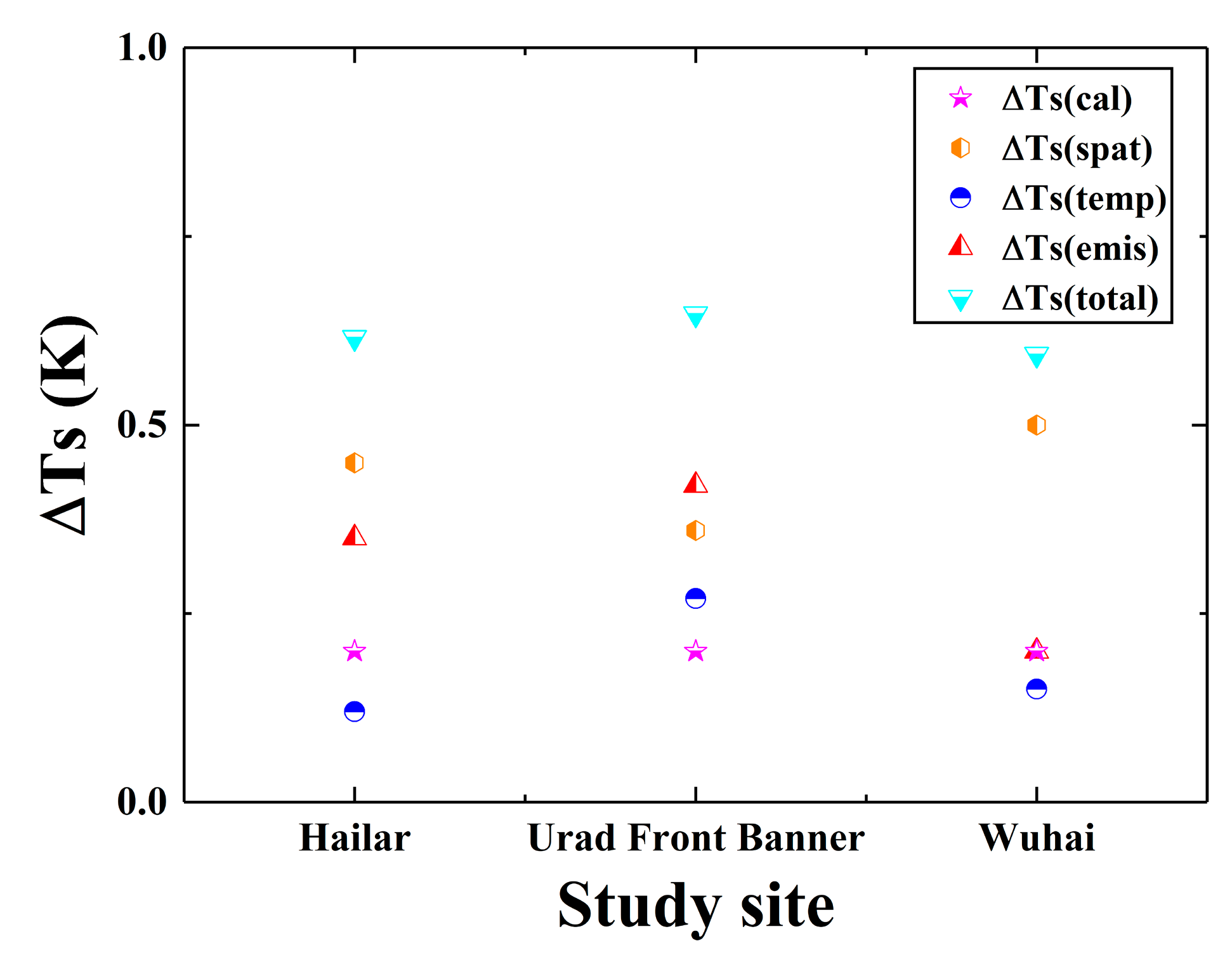
2.1.5. In Situ LST Uncertainty

Prior to the validation of the retrieved LST, it is necessary to know about in situ LST uncertainty. The total in situ LST uncertainty is calculated as the root sum square (RSS) of LST uncertainties that are associated with SI-111 radiometer calibration error, spatial and temporal variability of LST at each site, and surface emissivity measurement error. It is expressed as:
Δ T s ( t o t a l ) = Δ T s ( c a l ) 2 + Δ T s ( s p a t ) 2 + Δ T s ( t e m p ) 2 + Δ T s ( e m i s ) 2
where ΔTs(total) is the total in situ LST uncertainty, ΔTs(cal) is the LST uncertainty that is associated with SI-111 radiometer calibration error, ΔTs(spat) and ΔTs(temp) are the LST uncertainties that are associated with spatial and temporal variability of LST at each site, and ΔTs(emis) is the LST uncertainty that is associated with surface emissivity measurement error.
Each SI-111 radiometer was calibrated by using an NPL blackbody in the laboratory on a one-year cycle. The calibration accuracy was approximately 0.2 K at the temperature range from 263 to 323 K. The spatial variability of LST at each site was evaluated with all available ASTER LST products under clear-sky conditions. The STD of ASTER LST within a 3 × 3 window centered at each site was used to characterize the spatial variability of LST. The STD of in situ LST measurements within 3 min centered at Landsat 8 TIRS acquisition time at each site was used to estimate the temporal variability of LST. The surface emissivity measurement error was assumed to be 0.01, which represents a typical uncertainty in field emissivity measurements over barren surfaces [43].
The in situ LST uncertainties that were caused by different error sources at the Hailar, Urad Front Banner, and Wuhai sites are shown in Figure 3. For each site, the largest error sources were the spatial variability of LST and error in surface emissivity measurement. The total in situ LST uncertainty was less than 0.7 K for all sites.

2.2. Methodology

2.2.1. Single-Channel LST Retrieval Algorithm

The total radiance that was received by a satellite TIR sensor contained three parts: (1) the upwelling radiance of the atmosphere, (2) the surface-emitted radiance attenuated by the atmosphere, and (3) the downwelling atmospheric thermal radiance that was reflected by the surface and attenuated by the atmosphere [44]. The RTE in the TIR region is written as
B i ( T i ) = ε i B i ( T s ) τ i + ( 1 ε i ) L a d , i τ i + L a u , i
where Bi(Ti) is the at-sensor radiance in channel i, Ts is the LST, εi is the surface emissivity in channel i, Lau,i is the atmospheric upwelling radiance in channel i, Lad,i is the atmospheric downwelling radiance in channel i, and τi is the atmospheric transmittance in channel i.
The radiance emitted by the surface can be obtained from the at-sensor radiance by correcting the atmospheric and emissivity effect:
B i ( T s ) = B i ( T i ) ( 1 ε i ) L a d , i τ i L a u , i ε i τ i
The LST can be then retrieved by reversing the Planck function [45].
T s = c 2 λ ln [ c 1 λ 5 B i ( T s ) + 1 ]
where c1 and c2 are radiation constants, and the value and unit of the two constants are 1.191 × 10⁸ W·μm4·sr−1·m-2 and 1.439 × 104 μm·K, respectively.

2.2.2. Calculation of atmospheric parameters

Atmospheric parameters were crucial to retrieve LST from satellite TIR data by using Equations (4) and (5). The reanalysis profiles described in Section 2.1 were provided at different spatial and temporal resolutions. To obtain atmospheric parameters pixel-by-pixel in a satellite TIR image, three main procedures were used to perform the interpolation of the reanalysis profiles in elevation, space, and time, as follows [23,46]. Figure 4 shows the schematic diagram of the interpolation of the reanalysis profiles in space and time.
(1) The reanalysis profile for each grid point at each prescribed UTC time was linearly interpolated in elevation according to surface elevation of each radiosonde station shown in Table 3. The elevation interpolated profile was completed with the MODerate resolution atmospheric TRANsmittance computer code (MODTRAN) built-in midlatitude summer profile up to 100 km.
(2) The reanalysis profiles after elevation interpolation at each prescribed UTC time were further linearly interpolated in space by the geographic latitude and longitude of four grid points closest to each radiosonde station.
(3) The reanalysis profiles after spatial interpolation were further linearly interpolated in time based on two prescribed UTC times closest to Landsat acquisition time.
The UWYO, MYD07, and AIRS, and site-specific interpolated reanalysis profiles were imported into MODTRAN to estimate four atmospheric parameters, i.e., transmittance, upwelling radiance, downwelling radiance, and water vapor content.

2.2.3. Surface Emissivity Estimation

Apart from the atmospheric parameters, surface emissivity is another key parameter with which to retrieve LST from satellite TIR data by using Equations (4) and (5). The emissivity of a pixel can be expressed as the weighted sum of the emissivity of vegetation and bare soil [47,48]:
ε i = P v   ε v i   +   ( 1 P v )   ε s i
where εi is the emissivity of a pixel in channel i, εvi is the emissivity of the vegetation component in channel i, εsi is the emissivity of the soil component in channel i, and Pv is the fractional vegetation coverage whose value can be calculated from the NDVI by using Equation (7) [49]:
P v = [ N D V I N D V I min N D V I max N D V I min ] 2
Where NDVI can be calculated from surface reflectance in the red and NIR channels, and NDVImin and NDVImax represent the NDVI values that corresponded to full soil and vegetation, which were set to 0.05 and 0.85, respectively.
In this research, the surface emissivity in the Landsat 8 TIR channel was estimated in terms of the ASTER GED product. Following the research that was conducted by Hulley et al. [41], the emissivity of the bare soil component can be estimated with the ASTER GED product as follows:
ε s i _ ASTER = ε i _ ASTER P v _ ASTER ε v i _ ASTER ( 1 P v _ ASTER )
where εi_ASTER is the emissivity of the ASTER GED product in channel i and εvi_ASTER is the emissivity of the vegetation component in channel i, whose value can be estimated from the mean emissivity of various types of vegetation in the ASTER spectral library by using the spectral response function of the ASTER channels. Furthermore, εsi_ASTER is the emissivity of the soil component in channel i and Pv_ASTER is the fractional vegetation coverage that can be estimated from the ASTER NDVI by using Equation (7).
To estimate the emissivity of the bare soil component in TIRS channel 10, the emissivity of the TIRS and ASTER channels was fitted to a linear relationship. The coefficients in the linear regression relationship were obtained via multiple regression between soil emissivity in ASTER channels 13 and 14 and TIRS channel 10, which were calculated from several kinds of soil in the ASTER spectral library by using the spectral response function of the ASTER and TIRS channels. The linear regression equation is given as follows:
ε s _ TIRS 10 = 0.443 × ε s _ ASTER 13 + 0.469 × ε s _ ASTER 14 + 0.086
where εs_TIRS10 is the emissivity of the bare soil component in TIRS channel 10, εs_ASTER13 is the emissivity of the bare soil component in ASTER channel 13, and εs_ASTER14 is the emissivity of the bare soil component in ASTER channel 14.
Once the emissivity of the soil component in TIRS channel 10 is available, the emissivity of a pixel in this channel can be calculated as:
ε TIRS 10 = P v _ TIRS ε v _ TIRS 10   +   ( 1 P v _ TIRS )   ε s _ TIRS 10
where εTIRS10 is the emissivity of a pixel in TIRS channel 10, εv_TIRS10 is the emissivity of the vegetation component in TIRS channel 10, which is estimated by averaging the emissivity of various types of vegetation in the ASTER spectral library by using the spectral response function of Landsat 8 TIRS channel 10, and Pv_TIRS is the vegetation coverage that is estimated from NDVI values by using Equation (7). The NDVI value is extracted from reflectance in the red and NIR band from the Landsat 8 surface reflectance product. The flowchart of the estimation of surface emissivity in TIRS channel 10 is shown in Figure 5.

2.2.4. Sensitivity Analysis of Single-Channel Algorithm

The uncertainty of the single-channel algorithm was analyzed in terms of a sensitivity analysis. The total uncertainty in LST that is retrieved by the single-channel algorithm is calculated as the RSS of LST uncertainties that are associated with errors in the atmospheric water vapor and temperature profile, surface emissivity, instrument noise, and RTM. It is expressed as:
Δ T s ( total ) = Δ T s ( W ) 2 + Δ T s ( T a ) 2 + Δ T s ( e m i s ) 2 + Δ T s ( n o i s e ) 2 + Δ T s ( R T M ) 2
where ΔTs(total) is the total uncertainty in LST that is retrieved by the single-channel algorithm; ΔTs(W) and ΔTs(Ta) are the LST uncertainties that are associated with errors in atmospheric water vapor and temperature profile, respectively; ΔTs(emis) is the LST uncertainty that is associated with error in surface emissivity; ΔTs(noise) is the LST uncertainty that is associated with instrument noise; and ΔTs(RTM) is the LST uncertainty that is associated with error in RTM.
Atmospheric effects on the LST that are retrieved by the single-channel algorithm can be simulated in two steps. First, air temperature is increased by 1 K at each atmospheric level. Second, the water vapor mixing ratio is increased by 10% at each atmospheric level. These variations represent typical uncertainties in the atmospheric profile [31]. The surface emissivity error is assumed to be 0.01, which is a typical uncertainty in surface emissivity estimation [50]. LST uncertainty that is associated with the RTM error of MODTRAN can be assumed to be 0.2 K. The instrument noise (NEΔT) is approximately 0.05 K in Landsat 8 TIRS band 10 [14].
To evaluate the uncertainty of the single-channel algorithm under different water vapor content (WVC) conditions, six MODTRAN standard atmospheres were used in the sensitivity analysis. The results are shown in Figure 6. For each atmosphere, the largest error source is the uncertainty in atmospheric water vapor and temperature profile, whereas the surface emissivity error has a relatively small influence on the LST that is retrieved by the single-channel algorithm. The total LST error is less than 1 K for an atmospheric WVC smaller than 3 g/cm2. However, it dramatically increases to 2 K for a tropical atmosphere with an atmospheric WVC of approximately 4 g/cm2.

3. Results

3.1. Comparison of Vertical Distributions of Different Atmospheric Profiles

To analyze the performances of different atmospheric profiles, the vertical distribution of air temperature and dew point temperature that was extracted from the atmospheric profiles of 1 January 2018 at Bucuresti lnmh-Banesa station, 30 April 2018 at Istanbul station, and 11 August 2018 at Izmir station is displayed in Figure 7. These profiles on the three dates were used to represent different atmospheric situations with WVCs of 1.5, 2.5, and 3.4 g/cm2.
Except for the MYD07 profile, there were small discrepancies between the vertical distribution of air temperature extracted from the UWYO profile and the other atmospheric profiles below 50 km (approximately 1–1000 hPa). The differences between the air temperatures that were extracted from the UWYO and MYD07 profiles below 5 km (approximately 500–1000 hPa) ranged from 3 to 7 K. A relatively large discrepancy of 2–5 K between 10 and 30 km (approximately 10–300 hPa) could also be observed.
Compared with air temperature, the discrepancies of the vertical distribution of dew point temperatures that were extracted from different atmospheric profiles were larger. Except for the AIRS profile, the differences between the dew point temperatures that were extracted from the UWYO profile and the other profiles from 10 to 50 km (approximately 1–300 hPa) were as much as 12 K. The largest difference for the AIRS profile was higher than 40 K. There were relatively large discrepancies of 5–8 K between the dew point temperatures that were extracted from the UWYO profile and the other profiles from 2 to 5 km (approximately 500–800 hPa).

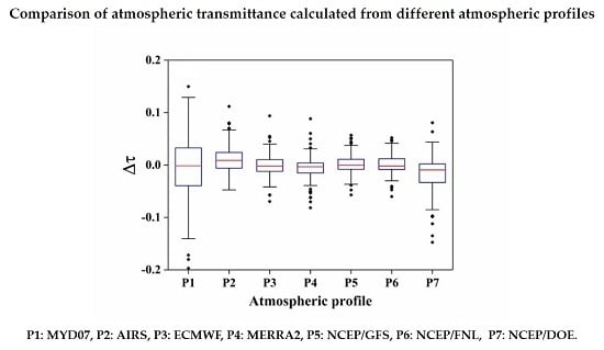
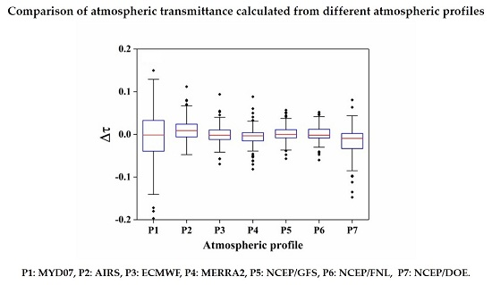
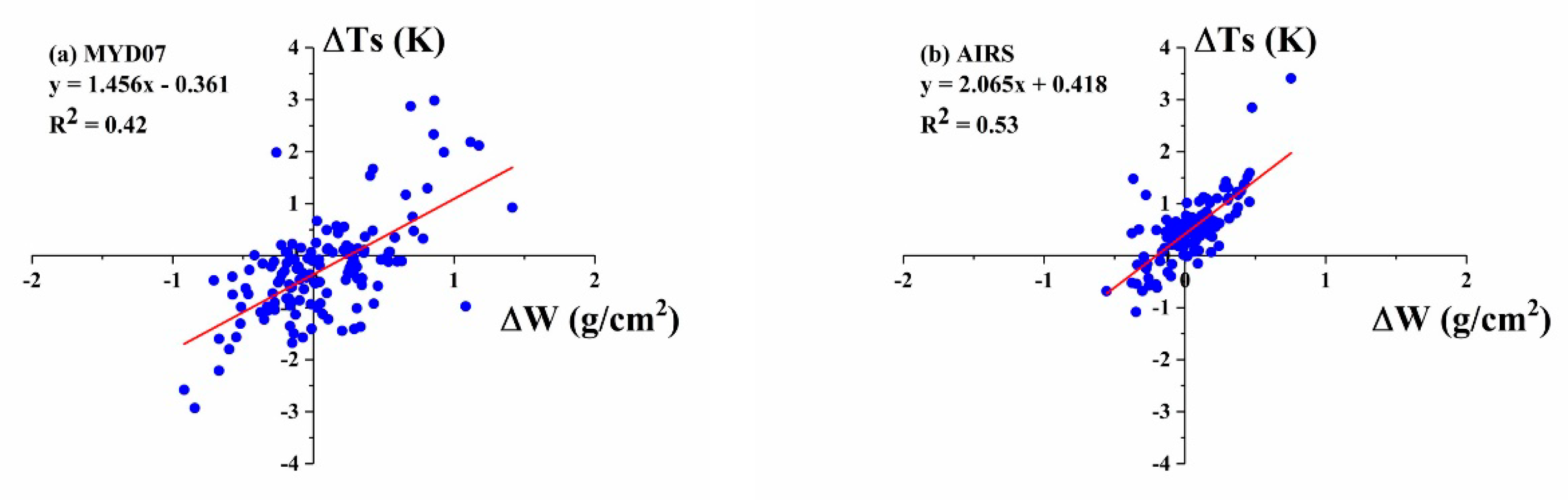
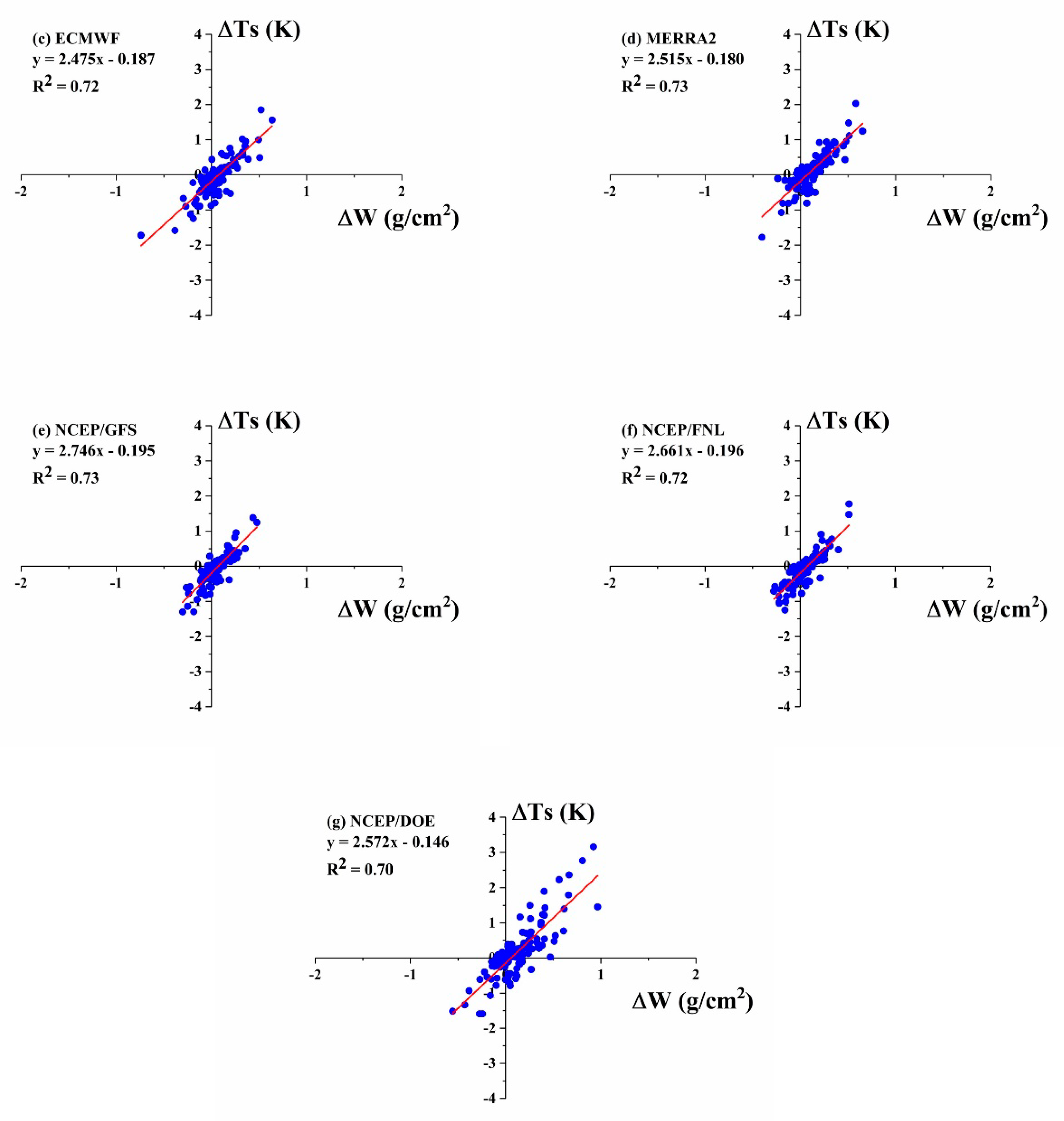
3.2. Comparison of Atmospheric Parameters Calculated from Different Atmospheric Profiles

The UWYO radio sounding profile was used as reference data to evaluate the accuracies of the other seven atmospheric profiles at the 17 radiosonde stations shown in Table 3. All atmospheric profiles were input into MODTRAN 5.2 to calculate four atmospheric parameters: atmospheric transmittance, upwelling radiance, downwelling radiance, and WVC.
Figure 8 shows the boxplots of the differences between atmospheric parameters that were calculated from the UWYO profile and the other seven atmospheric profiles. The corresponding root-mean-square error (RMSE) values of the differences between atmospheric parameters that were calculated from the UWYO profile and the other seven atmospheric profiles are summarized in Table 4.
Compared with the UWYO profile, the worst accuracy of the estimated atmospheric parameters was obtained for the MYD07 profile, with RMSE values of approximately 0.06, 0.5 W/m2/sr/μm, 0.7 W/m2/sr/μm, and 0.4 g/cm2 for atmospheric transmittance, upwelling radiance, downwelling radiance, and WVC, respectively. The RMSE values of these parameters were higher than all reanalysis profiles. Even if the NCEP/DOE profile had the lowest spatial and vertical resolution, the accuracy of atmospheric parameters was the lowest of all reanalysis profiles. It is worth noting that its accuracy was still higher than the MYD07 profile. Though the spatial resolution of the MYD07 profile was the highest in all satellite-derived or reanalysis profiles, only 11 infrared bands (bands 25 and 27–36) were used for the retrieval of the MYD07 profile [51], which led to a low accuracy of air temperature and dew point temperature. There are 2378 spectral bands between 3.7 and 15 μm to retrieve the AIRS profile [35,52]. Therefore, the accuracy of atmospheric parameters that were estimated from the AIRS profile was better than that of atmospheric parameters that were obtained from the MYD07 profile.

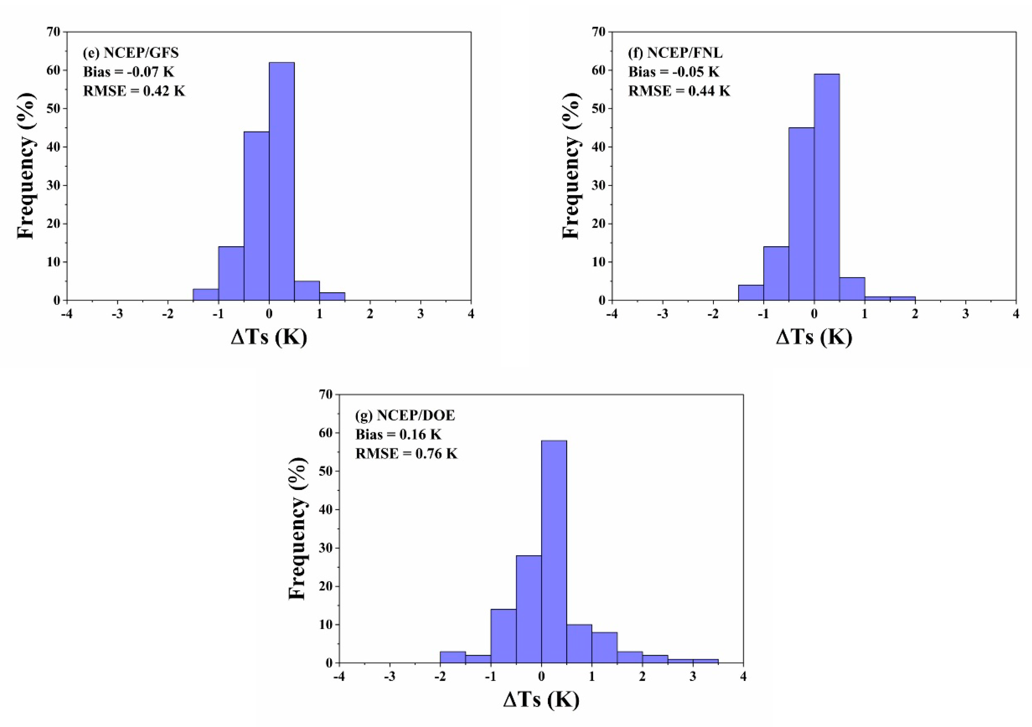
3.3. Comparison of Retrieved LST Using Different Atmospheric Profiles

To further evaluate the accuracy of the atmospheric profiles, the retrieved LST that used the UWYO profile was used as reference data to compare those using the other seven atmospheric profiles. Except for the atmospheric parameters that were calculated from different atmospheric profiles, the other parameters in Equations (4) and (5) were the same for all atmospheric profiles. Thus, the differences between the retrieved LST that used the UWYO profile and the other seven atmospheric profiles were caused by the discrepancies between the UWYO profile and the other seven atmospheric profiles.
The histograms of the differences between the retrieved LST that used the UWYO profile and the other seven atmospheric profiles are shown in Figure 9. For all profiles, the LST differences were located in the range between -1 and 1 K in most cases. Relatively large LST differences could also be observed for the MYD07, AIRS, and NCEP/DOE profiles. The RMSE values were smaller than 0.6 K for the ECMWF, MERRA2, NCEP/GFS, and NCEP/FNL profiles. The worst accuracy was obtained with the MYD07 profile with an RMSE value of 1 K.
The relationships between LST differences (ΔTs = Ts_other - Ts_UWYO) and atmospheric WVC differences (ΔW = Wother - WUWYO) were further examined for all atmospheric profiles. Figure 10 displays the scatterplots of LST differences versus atmospheric WVC differences between the UWYO profile and the other seven atmospheric profiles. The coefficient of determination (R2) was higher than 0.7 for all the reanalysis profiles. The results indicated that more than 70% of the variation in ΔTs could be explained by ΔW for all of the reanalysis profiles. Relatively low values of R2 were obtained for the MYD07 and AIRS profiles. The results showed that only approximately 50% of the variation in ΔTs was explained by ΔW.

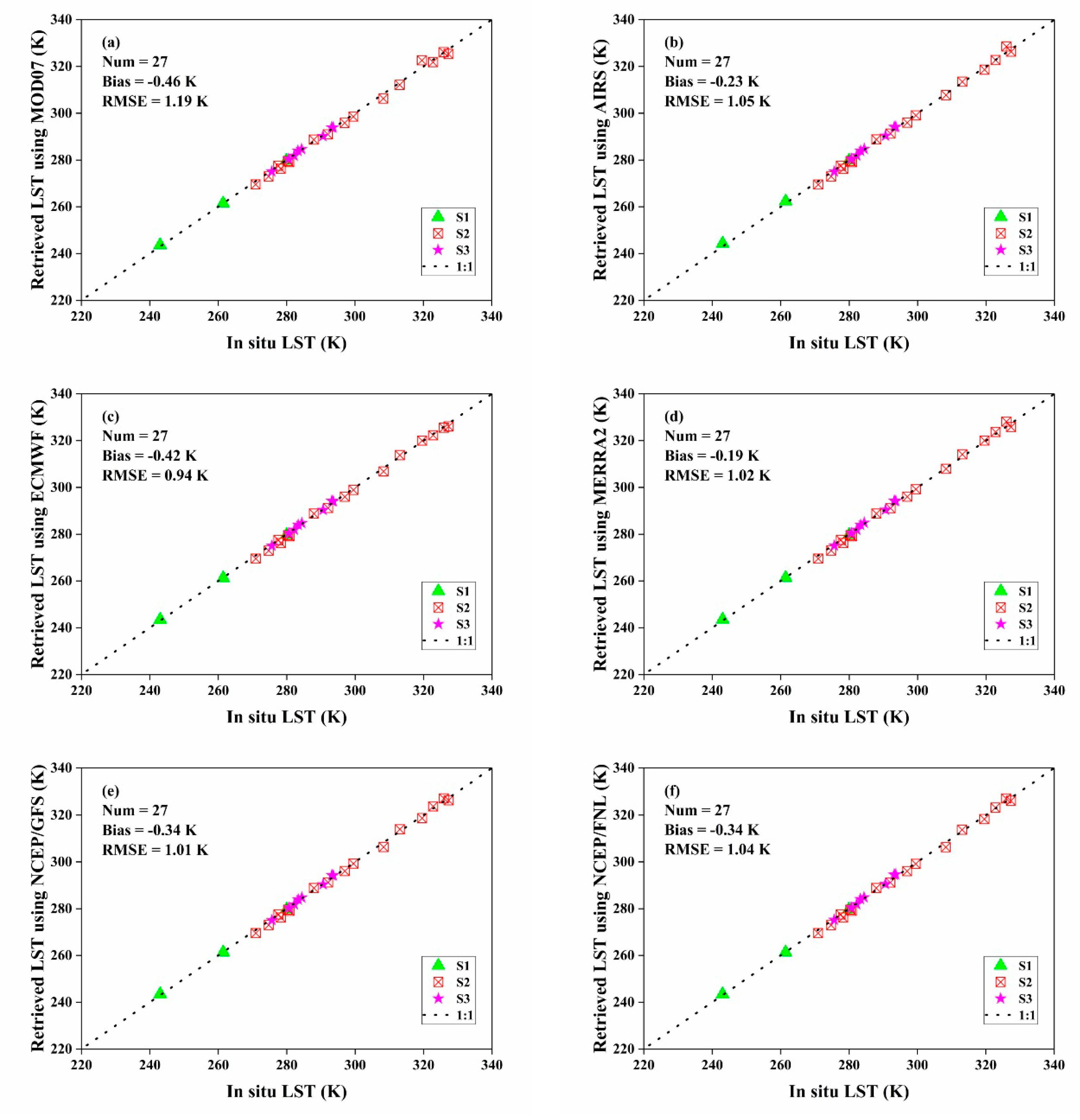
3.4. LST Validation Using in Situ Measurements

In situ LST measurements that were collected at the Hailar, Urad Front Banner, and Wuhai sites were used to validate the retrieved LST that used different atmospheric profiles. There are no radiosonde stations available at the three sites. Therefore, the UWYO profile was not used. Furthermore, there was a smaller temporal gap between the overpassing time of Terra/MODIS and Landsat 8/TIRS at the three sites. Therefore, the MOD07 profile, rather than the MYD07 profile, was used.
The scatterplots of the retrieved LST that used different atmospheric profiles versus the in situ LST at the three sites are shown in Figure 11. Compared with the in situ LST, the accuracy of the retrieved LST that used different atmospheric profiles was approximately 1.0–1.5 K. The worst accuracy of the retrieved LST was obtained for the NCEP/DOE profile, with a bias and RMSE of approximately −0.7 and 1.5 K, respectively. These results can be attributed to the lower spatial resolution of 2.5° × 2.5° and vertical resolution of 17 levels for the NCEP/DOE profile. Similar RMSE values of approximately 1.0 K were achieved for the ECMWF, MERRA2, NCEP/GFS, and NCEP/FNL profiles.
The bias and RMSE of the differences between the retrieved LST that used different atmospheric profiles and the in situ LST at the three sites are summarized in Table 5. The mean atmospheric WVC for each site is also listed in Table 5. The RMSE values for all atmospheric profiles at the Urad Front Banner site were larger than those at the Hailar and Wuhai sites. Two possible reasons could explain this result. First, the uncertainty of the in situ LST in the Urad Front Banner site was relatively large, which we can see from Figure 3. Second, the atmospheric WVC of the Urad Front Banner site was relatively large, reaching 0.90 g / cm2. As shown in Figure 6, a larger total uncertainty in LST that was retrieved by the single-channel algorithm was obtained at a larger atmospheric WVC. Compared with the in situ LST, the accuracies of the retrieved LST that used the ECMWF, MERRA2, NCEP/GFS, and NCEP/FNL profiles were better than those that used the MOD07, AIRS, and NCEP/DOE profiles.

4. Discussion

In general, the vertical distributions of air temperature and dew point temperature that were extracted from the reanalysis profiles were more similar than those from the satellite-derived profiles (i.e., MYD07 and AIRS) when using the UWYO profile as reference data. As shown in Figure 7, the difference between the satellite-derived profiles and the UWYO profile was approximately twice the difference between the reanalysis profiles and UWYO profile, regardless of the vertical distribution of air temperature or dew point temperature. The reason for this may be because the reanalysis profiles, which were the results of four-dimensional assimilation of meteorological data, including radiosonde, ground, and satellite measurements, were more representative of the real atmospheric situation than the satellite-derived profiles from satellite measurements from a single source.
The accuracy of the atmospheric parameters that were estimated from the four reanalysis profiles (i.e., ECMWF, MERRA2, NCEP/GFS, and NCEP/FNL) was better than that of the atmospheric parameters that were obtained from the two satellite-derived profiles (i.e., MYD07 and AIRS). As shown in Figure 8 and Table 4, the RMSE values of the atmospheric parameters of these four reanalysis profiles were less than 0.025, 0.2 W/m2/sr/μm, 0.3 W/m2/sr/μm, and 0.2 g/cm2 for atmospheric transmittance, upwelling radiance, downwelling radiance, and WVC, respectively. The result could be explained by the reason that the satellite-derived profiles that were temporally and spatially closest to each radiosonde station were used in this study, whereas temporal and spatial interpolation was performed for the reanalysis profiles, which may better represent real atmospheric conditions at the radiosonde stations.
When using the LST that was calculated by UWYO atmospheric profile as reference data to compare the other seven atmospheric profiles, the accuracy of reanalysis profiles were relatively good, and MYD07 had the worst accuracy. The reason for this may be that the atmospheric parameters (transmittance, upwelling radiance, and downwelling radiance) in the TIR region were dependent not only on the total amount of atmospheric WVC but also on the vertical distribution of water vapor and temperature profile. As shown in Figure 7 and Table 4, the discrepancy of the vertical distribution between the MYD07 profile and the UWYO profile was the largest. Furthermore, compared with the UWYO profile, the RMSE value of the atmospheric parameters that were calculated by the MYD07 profile was the largest.
Despite the findings of this study, there are still some limitations. (1) Only five types of reanalysis atmospheric profile data were selected in this study, and more reanalysis atmospheric profiles such as the Japanese 55-year Reanalysis Data (JRA-55) were not included in the scope of the study. In addition, this article used ERA-Interim data, but now with the time resolution of the new ERA5 data is higher, which may improve the accuracy of the atmospheric profile. (2) The uncertainty analysis of the UWYO profile was not analyzed, and it was directly used as comparative data. (3) LST validation was only performed at three sites with limited land cover types, and the results may not have been widely representative.

5. Conclusions

In this study, the performances of seven atmospheric profiles from different sources (MYD07, AIRS, ECMWF, MERRA2, NCEP/GFS, NCEP/FNL, and NCEP/DOE) were evaluated in the single-channel algorithm for LST retrieval from Landsat 8 TIRS data. The UWYO profile that was collected at 17 radiosonde stations was used as reference data to evaluate the accuracies of the seven atmospheric profiles. Furthermore, in situ LST measurements that were collected at the Hailar, Urad Front Banner, and Wuhai sites were further used to validate the accuracies of the retrieved LST that used the seven atmospheric profiles. Some conclusions were drawn, as follows.
(1) The vertical distributions of air temperature and dew point temperature profiles extracted from the reanalysis profiles (i.e., ECMWF, MERRA2, NCEP/GFS, and NCEP/FNL) were more similar than those from the satellite-derived profiles (i.e., MYD07 and AIRS) when using the UWYO profile as reference data. The largest discrepancy of the vertical distribution of air temperature and dew point temperature profiles was observed between the MYD07 and UWYO profiles.
(2) Compared with the UWYO profile, the accuracies of atmospheric parameters for the ECMWF, MERRA2, NCEP/GFS, and NCEP/FNL profiles were better than those for the MYD07, AIRS, and NCEP/DOE profiles. The worst accuracy of atmospheric parameters was obtained for the MYD07 profile, with RMSE values of approximately 0.06, 0.5 W/m2/sr/μm, 0.7 W/m2/sr/μm, and 0.4 g/cm2 for atmospheric transmittance, upwelling radiance, downwelling radiance, and WVC, respectively.
(3) Compared with the UWYO profile, the RMSE values (approximately 0.5 K) of the retrieved LST that used the ECMWF, MERRA2, NCEP/GFS, and NCEP/FNL profiles were smaller than those (larger than 0.8 K) that used the MYD07, AIRS, and NCEP/DOE profiles. The worst accuracy of the retrieved LST was obtained for the MYD07 profile, with an RMSE value of approximately 1.0 K.
(4) Compared with the in situ LST, the RMSE values of the retrieved LST that used the ECMWF, MERRA2, NCEP/GFS, and NCEP/FNL profiles were approximately 1.0 K. The worse accuracy of the retrieved LST was obtained for the NCEP/DOE profile, with an RMSE value of approximately 1.5 K.
In general, the performances of the ECMWF, MERRA2, NCEP/GFS, and NCEP/FNL profiles were better than those of the MYD07, AIRS, and NCEP/DOE profiles. Therefore, the ECMWF, MERRA2, NCEP/GFS, and NCEP/FNL profiles had great potential to perform accurate atmospheric correction for the generation of long-term time series LST products from Landsat TIR data by using the single-channel algorithm.

Author Contributions

Conceptualization, S.-B.D.; Methodology, S.-B.D., and J.Y.; Software, J.Y.; Validation, J.Y., S.-B.D.; Formal analysis, J.Y.; Investigation, J.Y.; Resources, X.Z., M.G., P.L., and P.W.; Data curation, J.Y. and S.-B.D.; Writing—original draft preparation, J.Y.; Writing—review and editing, S.-B.D. and C.H.; Supervision, S.-B.D.; Funding acquisition, S.-B.D. All authors have read and agreed to the published version of the manuscript.

Funding

This research was funded by the National Key R&D Program of China, 2018YFB0504800 (2018YFB0504804), by the National Natural Science Foundation of China, grant numbers 41871275 and 41921001.

Acknowledgments

The radio sounding profile used in this study was downloaded from the University of Wyoming website (http://weather.uwyo.edu/upperair/sounding.html). MxD07 profile data, AIRS profile data and ASTER GED product were downloaded from NASA’s Earth Observing System Data and Information System (EOSDIS) website (https://search.earthdata.nasa.gov/search). ECMWF profile was downloaded from the European Centre for Medium-Range Weather Forecasts website (http://apps.ecmwf.int/datasets/). MERRA2 profile was downloaded from the Goddard Earth Observing System Model (GEOS-5) combined with its Atmospheric Data Assimilation System (ADAS) website (https://disc.gsfc.nasa.gov). NCEP/GFS profile was downloaded from the National Centers for Environmental Prediction (NCEP) website (https://nomads.ncdc.noaa.gov/data/gfsanl/). NCEP/FNL profile was downloaded from the global data assimilation system (GDAS) website (http://rda.ucar.edu/datasets/ds083.2/). NCEP/DOE profile was downloaded from the NCEP/DOE Reanalysis 2 (R2) Project website (http://rda.ucar.edu/datasets/ds091.0/). The at-sensor radiance data, TIR data and Landsat 8 OLI surface reflectance product were downloaded from the NASA Earth data website (https://earthexplorer.usgs.gov).

Conflicts of Interest

The authors declare no conflict of interest.

References

  1. Anderson, M.C.; Norman, J.M.; Diak, G.R.; Kustas, W.P.; Mecikalski, J.R. A two-source time-integrated model for estimating surface fluxes using thermal infrared remote sensing. Remote Sens. Environ. 1997, 60, 195–216. [Google Scholar] [CrossRef]
  2. Anderson, M.C.; Kustas, W.P.; Norman, J.M.; Hain, C.R.; Mecikalski, J.R.; Schultz, L.; González-Dugo, M.P.; Cammalleri, C.; d’Urso, G.; Pimstein, A.; et al. Mapping daily evapotranspiration at field to continental scales using geostationary and polar orbiting satellite imagery. Hydrol. Earth Syst. Sci. 2011, 15, 223–239. [Google Scholar] [CrossRef] [Green Version]
  3. Zhou, L.; Dickinson, R.E.; Tian, Y.; Jin, M.; Ogawa, K.; Yu, H.; Schmugge, T. A sensitivity study of climate and energy balance simulations with use of satellite-derived emissivity data over Northern Africa and the Arabian Peninsula. J. Geophys. Res Atmos. 2003, 108, 4795–4803. [Google Scholar] [CrossRef] [Green Version]
  4. Duan, S.-B.; Li, Z.-L.; Wang, C.; Zhang, S.; Tang, B.-H.; Leng, P.; Gao, M.-F. Land-surface temperature retrieval from Landsat 8 single-channel thermal infrared data in combination with NCEP reanalysis data and ASTER GED product. Int. J. Remote Sens. 2019, 40, 1763–1778. [Google Scholar] [CrossRef]
  5. Wan, Z.; Wang, P.; Li, X. Using MODIS land surface temperature and normalized difference vegetation index products for monitoring drought in the southern Great Plains, USA. Int. J. Remote Sens. 2004, 25, 61–72. [Google Scholar] [CrossRef]
  6. Weng, Q. Thermal infrared remote sensing for urban climate and environmental studies: Methods, applications, and trends. ISPRS J. Photogramm. 2009, 64, 335–344. [Google Scholar] [CrossRef]
  7. Anderson, M.C.; Norman, J.M.; Kustas, W.P.; Houborg, R.; Starks, P.J.; Agam, N. A thermal-based remote sensing technique for routine mapping of land-surface carbon, water and energy fluxes from field to regional scales. Remote Sens. Environ. 2008, 112, 4227–4241. [Google Scholar] [CrossRef]
  8. Prata, A.J.; Caselles, V.; Coll, C.; Sobrino, J.A.; OttlO, C. Thermal remote sensing of land surface temperature from satellites: Current status and future prospects. Remote Sens Reviews. 1995, 12, 175–224. [Google Scholar] [CrossRef]
  9. Dash, P.; Göttsche, F.-M.; Olesen, F.-S.; Fischer, H. Land surface temperature and emissivity estimation from passive sensor data: Theory and practice-current trends. Int. J. Remote Sens. 2002, 23, 2563–2594. [Google Scholar] [CrossRef]
  10. Duan, S.-B.; Li, Z.-L.; Tang, B.-H.; Wu, H.; Tang, R. Generation of a time-consistent land surface temperature product from MODIS data. Remote Sens. Environ. 2014, 140, 339–349. [Google Scholar] [CrossRef]
  11. Duan, S.-B.; Li, Z.-L.; Leng, P. A framework for the retrieval of all-weather land surface temperature at a high spatial resolution from polar-orbiting thermal infrared and passive microwave data. Remote Sens. Environ. 2017, 195, 107–117. [Google Scholar] [CrossRef]
  12. Malakar, N.K.; Hulley, G.C.; Hook, S.J.; Laraby, K.; Cook, M.; Schott, J.R. An operational land surface temperature product for Landsat thermal data: Methodology and validation. IEEE Trans. Geosci. Remote Sens. 2018, 56, 5717–5735. [Google Scholar] [CrossRef]
  13. Barsi, J.A.; Schott, J.R.; Hook, S.J.; Raqueno, N.G.; Markham, B.L.; Radocinski, R.G. Landsat-8 thermal infrared sensor (TIRS) vicarious radiometric calibration. Remote Sens. 2014, 6, 11607–11626. [Google Scholar] [CrossRef] [Green Version]
  14. Montanaro, M.; Levy, R.; Markham, B. On-orbit radiometric performance of the Landsat 8 thermal infrared sensor. Remote Sens. 2014, 6, 11753–11769. [Google Scholar] [CrossRef] [Green Version]
  15. Isaya Ndossi, M.; Avdan, U. Application of open source coding technologies in the production of land surface temperature (LST) maps from Landsat: A PyQGIS plugin. Remote Sens. 2016, 8, 413. [Google Scholar] [CrossRef] [Green Version]
  16. Wang, M.; Zhang, Z.; He, G.; Wang, G.; Long, T.; Peng, Y. An enhanced single-channel algorithm for retrieving land surface temperature from Landsat series data. J. Geophys. Res Atmos. 2016, 121, 11712–11722. [Google Scholar] [CrossRef]
  17. Duan, S.-B.; Li, Z.-L.; Li, H.; Göttsche, F.-M.; Wu, H.; Zhao, W.; Leng, P.; Zhang, X.; Coll, C. Validation of Collection 6 MODIS land surface temperature product using in situ measurements. Remote Sens. Environ. 2019, 225, 16–29. [Google Scholar] [CrossRef] [Green Version]
  18. Qin, Z.; Karnieli, A.; Berliner, P. A mono-window algorithm for retrieving land surface temperature from Landsat TM data and its application to the Israel-Egypt border region. Int. J. Remote Sens. 2010, 22, 3719–3746. [Google Scholar] [CrossRef]
  19. Wang, F.; Qin, Z.; Song, C.; Tu, L.; Karnieli, A.; Zhao, S. An improved mono-window algorithm for land surface temperature retrieval from landsat 8 thermal infrared sensor data. Remote Sens. 2015, 7, 4268–4289. [Google Scholar] [CrossRef] [Green Version]
  20. Jiménez-Muñoz, J.C.; Sobrino, J.A. A generalized single-channel method for retrieving l surface temperature from remote sensing data. J. Geophys. Res Atmos. 2003, 109, 4688. [Google Scholar] [CrossRef] [Green Version]
  21. Jiménez-Muñoz, J.C.; Cristóbal, J.; Sobrino, J.A.; Sòria, G.; Ninyerola, M.; Pons, X. Revision of the single-channel algorithm for land surface temperature retrieval from Landsat thermal-infrared data. IEEE Trans. Geosci. Remote Sens. 2009, 47, 339–349. [Google Scholar] [CrossRef]
  22. Cristdoi, J.; Jiménez-Muñoz, J.C.; Sobrino, J.A.; Ninyerola, M.; Pons, X. Improvements in land surface temperature retrieval from the Landsat series thermal band using water vapor and air temperature. J. Geophys. Res Atmos. 2009, 114, D08103. [Google Scholar] [CrossRef]
  23. Barsi, J.A.; Barker, J.L.; Schott, J.R. An atmospheric correction parameter calculator for a single thermal band rarth-sensing instrument. IGARSS 2003 2003, 5, 3014–3016. [Google Scholar] [CrossRef]
  24. Sobrino, J.A.; Jiménez-Muñoz, J.C.; Paolini, L. Land surface temperature retrieval from LANDSAT TM 5. Remote Sens. Environ. 2004, 90, 434–440. [Google Scholar] [CrossRef]
  25. Yu, X.; Guo, X.; Wu, Z. Land surface temperature retrieval from Landsat 8 TIRS-Comparison between radiative transfer equation-based method, split window algorithm and single channel method. Remote Sens. 2014, 6, 9829–9852. [Google Scholar] [CrossRef] [Green Version]
  26. Windahl, E.; de Beurs, K. An intercomparison of Landsat land surface temperature retrieval methods under variable atmospheric conditions using in situ skin temperature. Int. J. Appl. Earth Obs. 2016, 51, 11–27. [Google Scholar] [CrossRef] [Green Version]
  27. Wang, A.; Zeng, X. Evaluation of multireanalysis products with in situ observations over the Tibetan Plateau. J. Geophys. Res Atmos. 2012, 117, D05102. [Google Scholar] [CrossRef]
  28. Jiménez-Muñoz, J.C.; Sobrino, J.A.; Mattar, C.; Franch, B. Atmospheric correction of optical imagery from MODIS and reanalysis atmospheric products. Remote Sens. Environ. 2010, 114, 2195–2210. [Google Scholar] [CrossRef]
  29. Sobrino, J.A.; Jiménez-Muñoz, J.C.; Mattar, C.; Sòria, G. Evaluation of Terra/MODIS atmospheric profiles product (MOD07) over the Iberian Peninsula: A comparison with radiosonde stations. Int. J. Digit. Earth. 2014, 8, 771–783. [Google Scholar] [CrossRef]
  30. Meng, X.; Cheng, J. Evaluating eight global reanalysis products for atmospheric correction of thermal infrared sensor-Application to Landsat 8 TIRS10 data. Remote Sens. 2018, 10, 474. [Google Scholar] [CrossRef] [Green Version]
  31. Coll, C.; Caselles, V.; Valor, E.; Nicl, R. Comparison between different sources of atmospheric profiles for land surface temperature retrieval from single channel thermal infrared data. Remote Sens. Environ. 2012, 117, 199–210. [Google Scholar] [CrossRef]
  32. Li, H.; Liu, Q.; Du, Y.; Jiang, J.; Wang, H. Evaluation of the NCEP and MODIS atmospheric products for single channel land surface temperature retrieval with ground measurements: A case study of HJ-1B IRS data. IEEE J. STARS. 2013, 6, 1399–1408. [Google Scholar] [CrossRef]
  33. PjstarPlanells, L.; Garc-Santos, V.; Caselles, V. Comparing different profiles to characterize the atmosphere for three MODIS TIR bands. Atmos. Res. 2015, 161, 108–115. [Google Scholar] [CrossRef] [Green Version]
  34. Crosson, W.L.; Al-Hamdan, M.Z.; Hemmings, S.N.J.; Wade, G.M. A daily merged MODIS Aqua-Terra land surface temperature data set for the conterminous United States. Remote Sens. Environ. 2012, 119, 315–324. [Google Scholar] [CrossRef]
  35. Aumann, H.H.; Chahine, M.T.; Gautier, C.; Goldberg, M.D.; Kalnay, E.; McMillin, L.M.; Revercomb, H.; Rosenkranz, P.W.; Smith, W.L.; Staelin, D.H.; et al. AIRS/AMSU/HSB on the Aqua mission: Design, science objective, data products, and processing systems. IEEE Trans. Geosci. Remote Sens. 2003, 41, 253–264. [Google Scholar] [CrossRef] [Green Version]
  36. Fotsing Talla, C.; Njomo, D.; Cornet, C.; Dubuisson, P.; Akana Nguimdo, L. ECMWF atmospheric profiles in Maroua, Cameroon: Analysis and overview of the simulation of downward global solar radiation. Atmosphere 2018, 9, 44. [Google Scholar] [CrossRef] [Green Version]
  37. Molod, A.; Takacs, L.; Suarez, M.; Bacmeister, J. Development of the GEOS-5 atmospheric general circulation model: Evolution from MERRA to MERRA2. Geosci. Model Dev. 2015, 8, 1339–1356. [Google Scholar] [CrossRef] [Green Version]
  38. Zia ul Rehman, T.; Muhammad, A.; Muhammad, A.; Nasir, H.; Hamza, S.; Hasnain, A. Evaluation of NCEP-Products (NCEP-NCAR, NCEP-DOE, NCEP-FNL, NCEP-GFS) of solar radiation for Karachi, Pakistan. ISES 2018, 1–12. [Google Scholar] [CrossRef]
  39. Eom, H.-S.; Myoung-Seok, S. Seasonal and diurnal variations of stability indices and environmental parameters using NCEP FNL data over East Asia. Asia Pac. J. Atmos. Sci. 2011, 47, 181–192. [Google Scholar] [CrossRef]
  40. Lim, Y.-K.; Stefanova, L.B.; Chan, S.C.; Schubert, S.D.; Ochubert, S.J. High-resolution subtropical summer precipitation derived from dynamical downscaling of the NCEP/DOE reanalysis: How much small-scale information is added by a regional model? Clim. Dynam. 2010, 37, 1061–1080. [Google Scholar] [CrossRef]
  41. Hulley, G.C.; Hook, S.J.; Abbott, E.; Malakar, N.; Islam, T.; Abrams, M. The ASTER Global Emissivity Dataset (ASTER GED): Mapping Earth’s emissivity at 100 meter spatial scale. Geophys. Res. Lett. 2015, 42, 7966–7976. [Google Scholar] [CrossRef]
  42. Wang, C.; Duan, S.-B.; Zhang, X.; Wu, H.; Gao, M.-F.; Leng, P. An alternative split-window algorithm for retrieving land surface temperature from Visible Infrared Imaging Radiometer Suite data. Int. J. Remote Sens. 2019, 40, 1640–1654. [Google Scholar] [CrossRef]
  43. Rubio, E.; Caselles, V.; Coll, C.; Valour, E.; Sospedra, F. Thermal-infrared emissivities of natural surfaces: Improvements on the experimental set-up and new measurements. Int. J. Remote Sens. 2003, 24, 5379–5390. [Google Scholar] [CrossRef]
  44. Li, Z.-L.; Tang, B.-H.; Wu, H.; Ren, H.; Yan, G.; Wan, Z.; Trigo, I.F.; Sobrino, J.A. Satellite-derived land surface temperature: Current status and perspectives. Remote Sens. Environ. 2013, 131, 14–37. [Google Scholar] [CrossRef] [Green Version]
  45. Li, F.; Jackson, T.J.; Kustas, W.P.; Schmugge, T.J.; French, A.N.; Cosh, M.H.; Bindlish, R. Deriving land surface temperature from landsat 5 and 7 during SMEX02/SMACEX. Remote Sens. Environ. 2004, 92, 521–534. [Google Scholar] [CrossRef]
  46. Rosas, J.; Houborg, R.; McCabe, M.F. Sensitivity of Landsat 8 Surface Temperature Estimates to Atmospheric Profile Data: A Study Using MODTRAN in Dryland Irrigated Systems. Remote Sens. 2017, 9, 988. [Google Scholar] [CrossRef] [Green Version]
  47. Sobrino, J.A.; Caselles, V.; Becker, F. Significance of the remotely sensed thermal infrared measurements obtained over a citrus orchard. ISPRS J. Photogramm. 1990, 44, 343–354. [Google Scholar] [CrossRef]
  48. Valor, E.; Caselles, V. Mapping land surface emissivity from NDVI: Application to European, African, and South American areas. Remote Sens. Environ. 1996, 57, 167–184. [Google Scholar] [CrossRef]
  49. Carlson, T.N.; Perry, E.M.; Schmugge, T.J. Remote estimation of soil moisture availability and fractional vegetation cover for agricultural fields. Agr. Forest Meteorol. 1990, 52, 45–69. [Google Scholar] [CrossRef]
  50. Li, Z.-L.; Wu, H.; Wang, N.; Qiu, S.; Sobrino, J.A.; Wan, Z.; Tang, B.-H.; Yan, G. Land surface emissivity retrieval from satellite data. Int. J. Remote Sens. 2013, 34, 3084–3127. [Google Scholar] [CrossRef]
  51. Seemann, S.W.; Borbas, E.E.; Li, J.; Menzel, W.P.; Gumley, L.E. MODIS atmospheric profile retrieval algorithm theoretical basis document; Cooperative Institute for Meteorological Satellite Studies: University of Wisconsin-Madison, Madison, WI, USA, 2006. [Google Scholar]
  52. Susskind, J.; Barnet, C.D.; Blaisdell, J.M. Retrieval of atmospheric and surface parameters from AIRS/AMSU/HSB under cloudy conditions. IEEE Trans. Geosci. Remote Sens. 2003, 41, 390–409. [Google Scholar] [CrossRef]
Figure 1. Geographical location of 17 radiosonde stations.
Remotesensing 12 00791 g001
Figure 2. Geolocation of three study sites for land surface temperature (LST) validation.
Remotesensing 12 00791 g002
Figure 3. In situ LST uncertainties that were caused by different error sources at Hailar, Urad Front Banner, and Wuhai sites.
Remotesensing 12 00791 g003
Figure 4. Schematic diagram of the interpolation of the reanalysis profiles in space and time (adapted from Barsi et al. [23]): (x, y), (x, y + 1), (x + 1, y + 1), and (x + 1, y) are the coordinates of the four grid corners surrounding a site. A pentagram or circle in red represents the coordinate of a site, t0 is the satellite overpassing time, and t1 and t2 are the prescribed UTC time of the reanalysis profiles before and after satellite overpassing time.
Remotesensing 12 00791 g004
Figure 5. Flowchart of the estimation of surface emissivity in TIRS channel 10.
Remotesensing 12 00791 g005
Figure 6. Uncertainties in LST retrieved by the single-channel algorithm due to different error sources under six MODTRAN standard atmosphere conditions—SAW: subarctic winter atmosphere, MLW: midlatitude winter atmosphere, USS: 1976 US standard atmosphere, SAS: subarctic summer atmosphere, MLS: midlatitude summer atmosphere, and TRO: tropical atmosphere.
Remotesensing 12 00791 g006
Figure 7. Comparison of vertical distribution of air temperature—(a), (c), and (e)—and dew point temperature—(b), (d), and (f)—values that were extracted from different atmospheric profiles on 1 January 2018 at Bucuresti lnmh-Banesa station, 30 April 2018 at Istanbul station, and 11 August 2018 at Izmir station, respectively.
Remotesensing 12 00791 g007
Figure 8. Boxplots of the differences between atmospheric parameters that were calculated from the UWYO profile and the other seven atmospheric profiles: (a) atmospheric transmittance, (b) atmospheric upwelling radiance, (c) atmospheric downwelling radiance and (d) atmospheric WVC. P1: MYD07, P2: AIRS, P3: ECMWF, P4: MERRA2, P5: NCEP/GFS, P6: NCEP/FNL, and P7: NCEP/DOE.
Remotesensing 12 00791 g008
Figure 9. Histograms of the differences (Ts_other minus Ts_UWYO) between the retrieved LST that used the UWYO profile and the other seven atmospheric profiles: (a) MYD07, (b) AIRS, (c) ECMWF, (d) MERRA2, (e) NCEP/GFS, (f) NCEP/FNL, and (g) NCEP/DOE.
Remotesensing 12 00791 g009aRemotesensing 12 00791 g009b
Figure 10. Scatterplot of LST differences (Ts_other minus Ts_UWYO) versus atmospheric water vapor content (WVC) differences (Wother minus WUWYO) between the UWYO profile and the other seven atmospheric profiles: (a) MYD07, (b) AIRS, (c) ECMWF, (d) MERRA2, (e) NCEP/GFS, (f) NCEP/FNL, and (g) NCEP/DOE.
Remotesensing 12 00791 g010aRemotesensing 12 00791 g010b
Figure 11. Scatterplots of the retrieved LST that used different atmospheric profiles versus the in situ LST at the Hailar (S1), Urad Front Banner (S2), and Wuhai (S3) sites: (a) MOD07, (b) AIRS, (c) ECMWF, (d) MERRA2, (e) NCEP/GFS, (f) NCEP/FNL, and (g) NCEP/DOE.
Remotesensing 12 00791 g011aRemotesensing 12 00791 g011b
Table 1. Characteristics of thermal infrared (TIR) sensors onboard Landsat satellites.
SensorPlatformLaunch DateDecommissionEquatorial Crossing TimeRepeat CycleNumber of TIR BandsSpectral RangeSpatial Resolution
TMLandsat 416 July 198230 June 20019:4516 days1Band 6: 10.4–12.5 µm120 m
TMLandsat 51 March 19845 June 20139:4516 days1Band 6: 10.4–12.5 µm120 m
ETM+Landsat 715 April 1999Operational10:0016 days1Band 6: 10.4–12.5 µm60 m
TIRSLandsat 811 February 2013Operational10:0016 days2B10: 10.60-11.19 µm
B11: 11.50–12.51 µm
100 m
Table 2. A summary of the main characteristics of different atmospheric profiles.
Atmospheric ProfileData
Source
Data
Periods
Temporal
Resolution
Spatial
Resolution
Vertical
Resolution
Website
Radio soundingUWYO1973 to presentTwice dailyvaryinghttp://weather.uwyo.edu/upperair/sounding.html
Satellite-derived profileMxD072000 to presentTwice daily5 km×5 km20 pressure
levels
https://ladsweb.modaps.eosdis.nasa.gov/search/
AIRS2002 to presentTwice daily1° × 1°24 pressure
levels
https://search.earthdata.nasa.gov/
Reanalysis
profile
ECMWF1979 to present6 hourly0.125° × 0.125°37 pressure
levels
http://apps.ecmwf.int/datasets/
MERRA21980 to present3 hourly0.625° × 0.5°42 pressure
levels
https://disc.gsfc.nasa.gov
NCEP
/GFS
2007 to present6 hourly0.5° × 0.5°31 pressure
levels
https://nomads.ncdc.noaa.gov/data/gfsanl/
NCEP
/FNL
1999 to present6 hourly1.0° × 1.0°26 pressure
levels
http://rda.ucar.edu/datasets/ds083.2/
NCEP
/DOE
1979 to present6 hourly2.5° × 2.5°17 pressure
levels
http://rda.ucar.edu/datasets/ds091.0/
Table 3. Summary of the detailed information about 17 radiosonde stations.
IDCountryStationLatitudeLongitudeElevation (m)
02365SwedenSundsvall-Harnosand62.53° N17.45° E6
02591SwedenVisby Aervlogiska Stn57.65° N18.35° E47
11035AustriaWien48.25° N16.36° E200
11747Czech RepublicProstejov49.45° N17.13° E216
11952SlovakiaPoprad-Ganovce49.03° N20.31° E706
12120PolandLeba54.75° N17.53° E6
12374PolandLegionowo38.43° N27.16° E96
12425PolandWroclaw51.13° N16.98° E116
12843HungaryBudapest47.43° N19.18° E139
12982HungarySzeged46.25° N20.10° E83
13275SerbiaBeograd44.76° N20.42° E203
14240CroatiaZagreb45.82° N16.03° E246
14430CroatiaZadar44.10° N15.34° E79
15420RomaniaBucuresti
lnmh-Banesa
44.50° N26.13° E91
16320ItalyBrindisi40.65° N17.95° E10
17064TurkeyIstanbul40.90° N29.15° E17
17220TurkeyIzmir38.43° N27.16° E29
Table 4. RMSE values of the differences between atmospheric parameters that were calculated from the UWYO profile and the other seven atmospheric profiles.
Atmospheric ProfileTransmittanceUpwelling
Radiance (W/m2/sr/μm)
Downwelling
Radiance (W/m2/sr/μm)
Water Vapor
Content
(g/cm2)
MYD070.0590.460.700.43
AIRS0.0310.270.370.21
ECMWF0.0220.170.240.18
MERRA20.0240.190.280.19
NCEP/GFS0.0190.150.220.14
NCEP/FNL0.0200.150.220.15
NCEP/DOE0.0390.310.460.27
Table 5. Bias and RMSE values of the differences (Ts_retrieved minus Ts_insitu) between the retrieved LST that used different atmospheric profiles and the in situ LST at the Hailar (S1), Urad Front Banner (S2), and Wuhai (S3) sites.
SiteNumMean WVC
(g/cm2)
MOD07AIRSECMWFMERRA2NCEP/GFSNCEP/FNLNCEP/DOE
Bias (K)RMSE (K)Bias (K)RMSE (K)Bias (K)RMSE (K)Bias (K)RMSE (K)Bias (K)RMSE (K)Bias (K)RMSE (K)Bias (K)RMSE (K)
S130.400.110.350.640.86−0.030.300.030.32−0.020.30−0.010.29−0.080.35
S2160.90−0.821.50−0.581.25−0.771.15−0.421.25−0.641.24−0.731.25−1.131.85
S380.430.050.470.140.530.140.550.180.570.150.590.330.710.090.54

