Remote Sensing Derived Indices for Tracking Urban Land Surface Change in Case of Earthquake Recovery


1
Hazards & Vulnerability Research Institute, Department of Geography, University of South Carolina, 709 Bull St., Columbia, SC 29208, USA
2
Department of Geography, University of South Carolina, 709 Bull St., Columbia, SC 29208, USA
*
Author to whom correspondence should be addressed.
Remote Sens. 2020, 12(5), 895; https://0-doi-org.brum.beds.ac.uk/10.3390/rs12050895
Submission received: 30 January 2020
/
Revised: 27 February 2020
/
Accepted: 7 March 2020
/
Published: 10 March 2020
Abstract
:The study of post-disaster recovery requires an understanding of the reconstruction process and growth trend of the impacted regions. In case of earthquakes, while remote sensing has been applied for response and damage assessment, its application has not been investigated thoroughly for monitoring the recovery dynamics in spatially and temporally explicit dimensions. The need and necessity for tracking the change in the built-environment through time is essential for post-disaster recovery modeling, and remote sensing is particularly useful for obtaining this information when other sources of data are scarce or unavailable. Additionally, the longitudinal study of repeated observations over time in the built-up areas has its own complexities and limitations. Hence, a model is needed to overcome these barriers to extract the temporal variations from before to after the disaster event. In this study, a method is introduced by using three spectral indices of UI (urban index), NDVI (normalized difference vegetation index) and MNDWI (modified normalized difference water index) in a conditional algebra, to build a knowledge-based classifier for extracting the urban/built-up features. This method enables more precise distinction of features based on environmental and socioeconomic variability, by providing flexibility in defining the indices’ thresholds with the conditional algebra statements according to local characteristics. The proposed method is applied and implemented in three earthquake cases: New Zealand in 2010, Italy in 2009, and Iran in 2003. The overall accuracies of all built-up/non-urban classifications range between 92% to 96.29%; and the Kappa values vary from 0.79 to 0.91. The annual analysis of each case, spanning from 10 years pre-event, immediate post-event, and until present time (2019), demonstrates the inter-annual change in urban/built-up land surface of the three cases. Results in this study allow a deeper understanding of how the earthquake has impacted the region and how the urban growth is altered after the disaster.

1. Introduction
The recovery process after a disaster has several components that are impacted by the nature of the hazardous event, the type and status of structures and infrastructures, and vulnerability, resilience, and socio-economic characteristics of the community [1,2,3,4,5,6,7]. One of the main indicators of how a community is recovering is depicted in the reconstruction and growth of city after the event. Earthquakes have unique characteristics compared with other natural hazards as the damaging impacts due to shaking depends on the building types and soil conditions in the affected region, and they have a short on-set time. The application of remote sensing for studying the impacted region is highly valuable and especially advantageous when other sources of data are unavailable or incomplete. Even though remote sensing methodologies and satellite-based emergency mapping (SEM) has been used and applied to earthquake damage assessment and response [8,9,10,11,12,13,14,15,16,17,18], it has been rarely used for monitoring the long-term recovery process. One reason is the limited or non-existent access to high spatial and temporal resolution imagery for detecting damage and change at building or neighborhood levels. Such information is essential for documenting the change in urban/built-up area and informing researchers and policy makers about the reconstruction aspect of the recovery process and trend. Also, the temporal study of recovery requires a repository of longitudinal data that extends from pre-event to post-event, for establishing an understanding of how a disastrous event has changed the pre-existing conditions in the study region. For longitudinal studies of urban land surface change in a range of years, high spatial and temporal resolution data for the whole time range is often not available for direct visual detection, like hyperspectral imagery from AVIRIS and Hyperion [19,20] or high-spatial resolution imagery from QuickBird, IKONOS, or Spot-5 [21], synthetic-aperture radar (SAR) imagery from Envisat ASAR or TerraSAR [22,23] that is more recent and not applicable for older events. Therefore, medium-resolution image classification is most often used. Landsat image series, due to its long-term observation since 1972 at 30-m resolution and 16-day revisit cycle, has been conveniently used for monitoring land change [24,25,26,27,28,29]. Change detection based on the classified land use/land cover (LULC) maps in different years is commonly employed [30,31,32,33].
The per-pixel image classification is often time-consuming and noisy due to spectral heterogeneity of land surfaces. The need of full class categorization is another disadvantage because training data of all classes are often not available especially for historical imagery. Object-based change detection might be more appropriate for detecting changes in buildings [34,35,36]. One example for this would be the study by Pitts et al. [37], where they used polygons from pre-disaster geographic information system (GIS) data layers and combined those with post-disaster very high resolution (VHR) images. However, object-based analysis is less practical for medium-resolution imagery like Landsat. More recently, index-based urban area extraction has become popular [38,39]. An urban index is an indicator of urban land cover that uses the unique spectral responses of built-up land to delineate it from other land covers.
The urban/built-up areas have a reflectance in the shortwave infrared (SWIR) band higher than other spectral bands in optical imagery. In contrast, vegetation in urban lands has much higher reflectance in near infrared (NIR) band. Considering these characteristics and other features of different materials and their properties, a number of urban indices have been developed to extract urban/built-up surfaces. Kawamura et al. [40] proposed the UI (urban index) by considering the spectral differences of land covers in near infrared (NIR) and SWIR2 (the 2nd SWIR band) of Landsat imagery in a case study of Sri Lanka. Zha et al. [41] proposed the NDBI (normalized difference built-up index) to map urban built-up areas that is similar to UI but uses NIR and SWIR1 instead. The NDBI and normalized difference vegetation index (NDVI) are derived from Landsat imagery, and recoded to create a binary image so that a positive NDBI shows built-up areas and positive NDVI shows vegetation. The issue with this index is that it does not differentiate between built-up and barren lands. He et al. [42] modified the NDBI from binary to continuous, and provided improved results but still identified some vegetation and bare-land as built-up. They also used Landsat TM along with IKONOS images for accuracy assessment. Varshney [38] further improved the NDBI algorithm by changing the original NDBI from binary to continuous and changing the threshold to an automated kernel-based thresholding algorithm. It reported higher accuracy of results compared to the original proposed NDBI in urban change detection. Xu [43] proposed the IBI (index-based built-up index) from three pre-defined indices of SAVI (soil adjusted vegetation index), MNDWI (modified normalized difference water index), and NDBI. The study verified the index by using Landsat TM imagery and reported less noise in the final results compared to NDBI. As-Syakur et al. [44] presented the EBBI (enhanced built-up and bareness index) to map both built-up and barelands. The index applies NIR, SWIR, and thermal infrared (TIR) and reaches better results compared with IBI and NDBI. Another index named NBUI (new built-up Index) was also defined with a different mathematical construct using Red, NIR, and SWIR bands to account for the impact from barren lands [45]. Waqar et al. [46] proposed the BRBA (band ration for built-up area) and NBAI (normalized built-up area index) that were verified with a case study from Pakistan. The BRBA is the ratio of RED to SWIR, and NBAI is mathematical construct from Green, SWIR1, and SWIR2 of Landsat imagery.
Other urban indices to mention include BCI (biophysical composition index) based on tasseled cap transform; MBI (modified built-up index) using SWIR2, Red, and NIR; BAEI (built-up area extraction index); NDSV (normalized difference spectral vector) using Red, Green, and SWIR; and CBI (combinational build-up index) using the principal component analysis as well as SAVI and NDWI (normalized different wetness index). Valdiviezo et al. [39] conducted a comparative study of built-up index methods and found the highest accuracies for IBI, BAEI, and NDSV; with lowest accuracy for MBI and BRBA. Among these urban indices, one common issue is the difficulty in differentiating barelands and the built-up areas in one image because of their similar spectral responses [47]. The literature proves the complexity in barelands and built-up areas and the limitation of urban indices.
To accommodate for this complexity in urban/built-up land mapping, we propose to converge the aforementioned urban indices to distinguish between built-up areas and bare-land before and after an earthquake. A disaster-specific conditional algebra approach is developed, which has flexibility in determining thresholds due to local environmental variations. This study effectively delineates urban/built-up land surface change for the three heterogeneous case studies across the globe with dissimilar geographical and socio-economical contexts. Application of machine-learning techniques and support vector machine (SVM) classifiers in the future can further complement the results of our study and proposed methodology [48]. The extracted annual change trend in urban areas is an essential element in understanding the recovery and reconstruction process after each earthquake.
2. Materials and Methods
2.1. Study Areas and Datasets
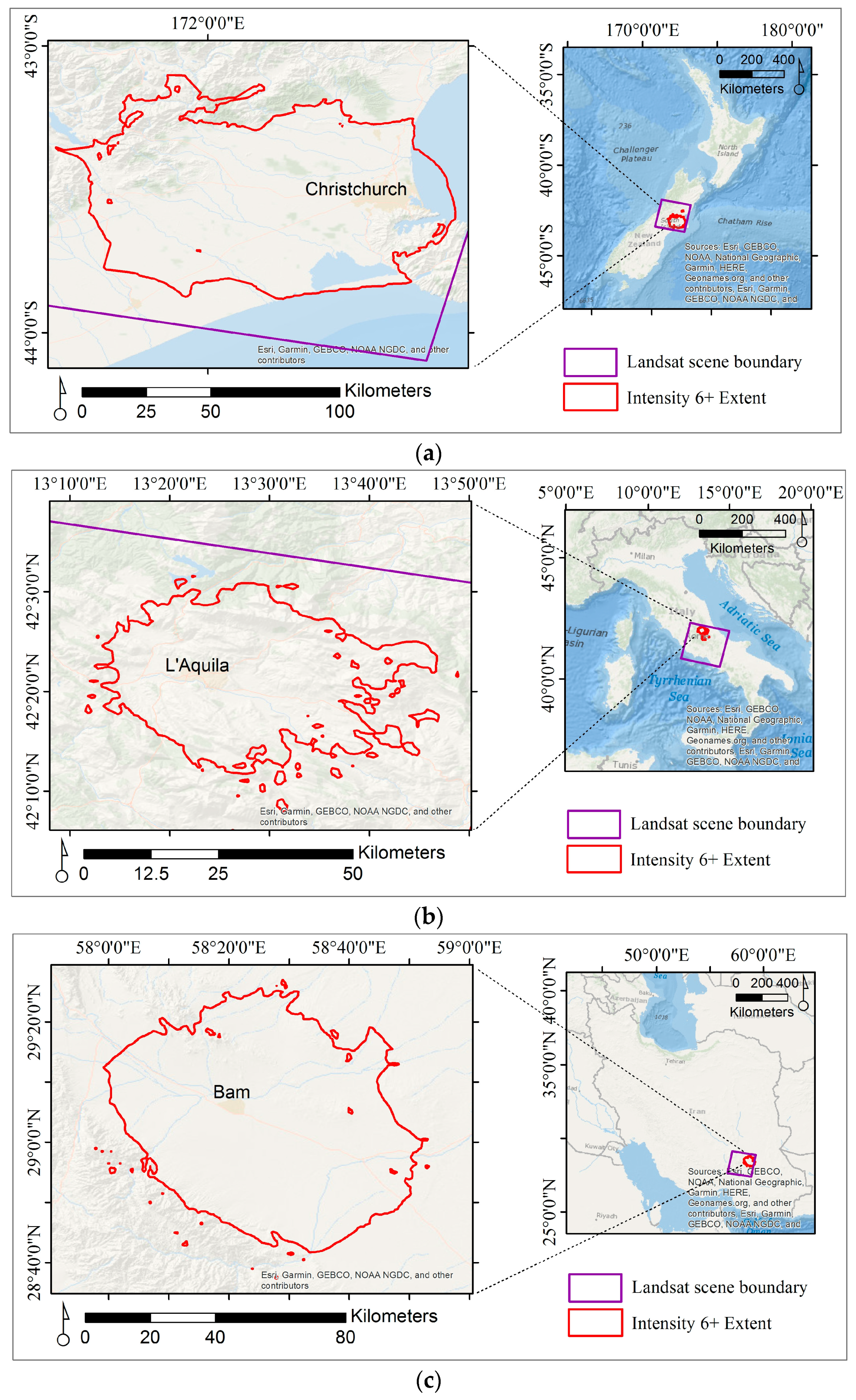
Three heterogeneous study areas were selected based on three earthquakes in different geographical locations across the globe: the Christchurch earthquake 2010 in New Zealand; the L’Aquila earthquake 2009 in Italy; and the Bam earthquake 2003 in Iran. The three selected events have distinctive recovery characteristics. On September 3, 2010 a M7.0 earthquake struck approximately 50 km to the west-northwest of Christchurch, New Zealand [49]. This mainshock (Canterbury earthquake) was followed by several aftershocks, including a M6.3 shock in 2011 (Christchurch earthquake). Consequently, 87% of homes in Christchurch were damaged (30% of them had major damage), more than 180 people died based on New Zealand’s police reports, and estimated damage from both shocks were about NZ$40 billion (2015$ value) according to the Reserve Bank of New Zealand [50,51]. The recovery encountered three to five year wait times for insurance claims payments, rezoning, and foundation standards [5]. On April 6, 2009, a M6.3 earthquake struck the city of L’Aquila, Italy [49]. As a result, 309 lost their lives, 1500 were injured, 3,000–10,000 buildings were damaged, and there was a total economic loss of EUR 17.4 billion (USD$ 20 billion, 2018$ value) according to Swiss Re estimates [52]. Within six months, the government built base isolated housing for 15,000 families. However, due to lack of funding, others lived in hotels and other towns for two to three years, and some relocated [5,53]. On December 26, 2003, an M6.6 earthquake struck city of Bam in southeastern Iran [49] that resulted in more than 26,000 loss of life, about 30,000 injuries, an estimated 70% complete loss of housing, and about USD$1.5 billion loss (2014$ value) from World Bank estimates [54,55].
All three earthquakes occurred in the time frame of 2000–2010 with Intensity > VIII and Magnitude > M6.0. The time frame of each case study starts from 10 years before the earthquake to present (2019). In this time frame, the pre-event and post-event imagery is collected. The 10 years of imagery before the earthquake is necessary for establishing a baseline estimate of the urban growth trend from pre-event conditions. Only urban areas are studied to monitor the urban/built-up land surface change before and after the event. The extent of area of interest (AOI) for each case is determined by the boundary of intensity of six (VI) or higher from USGS ShakeMap [49] (i.e., ‘slight damage’ or more based on Modified Mercalli intensity scale) for the earthquake events, since it delineates the possible region of physical damage (Figure 1).
The primary data in this study are Landsat imageries downloaded from USGS EarthExplorer (Landsat Collection Level 1) [56]. Table 1 below shows a summary of Landsat imagery used for the case studies (more details in Table 2). In order to find best time of image acquisition in certain year, the atmospheric conditions and phenology were examined. The environmental consideration of phenological cycle characteristics can be either for vegetation phenology or urban–suburban phenological cycles [57].
The images for each case are collected based on temporal availability, cloud coverage, and type of sensor availability. The 2003 Bam earthquake occurred at 5:26 am local time on 26 December and the months of January and February are chosen for anniversary date. The 2009 L’Aquila earthquake occurred on 6 April and the months of June and July are more suitable for anniversary dates due to cloud and snow coverage in other months. Lastly, the 2010 New Zealand occurred at 4:35 am local time on 4 September, 2010 with a major aftershock at 12:51 pm on 22 February 2011. The months of October and November are more suitable for anniversary dates but the actual dates of gathered imagery vary between Septembers to February due to cloud coverage. The time period between January–March is also in cyclone season. All these effects are taken into consideration when selecting the images. For initial analysis and data acquisition, there are no threshold assignments for cloud-coverage and the image that had the least cloud-coverage for each year is selected.
2.2. Methods
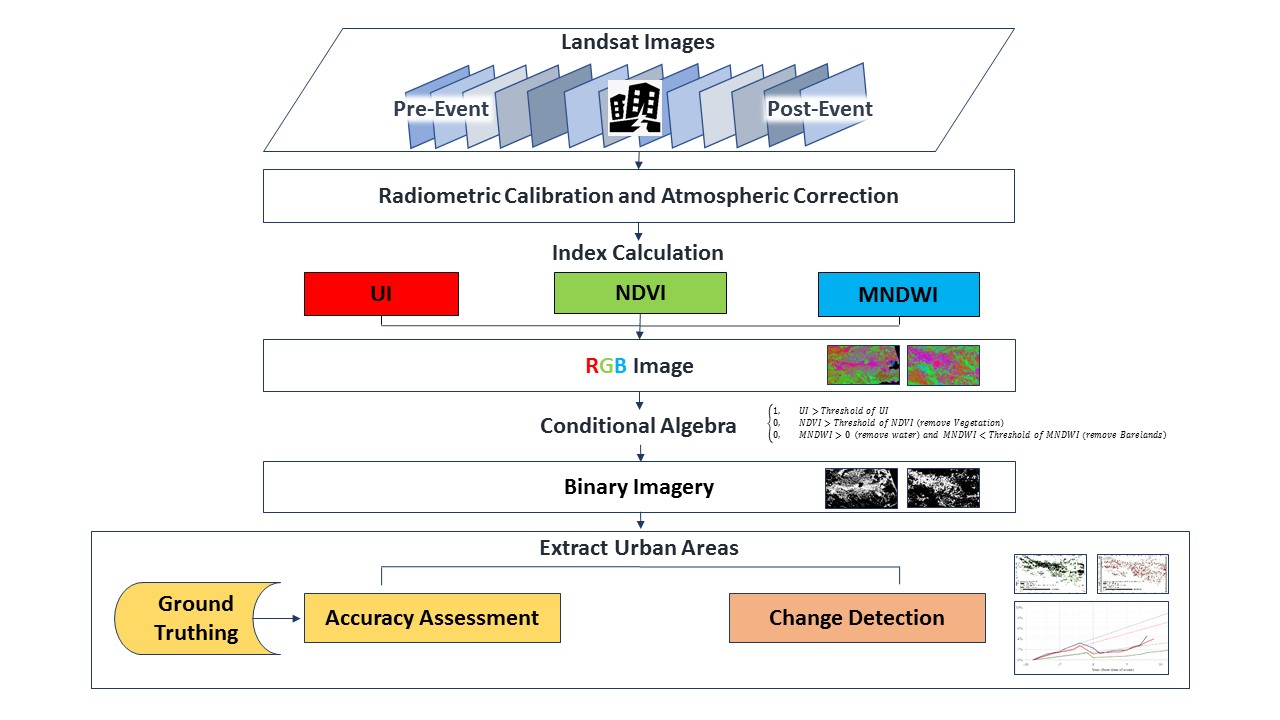
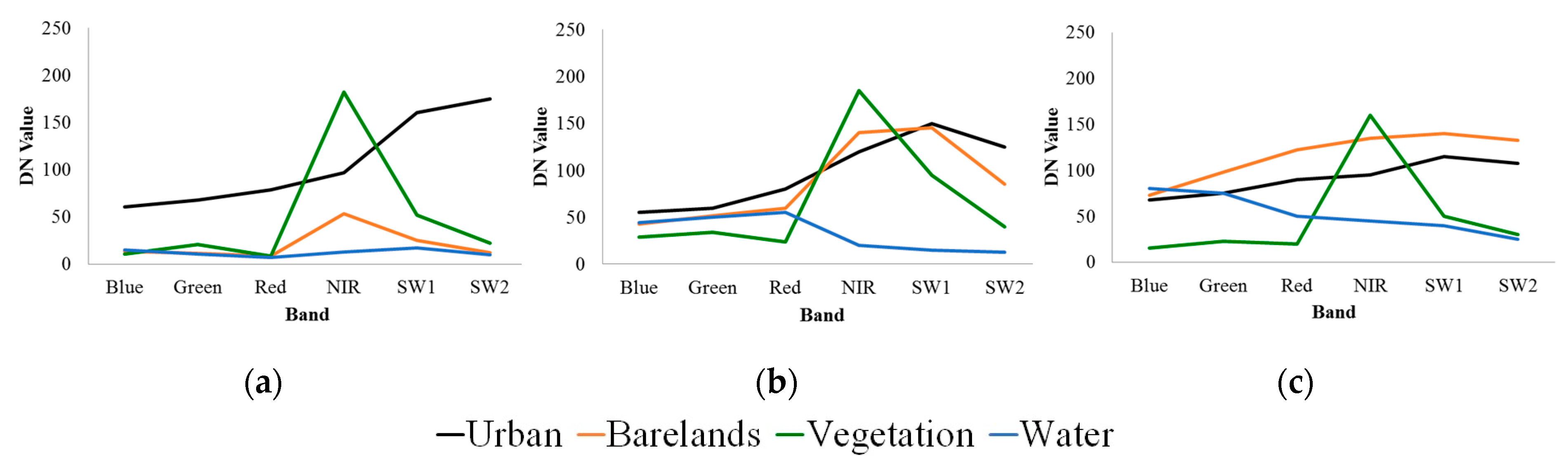
The proposed methodology uses three indices of UI, NDVI, and MNDWI, and builds a knowledge-based classifier to extract the urban/built-up features with a conditional algebra. These three indices are chosen after testing several combinations of indices that have shown reliable results based on literature and test sample points from three different years in each case (minimum 50 points/pixels randomly checked with high-resolution Google Earth images in AOI, for the same three years described in accuracy assessment) to delineate the built-up areas and remove the vegetation, water, and barelands. The spectral profiles for the sample points from the three cases is shown in Figure 2 that depicts the local variations and application of the three chosen indices as an average of spectral responses for each of the four classes. For example, the UI is preferred over other urban indices such as NDBI or EBBI since the distinction between urban/built-up areas versus barelands is better represented from the difference between SWIR2 and NIR, than SWIR1 and NIR (Figure 2b). Some complex urban indices, such as IBI, combine several bands but do not provide flexibility to include the local variations observed in our study cases and therefore, are not further investigated in this study. Hence, the UI is used to extract built-up surfaces, while NDVI is applied for removing vegetation and MNDWI is employed to eliminate both water-bodies and bareland. The formulas for the three indices are
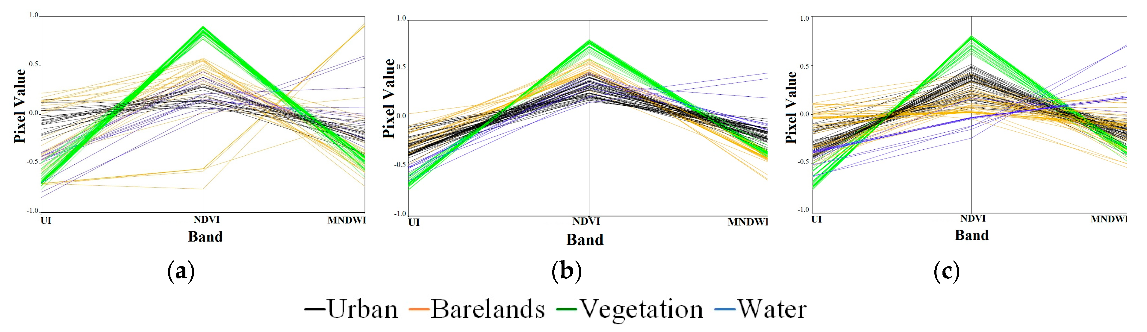
For each image, the three indices are calculated and composited into a three-layer RGB image: UI as Red, NDVI as Green, and MNDWI as Blue. This is the image used to classify urban/built-up and non-urban in this study. To extract built-up areas, a conditional algebraic test is applied to extract higher UI values and remove high NDVI and MNDWI values (Appendix A, Table A1). The Gaussian-based (Bayesian) automatic selection of thresholds for indices [58] was considered but due to the complexities of the urban landscape and earthquake cases, the pixel values do not follow a normal distribution. Also, as demonstrated with 100 randomly selected sample pixels in each case (Figure 3), urban index of built-up pixels reveals an extremely long range, reflecting heterogeneous urban structures. Brighter built-up pixels (higher UI values) are mixed with barelands, while the darker built-up pixels (lower UI values) could be mixed with some vegetation and water pixels. In the L’Aquila case (Figure 3b), UI values of built-up pixels are more densely clustered with barelands, even at higher UI values. In the Bam case (Figure 3c), UI values can better delineate built-up from barelands, but they show higher mixture with water. Figure 3 reveals that the UI itself could not optimally extract built-up pixels from barelands, vegetation, and water. On the other hand, vegetation is more distinguishable from NDVI, and water could be better identified from MNDWI. Therefore, a multi-index approach is established in this study. Figure 3 also shows the complexity of urban surface in different earthquake cases. Conditional algebra provided the means to assign optimal thresholds based on each case characteristics and variability of indices’ values that was especially effective in distinguishing barelands from built-up features. In the conditional statement, the threshold for high NDVI values removes vegetation and MNDWI is used to both remove both water bodies and the barelands, which is the reason that the conditional statement is applied to both higher values and lower values for this band. Since the histogram distributions are variable temporally and spatially, the thresholds start with a baseline defined based on literature [59,60,61], and the mean values for each band in each image to accommodate for the variability (Figure 3, Table 3). Finally, the classifier assigns each pixel from the three-layer image to a binary value of built-up/non-urban for each year. The general conditional statement for extracting built-up surfaces, prior to any modifications, is as below, (where 1 is indicating built-up and 0 is indicating non-urban):
The thresholds are different for each of the case studies due to the environmental, seasonal, and building variations. The variable phenological thresholds have been applied in past studies in analysis of NDVI time series [62]. In this study, Christchurch, New Zealand is in a flat area east of the Canterbury Plains and bounded by Pacific Ocean coast, volcanic slopes in the South and Waimakariri River in the North (Figure 3a); while the case of L’Aquila, Italy is mountainous (Figure 3b), and Bam is in a desert environment surrounded by mountains (Figure 3c). The values for a few cases are modified based on the histogram variation for the case and time of the year. It provides flexibility in defining the indices’ thresholds according to local characteristics, which enables more precise distinction of features based on environmental variability. Once classification is completed, the annual urban/built-up land surface change is calculated by subtracting the resulted binary pixel values of each year from its previous one.
A histogram match process is applied prior to index calculations. The imagery for a reference year is picked for histogram match based on having the least cloud coverage. For each case, all bands for all years are histogram matched by building a model in ERDAS Imagine. Hence, the inter-year variation from non-earthquake impacts such as atmospheric noises and weather are removed before extracting thresholds. The radiometric calibration and atmospheric correction is the first step in image processing, which is done by using the FLAASH (Fast Line-of-sight Atmospheric Analysis of Spectral Hypercubes) model in ENVI 5.4 software. Atmospheric correction is needed in this change detection method, since it is based on linear transformations of the data (e.g., NDVI) [54]. The FLAASH model incorporates the MODTRAN (MODerate spectral resolution atmospheric TRANsmittance) radiation transfer code to correct wavelengths in the visible through near-infrared and shortwave infrared regions [63]. If cloud coverage over the study area (AOI) was more that 10% of area for a year, those years were eliminated.
The accuracy assessment is the other part of methodology to estimate the rigor of classification results. The accuracy of classification is often reported as the percentage of correct identification, which is presented as errors of commission (presented as user’s accuracy referring to the percentage that are actually correct) and errors of omission (presented as the producer’s accuracy, is the percentage of the total pixels that belong to that category in the image). The confusion matrix is used with validation samples. The overall accuracy is calculated from the ratio of the sum of samples along the diagonal to the number of validation samples. In order to get representative random points for accuracy assessment, the number of points is selected by using a validation sample size for each case, and then they are distributed in two steps: 1) half of points are selected by equalized stratified random distribution that collects an equal number of random coordinates from each class; 2) the other half is a complete random distribution without replacement or any predefinitions. When accounting for the total number of pixels, with a 95% confidence level and confidence interval of 5, the minimum validation sample size is calculated for each case, which is rounded to 350 points for each case [56]. The random points are distributed in the pre-processed Landsat image and then compared with Google Earth satellite imagery and our classification.
3. Results
3.1. Conditional Algebra and Classification
The conditional algebra accommodates for local characteristics of each case with flexibility in defining the indices’ thresholds based on environmental and seasonal variability. Several thresholds were tested for each case and based on the statistics and standard deviation from the mean for each index values (Appendix A, Table A1), histogram distributions and sample testing points from both built-up and non-urban features (Figure 3), the best fitted thresholds were chosen that had higher accuracy percentages. The fitted thresholds are extracted from samples like Figure 3 for three years in each case and matched with the mean and standard deviation values of each index for the study area (appendix A), so that the conditional statement is only extracting urban features, and the thresholds are adjusted based on the histogram for that year. All thresholds are summarized in Table 3.
The example on (Figure 3a) indicates that lower MNDWI values show barelands and can provide a threshold to distinguish them from built-up lands. The threshold between these two at MNDWI in the sample points, is seen at −0.48, and after matching with MNDWI values for the whole study area with the mean of −0.456 and standard deviation of 0.135, the value of mean is a chosen threshold. This is tested for sample points from three other years for Christchurch, New Zealand and then applied for all years. The same process is applied for other indices as well (comparison of final results is presented in Figure 4). For each year, in case of New Zealand the thresholds were set based on
For each year, in case of Italy the thresholds are assigned as
The thresholds are set according to samples like Figure 3b, as it can be seen for example the lowest NDVI value seen in the sample is 0.48 for vegetation, and matching with general distribution of NDVI value for the study region in 2017, the mean is 0.588, and standard deviation of 0.133 (Appendix A, Table A1), thus threshold of one standard deviation below the mean matches a threshold for NDVI at value of 0.455 for 2017. The threshold is tested with similar samples from three years, and same process is applied for other indices. A comparison of final results is presented in Figure 5.
The Bam, Iran area, is surrounded by both desert (barelands) and mountains; therefore, the thresholds are slightly different from other cases to accommodate for the geographical features (Figure 3c) and only extract built-up areas based on the histograms. The lower threshold for NDVI in this case is helpful for eliminating barelands of surrounding desert (comparison of final results is presented in Figure 6). For each year, in the Iranian case the thresholds are assigned as
3.2. Accuracy Assessment
The Kappa coefficient of agreement is computed from the confusion matrix and reported for each case, in selected sample years. Due to large number of imagery and consistent methodology for each case, one representative image from every 10 years is chosen to simplify the assessment process. Hence, three sample years from the beginning, middle, and end of the time frame for each case study is chosen for accuracy assessment. The two classes that are extracted and presented in binary images are evaluated: built-up and non-urban.
According to the results (Table 4), the overall accuracy of urban/built-up ranges between 92% to 96.29%; and the Kappa value varies from 0.79 to 0.91. The lower user accuracy percentages for New Zealand 2017 and Italy 2017 are due to errors introduced from cloud presence, (even though the clouds are not over the AOI). Differences between sensors (TM versus OLI) do not seem to change the accuracy, as is seen in case of Iran. Thus, for longitudinal studies of large geographic areas, the proposed method provides the flexibility to delineate built-up land.
3.3. Change Detection
With the resulting class maps for each year, one application of the proposed methodology is change detection, which is tested for the three earthquake cases here. The change detection method is based on the differences in indices through years. In this method, the change from built-up to non-urban or the opposite is calculated in a yearly interval. The results show the annual spatial variations of urban/built-up surface change at pixel level, and summarized in Table 5. According to these results the estimated damage (% change from pre-event built-up area) is about 32% for Christchurch, 16% for L’Aquila, and about 63% for Bam (Table 5) that is close to the reports of extensive damages for these earthquakes. Also, results show that current built-up area is more than pre-event status in the study areas for Christchurch and L’Aquila, while total built-up area is still lower than pre-event for Bam. However, the annual growth trend can show the temporal dynamics of recovery process in these cases more in detail, thus, the results of urban land surface change are mapped for each case by pixels. In addition, the curves of percent urban land surface change for the study area are presented demonstrating the temporal trend. The maximum error detected from accuracy assessment for each case is included in the graphs to show the maximum extent of variability in the estimated urban land change. The years with imagery from Landsat 7 ETM+ after 31 May, 2003, (when the Scan Line Corrector (SLC) failed) are removed, since even the overlapped gap-filling images were introducing errors in change detection.
3.3.1. Case 1—Christchurch, New Zealand
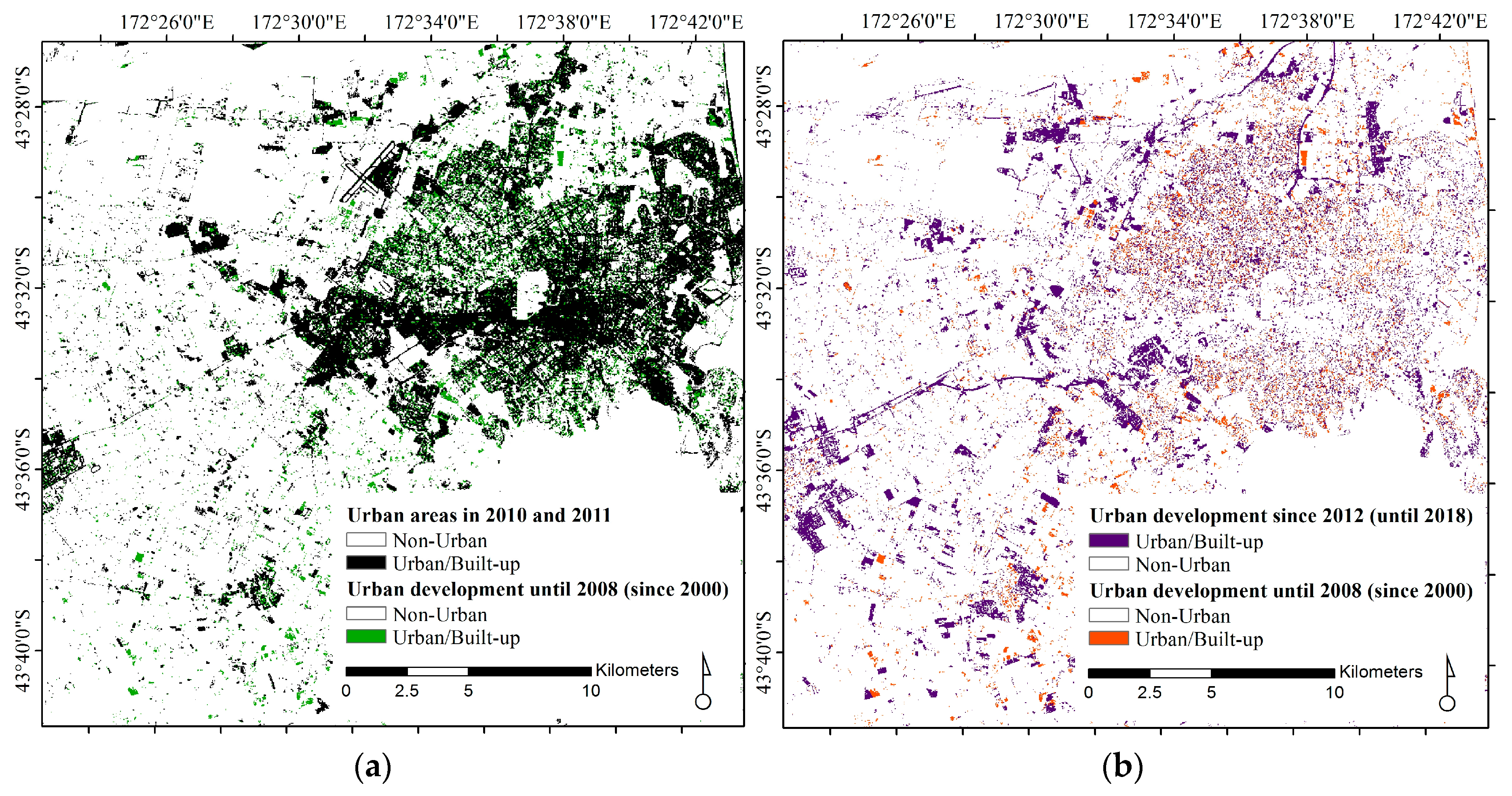
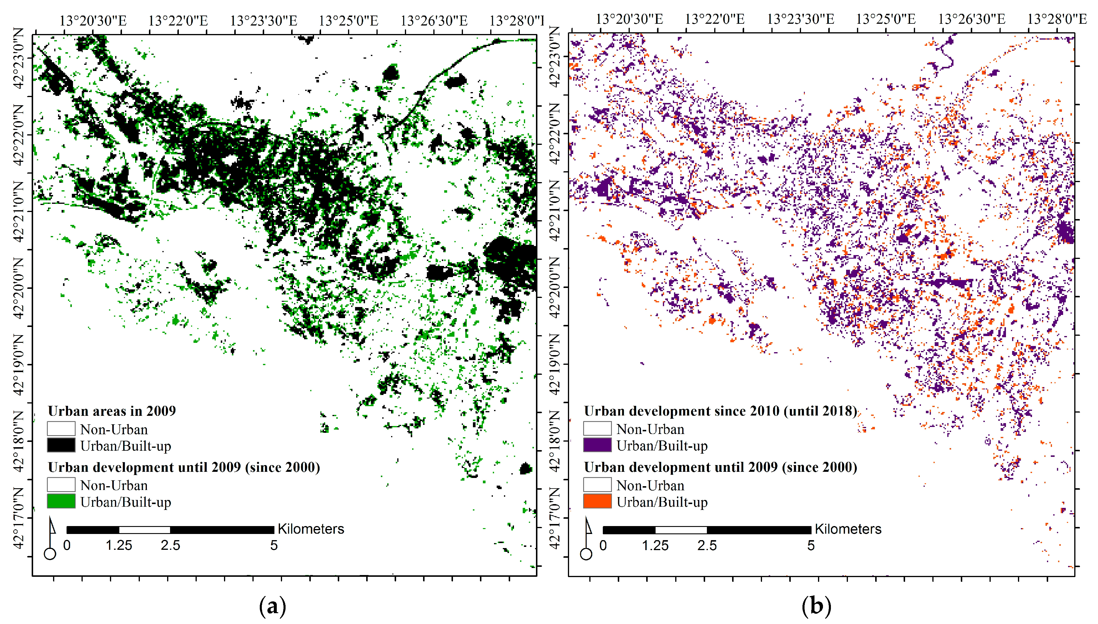
The map below show the areas detected as built-up/non-urban before and after the Christchurch earthquake and aftershock in New Zealand (Figure 7). The year of the earthquake and aftershock (2010 and 2011) is added in black, to visualize the change in urban area post-event (Figure 7a). The developments after the earthquake are displayed in purple after eliminating the built-up areas in 2010 and 2011 (i.e., not damaged) that show more construction and development in the western part of Christchurch and in Rolleston (Figure 7b). The orange areas show built-up lands from before the earthquakes, while some of the damaged area is reconstructed, some pockets have remained vacant, especially in the eastern parts, Central City and by the Avon River (marked as ‘Red Zones’ due to extensive damage from the liquefaction caused by the earthquake [64]).
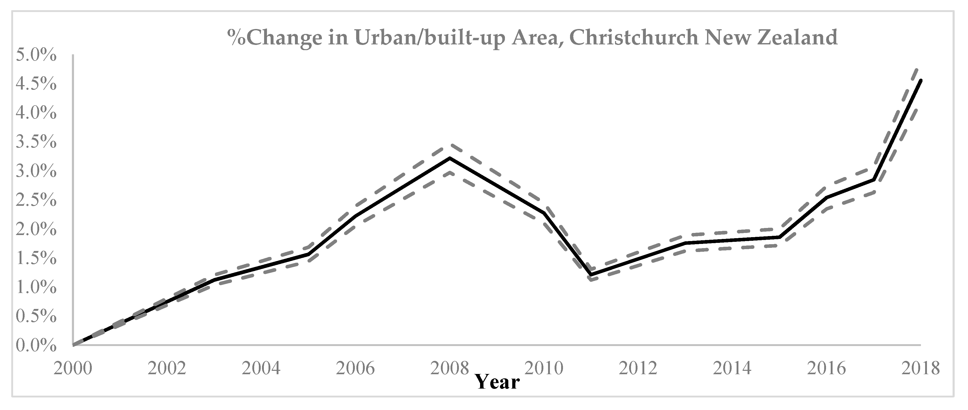
As is apparent from Figure 8, the urban/built-up land surface change rate in Christchurch is relatively constant before the 2010 earthquake, where there is a drop due to a negative change rate that extends to 2011 due to the aftershock and consequent damages. The change in trend appears to start after 2008, but it is due to the missing data point for 2009 (because of partial cloud coverage over urban lands in the 2009 image). The urban/built-up change trend continues positively after 2011 with a slower rate until 2015 and then shows a faster rate of urban growth.
3.3.2. Case 2—L’Aquila, Italy
The maps below show the areas near city of L’Aquila detected as built-up/non-urban for before and after the earthquake (Figure 9). The year of earthquake is added to visualize the change in urban area after the earthquake in black color (Figure 9a). The built-up area since 2010 is marked in purple and shows further development in the eastern part and some reconstruction near downtown areas (Figure 9b). The areas that remained as built-up are removed to only show new development in purple and the areas that have not been built back in orange. This shows that some areas in downtown have not been reconstructed yet.
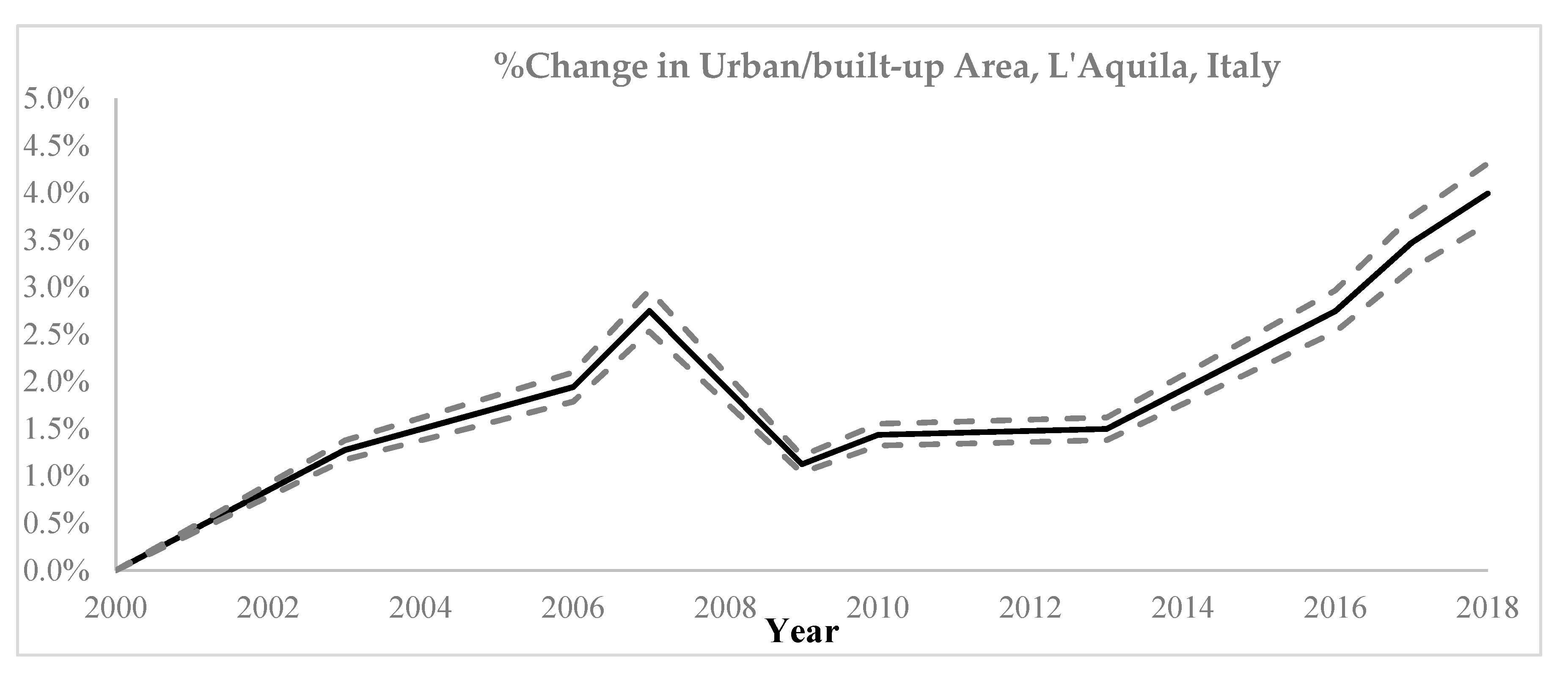
The curve of urban land surface change in L’Aquila is depicted in Figure 10 that shows the positive growth trend in urban/built-up area until 2007 and a drop in 2009 due to the earthquake damages. The 2008 image was removed because of cloud coverage on urban areas; hence there is no data point between 2007 and 2009. The urban/built-up change trend is relatively constant until 2013 and shows a growth trend afterwards.
3.3.3. Case 3—Bam, Iran
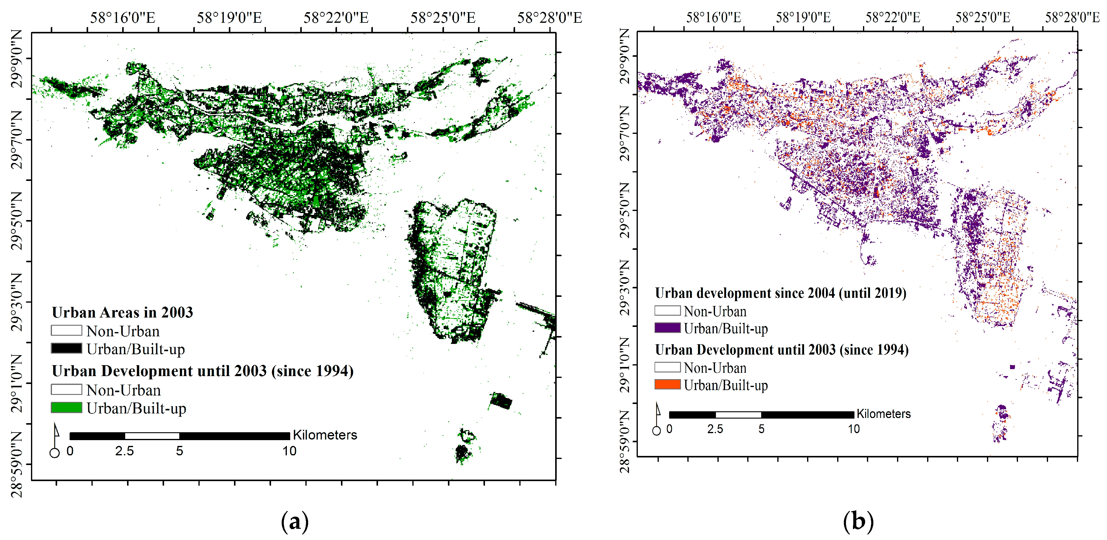
The maps below show the areas detected as built-up/non-urban for before and after the Bam earthquake, near city of Bam, Iran. The year of earthquake is added to visualize the change in urban area after the earthquake (Figure 11). The black areas represent undamaged and existing built-up surfaces after the earthquake in 2003 (Figure 11a), and the green areas show the pre-existing urban features that were not detected as built-up in 2003 (i.e., damaged or demolished). The areas that were not demolished in 2003 and remained built-up are subtracted from all years after the earthquake and presented in Figure 11b to show new development and remaining areas that have not been built back in orange. The purple areas are the newly developed built-up areas since 2004 (a year after the event), which show new constructions in the eastern and southern part of Bam.
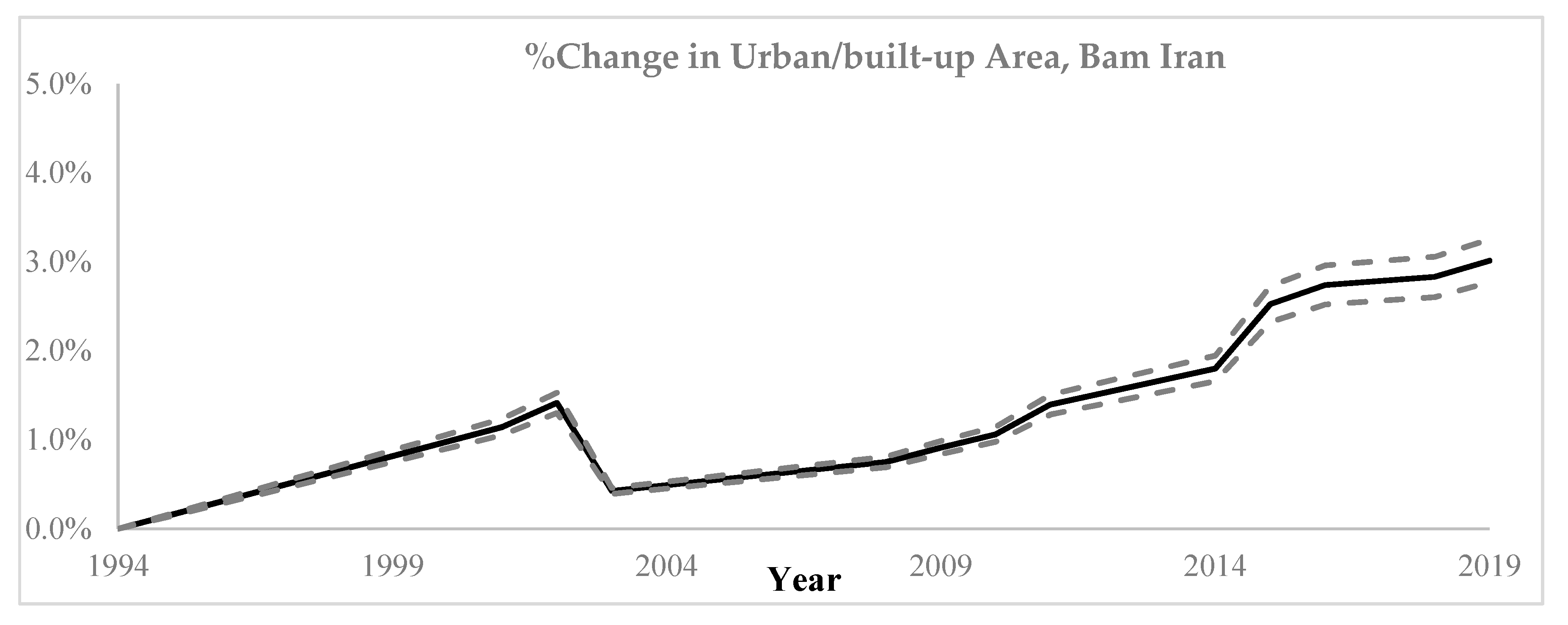
The urban/built-up land surface change in Bam is depicted in Figure 12 that shows a growth trend until 2003, which changes after the earthquake. The post-earthquake trend is rather constant until 2009 and shows growth until 2014, followed by an instant increase in growth rate until 2016 but then seems fairly constant until 2019.
The curves of percent urban/built-up area change depict the development and growth trend in the three cases. The pre-event imagery is helpful in defining a baseline for the development trend before the earthquake, while the post-event imagery shows how much the pre-event trend has been altered after the incident.
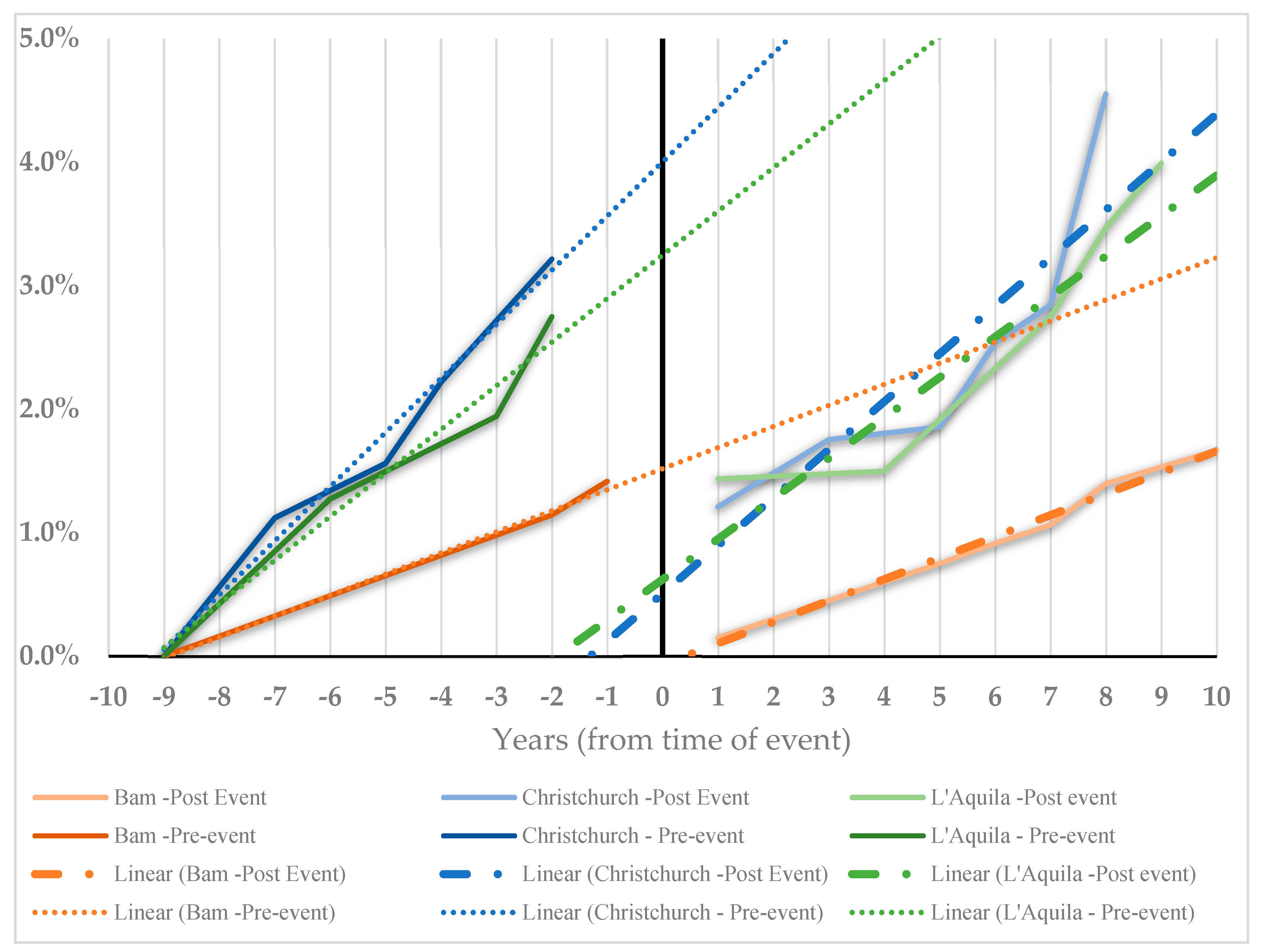
Figure 13 juxtaposes the land surface change trends together with additional linear forecast lines from pre-event data to demonstrate a comparative measure of how these communities are recovering according to the pre-existing development processes. The slopes of projected trends from pre-event data are 0.0044 for Christchurch, 0.0035 for L’Aquila, and 0.0016 for Bam; which can be compared with each segment of post-earthquake trends to see the relative recovery and development process for different time-frames. On the other hand, the projected trends from 10-years of post-event data, has a slope of 0.0039 for Christchurch, 0.0033 for L’Aquila, and 0.0017 for Bam. These pre-event versus post-event trends indicate that Bam has just surpassed the pre-event growth, while the other two cases have not reached their pre-event growth trends in a decadal comparison. However, the diversity in general growth trends for each case is observable in Figure 13, where Christchurch shows a higher growth speed (steeper slope) for both pre-event and post-event trends. Also, since recovery is a process, looking at specific time-windows can be an instrument for monitoring the recovery process for each case, based on the baseline that is specific to that case from their pre-event trends. For example, within the first 5 years after the earthquake in Christchurch (depicted by blue line in Figure 13) the slope is 0.0016, which is much less that the pre-event growth trend, but the time-window of 5-year to 10-years after the earthquake has a slope of 0.0084 that is more than its post-event decadal growth trend. In other words, the trend of built-up land growth in Bam is caught up with pre-event trend; however, the total built-up area is still lower than pre-event (Table 5), thus still recovering. In contrast, even though the decadal post-event growth trend is slacking in the other two cases, the growth trend in more recent years has surpassed the pre-event trends in Christchurch and just caught up with pre-event trends in L’Aquila, and they both have higher percentage of built-up area when compared to pre-event (Table 5). These comparable curves show the relative trend of urban change that will inform more details about the recovery process if combined with the socio-economic information. The observed differences in the trends need further investigation to find explanatory variables of such variations through time.
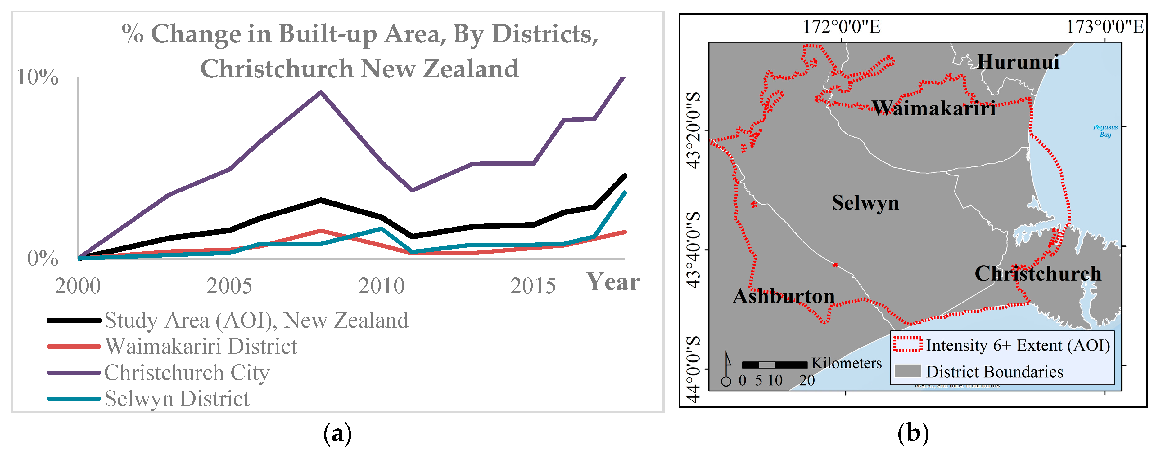
Depending on the extent of study, these results can be aggregated based on administrative boundaries to have the percent area change in urban surfaces for each administrative unit or neighborhood. A division of change trends by smaller administrative boundaries is specifically helpful in determining and comparing the location of new developments and reconstructions, since the total change trend for a large study area might be misleading as some neighborhoods might not been reconstructed or other new neighborhoods are developing that can be added to the analysis of recovery depending on the scale of study. For example, the percent built-up area change is summarized and presented by districts for the case of Christchurch, New Zealand (Figure 14). Since these curves depict the percentage of changes in the built-up area, the changes for Christchurch city district shows a higher level of change compared with the other regions in the study area. Even though the post-event growth trend for Christchurch city is slow until 2015 (slope of 0.0037), which is much lower than its pre-event trend with slope of 0.0111, it shows a steep increase after 2015 until 2018 with a slope of 0.0147 that has surpassed its pre-event values. Also noteworthy is the growth trend for the Selwyn District that shows a higher slope in the recent years (slope of 0.0046) when compared with pre-event trend for this district (slope of 0.0011). A ground truthing study can further validate or evaluate the quality of these estimations.
4. Discussion
The application of remote sensing for tracking urban land surface change in order to understand the reconstruction phase of the recovery process after a major disaster can inform decision makers for both recovery planning and resilience measurements. As indicated by the case studies’ results, the urban/built-up land surface change could be monitored with the proposed methodology, which can depict the development process and growth trend through time. Even though this method only applies to the changes in the physical built environment and not the socio-economic characteristics of the community, it has the potential to be combined with such data from other sources to provide a more holistic view of the recovery process. In our upcoming research, these measures are applied to a combination of both physical and socio-economic aspects for modeling a more comprehensive recovery process and gauging the relative success of the recovery.
The pre-event imagery is essential to decipher the disaster impact and recovery process, which requires establishing a database and image collection with designed temporal intervals for hazardous regions. Since official records of building and structures are not uniformly available in different regions and countries due to complexities of data collection and regulations, a repository of built environment imagery is a promising alternative to monitor the changes and allocate development resources appropriately. This would enable longitudinal studies of development trends that can be applied to studies other than disaster impacts as well. The importance of this method lies in establishing a baseline based on pre-existing conditions and growth trends in the community for a more realistic expectation of the temporal and spatial recovery trend. As it was seen in the three examples investigated in this study, the differential growth trends from pre-event to post-event provides a relative measure of recovery progress. Hence, application of this methodology for more cases will inform a comparative view of how communities recover through time after a disaster.
Moreover, the method provides the potential to aggregate the built-up surface change results with other layers of information about different indicators—such as the community traits and economic status, building materials, ground motion characteristics, hazard levels or damage status, etc.—for a more holistic view of the recovery process. The quality of rebuilding and reconstruction is missing in this method but can be achieved with ground truthing and field study. Clearly, higher resolution imagery can improve the results and precision of detecting the percent urban/built-up area change, and complement the results of this method. Additionally, the proposed method has flexibility in defining the thresholds with the conditional algebra statements according to local characteristics, which warrants more precise differentiation of features based on environmental variability. However, this flexibility introduces subjectivity in modifying the thresholds that is inevitable and more accurate in comparison with similar approaches. The logic calculation method has showed higher accuracy in similar cases, compared with a band spectral signature analysis, maximum likelihood supervised classification, or a principal component analysis (PCA), while being less subjective or time-consuming [60].
Future research directions would include application of higher spatial, spectral, and temporal resolution data to test the methodology and compare results. In addition, the results of this study can be juxtaposed with the object-based change detection models to further investigate their relative advantages and disadvantages. Finally, with larger number of images the machine learning methodologies would help processing more scenes and test the results for different geographical locations and contexts.
5. Conclusions
This study employs a conditional algebra in a knowledge-based classifier to extracts the urban/built-up features in three earthquake cases. Three spectral indices, UI, NDVI, and MNDWI, are used in the classifier. The results have an overall accuracy of 92% to 96.29%; and the Kappa value of 0.79 to 0.91 in three study cases.
The method’s flexibility in threshold definition with the conditional algebra statements accounts for local characteristics and distinction of features based on environmental variability, which also can be seen as the shortcoming of the method due to the subjectivity in modifying the thresholds. Regardless, the results indicated the potential of the proposed model in delineating the built-up surfaces that can provide essential information about the urban change trend when other sources of data are not available or accessible. Also, this method enables a relative measure of recovery that—once combined with variations in ground motion characteristics, building type distribution, and socio-economic data—allows a more holistic view of the recovery process. According to the findings from the three earthquake cases, total built-up area has increased in two cases of Christchurch and L’Aquila compared with pre-event area, which is also observed from the annual growth trend with a steeper rate in recent years. However, in case of Bam, when comparing recent years to pre-event years, the growth trend has the same rate as pre-event, but the total built-up area is still less than pre-event status. The spatial distribution of built-up area change in all three cases indicated that the post-earthquake developments are not necessarily on the damaged sites, and some areas have not been built back.
Lastly, the curves of percent urban/built-up area change provide a comparable overview of the development and growth trend post-earthquake in the affected regions. Hence, the utilization of annual imagery for detecting urban surface change can inform researchers and policy makers about the temporal and spatial nature of the recovery process and the impacts of the disaster. Application of this methodology for more cases will provide more insight on the observed disparities in the recovery process based on pre-existing trends before the disaster event, both temporally and spatially.
Author Contributions
S.D. designed the research, conducted image analysis, and finished the manuscript. S.L.C. assisted with finalizing the research framework; C.W. assisted with the methodological design. S.L.C. and C.W. contributed on reviewing and editing the final manuscript. All authors have read and agreed to the published version of the manuscript.
Funding
The publication of this research is supported by the Hazards and Vulnerability Research Institute (HVRI) and Department of Geography, at University of South Carolina, Columbia.
Acknowledgments
The authors acknowledge the support from the Hazards and Vulnerability Research Institute (HVRI), University of South Carolina for this research. The paper benefited from constructive discussions with Melanie Gall (from Arizona State University) and Zhenlong Li (from University of South Carolina), and three anonymous reviewers. Also, the first author is a recipient of Presidential Fellowship from graduate school of University of South Carolina and thanks them for the support during this study.
Conflicts of Interest
The authors declare no conflict of interest.
Appendix A

Table A1.
Summary statistics (mean, median, and standard deviation) for the constructed three-band images from UI, NDVI, and MNDWI, for each case study.
Table A1.
Summary statistics (mean, median, and standard deviation) for the constructed three-band images from UI, NDVI, and MNDWI, for each case study.
| New Zealand | |||||||||
| Year | Band | Mean | Median | S.Dev. | Year | Band | Mean | Median | S.Dev. |
| 2018 | UI | −0.39078 | −0.38586 | 0.239769 | 2008 | UI | −0.42607 | −0.43995 | 0.277791 |
| NDVI | 0.549269 | 0.554388 | 0.221035 | NDVI | 0.56676 | 0.605667 | 0.25924 | ||
| MNDWI | −0.44029 | −0.47534 | 0.129437 | MNDWI | −0.41125 | −0.47743 | 0.233257 | ||
| 2017 | UI | −0.41672 | −0.44451 | 0.214721 | 2007 | UI | −0.36858 | −0.3748 | 0.270372 |
| NDVI | 0.586788 | 0.60938 | 0.208631 | NDVI | 0.542433 | 0.550122 | 0.251433 | ||
| MNDWI | −0.45626 | −0.487 | 0.135116 | MNDWI | −0.45299 | −0.48928 | 0.148647 | ||
| 2016 | UI | −0.41213 | −0.43617 | 0.245014 | 2006 | UI | −0.41235 | −0.47716 | 0.287151 |
| NDVI | 0.561462 | 0.595593 | 0.24369 | NDVI | 0.583248 | 0.640979 | 0.268484 | ||
| MNDWI | −0.44339 | −0.47657 | 0.141168 | MNDWI | −0.45881 | −0.49348 | 0.146982 | ||
| 2015 | UI | −0.42061 | −0.45747 | 0.256856 | 2005 | UI | −0.40861 | −0.45492 | 0.26143 |
| NDVI | 0.574814 | 0.619058 | 0.2598 | NDVI | 0.580184 | 0.626747 | 0.250722 | ||
| MNDWI | −0.44317 | −0.47874 | 0.146284 | MNDWI | −0.4589 | −0.49152 | 0.13583 | ||
| 2014 | UI | −0.4214 | −0.46045 | 0.248374 | 2004 | UI | −0.43231 | −0.47848 | 0.299915 |
| NDVI | 0.577278 | 0.62252 | 0.247251 | NDVI | 0.606597 | 0.648942 | 0.262424 | ||
| MNDWI | −0.44033 | −0.48029 | 0.146544 | MNDWI | −0.46093 | −0.49075 | 0.20124 | ||
| 2013 | UI | −0.38415 | −0.40488 | 0.268944 | 2003 | UI | −0.44296 | −0.49574 | 0.255403 |
| NDVI | 0.540796 | 0.570015 | 0.25665 | NDVI | 0.586367 | 0.641341 | 0.248477 | ||
| MNDWI | −0.44253 | −0.47682 | 0.146363 | MNDWI | −0.43405 | −0.46628 | 0.141949 | ||
| 2011 | UI | −0.40134 | −0.42024 | 0.240505 | 2002 | UI | −0.43665 | −0.47856 | 0.251238 |
| NDVI | 0.563329 | 0.589227 | 0.227305 | NDVI | 0.58084 | 0.624461 | 0.242234 | ||
| MNDWI | −0.44802 | −0.48291 | 0.13939 | MNDWI | −0.44254 | −0.47884 | 0.140029 | ||
| 2010 | UI | −0.37024 | −0.36869 | 0.255088 | 2001 | UI | −0.4481 | −0.48869 | 0.250349 |
| NDVI | 0.538231 | 0.548401 | 0.241008 | NDVI | 0.593861 | 0.646662 | 0.235481 | ||
| MNDWI | −0.45525 | −0.49651 | 0.171679 | MNDWI | −0.43708 | −0.4692 | 0.138998 | ||
| 2009 | UI | −0.38958 | −0.38534 | 0.265487 | 2000 | UI | −0.42141 | −0.4481 | 0.2131 |
| NDVI | 0.548084 | 0.559005 | 0.22538 | NDVI | 0.586131 | 0.605933 | 0.209651 | ||
| MNDWI | −0.42047 | −0.467 | 0.203803 | MNDWI | −0.45596 | −0.48483 | 0.134306 | ||
| Italy | |||||||||
| Year | Band | Mean | Median | S.Dev. | Year | Band | Mean | Median | S.Dev. |
| 2018 | UI | −0.45988 | −0.47633 | 0.157215 | 2007 | UI | −0.46187 | −0.47441 | 0.155602 |
| NDVI | 0.575063 | 0.59461 | 0.139353 | NDVI | 0.581485 | 0.598339 | 0.136418 | ||
| MNDWI | −0.37912 | −0.39182 | 0.060955 | MNDWI | −0.37944 | −0.38948 | 0.058556 | ||
| 2017 | UI | −0.4699 | −0.47898 | 0.152075 | 2006 | UI | −0.46412 | −0.46783 | 0.152702 |
| NDVI | 0.588375 | 0.601054 | 0.132866 | NDVI | 0.5817 | 0.590286 | 0.134398 | ||
| MNDWI | −0.37511 | −0.39314 | 0.066702 | MNDWI | −0.3782 | −0.39207 | 0.064189 | ||
| 2016 | UI | −0.46298 | −0.47053 | 0.146413 | 2005 | UI | −0.47864 | −0.48554 | 0.14178 |
| NDVI | 0.581764 | 0.593306 | 0.128036 | NDVI | 0.587942 | 0.597798 | 0.127859 | ||
| MNDWI | −0.37981 | −0.39533 | 0.063622 | MNDWI | −0.37112 | −0.38805 | 0.069501 | ||
| 2014 | UI | −0.46494 | −0.48502 | 0.15578 | 2004 | UI | −0.48773 | −0.50949 | 0.155486 |
| NDVI | 0.583811 | 0.605026 | 0.13583 | NDVI | 0.606135 | 0.621044 | 0.126869 | ||
| MNDWI | −0.38142 | −0.39252 | 0.057668 | MNDWI | −0.38363 | −0.39062 | 0.060264 | ||
| 2013 | UI | −0.46248 | −0.47801 | 0.153945 | 2003 | UI | −0.45063 | −0.46467 | 0.16267 |
| NDVI | 0.581252 | 0.601237 | 0.137318 | NDVI | 0.573373 | 0.590863 | 0.140128 | ||
| MNDWI | −0.38055 | −0.39563 | 0.06243 | MNDWI | −0.37896 | −0.38899 | 0.062928 | ||
| 2011 | UI | −0.46797 | −0.47483 | 0.143414 | 2002 | UI | −0.48522 | −0.49819 | 0.120156 |
| NDVI | 0.590499 | 0.598766 | 0.122756 | NDVI | 0.607342 | 0.616981 | 0.10194 | ||
| MNDWI | −0.38632 | −0.39389 | 0.052889 | MNDWI | −0.3868 | −0.39611 | 0.049491 | ||
| 2010 | UI | −0.46023 | −0.47095 | 0.158986 | 2001 | UI | −0.46448 | −0.47073 | 0.153418 |
| NDVI | 0.579568 | 0.595716 | 0.139668 | NDVI | 0.579941 | 0.590647 | 0.135853 | ||
| MNDWI | −0.37981 | −0.39151 | 0.060715 | MNDWI | −0.37968 | −0.3933 | 0.061099 | ||
| 2009 | UI | −0.46042 | −0.46789 | 0.150657 | 2000 | UI | −0.46818 | −0.47318 | 0.148897 |
| NDVI | 0.579534 | 0.591728 | 0.132847 | NDVI | 0.586128 | 0.59645 | 0.132226 | ||
| MNDWI | −0.37871 | −0.39249 | 0.061825 | MNDWI | −0.37768 | −0.39329 | 0.063326 | ||
| 2008 | UI | −0.49747 | −0.50899 | 0.133064 | 1999 | UI | −0.46367 | −0.47284 | 0.148969 |
| NDVI | 0.623121 | 0.626003 | 0.104567 | NDVI | 0.582181 | 0.593583 | 0.130644 | ||
| MNDWI | −0.38934 | −0.40252 | 0.08009 | MNDWI | −0.37935 | −0.39402 | 0.065161 | ||
| Iran | |||||||||
| Year | Band | Mean | Median | S.Dev. | Year | Band | Mean | Median | S.Dev. |
| 2019 | UI | −0.11219 | −0.04443 | 0.186106 | 2008 | UI | −0.09019 | −0.0504 | 0.156866 |
| NDVI | 0.128086 | 0.044251 | 0.204314 | NDVI | 0.125936 | 0.050317 | 0.175914 | ||
| MNDWI | −0.17134 | −0.13379 | 0.108337 | MNDWI | −0.18724 | −0.13397 | 0.160179 | ||
| 2018 | UI | −0.10327 | −0.04279 | 0.162276 | 2003 | UI | −0.10195 | −0.0514 | 0.127771 |
| NDVI | 0.121296 | 0.045715 | 0.183081 | NDVI | 0.122557 | 0.051743 | 0.148494 | ||
| MNDWI | −0.16564 | −0.13324 | 0.087398 | MNDWI | −0.1697 | −0.1378 | 0.08242 | ||
| 2017 | UI | −0.11068 | −0.0415 | 0.193821 | 2002 | UI | −0.09909 | −0.05408 | 0.110781 |
| NDVI | 0.128723 | 0.044739 | 0.212135 | NDVI | 0.118094 | 0.05433 | 0.123516 | ||
| MNDWI | −0.17766 | −0.14014 | 0.13172 | MNDWI | −0.16734 | −0.14296 | 0.071104 | ||
| 2016 | UI | −0.10585 | −0.0423 | 0.18554 | 2001 | UI | −0.09907 | −0.05466 | 0.108117 |
| NDVI | 0.125799 | 0.044922 | 0.208824 | NDVI | 0.116164 | 0.053607 | 0.123499 | ||
| MNDWI | −0.17618 | −0.13666 | 0.131099 | MNDWI | −0.1644 | −0.13769 | 0.073891 | ||
| 2015 | UI | −0.11187 | −0.04852 | 0.173843 | 2000 | UI | −0.0836 | −0.05805 | 0.083978 |
| NDVI | 0.129628 | 0.049194 | 0.193488 | NDVI | 0.096814 | 0.056358 | 0.08859 | ||
| MNDWI | −0.17093 | −0.13245 | 0.10634 | MNDWI | −0.15652 | −0.14078 | 0.054048 | ||
| 2014 | UI | −0.10044 | −0.04668 | 0.14641 | 1998 | UI | −0.10356 | −0.05139 | 0.160863 |
| NDVI | 0.115963 | 0.047983 | 0.165636 | NDVI | 0.113833 | 0.050293 | 0.175388 | ||
| MNDWI | −0.16109 | −0.13142 | 0.079309 | MNDWI | −0.16304 | −0.13251 | 0.105557 | ||
| 2013 | UI | −0.08814 | −0.0422 | 0.158923 | 1997 | UI | −0.10127 | −0.05066 | 0.160451 |
| NDVI | 0.125114 | 0.045073 | 0.180592 | NDVI | 0.110876 | 0.046997 | 0.173173 | ||
| MNDWI | −0.18785 | −0.13675 | 0.15265 | MNDWI | −0.15972 | −0.13007 | 0.102911 | ||
| 2011 | UI | −0.10842 | −0.05463 | 0.158138 | 1996 | UI | −0.06614 | −0.04301 | 0.092433 |
| NDVI | 0.116651 | 0.051697 | 0.17135 | NDVI | 0.070858 | 0.040804 | 0.099626 | ||
| MNDWI | −0.15785 | −0.13208 | 0.08638 | MNDWI | −0.13408 | −0.11909 | 0.055691 | ||
| 2010 | UI | −0.1005 | −0.04729 | 0.153095 | 1995 | UI | −0.09722 | −0.05527 | 0.112364 |
| NDVI | 0.116022 | 0.049744 | 0.173604 | NDVI | 0.113067 | 0.054428 | 0.132811 | ||
| MNDWI | −0.16589 | −0.13641 | 0.095609 | MNDWI | −0.16446 | −0.13516 | 0.082296 | ||
| 2009 | UI | −0.10061 | −0.04877 | 0.159913 | 1994 | UI | −0.096 | −0.0539 | 0.115124 |
| NDVI | 0.11316 | 0.051514 | 0.170581 | NDVI | 0.11178 | 0.050387 | 0.136184 | ||
| MNDWI | −0.16579 | −0.13696 | 0.100689 | MNDWI | −0.16062 | −0.13304 | 0.082763 | ||
References
- Quarantelli, E.L. What is a Disaster? Routledge: New York, NY, USA, 1998. [Google Scholar]
- Rubin, C.B.; Barbee, D.G. Disaster Recovery and Hazard Mitigation: Bridging the Intergovernmental Gap. Public Adm. Rev. 1985, 45, 57. [Google Scholar] [CrossRef] [Green Version]
- Bolin, R.C. Disaster impact and recovery: A comparison of black and white victims. Int. J. Mass Emergencies Disasters 1986, 4, 35–50. [Google Scholar]
- Olshansky, R.B.; Hopkins, L.D.; Johnson, L.A. Disaster and recovery: Processes compressed in time. Nat. Hazards Rev. 2012, 13, 173–178. [Google Scholar] [CrossRef]
- Comerio, M.C. Disaster recovery and community renewal: Housing approaches. Cityscape 2014, 16, 51–68. [Google Scholar]
- Cutter, S.L.; Emrich, C.T.; Mitchell, J.T.; Piegorsch, W.W.; Smith, M.M.; Weber, L. Hurricane Katrina and the Forgotten Coast of Mississippi; Cambridge University Press: Cambridge, UK, 2014. [Google Scholar]
- Oliver-Smith, A. Conversations in catastrophe: Neoliberalism and the cultural construction of disaster risk. In Cultures and Disasters: Understanding Cultural Framings in Disaster Risk Reduction; Routledge: New York, NY, USA, 2015; Chapter 2. [Google Scholar]
- Sarabandi, P.; Kiremidjian, A.S.; Eguchi, R.T.; Adams, B.J. Building Inventory Compilation for Disaster Management: Application of Remote Sensing and Statistical Modeling; Technical Report MCEER-08-0025; University at Buffalo: Buffalo, NY, USA, 2008. [Google Scholar]
- Duda, K.A.; Jones, B.K. USGS Remote Sensing Coordination for the 2010 Haiti Earthquake. Photogramm. Eng. Remote Sens. 2011, 77, 899–907. [Google Scholar] [CrossRef]
- Dellacqua, F.; Gamba, P. Remote Sensing and Earthquake Damage Assessment: Experiences, Limits, and Perspectives. Proc. IEEE 2012, 100, 2876–2890. [Google Scholar] [CrossRef]
- Tong, X.; Hong, Z.; Liu, S.; Zhang, X.; Xie, H.; Li, Z.; Yang, S.; Wang, W.; Bao, F. Building-damage detection using pre- and post-seismic high-resolution satellite stereo imagery: A case study of the May 2008 Wenchuan earthquake. ISPRS J. Photogramm. Remote Sens. 2012, 68, 13–27. [Google Scholar] [CrossRef]
- Bello, O.M.; Aina, Y.A. Satellite Remote Sensing as a Tool in Disaster Management and Sustainable Development: Towards a Synergistic Approach. Procedia-Soc. Behav. Sci. 2014, 120, 365–373. [Google Scholar] [CrossRef] [Green Version]
- Bevington, J.S.; Eguchi, R.T.; Gill, S.; Ghosh, S.; Huyck, C.K. A Comprehensive Analysis of Building Damage in the 2010 Haiti Earthquake Using High-Resolution Imagery and Crowdsourcing. Time-Sensitive Remote Sens 2015, 131–145. [Google Scholar] [CrossRef]
- Menderes, A.; Erener, A.; Sarp, G. Automatic Detection of Damaged Buildings after Earthquake Hazard by Using Remote Sensing and Information Technologies. Procedia Earth Planet. Sci. 2015, 15, 257–262. [Google Scholar] [CrossRef] [Green Version]
- Voigt, S.; Giulio-Tonolo, F.; Lyons, J.; Kučera, J.; Jones, B.; Schneiderhan, T.; Guha-Sapir, D. Global trends in satellite-based emergency mapping. Science 2016, 353, 247–252. [Google Scholar] [CrossRef] [PubMed]
- Ghaffarian, S.; Kerle, N.; Filatova, T. Remote Sensing-Based Proxies for Urban Disaster Risk Management and Resilience: A Review. Remote Sens. 2018, 10, 1760. [Google Scholar] [CrossRef] [Green Version]
- Kerle, N.; Ghaffarian, S.; Nawrotzki, R.; Leppert, G.; Lech, M. Evaluating Resilience-Centered Development Interventions with Remote Sensing. Remote Sens. 2019, 11, 2511. [Google Scholar] [CrossRef] [Green Version]
- Nex, F.; Duarte, D.; Steenbeek, A.; Kerle, N. Towards Real-Time Building Damage Mapping with Low-Cost UAV Solutions. Remote Sens. 2019, 11, 287. [Google Scholar] [CrossRef] [Green Version]
- Dopido, I.; Li, J.; Gamba, P.; Plaza, A. A New Hybrid Strategy Combining Semisupervised Classification and Unmixing of Hyperspectral Data. IEEE J. Sel. Top. Appl. Earth Obs. Remote Sens. 2014, 7, 3619–3629. [Google Scholar] [CrossRef]
- Jia, M.M.; Zhang, Y.Z.; Wang, Z.M.; Song, K.S.; Ren, C.Y. Mapping the Distribution of Mangrove Species in the Core Zone of Mai Po Marshes Nature Reserve, Hong Kong, Using Hyperspectral Data and High-Resolution Data. Int. J. Appl. Earth Obs. Geoinf. 2014, 33, 226–231. [Google Scholar] [CrossRef]
- Powers, R.P.; Hermosilla, T.; Coops, N.C.; Chen, G. Remote Sensing and Object-Based Techniques for Mapping Fine-Scale Industrial Disturbances. Int. J. Appl. Earth Obs. Geoinf. 2015, 34, 51–57. [Google Scholar] [CrossRef]
- Prosper, W.; Balz, T.; Mohamadi, B. Coherence Change-Detection with Sentinel-1 for Natural and Anthropogenic Disaster Monitoring in Urban Areas. Remote Sens. 2018, 10, 1026. [Google Scholar] [CrossRef] [Green Version]
- Gomez-Chova, L.; Fernandez-Prieto, D.; Calpe, J.; Soria, E.; Vila, J.; Camps-Valls, G. Urban monitoring using multi-temporal SAR and multi-spectral data. Pattern Recogn. Lett. 2006, 27, 234–243. [Google Scholar] [CrossRef]
- Ward, D.; Phinn, S.R.; Murray, A.T. Monitoring Growth in Rapidly Urbanizing Areas Using Remotely Sensed Data. Prof. Geogr. 2000, 52, 371–386. [Google Scholar] [CrossRef]
- Yang, X.; Lo, C.P. Using a Time Series of Satellite Imagery to Detect Land Use and Land Cover Changes in the Atlanta, Georgia Metropolitan Area. Int. J. Remote Sens. 2002, 23, 1775–1798. [Google Scholar] [CrossRef]
- Zhang, Q.; Wang, J.; Peng, X.; Gong, P.; Shi, P. Urban Built-up Land Change Detection with Road Density and Spectral Information from Multi-Temporal Landsat TM Data. Int. J. Remote Sens. 2002, 23, 3057–3078. [Google Scholar] [CrossRef]
- Sexton, J.O.; Song, X.-P.; Huang, C.; Channan, S.; Baker, M.E.; Townshend, J.R. Corrigendum to Urban Growth of the Washington, D.C.–Baltimore, MD Metropolitan Region from 1984 to 2010 by Annual, Landsat-Based Estimates of Impervious Cover. [Remote Sens. Environ. 2013, 129, 42–53.]. Remote Sens. Environ. 2014, 155, 379. [Google Scholar] [CrossRef]
- Li, X.; Gong, P.; Liang, L. A 30-Year (1984–2013) Record of Annual Urban Dynamics of Beijing City Derived from Landsat Data. Remote Sens. Environ. 2015, 166, 78–90. [Google Scholar] [CrossRef]
- Faridatul, M.I.; Wu, B. Automatic Classification of Major Urban Land Covers Based on Novel Spectral Indices. ISPRS Int. J. Geo-Inf. 2018, 7, 453. [Google Scholar] [CrossRef] [Green Version]
- Mas, J.F.; Velazquez, A.; Gallegos, J.R.D.; Saucedo, R.M.; Alcantare, C.; Bocco, G.; Castro, R.; Fernandez, T.; Vega, A.P. Assessing land use/cover changes: A nationwide multidate spatial database for Mexico. Int. J. Appl. Earth Obs. Geoinf. 2004, 5, 249–261. [Google Scholar] [CrossRef]
- Zhao, G.X.; Lin, G.; Warner, T. Using ThematicMapper data for change detection and sustainable use of cultivated land: A case study in the Yellow River delta, China. Int. J. Remote Sens. 2004, 25, 2509–2522. [Google Scholar] [CrossRef]
- Zewdie, W.; Csaplovies, E. Remote Sensing based multi- temporal land cover classification and change detection in northwestern Ethiopia. Eur. J. Remote Sens. 2015, 48, 121–139. [Google Scholar] [CrossRef] [Green Version]
- Ayele, G.T.; Tebeje, A.K.; Demissie, S.S.; Belete, M.A.; Jemberrie, M.A.; Teshome, W.M.; Teshale, E.Z. Time Series Land Cover Mapping and Change Detection Analysis Using Geographic Information System and Remote Sensing, Northern Ethiopia. Air Soil Water Res. 2018, 11. [Google Scholar] [CrossRef] [Green Version]
- Duro, D.C.; Franklin, S.E.; Dubé, M.G. A Comparison of Pixel-Based and Object-Based Image Analysis with Selected Machine Learning Algorithms for the Classification of Agricultural Landscapes Using SPOT-5 HRG Imagery. Remote Sens. Environ. 2012, 118, 259–272. [Google Scholar] [CrossRef]
- Al-Khudhairy, D.H.A.; Caravaggi, I.; Giada, S. Structural Damage Assessments from Ikonos Data Using Change Detection, Object-Oriented Segmentation, and Classification Techniques. Photogramm. Eng. Remote Sens. 2005, 71, 825–837. [Google Scholar] [CrossRef] [Green Version]
- Myint, S.W.; Gober, P.; Brazel, A.; Grossman-Clarke, S.; Weng, Q. Per-Pixel vs. Object-Based Classification of Urban Land Cover Extraction Using High Spatial Resolution Imagery. Remote Sens. Environ. 2011, 115, 1145–1161. [Google Scholar] [CrossRef]
- De Alwis Pitts, D.A.; So, E. Enhanced Change Detection Index for Disaster Response, Recovery Assessment and Monitoring of Buildings and Critical Facilities—A Case Study for Muzzaffarabad, Pakistan. Int. J. Appl. Earth Obs. Geoinf. 2017, 63, 167–177. [Google Scholar] [CrossRef]
- Varshney, A. Improved NDBI Differencing Algorithm for Built-up Regions Change Detection from Remote-Sensing Data: An Automated Approach. Remote Sens. Lett. 2013, 4, 504–512. [Google Scholar] [CrossRef]
- Valdiviezo-N, J.C.; Téllez-Quiñones, A.; Salazar-Garibay, A.; López-Caloca, A.A. Built-up Index Methods and Their Applications for Urban Extraction from Sentinel 2A Satellite Data: Discussion. J. Opt. Soc. Am. 2017, 35, 35. [Google Scholar] [CrossRef] [PubMed]
- Kawamura, M.; Jayamana, S.; Tsujiko, Y. Relation between social and environmental conditions in Colombo Sri Lanka and the Urban Index estimated by satellite remote sensing data. Int. Arch. Photogramm. Remote Sens. 1996, 31, 321–326. [Google Scholar]
- Zha, Y.; Gao, J.; Ni, S. Use of Normalized Difference Built-up Index in Automatically Mapping Urban Areas from TM Imagery. Int. J. Remote Sens. 2003, 24, 583–594. [Google Scholar] [CrossRef]
- He, C.; Shi, P.; Xie, D.; Zhao, Y. Improving the Normalized Difference Built-up Index to Map Urban Built-up Areas Using a Semiautomatic Segmentation Approach. Remote Sens. Lett. 2010, 1, 213–221. [Google Scholar] [CrossRef] [Green Version]
- Xu, H. A New Index for Delineating Built-up Land Features in Satellite Imagery. Int. J. Remote Sens. 2008, 29, 4269–4276. [Google Scholar] [CrossRef]
- As-Syakur, A.R.; Adnyana, I.; Arthana, I.W.; Nuarsa, I.W. Enhanced Built-Up and Bareness Index (EBBI) for mapping built-up and bare land in an urban area. Remote Sens 2012, 4, 2957–2970. [Google Scholar] [CrossRef] [Green Version]
- Sinha, P.; Verma, N.K.; Ayele, E. Urban Built-up Area Extraction and Change Detection of Adama Municipal Area Using Time-Series Landsat Images. Int. J. Adv. Remote Sens. Gis. 2016, 5, 1886–1895. [Google Scholar] [CrossRef]
- Waqar, M.M.; Mirza, J.F.; Mumtaz, R.; Hussain, E. Development of New Indices for Extraction of Built-Up Area & Bare Soil from Landsat Data. Sci. Rep. 2012, 1, 136. [Google Scholar] [CrossRef]
- Li, H.; Wang, C.; Zhong, C.; Su, A.; Xiong, C.; Wang, J.; Liu, J. Mapping Urban Bare Land Automatically from Landsat Imagery with a Simple Index. Remote Sens. 2017, 9, 249. [Google Scholar] [CrossRef] [Green Version]
- Wieland, M.; Pittore, M. Performance Evaluation of Machine Learning Algorithms for Urban Pattern Recognition from Multi-Spectral Satellite Images. Remote Sens. 2014, 6, 2912–2939. [Google Scholar] [CrossRef] [Green Version]
- U.S. Geological Survey (USGS) Earthquake Hazards Program. Available online: https://earthquake.usgs.gov/earthquakes/eventpage/ (accessed on 20 January 2020).
- New Zealand Police Publication of Earthquake Fatalities 2011. Available online: http://www.police.govt.nz/sites/default/files/publications/christchurch-earthquake-fatalities-locations-map.pdf (accessed on 20 January 2020).
- Reserve Bank of New Zealand (February 2016), Bulletin, Volume 79, No. 3. Available online: https://www.rbnz.govt.nz/-/media/ReserveBank/Files/Publications/Bulletins/2016/2016feb79-3.pdf (accessed on 16 February 2020).
- Swiss Re Institute. Special feature for sigma No.2/2019. L’Aquila, 10 years on. 2019. Available online: https://www.swissre.com/dam/jcr:a1800651-558e-403a-b8df-cb4d8ce9e2ec/Sigma_2_2019_feature_EN.PDF (accessed on 16 February 2020).
- Contreras, D.; Blaschke, T.; Kienberger, S.; Zeil, P. Spatial connectivity as a recovery process indicator: The L’Aquila earthquake. Technol. Forecast. Soc. Chang. 2013, 80, 1782–1803. [Google Scholar] [CrossRef] [Green Version]
- Tierney, K.J.; Oliver-Smith, A. Social dimensions of disaster recovery. Int. J. Mass Emergencies Disasters 2012, 30, 123–146. [Google Scholar]
- The World Bank. Iran- Bam Earthquake Emergency Response Project (English); World Bank: Washington, DC, USA, 2004; Available online: http://documents.worldbank.org/curated/en/462231468284376813/Iran-Bam-Earthquake-Emergency-Response-Project (accessed on 16 February 2020).
- United States Geological Survey (USGS), EarthExplorer. Landsat Satellite Missions. Available online: https://earthexplorer.usgs.gov/ (accessed on 15 September 2019).
- Jensen, J.R. Introductory Digital Image Processing: A Remote Sensing Perspective, 4th ed.; Pearson Education Inc.: London, UK, 2016. [Google Scholar]
- Sun, Z.; Wang, C.; Guo, H.; Shang, R. A Modified Normalized Difference Impervious Surface Index (MNDISI) for Automatic Urban Mapping from Landsat Imagery. Remote Sens. 2017, 9, 942. [Google Scholar] [CrossRef] [Green Version]
- Roderick, M.; Smith, R.; Cridland, S. The Precision of the NDVI Derived from AVHRR Observations. Remote Sens. Environ. 1996, 56, 57–65. [Google Scholar] [CrossRef]
- Xu, H. Extraction of Urban Built-up Land Features from Landsat Imagery Using a Thematicoriented Index Combination Technique. Photogramm. Eng. Remote Sens. 2007, 73, 1381–1391. [Google Scholar] [CrossRef] [Green Version]
- Emanuele, M.; Bitelli, G. Multi-Image and Multi-Sensor Change Detection for Long-Term Monitoring of Arid Environments With Landsat Series. Remote Sens. 2015, 7, 14019–14038. [Google Scholar] [CrossRef] [Green Version]
- Wang, C.; Hunt, E.R.; Zhang, L.; Guo, H. Phenology-Assisted Classification of C3 and C4 Grasses in the U.S. Great Plains and Their Climate Dependency with MODIS Time Series. Remote Sens. Environ. 2013, 138, 90–101. [Google Scholar] [CrossRef]
- Anderson, G.P.; Pukall, B.; Allred, C.L.; Jeong, L.S.; Hoke, M.; Chetwynd, J.H.; Adler-Golden, S.M. FLAASH and MODTRAN4: State-of-the-Art Atmospheric Correction for Hyperspectral Data. In Proceedings of the 1999 IEEE Aerospace Conference, Proceedings (Cat. No.99TH8403), Snowmass at Aspen, CO, USA, 7 March 1999. [Google Scholar]
- Johnson, L.A.; Olshansky, R.B. After Great Disasters: An in-Depth Analysis of How Six Countries Managed Community Recovery; Lincoln Institute of Land Policy: Cambridge, MA, USA, 2017. [Google Scholar]
Figure 1.
Area of interest (AOI) for each case with the boundary of selected Landsat Scene. (a) Christchurch, New Zealand; (b) L’Aquila, Italy; (c) Bam, Iran (Basemap Source: Esri 2020).
Figure 1.
Area of interest (AOI) for each case with the boundary of selected Landsat Scene. (a) Christchurch, New Zealand; (b) L’Aquila, Italy; (c) Bam, Iran (Basemap Source: Esri 2020).

Figure 2.
Spectral profiles of four classes in (a) Christchurch, New Zealand; (b) L’Aquila, Italy; and (c) Bam, Iran.
Figure 2.
Spectral profiles of four classes in (a) Christchurch, New Zealand; (b) L’Aquila, Italy; and (c) Bam, Iran.

Figure 3.
Spectral profiles of four classes in the constructed RGB images for 100 random sample pixels in (a) Christchurch, New Zealand (2017); (b) L’Aquila, Italy (2017); and (c) Bam, Iran (2018).
Figure 3.
Spectral profiles of four classes in the constructed RGB images for 100 random sample pixels in (a) Christchurch, New Zealand (2017); (b) L’Aquila, Italy (2017); and (c) Bam, Iran (2018).

Figure 4.
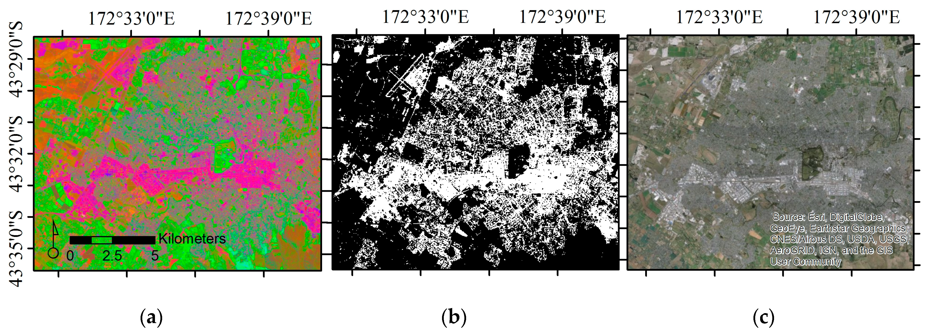
Comparison of (a) constructed RGB (R: UI, G: NDVI, B: MNDWI) (2017); (b) Binary Image (0: non-urban, 1: built-up) (2017); and (c) Aerial Image for case of Christchurch, New Zealand (Esri, DigitalGlobe 2020).
Figure 4.
Comparison of (a) constructed RGB (R: UI, G: NDVI, B: MNDWI) (2017); (b) Binary Image (0: non-urban, 1: built-up) (2017); and (c) Aerial Image for case of Christchurch, New Zealand (Esri, DigitalGlobe 2020).

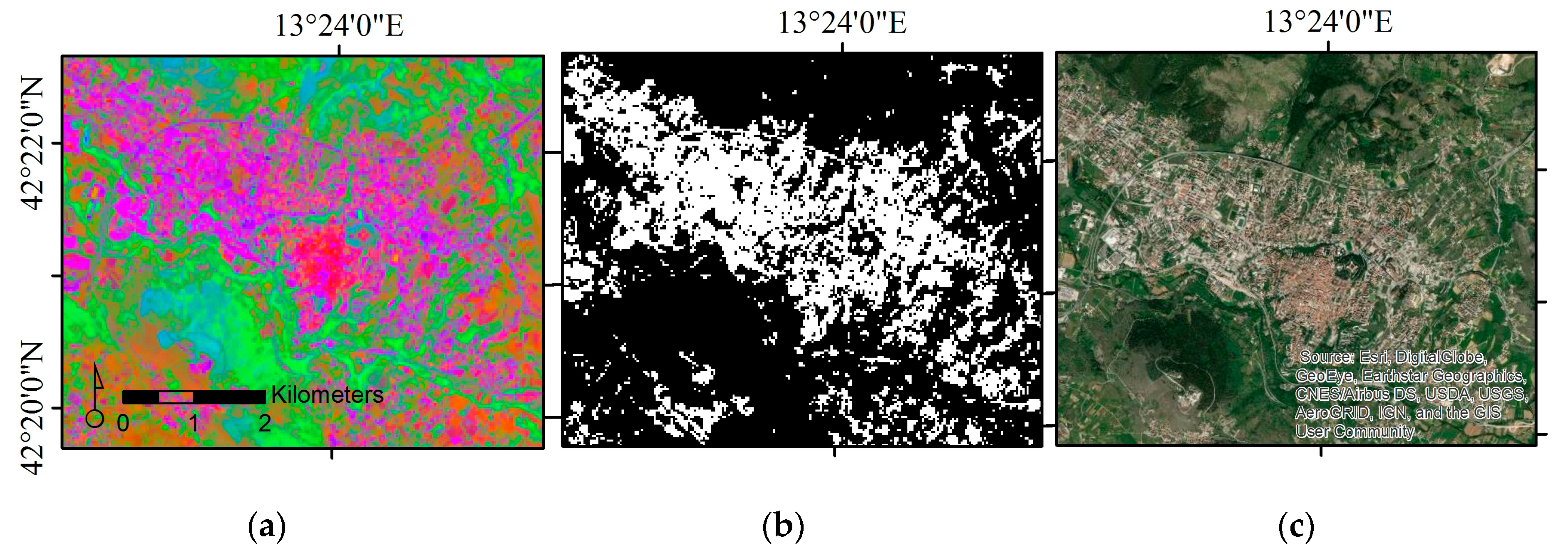
Figure 5.
Comparison of (a) constructed RGB (R: UI, G: NDVI, B: MNDWI) (2017), (b) binary image (0: non-urban, 1: built-up) (2017), and (c) aerial image for case of L’Aquila, Italy (Esri, DigitalGlobe 2020).
Figure 5.
Comparison of (a) constructed RGB (R: UI, G: NDVI, B: MNDWI) (2017), (b) binary image (0: non-urban, 1: built-up) (2017), and (c) aerial image for case of L’Aquila, Italy (Esri, DigitalGlobe 2020).

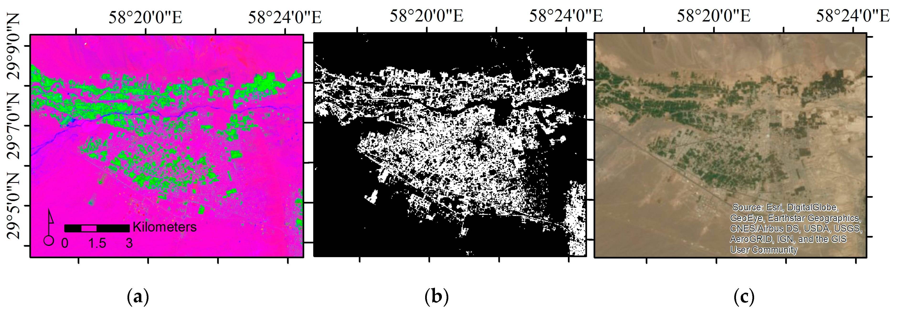
Figure 6.
Comparison of (a) constructed RGB (R: UI, G: NDVI, B: MNDWI) (2018); (b) Binary Image (0: non-urban, 1: built-up) (2018); and (c) Aerial Image for case of Bam, Iran (Esri, DigitalGlobe 2020).
Figure 6.
Comparison of (a) constructed RGB (R: UI, G: NDVI, B: MNDWI) (2018); (b) Binary Image (0: non-urban, 1: built-up) (2018); and (c) Aerial Image for case of Bam, Iran (Esri, DigitalGlobe 2020).

Figure 7.
Urban Development for Christchurch, New Zealand for (a) pre-event years (with event year), and (b) post-event.
Figure 7.
Urban Development for Christchurch, New Zealand for (a) pre-event years (with event year), and (b) post-event.

Figure 8.
Annual % Urban Land surface change for Christchurch, New Zealand (with 7.71% error variation depicted by dashed line).
Figure 8.
Annual % Urban Land surface change for Christchurch, New Zealand (with 7.71% error variation depicted by dashed line).

Figure 9.
Urban Development for L’Aquila, Italy for (a) pre-event years (with event year), and (b) post-event.
Figure 9.
Urban Development for L’Aquila, Italy for (a) pre-event years (with event year), and (b) post-event.

Figure 10.
Annual % Urban Land surface change for L’Aquila, Italy (with 8% error variation depicted by dashed line).
Figure 10.
Annual % Urban Land surface change for L’Aquila, Italy (with 8% error variation depicted by dashed line).

Figure 11.
Urban development for Bam, Iran for (a) pre-event years (with event year), and (b) post-event.
Figure 11.
Urban development for Bam, Iran for (a) pre-event years (with event year), and (b) post-event.

Figure 12.
Annual % Urban Land surface change for Bam, Iran (with 8% error variation depicted by dashed line).
Figure 12.
Annual % Urban Land surface change for Bam, Iran (with 8% error variation depicted by dashed line).

Figure 13.
Comparative overview of annual % built-up land surface change (year of the event = 0).

Figure 14.
(a) Annual % Urban/built-up Land surface change for Christchurch, New Zealand, by Districts, (b) District boundaries in the AOI for Christchurch, New Zealand.
Figure 14.
(a) Annual % Urban/built-up Land surface change for Christchurch, New Zealand, by Districts, (b) District boundaries in the AOI for Christchurch, New Zealand.

Table 1.
Summary of earthquake events and Landsat image series used for each case study.
| Country | Event | Date and Time (UTC)* | Magnitude, Intensity* | Years of Imagery |
|---|---|---|---|---|
| New Zealand | 2010 Christchurch | 2010-09-03 16:35:47 | M7.0, IX | 2000–2019 |
| Italy | 2009 L’Aquila | 2009-04-06 01:32:39 | M6.3, VIII | 1999–2019 |
| Iran | 2003 Bam | 2003-12-26 01:56:52 | M6.6, IX | 1993–2019 |
* USGS, Earthquake Hazards Program, event page.
Table 2.
Information for all Landsat image series collected for each case study.
| Information for Landsat Scenes—New Zealand (Path 74, Row 90, Spatial Resolution 30 m) | |||||
| Year | Acquisition Date | Sensor | Year | Acquisition Date | Sensor |
| 2000 | 08-MAY-00 | 7 ETM+ | 2011-Aftershock | 28-MAR-11 | 4-5 TM |
| 2001 | 02-OCT-01 | 7 ETM+ | 2011 | 30-OCT-11 | 7 ETM+ |
| 2002 | 21-OCT-02 | 7 ETM+ | 01-DEC-11 | 7 ETM+ | |
| 2003 | 16-OCT-03 | 4-5 TM | 2012 | 29-AUG-12 | 7 ETM+ |
| 2004 | 02-OCT-04 | 4-5 TM | 03-DEC-12 | 7 ETM+ | |
| 2005 | 05-OCT-05 | 4-5 TM | 2013 | 30-DEC-13 | 8 OLI |
| 2006 | 08-OCT-06 | 4-5 TM | 2014 | 28-SEP-14 | 8 OLI |
| 2007 | 16-FEB-08 | 4-5 TM | 2015 | 17-OCT-15 | 8 OLI |
| 2008 | 14-NOV-08 | 4-5 TM | 2016 | 20-NOV-16 | 8 OLI |
| 2009 | 21-FEB-10 | 4-5 TM | 2017 | 03-AUG-17 | 8 OLI |
| 2010- Earthquake | 22-DEC-10 | 4-5 TM | 2018−2019 | 02-MAR-19 | 8 OLI |
| Information for Landsat Scenes—Italy (Path 190, Row 31, Spatial Resolution 30 m) | |||||
| Year | Acquisition Date | Sensor | Year | Acquisition Date | Sensor |
| 1999 | 15-AUG-99 | 4-5 TM | 2010 | 12-JUL-10 | 4-5 TM |
| 2000 | 01-AUG-00 | 4-5 TM | 2011 | 29-JUN-11 | 4-5 TM |
| 2001 | 03-JUL-01 | 4-5 TM | 2012 | 04-APR-12 | 7 ETM+ |
| 2002 | 16-SEP-02 | 7 ETM+ | 07-JUN-12 | 7 ETM+ | |
| 2003 | 23-JUN-03 | 4-5 TM | 2013 | 05-AUG-13 | 8 OLI |
| 2004 | 09-JUN-04 | 4-5 TM | 2014 | 08-AUG-14 | 8 OLI |
| 2005 | 30-JUL-05 | 4-5 TM | 2015 | 27-AUG-15 | 8 OLI |
| 2006 | 17-JUL-06 | 4-5 TM | 2016 | 29-AUG-16 | 8 OLI |
| 2007 | 18-JUN-07 | 4-5 TM | 2017 | 31-JUL-17 | 8 OLI |
| 2008 | 03-MAY-08 | 4-5 TM | 2018 | 02-JUL-18 | 8 OLI |
| 2009-Earthquake | 25-JUL-09 | 4-5 TM | |||
| Information for Landsat Scenes—Iran (Path 159, Row 40, Spatial Resolution 30 m) | |||||
| Year | Acquisition Date | Sensor | Year | Acquisition Date | Sensor |
| 1993-94 | 27-DEC-93 | 4-5 TM | 2006-07 | 08-JAN-07 | 7 ETM+ |
| 1994-95 | 15-JAN-95 | 4-5 TM | 25-FEB-07 | 7 ETM+ | |
| 1995-96 | 01-DEC-95 | 4-5 TM | 2007-08 | 24-APR-08 | 4-5 TM |
| 1996-97 | 04-JAN-97 | 4-5 TM | 2008-09 | 05-JAN-09 | 4-5 TM |
| 1997-98 | 23-JAN-98 | 4-5 TM | 2009-10 | 24-JAN-10 | 4-5 TM |
| 1998-99 | 25-DEC-98 | 4-5 TM | 2010-11 | 26-DEC-10 | 4-5 TM |
| 1999-2000 | 28-DEC-99 | 4-5 TM | 2011-12 | 06-JAN-12 | 7 ETM+ |
| 2000-01 | 30-DEC-00 | 4-5 TM | 07-FEB-12 | 7 ETM+ | |
| 2001-02 | 18-JAN-02 | 4-5 TM | 2012-13 | 24-MAY-13 | 8 OLI |
| 2002-03 | 26-NOV-02 | 7 ETM+ | 2013-14 | 03-JAN-14 | 8 OLI |
| 2003-04-Earthquake | 16-JAN-04 | 7 ETM+ | 2014-15 | 06-JAN-15 | 8 OLI |
| 17-FEB-04 | 7 ETM+ | 2015-16 | 26-FEB-16 | 8 OLI | |
| 2004-05 | 02-JAN-05 | 7 ETM+ | 2016-17 | 28-FEB-17 | 8 OLI |
| 03-FEB-05 | 7 ETM+ | 2017-18 | 29-DEC-17 | 8 OLI | |
| 2005-06 | 05-JAN-06 | 7 ETM+ | 2018-19 | 01-JAN-19 | 8 OLI |
| 26-MAR-06 | 7 ETM+ | ||||
Table 3.
Conditional statement thresholds for each case study.
| Conditional statement thresholds for Christchurch, New Zealand | ||||||
| Year | UI | NDVI | MNDWI | |||
| Upper threshold | Lower threshold | Upper threshold | Lower threshold | Upper threshold | Lower threshold | |
| 2000 | - | −0.4214 | - | 0.3764 | 0 | −0.4559 |
| 2001 | - | −0.4481 | - | 0.3583 | 0 | −0.4370 |
| 2002 | - | −0.4366 | - | 0.3386 | 0 | −0.4425 |
| 2003 | - | −0.4429 | - | 0.3378 | 0 | −0.4340 |
| 2004 | - | −0.4323 | - | 0.3441 | 0 | −0.4609 |
| 2005 | - | −0.4086 | - | 0.3294 | 0 | −0.4589 |
| 2006 | - | −0.4123 | - | 0.3147 | 0 | −0.4588 |
| 2007 | - | −0.3685 | - | 0.2910 | 0 | −0.4529 |
| 2008 | - | −0.4260 | - | 0.3075 | 0 | −0.4112 |
| 2009 | - | −0.3895 | - | 0.3227 | 0 | −0.4204 |
| 2010 | - | −0.3702 | - | 0.2972 | 0 | −0.4552 |
| 2011 | - | −0.4013 | - | 0.3360 | 0 | −0.4480 |
| 2013 | - | −0.3841 | - | 0.2841 | 0 | −0.4425 |
| 2014 | - | −0.4214 | - | 0.3300 | 0 | −0.4403 |
| 2015 | - | −0.4206 | - | 0.3150 | 0 | −0.4431 |
| 2016 | - | −0.4121 | - | 0.3177 | 0 | −0.4433 |
| 2017 | - | −0.4167 | - | 0.3781 | 0 | −0.4562 |
| 2018 | - | −0.3907 | - | 0.3282 | 0 | −0.4402 |
| Conditional statement thresholds for L’Aquila, Italy | ||||||
| Year | UI | NDVI | MNDWI | |||
| Upper threshold | Lower threshold | Upper threshold | Lower threshold | Upper threshold | Lower threshold | |
| 1999 | - | −0.5381 | - | 0.4515 | 0 | −0.3793 |
| 2000 | - | −0.5426 | - | 0.4539 | 0 | −0.3776 |
| 2001 | - | −0.5411 | - | 0.4440 | 0 | −0.3796 |
| 2002 | - | −0.5452 | - | 0.5054 | 0 | −0.3868 |
| 2003 | - | −0.5319 | - | 0.4332 | 0 | −0.3789 |
| 2004 | - | −0.5654 | - | 0.4792 | 0 | −0.3836 |
| 2005 | - | −0.5495 | - | 0.4600 | 0 | −0.3711 |
| 2006 | - | −0.5404 | - | 0.4473 | 0 | −0.3782 |
| 2007 | - | −0.5396 | - | 0.4450 | 0 | −0.3794 |
| 2008 | - | −0.5640 | - | 0.5185 | 0 | −0.3893 |
| 2009 | - | −0.5357 | - | 0.4466 | 0 | −0.3787 |
| 2010 | - | −0.5397 | - | 0.4399 | 0 | −0.3798 |
| 2011 | - | −0.5396 | - | 0.4677 | 0 | −0.3863 |
| 2013 | - | −0.5394 | - | 0.4439 | 0 | −0.3805 |
| 2014 | - | −0.5428 | - | 0.4479 | 0 | −0.3814 |
| 2016 | - | −0.5361 | - | 0.4537 | 0 | −0.3798 |
| 2017 | - | −0.5459 | - | 0.4555 | 0 | −0.3751 |
| 2018 | - | −0.5384 | - | 0.4357 | 0 | −0.3791 |
| Conditional statement thresholds for Bam, Iran | ||||||
| Year | UI | NDVI | MNDWI | |||
| Upper threshold | Lower threshold | Upper threshold | Lower threshold | Upper threshold | Lower threshold | |
| 1994 | 0.1342 | −0.3262 | 0.3841 | 0.0777 | - | −0.1813 |
| 1995 | 0.1275 | −0.3219 | 0.3786 | 0.0798 | - | −0.1233 |
| 1996 | 0.1187 | −0.2510 | 0.2701 | 0.0459 | - | −0.1062 |
| 1997 | 0.2196 | −0.4221 | 0.4572 | 0.0675 | - | −0.1082 |
| 1998 | 0.2181 | −0.4252 | 0.4646 | 0.0699 | - | −0.1102 |
| 2000 | 0.0843 | −0.2515 | 0.2739 | 0.0746 | - | −0.1294 |
| 2001 | 0.1171 | −0.3153 | 0.3631 | 0.0852 | - | −0.1274 |
| 2002 | 0.1224 | −0.3206 | 0.3651 | 0.0872 | - | −0.1317 |
| 2003 | 0.1535 | −0.3574 | 0.4195 | 0.0854 | - | −0.1284 |
| 2008 | 0.2235 | −0.4039 | 0.4777 | 0.0819 | - | −0.1071 |
| 2009 | 0.2192 | −0.4204 | 0.4543 | 0.0705 | - | −0.1154 |
| 2010 | 0.2056 | −0.4066 | 0.4632 | 0.0726 | - | −0.1180 |
| 2011 | 0.2078 | −0.4247 | 0.4593 | 0.0738 | - | −0.1146 |
| 2013 | 0.2297 | −0.4059 | 0.4862 | 0.0799 | - | −0.1115 |
| 2014 | 0.1923 | −0.3932 | 0.4472 | 0.0745 | - | −0.1214 |
| 2015 | 0.2358 | −0.4595 | 0.5166 | 0.0812 | - | −0.1177 |
| 2016 | 0.2652 | −0.4769 | 0.5434 | 0.0735 | - | −0.1106 |
| 2017 | 0.2769 | −0.4983 | 0.5529 | 0.0756 | - | −0.1118 |
| 2018 | 0.2212 | −0.4278 | 0.4874 | 0.0755 | - | −0.1219 |
| 2019 | 0.2600 | −0.4844 | 0.5367 | 0.0770 | - | −0.1171 |
Table 4.
Accuracy assessment results.
| Accuracy Assessment | ||||
|---|---|---|---|---|
| Year | Overall Accuracy (%) | Kappa Coefficient | Producer Accuracy (%) Errors of Omission | User Accuracy (%) Errors of Commission |
| New Zealand | ||||
| 2003 | 94.29% | 0.8584 | 94.62% | 85.44% |
| 2011 | 94.29% | 0.8548 | 95.45% | 84.00% |
| 2017 | 92.29% | 0.8037 | 95.24% | 77.67% |
| Italy | ||||
| 2003 | 93.14% | 0.8302 | 93.48% | 82.69% |
| 2010 | 95.43% | 0.8846 | 97.75% | 86.14% |
| 2017 | 92.00% | 0.7987 | 96.43% | 76.42% |
| Iran | ||||
| 2001 | 92.00% | 0.8109 | 92.93% | 81.42% |
| 2009 | 93.71% | 0.8707 | 97.10% | 88.16% |
| 2018 | 96.29% | 0.9193 | 98.35% | 91.54% |
Table 5.
Summary overview of built-up area change results (for AOI).
| Case | Total AOI Area (Km2) | Pre-event | Year of Earthquake | Post-event (Current) | |||
|---|---|---|---|---|---|---|---|
| Built-Up Area Estimate (Km2) | % Change from Pre-event | Built-Up Area Estimate (Km2) | % Change from Pre-event | Built-Up Area Estimate (Km2) | % Change from Pre-event | ||
| New Zealand | 6,280.31 | 184.98 | 0.00% | 125.23 | −32.30% | 261.34 | +41.27% |
| Italy | 1,114.98 | 77.63 | 0.00% | 65.09 | −16.15% | 87.16 | +12.27% |
| Iran | 3,445.69 | 133.14 | 0.00% | 49.29 | −62.98% | 66.95 | −49.71% |
© 2020 by the authors. Licensee MDPI, Basel, Switzerland. This article is an open access article distributed under the terms and conditions of the Creative Commons Attribution (CC BY) license (http://creativecommons.org/licenses/by/4.0/).
Share and Cite
MDPI and ACS Style
Derakhshan, S.; Cutter, S.L.; Wang, C. Remote Sensing Derived Indices for Tracking Urban Land Surface Change in Case of Earthquake Recovery. Remote Sens. 2020, 12, 895. https://0-doi-org.brum.beds.ac.uk/10.3390/rs12050895
AMA Style
Derakhshan S, Cutter SL, Wang C. Remote Sensing Derived Indices for Tracking Urban Land Surface Change in Case of Earthquake Recovery. Remote Sensing. 2020; 12(5):895. https://0-doi-org.brum.beds.ac.uk/10.3390/rs12050895
Chicago/Turabian StyleDerakhshan, Sahar, Susan L. Cutter, and Cuizhen Wang. 2020. "Remote Sensing Derived Indices for Tracking Urban Land Surface Change in Case of Earthquake Recovery" Remote Sensing 12, no. 5: 895. https://0-doi-org.brum.beds.ac.uk/10.3390/rs12050895
Note that from the first issue of 2016, this journal uses article numbers instead of page numbers. See further details here.