Current Practices in UAS-based Environmental Monitoring

 ,
,  , , ,
, , ,  ,
,  ,
,  , ,
, ,  , , ,
, , ,  , ,
, , 
Abstract
:
1. Introduction
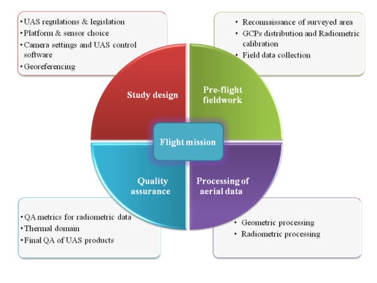
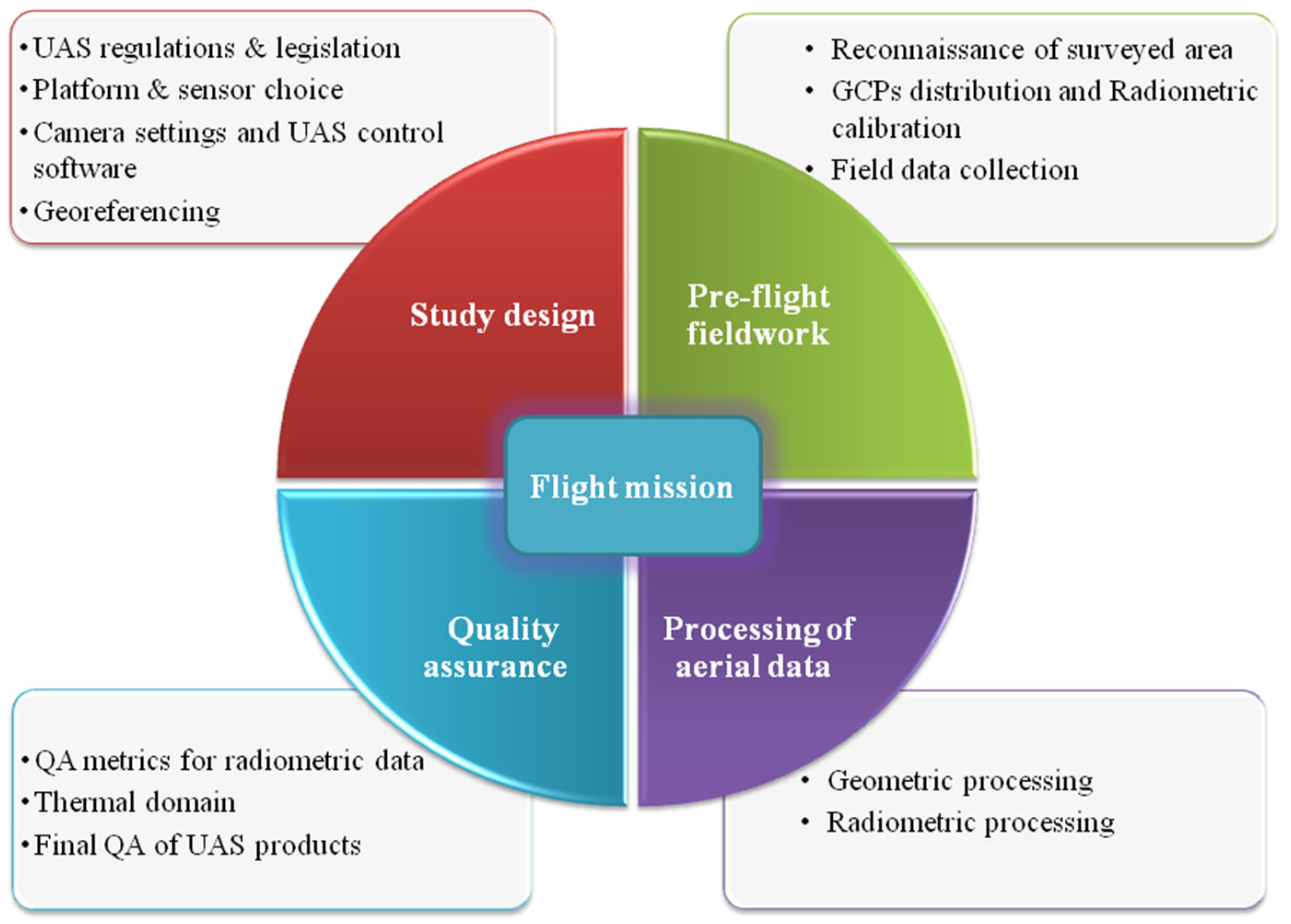
2. Study Design
2.1. UAS Regulations and Legislation
2.2. Platform and Sensor Choice
2.3. Camera Settings and UAS Control Software
2.4. Georeferencing
- errors generated from external orientation sensors (e.g., GNSS and internal measurement unit—IMU errors);
- errors generated from internal orientation procedure (e.g., stability of the focal length, lens distortion, over-parameterization through self-calibration);
- errors generated from the measurement of image point coordinates.
3. Pre-Flight Fieldwork
3.1. Reconnaissance of the Surveyed Area
3.2. Ground Control Point Distribution and Radiometric Calibration
3.3. Field Data Collection
4. Flight Mission
5. Processing of Aerial Data
5.1. Geometric Processing
5.2. Radiometric Processing
6. Quality Assurance
6.1. Quality Assurance Metrics for Radiometric Data
6.2. Thermal Domain
6.3. Final Quality Assurance of UAS Products
7. Discussion and Final Remarks
8. Conclusions
Author Contributions
Funding
Conflicts of Interest
Appendix A. Checklists Before A Flight

| N. | HARMONIOUS UAS Check-List | Check |
|---|---|---|
| 1 | Check the weather conditions (particularly critical maybe rain and strong wind) | |
| 2 | Identify the timing of the flight with respect to the best solar illumination. The central hours of the day allow avoiding shadows in the scene. | |
| 3 | Make sure that you have GPS coverage to fly in “safe” mode. | |
| 4 | Take off from areas that are sufficiently large, free of obstacles and leveled | |
| 5 | Check the presence of any deformation to the propeller or frames | |
| 6 | Execute a small manual flight; this ensures that the vehicle is stable and radio control is performing well | |
| 7 | If the presence of people and / or animals is planned in the survey area, plan the flight when such presence is minimum. | |
| 8 | In the case of critical operations, obtain all permits in advance | |
| 9 | Check the status of the batteries of your drone, controller, sensors, and tablet | |
| 10 | Check that the propellers are intact and well-fixed | |
| 11 | Deactivate for safety the Bluetooth and the Wi-Fi of your device (we recommend the mode “Airplane”) | |
| 12 | Check that you have enough free memory in the SD card used to store the data acquired | |
| 13 | Do the compass calibration (magnetic compass) | |
| 14 | Wait for the drone to connect to as many satellites as possible (minimum required 5) | |
| 15 | Set the “return to home” point in case of anomaly before starting | |
| 16 | Take off and Fly |
Appendix B. UAS-Survey Description
| Study design | Platform characteristics | Platform type |
| Weight & payload capacity | ||
| Maximum speed | ||
| Flight height & coverage | ||
| On-board GNSS receiver | ||
| Sensor characteristics | Sensor type & name | |
| Sensor weight | ||
| Camera settings | Pixel size | |
| Sensor size | ||
| Focal length | ||
| ISO | ||
| Aperture | ||
| Shutter Speed | ||
| Flight plan | GSD (cm) | |
| Flight height | ||
| Flight speed | ||
| Forward & side image overlap | ||
| UAS Control software | Software name | |
| Georeferencing | Type of georeferencing | |
| Number of GCPs | ||
| Arrangement of GCPs | ||
| Flight mission | Weather | Wind power & direction |
| Illumination condition | ||
| Humidity | ||
| Mission | Average flying speed | |
| Flying time | ||
| Flight pattern | ||
| Camera angle | ||
| Image format | ||
| Processing of aerial data | Geometric processing | SfM tool name |
| Final product type | ||
| Bundle adjustment | ||
| Radiometric processing | Signal to noise ratio | |
| Radiometric resolution | ||
| Viewing geometry | ||
| Band configuration | ||
| Reflectance calculation method | ||
| Vignetting | ||
| Motion blur | ||
| Accuracy assessment | Error measure | |
| Statistical value | ||
| Error management | ||
| Classification accuracy |
References
- Adão, T.; Hruška, J.; Pádua, L.; Bessa, J.; Peres, E.; Morais, R.; Sousa, J.J. Hyperspectral Imaging: A Review on UAV-Based Sensors, Data Processing and Applications for Agriculture and Forestry. Remote Sens. 2017, 9, 1110. [Google Scholar] [CrossRef] [Green Version]
- Dandois, J.; Olano, M.; Ellis, E. Optimal Altitude, Overlap, and Weather Conditions for Computer Vision UAV Estimates of Forest Structure. Remote Sens. 2015, 7, 13895–13920. [Google Scholar] [CrossRef] [Green Version]
- Lisein, J.; Pierrot-Deseilligny, M.; Bonnet, S.; Lejeune, P. A Photogrammetric Workflow for the Creation of a Forest Canopy Height Model from Small Unmanned Aerial System Imagery. Forests 2013, 4, 922–944. [Google Scholar] [CrossRef] [Green Version]
- Alvarez-Taboada, F.; Paredes, C.; Julián-Pelaz, J. Mapping of the Invasive Species Hakea sericea Using Unmanned Aerial Vehicle (UAV) and WorldView-2 Imagery and an Object-Oriented Approach. Remote Sens. 2017, 9, 913. [Google Scholar] [CrossRef] [Green Version]
- Mesas-Carrascosa, F.J.; Clavero Rumbao, I.; Torres-Sánchez, J.; García-Ferrer, A.; Peña, J.M.; López Granados, F. Accurate ortho-mosaicked six-band multispectral UAV images as affected by mission planning for precision agriculture proposes. Int. J. Remote Sens. 2017, 38, 2161–2176. [Google Scholar] [CrossRef]
- Yuan, W.; Li, J.; Bhatta, M.; Shi, Y.; Baenziger, P.; Ge, Y. Wheat Height Estimation Using LiDAR in Comparison to Ultrasonic Sensor and UAS. Sensors 2018, 18, 3731. [Google Scholar] [CrossRef] [Green Version]
- Tauro, F.; Pagano, C.; Phamduy, P.; Grimaldi, S.; Porfiri, M. Large-Scale Particle Image Velocimetry from an Unmanned Aerial Vehicle. IEEE ASME Trans. Mechatron. 2015, 20, 3269–3275. [Google Scholar] [CrossRef]
- James, M.R.; Robson, S.; d’Oleire-Oltmanns, S.; Niethammer, U. Optimising UAV topographic surveys processed with structure-from-motion: Ground control quality, quantity and bundle adjustment. Geomorphology 2017, 280, 51–66. [Google Scholar] [CrossRef] [Green Version]
- Whitehead, K.; Hugenholtz, C.H. Applying ASPRS Accuracy Standards to Surveys from Small Unmanned Aircraft Systems (UAS). Photogramm. Eng. Remote Sens. 2015, 81, 787–793. [Google Scholar] [CrossRef]
- Gomez, C.; Purdie, H. UAV-based Photogrammetry and Geocomputing for Hazards and Disaster Risk Monitoring—A Review. Geoenviron. Disasters 2016, 3, 23. [Google Scholar] [CrossRef] [Green Version]
- Manfreda, S.; McCabe, M.; Miller, P.; Lucas, R.; Pajuelo Madrigal, V.; Mallinis, G.; Ben Dor, E.; Helman, D.; Estes, L.; Ciraolo, G.; et al. On the Use of Unmanned Aerial Systems for Environmental Monitoring. Remote Sens. 2018, 10, 641. [Google Scholar] [CrossRef] [Green Version]
- Ewertowski, M.W.; Tomczyk, A.M.; Evans, D.J.A.; Roberts, D.H.; Ewertowski, W. Operational Framework for Rapid, Very-high Resolution Mapping of Glacial Geomorphology Using Low-cost Unmanned Aerial Vehicles and Structure-from-Motion Approach. Remote Sens. 2019, 11, 65. [Google Scholar] [CrossRef] [Green Version]
- Rusnák, M.; Sládek, J.; Kidová, A.; Lehotský, M. Template for high-resolution river landscape mapping using UAV technology. Measurement 2018, 115, 139–151. [Google Scholar] [CrossRef]
- Hamada, Y.; Stow, D.A.; Coulter, L.L.; Jafolla, J.C.; Hendricks, L.W. Detecting Tamarisk species (Tamarix spp.) in riparian habitats of Southern California using high spatial resolution hyperspectral imagery. Remote Sens. Environ. 2007, 109, 237–248. [Google Scholar] [CrossRef]
- Pande-Chhetri, R.; Abd-Elrahman, A.; Liu, T.; Morton, J.; Wilhelm, V.L. Object-based classification of wetland vegetation using very high-resolution unmanned air system imagery. Eur. J. Remote Sens. 2017, 50, 564–576. [Google Scholar] [CrossRef] [Green Version]
- Assmann, J.J.; Kerby, J.T.; Cunliffe, A.M.; Myers-Smith, I.H. Vegetation monitoring using multispectral sensors—Best practices and lessons learned from high latitudes. J. Unmanned Veh. Syst. 2019, 7, 54–75. [Google Scholar] [CrossRef] [Green Version]
- Aasen, H.; Honkavaara, E.; Lucieer, A.; Zarco-Tejada, P. Quantitative Remote Sensing at Ultra-High Resolution with UAV Spectroscopy: A Review of Sensor Technology, Measurement Procedures, and Data Correction Workflows. Remote Sens. 2018, 10, 1091. [Google Scholar] [CrossRef] [Green Version]
- Gini, R.; Passoni, D.; Pinto, L.; Sona, G. Use of Unmanned Aerial Systems for multispectral survey and tree classification: A test in a park area of northern Italy. Eur. J. Remote Sens. 2014, 47, 251–269. [Google Scholar] [CrossRef]
- Ma, L.; Li, M.; Ma, X.; Cheng, L.; Du, P.; Liu, Y. A review of supervised object-based land-cover image classification. ISPRS J. Photogramm. Remote Sens. 2017, 130, 277–293. [Google Scholar] [CrossRef]
- Singh, K.K.; Frazier, A.E. A meta-analysis and review of unmanned aircraft system (UAS) imagery for terrestrial applications. Int. J. Remote Sens. 2018, 39, 5078–5098. [Google Scholar] [CrossRef]
- Barreto, M.A.P.; Johansen, K.; Angel, Y.; McCabe, M.F. Radiometric Assessment of a UAV-Based Push-Broom Hyperspectral Camera. Sensors 2019, 19, 4699. [Google Scholar] [CrossRef] [PubMed] [Green Version]
- Müllerová, J.; Brůna, J.; Bartaloš, T.; Dvořák, P.; Vítková, M.; Pyšek, P. Timing Is Important: Unmanned Aircraft vs. Satellite Imagery in Plant Invasion Monitoring. Front. Plant Sci. 2017, 8, 887. [Google Scholar] [CrossRef] [PubMed] [Green Version]
- Whitehead, K.; Hugenholtz, C.H. Remote sensing of the environment with small unmanned aircraft systems (UASs), part 1: A review of progress and challenges. J. Unmanned Veh. Syst. 2014, 2, 69–85. [Google Scholar] [CrossRef]
- Morgenthal, G.; Hallermann, N. Quality assessment of unmanned aerial vehicle (UAV) based visual inspection of structures. Adv. Struct. Eng. 2014, 17, 289–302. [Google Scholar] [CrossRef]
- Tziavou, O.; Pytharouli, S.; Souter, J. Unmanned Aerial Vehicle (UAV) based mapping in engineering geological surveys: Considerations for optimum results. Eng. Geol. 2018, 232, 12–21. [Google Scholar] [CrossRef] [Green Version]
- Ahmadzadeh, A.; Jadbabaie, A.; Kumar, V.; Pappas, G.J. Multi-UAV cooperative surveillance with spatio-temporal specifications. In Proceedings of the 45th IEEE Conference on Decision and Control, San Diego, CA, USA, 13–15 December 2006; pp. 5293–5298. [Google Scholar]
- Kontogiannis, S.G.; Ekaterinaris, J.A. Design, performance evaluation and optimization of a UAV. Aerosp. Sci. Technol. 2013, 29, 339–350. [Google Scholar] [CrossRef]
- Kedzierski, M.; Wierzbicki, D. Radiometric quality assessment of images acquired by UAV’s in various lighting and weather conditions. Measurement 2015, 76, 156–169. [Google Scholar] [CrossRef]
- Chen, H.; Wang, X.M.; Jiao, Y.S.; Li, Y. Research on search probability and camera footprint of region coverage for UAVs. In Proceedings of the IEEE International Conference on Control and Automation, Christchurch, New Zealand, 9–11 December 2009; pp. 1920–1924. [Google Scholar]
- Cruzan, M.B.; Weinstein, B.G.; Grasty, M.R.; Kohrn, B.F.; Hendrickson, E.C.; Arredondo, T.M.; Thompson, P.G. Small unmanned aerial vehicles (micro-UAVs, drones) in plant ecology. Appl. Plant Sci. 2016, 4, 1600041. [Google Scholar] [CrossRef]
- Stöcker, C.; Bennett, R.; Nex, F.; Gerke, M.; Zevenbergen, J. Review of the Current State of UAV Regulations. Remote Sens. 2017, 9, 459. [Google Scholar] [CrossRef] [Green Version]
- EU Commission Delegated Regulation (EU) 2019/945 on unmanned aircraft systems and on third-country operators of unmanned aircraft systems. Off. Journey 2019, L152, 1–40.
- Shi, Y.; Thomasson, J.A.; Murray, S.C.; Pugh, N.A.; Rooney, W.L.; Shafian, S.; Rajan, N.; Rouze, G.; Morgan, C.L.S.; Neely, H.L.; et al. Unmanned Aerial Vehicles for High-Throughput Phenotyping and Agronomic Research. PLoS ONE 2016, 11, e0159781. [Google Scholar] [CrossRef] [PubMed] [Green Version]
- Michez, A.; Piégay, H.; Lisein, J.; Claessens, H.; Lejeune, P. Classification of riparian forest species and health condition using multi-temporal and hyperspatial imagery from unmanned aerial system. Environ. Monit. Assess. 2016, 188, 146. [Google Scholar] [CrossRef] [PubMed] [Green Version]
- Müllerová, J.; Brůna, J.; Dvořák, P.; Bartaloš, T.; Vítková, M. Does the Data Resolution/Origin Matter? Satellite, Airborne and UAV Imagery and UAV Imagery to Tackle Plant Invasions. Int. Arch. Photogramm. Remote Sens. Spat. Inf. Sci. 2016, 41, 903–908. [Google Scholar] [CrossRef]
- Gini, R.; Sona, G.; Ronchetti, G.; Passoni, D.; Pinto, L. Improving Tree Species Classification Using UAS Multispectral Images and Texture Measures. ISPRS Int. J. Geo-Inf. 2018, 7, 315. [Google Scholar] [CrossRef] [Green Version]
- Lu, B.; He, Y. Species classification using Unmanned Aerial Vehicle (UAV)-acquired high spatial resolution imagery in a heterogeneous grassland. ISPRS J. Photogramm. Remote Sens. 2017, 128, 73–85. [Google Scholar] [CrossRef]
- Wan, L.; Li, Y.; Cen, H.; Zhu, J.; Yin, W.; Wu, W.; Zhu, H.; Sun, D.; Zhou, W.; He, Y. Combining UAV-Based Vegetation Indices and Image Classification to Estimate Flower Number in Oilseed Rape. Remote Sens. 2018, 10, 1484. [Google Scholar] [CrossRef] [Green Version]
- Weil, G.; Lensky, I.; Resheff, Y.; Levin, N. Optimizing the Timing of Unmanned Aerial Vehicle Image Acquisition for Applied Mapping of Woody Vegetation Species Using Feature Selection. Remote Sens. 2017, 9, 1130. [Google Scholar] [CrossRef] [Green Version]
- Komárek, J.; Klouček, T.; Prošek, J. The potential of Unmanned Aerial Systems: A tool towards precision classification of hard-to-distinguish vegetation types? Int. J. Appl. Earth Obs. Geoinf. 2018, 71, 9–19. [Google Scholar] [CrossRef]
- Yang, G.; Liu, J.; Zhao, C.; Li, Z.; Huang, Y.; Yu, H.; Xu, B.; Yang, X.; Zhu, D.; Zhang, X.; et al. Unmanned Aerial Vehicle Remote Sensing for Field-Based Crop Phenotyping: Current Status and Perspectives. Front. Plant Sci. 2017, 8, 1111. [Google Scholar] [CrossRef]
- Perich, G.; Hund, A.; Anderegg, J.; Roth, L.; Boer, M.P.; Walter, A.; Liebisch, F.; Aasen, H. Assessment of Multi-Image Unmanned Aerial Vehicle Based High-Throughput Field Phenotyping of Canopy Temperature. Front. Plant Sci. 2020, 11, 150. [Google Scholar] [CrossRef]
- Soto-Estrada, E.; Correa-Echeveri, S.; Posada-Posada, M. Thermal analysis of urban land cover using an unmaned aerial vehicle (UAV) in Medellin, Colombia. J. Urban Environ. Eng. 2017, 11, 142–149. [Google Scholar] [CrossRef]
- Anweiler, S.; Piwowarski, D.; Ulbrich, R. Unmanned Aerial Vehicles for Environmental Monitoring with Special Reference to Heat Loss. E3S Web Conf. 2017, 19, 02005. [Google Scholar] [CrossRef] [Green Version]
- Spaan, D.; Burke, C.; McAree, O.; Aureli, F.; Rangel-Rivera, C.E.; Hutschenreiter, A.; Longmore, S.N.; McWhirter, P.R.; Wich, S.A. Thermal Infrared Imaging from Drones Offers a Major Advance for Spider Monkey Surveys. Drones 2019, 3, 34. [Google Scholar] [CrossRef] [Green Version]
- Dinuls, R.; Erins, G.; Lorencs, A.; Mednieks, I.; Sinica-Sinavskis, J. Tree Species Identification in Mixed Baltic Forest Using LiDAR and Multispectral Data. J. Sel. Top. Appl. Earth Obs. Remote Sens. 2012, 5, 594–603. [Google Scholar] [CrossRef]
- Sankey, T.; Donager, J.; McVay, J.; Sankey, J.B. UAV lidar and hyperspectral fusion for forest monitoring in the southwestern USA. Remote Sens. Environ. 2017, 195, 30–43. [Google Scholar] [CrossRef]
- O’Connor, J.; Smith, M.J.; James, M.R. Cameras and settings for aerial surveys in the geosciences. Prog. Phys. Geogr. 2017, 41, 325–344. [Google Scholar] [CrossRef] [Green Version]
- Mosbrucker, A.R.; Major, J.J.; Spicer, K.R.; Pitlick, J. Camera system considerations for geomorphic applications of SfM photogrammetry. Earth Surf. Proc. Landf. 2017, 42, 969–986. [Google Scholar] [CrossRef] [Green Version]
- Roth, L.; Hund, A.; Aasen, H. PhenoFly Planning Tool: Flight planning for high-resolution optical remote sensing with unmanned aerial systems. Plant Methods 2018, 14, 116. [Google Scholar] [CrossRef] [Green Version]
- Boesch, R. Thermal remote sensing with UAV-based workflows. Int. Arch. Photogramm. Remote Sens. Spat. Inf. Sci. 2017, 42, 41. [Google Scholar] [CrossRef] [Green Version]
- Aasen, H.; Bolten, A. Multi-temporal high-resolution imaging spectroscopy with hyperspectral 2D imagers—From theory to application. Remote Sens. Environ. 2018, 205, 374–389. [Google Scholar] [CrossRef]
- Küng, O.; Strecha, C.; Beyeler, A.; Zufferey, J.C.; Floreano, D.; Fua, P.; Gervaix, F. The accuracy of automatic photogrammetric techniques on ultra-light UAV imagery. In Proceedings of the UAV-g 2011—Unmanned Aerial Vehicle in Geomatics, Zürich, Switzerland, 14–16 September 2011. [Google Scholar]
- Colomina, I.; Molina, P. Unmanned aerial systems for photogrammetry and remote sensing: A review. ISPRS J. Photogramm. Remote Sens. 2014, 92, 79–97. [Google Scholar] [CrossRef] [Green Version]
- Mayr, E. Storia del Pensiero Biologico. Diversità, Evoluzione, Eredità; Bollati Boringhieri: Torino, Italy, 2011; ISBN 9788833922706. [Google Scholar]
- Gonçalves, J.A.; Henriques, R. UAV photogrammetry for topographic monitoring of coastal areas. ISPRS J. Photogramm. Remote Sens. 2015, 104, 101–111. [Google Scholar] [CrossRef]
- Uysal, M.; Toprak, A.S.; Polat, N. DEM generation with UAV Photogrammetry and accuracy analysis in Sahitler hill. Measurement 2015, 73, 539–543. [Google Scholar] [CrossRef]
- Ahmed, O.S.; Shemrock, A.; Chabot, D.; Dillon, C.; Williams, G.; Wasson, R.; Franklin, S.E. Hierarchical land cover and vegetation classification using multispectral data acquired from an unmanned aerial vehicle. Int. J. Remote Sens. 2017, 38, 2037–2052. [Google Scholar] [CrossRef]
- Haala, N.; Cramer, M.; Weimer, F.; Trittler, M. Performance test on UAV-based photogrammetric data collection. Int. Arch. Photogramm. Remote Sens. Spat. Inf. Sci. 2012, 38, 7–12. [Google Scholar] [CrossRef] [Green Version]
- Seifert, E.; Seifert, S.; Vogt, H.; Drew, D.; van Aardt, J.; Kunneke, A.; Seifert, T. Influence of Drone Altitude, Image Overlap, and Optical Sensor Resolution on Multi-View Reconstruction of Forest Images. Remote Sens. 2019, 11, 1252. [Google Scholar] [CrossRef] [Green Version]
- Tu, Y.H.; Phinn, S.; Johansen, K.; Robson, A.; Wu, D. Optimising drone flight planning for measuring horticultural tree crop structure. ISPRS J. Photogramm. Remote Sens. 2020, 160, 83–96. [Google Scholar] [CrossRef] [Green Version]
- MAVProxy. Available online: https://ardupilot.github.io/MAVProxy/html/index.html (accessed on 24 February 2020).
- Mission Planner. Available online: http://ardupilot.org/planner/ (accessed on 24 February 2020).
- APM Planner 2. Available online: http://ardupilot.org/planner2/ (accessed on 24 February 2020).
- QGroundControl. Available online: http://www.qgroundcontrol.org (accessed on 24 February 2020).
- UgCS. Available online: https://www.ugcs.com (accessed on 24 February 2020).
- Ramirez-Atencia, C.; Camacho, D. Extending QGroundControl for Automated Mission Planning of UAVs. Sensors 2018, 18, 2339. [Google Scholar] [CrossRef] [Green Version]
- eMotion 3. Available online: https://www.sensefly.com/software/emotion) (accessed on 24 February 2020).
- Jacobsen, K. Exterior Orientation Parameters. Photogramm. Eng. Remote Sens. 2001, 67, 12–47. [Google Scholar]
- Kraus, K. Photogrammetry: Geometry from Images and Laser Scans; Walter de Gruyter: Berlin, Germany, 2007. [Google Scholar]
- Cramer, M.; Przybilla, H.J.; Zurhorst, A. UAV cameras: Overview and geometric calibration benchmark. Int. Arch. Photogramm. Remote Sens. Spat. Inf. Sci. 2017, 42, 85. [Google Scholar] [CrossRef] [Green Version]
- Tomaštík, J.; Mokroš, M.; Surový, P.; Grznárová, A.; Merganič, J. UAV RTK/PPK Method—An Optimal Solution for Mapping Inaccessible Forested Areas? Remote Sens. 2019, 11, 721. [Google Scholar] [CrossRef] [Green Version]
- Manfreda, S.; Dvorak, P.; Mullerova, J.; Herban, S.; Vuono, P.; Arranz Justel, J.; Perks, M. Assessing the Accuracy of Digital Surface Models Derived from Optical Imagery Acquired with Unmanned Aerial Systems. Drones 2019, 3, 15. [Google Scholar] [CrossRef] [Green Version]
- Stöcker, C.; Nex, F.; Koeva, M.; Gerke, M. Quality assessment of combined IMU/GNSS data for direct georeferencing in the context of UAV-based mapping. Int. Arch. Photogramm. Remote Sens. Spat. Inf. Sci. 2017, 42, 355. [Google Scholar] [CrossRef] [Green Version]
- Schenk, T. Towards automatic aerial triangulation. ISPRS J. Photogramm. Remote Sens. 1997, 52, 110–121. [Google Scholar] [CrossRef]
- Cramer, M.; Haala, N.; Stallmann, D. Direct Georeferencing Using GPS/Inertial Exterior Orientations for Photogrammetric Applications. ISPRS J. Photogramm. Remote Sens. 2000, 33, 198–205. [Google Scholar]
- Padró, J.-C.; Muñoz, F.-J.; Planas, J.; Pons, X. Comparison of four UAV georeferencing methods for environmental monitoring purposes focusing on the combined use with airborne and satellite remote sensing platforms. Int. J. Appl. Earth Obs. Geoinf. 2019, 75, 130–140. [Google Scholar] [CrossRef]
- Bonali, F.L.; Tibaldi, A.; Marchese, F.; Fallati, L.; Russo, E.; Corselli, C.; Savini, A. UAV-based surveying in volcano-tectonics: An example from the Iceland rift. J. Struct. Geol. 2019, 121, 46–64. [Google Scholar] [CrossRef]
- Baiocchi, V.; Napoleoni, Q.; Tesei, M.; Servodio, G.; Alicandro, M.; Costantino, D. UAV for monitoring the settlement of a landfill. Eur. J. Remote Sens. 2019, 52, 41–52. [Google Scholar] [CrossRef]
- Chudley, T.; Christoffersen, P.; Doyle, S.H.; Abellan, A.; Snooke, N. High accuracy UAV photogrammetry of ice sheet dynamics with no ground control. Cryosphere 2019, 13, 955–968. [Google Scholar] [CrossRef] [Green Version]
- Chudley, T.R.; Christoffersen, P.; Doyle, S.H.; Bougamont, M.; Schoonman, C.M.; Hubbard, B.; James, M.R. Supraglacial lake drainage at a fast-flowing Greenlandic outlet glacier. Proc. Natl. Acad. Sci. USA 2019, 116, 25468–25477. [Google Scholar] [CrossRef]
- Zhang, H.; Aldana-Jague, E.; Clapuyt, F.; Wilken, F.; Vanacker, V.; Van Oost, K. Evaluating the potential of post-processing kinematic (PPK) georeferencing for UAV-based structure- from-motion (SfM) photogrammetry and surface change detection. Earth Surf. Dyn. 2019, 7, 807–827. [Google Scholar] [CrossRef] [Green Version]
- Grayson, B.; Penna, N.T.; Mills, J.P.; Grant, D.S. GPS precise point positioning for UAV photogrammetry. Photogramm. Rec. 2018, 33, 427–447. [Google Scholar] [CrossRef] [Green Version]
- James, M.R.; Chandler, J.H.; Eltner, A.; Fraser, C.; Miller, P.E.; Mills, J.P.; Noble, T.; Robson, S.; Lane, S.N. Guidelines on the use of structure-from-motion photogrammetry in geomorphic research. Earth Surf. Proc. Landf. 2019, 44, 2081–2084. [Google Scholar] [CrossRef]
- Höhle, J.; Höhle, M. Accuracy assessment of digital elevation models by means of robust statistical methods. ISPRS J. Photogramm. Remote Sens. 2009, 64, 398–406. [Google Scholar] [CrossRef] [Green Version]
- Gonçalves, G.R.; Pérez, J.A.; Duarte, J. Accuracy and effectiveness of low cost UASs and open source photogrammetric software for foredunes mapping. Int. J. Remote Sens. 2018, 39, 5059–5077. [Google Scholar] [CrossRef]
- Rock, G.; Ries, J.B.; Udelhoven, T. Sensitivity analysis of UAV-photogrammetry for creating Digital Elevation Models (DEM). Int. Arch. Photogramm. Remote Sens. Spat. Inf. Sci. 2012, 38, 69–73. [Google Scholar] [CrossRef] [Green Version]
- Dunford, R.; Michel, K.; Gagnage, M.; Piégay, H.; Trémelo, M.L. Potential and constraints of Unmanned Aerial Vehicle technology for the characterization of Mediterranean riparian forest. Int. J. Remote Sens. 2009, 30, 4915–4935. [Google Scholar] [CrossRef]
- Tonkin, T.; Midgley, N. Ground-Control Networks for Image Based Surface Reconstruction: An Investigation of Optimum Survey Designs Using UAV Derived Imagery and Structure-from-Motion Photogrammetry. Remote Sens. 2016, 8, 786. [Google Scholar] [CrossRef] [Green Version]
- Martínez-Carricondo, P.; Agüera-Vega, F.; Carvajal-Ramírez, F.; Mesas-Carrascosa, F.-J.; García-Ferrer, A.; Pérez-Porras, F.-J. Assessment of UAV-photogrammetric mapping accuracy based on variation of ground control points. Int. J. Appl. Earth Obs. Geoinf. 2018, 72, 1–10. [Google Scholar] [CrossRef]
- Rangel, J.M.G.; Gonçalves, G.R.; Pérez, J.A. The impact of number and spatial distribution of GCPs on the positional accuracy of geospatial products derived from low-cost UASs. Int. J. Remote Sens. 2018, 39, 7154–7171. [Google Scholar] [CrossRef]
- Oniga, V.-E.; Breaban, A.-I.; Statescu, F. Determining the Optimum Number of Ground Control Points for Obtaining High Precision Results Based on UAS Images. Proceedings 2018, 2, 352. [Google Scholar] [CrossRef] [Green Version]
- Duan, Y.; Yan, L.; Xiang, Y.; Gou, Z.; Chen, W.; Jing, X. Design and experiment of UAV remote sensing optical targets. In Proceedings of the 2011 International Conference on Electronics, Communications and Control (ICECC 2011), Ningbo, China, 9–11 September 2011; pp. 202–205. [Google Scholar]
- Grenzdörffer, G.J.; Niemeyer, F. UAV based BRDF-measurements of agricultural surfaces with pfiffikus. Int. Arch. Photogramm. Remote Sens. Spat. Inf. Sci. 2012, 38, 229–234. [Google Scholar] [CrossRef] [Green Version]
- Laliberte, A.S.; Goforth, M.A.; Steele, C.M.; Rango, A. Multispectral Remote Sensing from Unmanned Aircraft: Image Processing Workflows and Applications for Rangeland Environments. Remote Sens. 2011, 3, 2529–2551. [Google Scholar] [CrossRef] [Green Version]
- Nebiker, S.; Annen, A.; Scherrer, M.; Oesch, D. A Light-weight Multispectral Sensor for Micro UAV-Opportunities for very High Resolution Airborne Remote Sensing. Int. Arch. Photogramm. Remote Sens. Spat. Inf. Sci. 2008, 37, 1193–1200. [Google Scholar]
- Bondi, E.; Salvaggio, C.; Montanaro, M.; Gerace, A.D. Calibration of UAS imagery inside and outside of shadows for improved vegetation index computation. Auton. Air Ground Sens. Syst. Agric. Optim. Phenotyping 2016, 9866, 98660J. [Google Scholar]
- Näsi, R.; Honkavaara, E.; Lyytikäinen-Saarenmaa, P.; Blomqvist, M.; Litkey, P.; Hakala, T.; Viljanen, N.; Kantola, T.; Tanhuanpää, T.; Holopainen, M. Using UAV-Based Photogrammetry and Hyperspectral Imaging for Mapping Bark Beetle Damage at Tree-Level. Remote Sens. 2015, 7, 15467–15493. [Google Scholar] [CrossRef] [Green Version]
- Hakala, T.; Markelin, L.; Honkavaara, E.; Scott, B.; Theocharous, T.; Nevalainen, O.; Näsi, R.; Suomalainen, J.; Viljanen, N.; Greenwell, C.; et al. Direct Reflectance Measurements from Drones: Sensor Absolute Radiometric Calibration and System Tests for Forest Reflectance Characterization. Sensors 2018, 18, 1417. [Google Scholar] [CrossRef] [Green Version]
- Honkavaara, E.; Hakala, T.; Nevalainen, O.; Viljanen, N.; Rosnell, T.; Khoramshahi, E.; Näsi, R.; Oliveira, R.; Tommaselli, A. Geometric and reflectance signature characterization of complex canopies using hyperspectral stereoscopic images from UAV amd terrestrial platrforms. Int. Arch. Photogramm. Remote Sens. Spat. Inf. Sci. 2016, 41, 77–82. [Google Scholar] [CrossRef]
- Johansen, K.; Raharjo, T.; McCabe, M. Using Multi-Spectral UAV Imagery to Extract Tree Crop Structural Properties and Assess Pruning Effects. Remote Sens. 2018, 10, 854. [Google Scholar] [CrossRef] [Green Version]
- James, M.R.; Robson, S. Mitigating systematic error in topographic models derived from UAV and ground-based image networks. Earth Surf. Proc. Landf. 2014, 39, 1413–1420. [Google Scholar] [CrossRef] [Green Version]
- Bash, E.; Moorman, B.; Gunther, A. Detecting Short-Term Surface Melt on an Arctic Glacier Using UAV Surveys. Remote Sens. 2018, 10, 1547. [Google Scholar] [CrossRef] [Green Version]
- Klingbeil, L.; Heinz, E.; Wieland, M.; Eichel, J.; Laebe, T.; Kuhlmann, H. On the UAV based Analysis of Slow Geomorphological Processes: A Case Study at a Solifluction Lobe in the Turtmann Valley. In Proceedings of the 4th Joint International Symposium on Deformation Monitoring (JISDM 2019), Athens, Greece, 15–17 May 2019. [Google Scholar]
- Ge, X.; Wang, J.; Ding, J.; Cao, X.; Zhang, Z.; Liu, J.; Li, X. Combining UAV-based hyperspectral imagery and machine learning algorithms for soil moisture content monitoring. PeerJ 2019, 7, e6926. [Google Scholar] [CrossRef] [PubMed]
- Hassan-Esfahani, L.; Torres-Rua, A.; Jensen, A.; McKee, M. Assessment of Surface Soil Moisture Using High-Resolution Multi-Spectral Imagery and Artificial Neural Networks. Remote Sens. 2015, 7, 2627–2646. [Google Scholar] [CrossRef] [Green Version]
- Luo, W.; Xu, X.; Liu, W.; Liu, M.; Li, Z.; Peng, T.; Xu, C.; Zhang, Y.; Zhang, R. UAV based soil moisture remote sensing in a karst mountainous catchment. Catena 2019, 174, 478–489. [Google Scholar] [CrossRef]
- Goodbody, T.R.H.; Coops, N.C.; Hermosilla, T.; Tompalski, P.; Crawford, P. Assessing the status of forest regeneration using digital aerial photogrammetry and unmanned aerial systems. Int. J. Remote Sens. 2018, 39, 5246–5264. [Google Scholar] [CrossRef]
- Otero, V.; Van De Kerchove, R.; Satyanarayana, B.; Martínez-Espinosa, C.; Fisol, M.A.B.; Ibrahim, M.R.B.; Sulong, I.; Mohd-Lokman, H.; Lucas, R.; Dahdouh-Guebas, F. Managing mangrove forests from the sky: Forest inventory using field data and Unmanned Aerial Vehicle (UAV) imagery in the Matang Mangrove Forest Reserve, peninsular Malaysia. For. Ecol. Manag. 2018, 411, 35–45. [Google Scholar] [CrossRef]
- Kedzierski, M.; Wierzbicki, D.; Sekrecka, A.; Fryskowska, A.; Walczykowski, P.; Siewert, J. Influence of Lower Atmosphere on the Radiometric Quality of Unmanned Aerial Vehicle Imagery. Remote Sens. 2019, 11, 1214. [Google Scholar] [CrossRef] [Green Version]
- Akala, A.O.; Doherty, P.H.; Carrano, C.S.; Valladares, C.E.; Groves, K.M. Impacts of ionospheric scintillations on GPS receivers intended for equatorial aviation applications. Radio Sci. 2012, 47, 1–11. [Google Scholar] [CrossRef]
- Gerke, M.; Przybilla, H.-J. Accuracy Analysis of Photogrammetric UAV Image Blocks: Influence of Onboard RTK-GNSS and Cross Flight Patterns. Photogramm. Fernerkund. Geoinf. 2016, 2016, 17–30. [Google Scholar] [CrossRef] [Green Version]
- Howell, T.L.; Singh, K.K.; Smart, L. Structure from Motion Techniques for Estimating the Volume of Wood Chips. In High Spatial Resolution Remote Sensing: Data, Techniques, and Applications; Yuhong, H., Quhao, W., Eds.; CRC Press: Boca Raton, FL, USA, 2018; pp. 149–164. [Google Scholar]
- Stow, D.; Nichol, C.J.; Wade, T.; Assmann, J.J.; Simpson, G.; Helfter, C. Illumination Geometry and Flying Height Influence Surface Reflectance and NDVI Derived from Multispectral UAS Imagery. Drones 2019, 3, 55. [Google Scholar] [CrossRef] [Green Version]
- Mesas-Carrascosa, F.-J.; Torres-Sánchez, J.; Clavero-Rumbao, I.; García-Ferrer, A.; Peña, J.-M.; Borra-Serrano, I.; López-Granados, F. Assessing Optimal Flight Parameters for Generating Accurate Multispectral Orthomosaicks by UAV to Support Site-Specific Crop Management. Remote Sens. 2015, 7, 12793–12814. [Google Scholar] [CrossRef] [Green Version]
- Fu, Z.; Yu, J.; Xie, G.; Chen, Y.; Mao, Y. A Heuristic Evolutionary Algorithm of UAV Path Planning. Wirel. Commun. Mob. Comput. 2018, 2018, 2851964. [Google Scholar] [CrossRef] [Green Version]
- Franco, C.D.; Di Franco, C.; Buttazzo, G. Coverage Path Planning for UAVs Photogrammetry with Energy and Resolution Constraints. J. Intell. Robot. Syst. 2016, 83, 445–462. [Google Scholar] [CrossRef]
- Du, M.; Noguchi, N. Monitoring of Wheat Growth Status and Mapping of Wheat Yield’s within-Field Spatial Variations Using Color Images Acquired from UAV-camera System. Remote Sens. 2017, 9, 289. [Google Scholar] [CrossRef] [Green Version]
- Tahir, M.N.; Naqvi, S.Z.A.; Lan, Y.; Zhang, Y.; Wang, Y.; Afzal, M.; Cheema, M.J.M.; Amir, S. Real time estimation of chlorophyll content based on vegetation indices derived from multispectral UAV in the kinnow orchard. Int. J. Precis. Agric. Aviat. 2018, 1, 24–31. [Google Scholar]
- Pádua, L.; Marques, P.; Hruška, J.; Adão, T.; Peres, E.; Morais, R.; Sousa, J. Multi-Temporal Vineyard Monitoring through UAV-Based RGB Imagery. Remote Sens. 2018, 10, 1907. [Google Scholar] [CrossRef] [Green Version]
- Cabreira, T.M.; Di Franco, C.; Ferreira, P.R.; Buttazzo, G.C. Energy-Aware Spiral Coverage Path Planning for UAV Photogrammetric Applications. IEEE Robot. Autom. Lett. 2018, 3, 3662–3668. [Google Scholar] [CrossRef]
- Samaniego, F.; Sanchis, J.; García-Nieto, S.; Simarro, R. Recursive Rewarding Modified Adaptive Cell Decomposition (RR-MACD): A Dynamic Path Planning Algorithm for UAVs. Electronics 2019, 8, 306. [Google Scholar] [CrossRef] [Green Version]
- Agisoft LLC. AgiSoft Metashape User Manual; Professional Edition v.1.5; Agisoft LLC: St. Petersburg, Russia, 2019. [Google Scholar]
- James, M.R.; Robson, S.; Smith, M.W. 3-D uncertainty-based topographic change detection with structure-from-motion photogrammetry: Precision maps for ground control and directly georeferenced surveys. Earth Surf. Proc. Landf. 2017, 42, 1769–1788. [Google Scholar] [CrossRef]
- Salamí, E.; Barrado, C.; Pastor, E. UAV Flight Experiments Applied to the Remote Sensing of Vegetated Areas. Remote Sens. 2014, 6, 11051–11081. [Google Scholar] [CrossRef] [Green Version]
- Graham, A.; Coops, N.; Wilcox, M.; Plowright, A. Evaluation of Ground Surface Models Derived from Unmanned Aerial Systems with Digital Aerial Photogrammetry in a Disturbed Conifer Forest. Remote Sens. 2019, 11, 84. [Google Scholar] [CrossRef] [Green Version]
- Tu, Y.H.; Phinn, S.; Johansen, K.; Robson, A. Assessing radiometric correction approaches for multi-spectral UAS imagery for horticultural applications. Remote Sens. 2018, 10, 1684. [Google Scholar] [CrossRef] [Green Version]
- Oliveira, R.A.; Tommaselli, A.M.; Honkavaara, E. Generating a hyperspectral digital surface model using a hyperspectral 2D frame camera. ISPRS J. Photogramm. Remote Sens. 2019, 147, 345–360. [Google Scholar] [CrossRef]
- Schaepman-Strub, G.; Schaepman, M.E.; Painter, T.H.; Dangel, S.; Martonchik, J.V. Reflectance quantities in optical remote sensing—Definitions and case studies. Remote Sens. Environ. 2006, 103, 27–42. [Google Scholar] [CrossRef]
- Smith, G.M.; Milton, E.J. The use of the empirical line method to calibrate remotely sensed data to reflectance. Int. J. Remote Sens. 1999, 20, 2653–2662. [Google Scholar] [CrossRef]
- Aasen, H.; Van Wittenberghe, S.; Sabater Medina, N.; Damm, A.; Goulas, Y.; Wieneke, S.; Hueni, A.; Malenovský, Z.; Alonso, L.; Pacheco-Labrador, J.; et al. Sun-Induced Chlorophyll Fluorescence II: Review of Passive Measurement Setups, Protocols, and Their Application at the Leaf to Canopy Level. Remote Sens. 2019, 11, 927. [Google Scholar] [CrossRef] [Green Version]
- Burkart, A.; Aasen, H.; Alonso, L.; Menz, G.; Bareth, G.; Rascher, U. Angular Dependency of Hyperspectral Measurements over Wheat Characterized by a Novel UAV Based Goniometer. Remote Sens. 2015, 7, 725–746. [Google Scholar] [CrossRef] [Green Version]
- Aasen, H. Influence of the viewing geometry within hyperspectral images retrieved from UAV snapshot cameras. ISPRS Ann. Photogramm. Remote Sens. Spat. Inf. Sci. 2016, 3, 257–261. [Google Scholar] [CrossRef]
- Roosjen, P.; Suomalainen, J.; Bartholomeus, H.; Kooistra, L.; Clevers, J. Mapping Reflectance Anisotropy of a Potato Canopy Using Aerial Images Acquired with an Unmanned Aerial Vehicle. Remote Sens. 2017, 9, 417. [Google Scholar] [CrossRef] [Green Version]
- Jaud, M.; Passot, S.; Le Bivic, R.; Delacourt, C.; Grandjean, P.; Le Dantec, N. Assessing the Accuracy of High Resolution Digital Surface Models Computed by PhotoScan® and MicMac® in Sub-Optimal Survey Conditions. Remote Sens. 2016, 8, 465. [Google Scholar] [CrossRef] [Green Version]
- Honkavaara, E.; Khoramshahi, E. Radiometric Correction of Close-Range Spectral Image Blocks Captured Using an Unmanned Aerial Vehicle with a Radiometric Block Adjustment. Remote Sens. 2018, 10, 256. [Google Scholar] [CrossRef] [Green Version]
- Hueni, A.; Damm, A.; Kneubuehler, M.; Schlapfer, D.; Schaepman, M.E. Field and Airborne Spectroscopy Cross Validation—Some Considerations. IEEE J. Sel. Top. Appl. Earth Obs. Remote Sens. 2017, 10, 1117–1135. [Google Scholar] [CrossRef]
- Brook, A.; Dor, E.B. Supervised vicarious calibration (SVC) of hyperspectral remote-sensing data. Remote Sens. Environ. 2011, 115, 1543–1555. [Google Scholar] [CrossRef]
- Durell, C.; Scharpf, D.; McKee, G.; L’Heureux, M.; Georgiev, G.; Obein, G.; Cooksey, C. Creation and validation of Spectralon PTFE BRDF targets and standards. Sens. Syst. Next Gener. Satell. XIX 2015, 9639, 96391D. [Google Scholar]
- Nicodemus, F.E. Reflectance nomenclature and directional reflectance and emissivity. Appl. Opt. 1970, 9, 1474–1475. [Google Scholar] [CrossRef] [PubMed]
- Cooksey, C.C.; Allen, D.W.; Tsai, B.K.; Yoon, H.W. Establishment and application of the 0/45 reflectance factor scale over the shortwave infrared. Appl. Opt. 2015, 54, 3064–3071. [Google Scholar] [CrossRef] [Green Version]
- Bourgeois, C.S.; Saskia Bourgeois, C.; Ohmura, A.; Schroff, K.; Frei, H.-J.; Calanca, P. IAC ETH Goniospectrometer: A Tool for Hyperspectral HDRF Measurements. J. Atmos. Ocean. Technol. 2006, 23, 573–584. [Google Scholar] [CrossRef]
- Schneider-Zapp, K.; Cubero-Castan, M.; Shi, D.; Strecha, C. A new method to determine multi-angular reflectance factor from lightweight multispectral cameras with sky sensor in a target-less workflow applicable to UAV. Remote Sens. Environ. 2019, 229, 60–68. [Google Scholar] [CrossRef] [Green Version]
- Aasen, H.; Burkart, A.; Bolten, A.; Bareth, G. Generating 3D hyperspectral information with lightweight UAV snapshot cameras for vegetation monitoring: From camera calibration to quality assurance. ISPRS J. Photogramm. Remote Sens. 2015, 108, 245–259. [Google Scholar] [CrossRef]
- Wehrhan, M.; Rauneker, P.; Sommer, M. UAV-Based Estimation of Carbon Exports from Heterogeneous Soil Landscapes—A Case Study from the CarboZALF Experimental Area. Sensors 2016, 16, 255. [Google Scholar] [CrossRef] [Green Version]
- Honkavaara, E.; Saari, H.; Kaivosoja, J.; Pölönen, I.; Hakala, T.; Litkey, P.; Mäkynen, J.; Pesonen, L. Processing and Assessment of Spectrometric, Stereoscopic Imagery Collected Using a Lightweight UAV Spectral Camera for Precision Agriculture. Remote Sens. 2013, 5, 5006–5039. [Google Scholar] [CrossRef] [Green Version]
- Hruska, R.; Mitchell, J.; Anderson, M.; Glenn, N.F. Radiometric and Geometric Analysis of Hyperspectral Imagery Acquired from an Unmanned Aerial Vehicle. Remote Sens. 2012, 4, 2736–2752. [Google Scholar] [CrossRef] [Green Version]
- Yang, G.; Li, C.; Wang, Y.; Yuan, H.; Feng, H.; Xu, B.; Yang, X. The DOM Generation and Precise Radiometric Calibration of a UAV-Mounted Miniature Snapshot Hyperspectral Imager. Remote Sens. 2017, 9, 642. [Google Scholar] [CrossRef] [Green Version]
- Soffer, R.J.; Ifimov, G.; Arroyo-Mora, J.P.; Kalacska, M. Validation of Airborne Hyperspectral Imagery from Laboratory Panel Characterization to Image Quality Assessment: Implications for an Arctic Peatland Surrogate Simulation Site. Can. J. Remote Sens. 2019, 45, 476–508. [Google Scholar] [CrossRef]
- Ben-Dor, E. Quality assessment of several methods to recover surface reflectance using synthetic imaging spectroscopy data. Remote Sens. Environ. 2004, 90, 389–404. [Google Scholar] [CrossRef]
- Markelin, L.; Suomalainen, J.; Hakala, T.; Oliveira, R.A.; Viljanen, N.; Näsi, R.; Scott, B.; Theocharous, T.; Greenwell, C.; Fox, N.; et al. Methodology for direct reflectance measurement from a drone: System description, radiometric calibration and latest results. Int. Arch. Photogramm. Remote Sens. Spat. Inf. Sci. 2018, 42. [Google Scholar] [CrossRef] [Green Version]
- Del Pozo, S.; Rodríguez-Gonzálvez, P.; Hernández-López, D.; Felipe-García, B. Vicarious radiometric calibration of a multispectral camera on board an unmanned aerial system. Remote Sens. 2014, 6, 1918–1937. [Google Scholar] [CrossRef] [Green Version]
- Iqbal, F.; Lucieer, A.; Barry, K. Simplified radiometric calibration for UAS-mounted multispectral sensor. Eur. J. Remote Sens. 2018, 51, 301–313. [Google Scholar] [CrossRef]
- Xu, K.; Gong, Y.; Fang, S.; Wang, K.; Lin, Z.; Wang, F. Radiometric Calibration of UAV Remote Sensing Image with Spectral Angle Constraint. Remote Sens. 2019, 11, 1291. [Google Scholar] [CrossRef] [Green Version]
- Wang, S.; Baum, A.; Zarco-Tejada, P.J.; Dam-Hansen, C.; Thorseth, A.; Bauer-Gottwein, P.; Bandini, F.; Garcia, M. Unmanned Aerial System multispectral mapping for low and variable solar irradiance conditions: Potential of tensor decomposition. ISPRS J. Photogramm. Remote Sens. 2019, 155, 58–71. [Google Scholar] [CrossRef]
- Yu, X.; Liu, Q.; Liu, X.; Liu, X.; Wang, Y. A physical-based atmospheric correction algorithm of unmanned aerial vehicles images and its utility analysis. Int. J. Remote Sens. 2017, 38, 3101–3112. [Google Scholar] [CrossRef]
- Kelly, J.; Kljun, N.; Olsson, P.O.; Mihai, L.; Liljeblad, B.; Weslien, P.; Klemedtsson, L.; Eklundh, L. Challenges and best practices for deriving temperature data from an uncalibrated UAV thermal infrared camera. Remote Sens. 2019, 11, 567. [Google Scholar] [CrossRef] [Green Version]
- Budzier, H.; Gerlach, G. Calibration of uncooled thermal infrared cameras. J. Sens. Sens. Syst. 2015, 4, 187–197. [Google Scholar] [CrossRef] [Green Version]
- Nugent, P.W.; Shaw, J.A.; Pust, N.J. Correcting for focal-plane-array temperature dependence in microbolometer infrared cameras lacking thermal stabilization. Opt. Eng. 2013, 52, 061304. [Google Scholar] [CrossRef] [Green Version]
- Ribeiro-Gomes, K.; Hernández-López, D.; Ortega, J.F.; Ballesteros, R.; Poblete, T.; Moreno, M.A. Uncooled thermal camera calibration and optimization of the photogrammetry process for UAV applications in agriculture. Sensors 2017, 17, 2173. [Google Scholar] [CrossRef]
- Sagan, V.; Maimaitijiang, M.; Sidike, P.; Eblimit, K.; Peterson, K.T.; Hartling, S.; Esposito, F.; Khanal, K.; Newcomb, M.; Pauli, D.; et al. UAV-based high resolution thermal imaging for vegetation monitoring, and plant phenotyping using ICI 8640 P, FLIR Vue Pro R 640, and thermomap cameras. Remote Sens. 2019, 11, 330. [Google Scholar] [CrossRef] [Green Version]
- Malbéteau, Y.; Parkes, S.; Aragon, B.; Rosas, J.; McCabe, M. Capturing the Diurnal Cycle of Land Surface Temperature Using an Unmanned Aerial Vehicle. Remote Sens. 2018, 10, 1407. [Google Scholar] [CrossRef] [Green Version]
- Turner, D.; Lucieer, A.; Malenovský, Z.; King, D.; Robinson, S. Spatial Co-Registration of Ultra-High Resolution Visible, Multispectral and Thermal Images Acquired with a Micro-UAV over Antarctic Moss Beds. Remote Sens. 2014, 6, 4003–4024. [Google Scholar] [CrossRef] [Green Version]
- Lee, J.; Sung, S. Evaluating spatial resolution for quality assurance of UAV images. Spat. Inf. Res. 2016, 24, 141–154. [Google Scholar] [CrossRef]
- Blaschke, T. Object based image analysis for remote sensing. ISPRS J. Photogramm. Remote Sens. 2010, 65, 2–16. [Google Scholar] [CrossRef] [Green Version]
- Weih, R.C.; Riggan, N.D. Object-based classification vs. pixel-based classification: Comparative importance of multi-resolution imagery. Int. Arch. Photogramm. Remote Sens. Spat. Inf. Sci. 2010, 38, 1–8. [Google Scholar]
- Blaschke, T.; Hay, G.J.; Kelly, M.; Lang, S.; Hofmann, P.; Addink, E.; Feitosa, R.Q.; van der Meer, F.; van der Werff, H.; van Coillie, F.; et al. Geographic Object-Based Image Analysis—Towards a new paradigm. ISPRS J. Photogramm. Remote Sens. 2014, 87, 180–191. [Google Scholar] [CrossRef] [PubMed] [Green Version]
- Li, M.; Ma, L.; Blaschke, T.; Cheng, L.; Tiede, D. A systematic comparison of different object-based classification techniques using high spatial resolution imagery in agricultural environments. Int. J. Appl. Earth Obs. Geoinf. 2016, 49, 87–98. [Google Scholar] [CrossRef]
- Amirebrahimi, S.; Quadros, N.; Coppa, I.; Keysers, J. UAV Data Acquisition in Australia and New Zeland; FrontierSL: Melbourne, Australia, 2018; ISBN 978-0-6482278-7-8. [Google Scholar]
- Whitehead, K.; Hugenholtz, C.H.; Myshak, S.; Brown, O.; LeClair, A.; Tamminga, A.; Barchyn, T.E.; Moorman, B.; Eaton, B. Remote sensing of the environment with small unmanned aircraft systems (UASs), part 2: Scientific and commercial applications. J. Unmanned Veh. Syst. 2014, 2, 86–102. [Google Scholar] [CrossRef] [Green Version]
- Kattenborn, T.; Eichel, J.; Fassnacht, F.E. Convolutional Neural Networks enable efficient, accurate and fine-grained segmentation of plant species and communities from high-resolution UAV imagery. Sci. Rep. 2019, 9, 17656. [Google Scholar] [CrossRef] [PubMed]
- Mcgarigal, K.; Marks, B.J. Spatial pattern analysis program for quantifying landscape structure. In General Technical Report. PNW-GTR-351; US Department of Agriculture, Forest Service, Pacific Northwest Research Station: Portland, OR, USA, 1995; pp. 1–122. [Google Scholar]
- Torres-Sánchez, J.; López-Granados, F.; Borra-Serrano, I.; Peña, J.M. Assessing UAV-collected image overlap influence on computation time and digital surface model accuracy in olive orchards. Precis. Agric. 2018, 19, 115–133. [Google Scholar] [CrossRef]
- Arroyo-Mora, J.; Kalacska, M.; Inamdar, D.; Soffer, R.; Lucanus, O.; Gorman, J.; Naprstek, T.; Schaaf, E.; Ifimov, G.; Elmer, K.; et al. Implementation of a UAV–Hyperspectral Pushbroom Imager for Ecological Monitoring. Drones 2019, 3, 12. [Google Scholar] [CrossRef] [Green Version]
- Propeller. AeroPoints. Available online: https://www.propelleraero.com/aeropoints/ (accessed on 3 January 2019).
- Tu, Y.-H.; Johansen, K.; Phinn, S.; Robson, A. Measuring Canopy Structure and Condition Using Multi-Spectral UAS Imagery in a Horticultural Environment. Remote Sens. 2019, 11, 269. [Google Scholar] [CrossRef] [Green Version]
- Hartmann, W.; Tilch, S.; Eisenbeiss, H.; Schindler, K. Determination of the uav position by automatic processing of thermal images. Int. Arch. Photogramm. Remote Sens. Spat. Inf. Sci. 2012, 39, 111–116. [Google Scholar] [CrossRef] [Green Version]


| Platform | Advantages (+) and Disadvantages (-) | Flight Time/Coverage |
|---|---|---|
| Rotary-wing | + flexibility and ease of use + stability + possibility for low flight heights and low speed + possibility to hover - lower area coverage - wind may affect the vehicle stability | Flight time typically 20–40 min Coverage 5–30 × 103 m2 depending on flight altitude |
| Fixed-wing | + capacity to cover larger areas + higher speed and reduced time of flight execution - take-off and landing require an experienced pilot - faster vehicle may have difficulties in mapping small objects or establish enough overlaps | Flight time up to hours Coverage e.g., >20 km2 depending on flight altitude |
| Hybrid VTOL (Vertical Take Off and Landing) | + ability to hover, vertical take-off and landing + ability to cover larger areas - complex systems mechanically (i.e., tilting rotors or wings, mixed lifting and pushing motors) | Flight time up to hours, but usually less than fixed wings Coverage × 106 m2 |
| Sensor Type | Specifics | Main Applications |
|---|---|---|
| RGB | Optical | aerial photogrammetry, SfM-based 3D modeling, change detection, fluid flow tracking |
| Multispectral (<10–20 bands) | Multiple wavelengths | vegetation mapping, water quality, classification studies |
| Hyperspectral overlapping contiguous bands | Analyzing the shape of spectrum | vegetation mapping, plant physiology, plant phenotyping studies, water quality, minerals mapping, pest-detection |
| Thermal | Brightness surface temperature | thermography, plant stress, thermal inertia, soil water content, urban heat island mapping, water temperature, animal detection. |
| LiDAR (Light Detection and Ranging) | Surface structure | 3D reconstruction, digital terrain mapping, canopy height models, plant structure, erosion studies |
| Name | Software (SW) Options | Operating System | Home Page | Type of License | |
|---|---|---|---|---|---|
| Flight planning app | Pix4Dcapture | Planar flights; Double gridded flights; Circular Flights. | Android/iOS/Windows | http://pix4d.com/product/pix4dcapture | Free to use |
| DJI GS Pro | 3D mapping | iOS | http://dji.com/ground-station-pro | Free to use | |
| Precision flight free | Resume interrupted flights. | Android | http://precisionhawk.com/precisionflight | Free to use | |
| DroneDeploy | Planar flights; Cloud-based orthomosaics. | Android/iOS | https://www.dronedeploy.com/ | Free to use | |
| Litchi | Art computer vision algorithms; the gimbal and the drone’s yaw axis. | Android/iOS | https://flylitchi.com/ | Proprietary SW | |
| Phenofly Planning tool | Photographic properties, GCP placement, Viewing angle estimation | JavaScript browser | http://www.phenofly.net/PhenoFlyPlanningTool | Free to use & modify | |
| Ground station software | MAVProxy | Loadable modules. | Portable Operating System (POSIX) | https://ardupilot.github.io/MAVProxy/html/index.html | Free to use |
| Mission Planner | Hardware-in-the-loop UAV simulator. | Windows | http://ardupilot.org/planner | Free to use | |
| APM Planner 2/Mission Planner | Live data; Initiate commands in flight. | Linux/OS X/Windows | http://ardupilot.org/planner | Free to use | |
| QGroundControl GCS | Multiple vehicles. | Android/iOS/Linux/OS X/Windows | http://www.qgroundcontrol.org/ | Free to use & modify | |
| UgCS | Photogrammetry; Custom elevation data import; battery change option. | OS X/Linux/Windows | https://www.ugcs.com/ | Proprietary SW | |
| mdCOCKPIT | Real-time telemetric data; Flight analytics Module. | Android | http://microdrones.com/en/mdaircraft/software/mdcockpit | Proprietary SW | |
| UAV Toolbox | Telemetry data conversion. | Android | http://uavtoolbox.com/ | Proprietary SW | |
| eMotion 3 | Supports both fixed-wing and multirotor operations; Full 3D environment for flight management. | Windows | http://sensefly.com/software/emotion-3.html | Proprietary SW |
| Correction Method | Sensor Resolution | Accuracy Assessment | Reference |
|---|---|---|---|
| Noise reduction; Vignetting correction; Lens distortion correction. | 12 bands 400–900 nm | UAS via ASD R2 = 0.99 | [145] |
| Noise reduction; Spectral smile correction; Block adjustment. | 48 bands 400–900 nm | Average coefficient of variation for the radiometric tie points was 0.05–0.08 | [146] |
| Correction coefficient; Noise reduction; Vignetting correction. | 125 bands 450–950 nm | Average precision within the entire scene is 0.2% reflectance | [144] |
| Correction coefficient; Noise reduction; Spectral smile correction. | 48 bands 400–900 nm | Ratio of UAS radiance to reference measurements varies from 0.84 to 1.17 | [98] |
| Radiometric block adjustment. | 240 bands 400–900 nm | UAS to MODTRAN predicted radiance agreement 96.3% | [147] |
| Vignetting correction; RRV effect correction. | 125 bands 450–950 nm | Ratio of UAS radiance to reference measurements varies from 0.95 to 1.04 | [148] |
| Assess dark current and white reference consistency spatially and temporally; assess spectral wavelength calibration; conversion from reflectance to radiance. | 270 bands 400–1000 nm | Dark current and white reference evaluations showed insignificant increase over time; hyperspectral bands exhibited a slight shift of 1-3 nm; radiometric calibrations with R2 > 0.99 | [21] |
© 2020 by the authors. Licensee MDPI, Basel, Switzerland. This article is an open access article distributed under the terms and conditions of the Creative Commons Attribution (CC BY) license (http://creativecommons.org/licenses/by/4.0/).
Share and Cite
Tmušić, G.; Manfreda, S.; Aasen, H.; James, M.R.; Gonçalves, G.; Ben-Dor, E.; Brook, A.; Polinova, M.; Arranz, J.J.; Mészáros, J.; et al. Current Practices in UAS-based Environmental Monitoring. Remote Sens. 2020, 12, 1001. https://0-doi-org.brum.beds.ac.uk/10.3390/rs12061001
Tmušić G, Manfreda S, Aasen H, James MR, Gonçalves G, Ben-Dor E, Brook A, Polinova M, Arranz JJ, Mészáros J, et al. Current Practices in UAS-based Environmental Monitoring. Remote Sensing. 2020; 12(6):1001. https://0-doi-org.brum.beds.ac.uk/10.3390/rs12061001
Chicago/Turabian StyleTmušić, Goran, Salvatore Manfreda, Helge Aasen, Mike R. James, Gil Gonçalves, Eyal Ben-Dor, Anna Brook, Maria Polinova, Jose Juan Arranz, János Mészáros, and et al. 2020. "Current Practices in UAS-based Environmental Monitoring" Remote Sensing 12, no. 6: 1001. https://0-doi-org.brum.beds.ac.uk/10.3390/rs12061001