Hierarchical Multi-View Semi-Supervised Learning for Very High-Resolution Remote Sensing Image Classification


1
School of Computer Science and Engineering, Xi’an University of Technology, Xi’an 710048, China
2
School of Information Sciences and Technology, Northwest University, Xi’an 710127, China
3
Punjab University College of Information Technology, University of the Punjab, Lahore 54000, Pakistan
*
Author to whom correspondence should be addressed.
Remote Sens. 2020, 12(6), 1012; https://0-doi-org.brum.beds.ac.uk/10.3390/rs12061012
Submission received: 24 February 2020
/
Revised: 18 March 2020
/
Accepted: 19 March 2020
/
Published: 21 March 2020
(This article belongs to the Special Issue Computational Intelligence and Advanced Learning Techniques in Remote Sensing)
Abstract
:Traditional classification methods used for very high-resolution (VHR) remote sensing images require a large number of labeled samples to obtain higher classification accuracy. Labeled samples are difficult to obtain and costly. Therefore, semi-supervised learning becomes an effective paradigm that combines the labeled and unlabeled samples for classification. In semi-supervised learning, the key issue is to enlarge the training set by selecting highly-reliable unlabeled samples. Observing the samples from multiple views is helpful to improving the accuracy of label prediction for unlabeled samples. Hence, the reasonable view partition is very important for improving the classification performance. In this paper, a hierarchical multi-view semi-supervised learning framework with CNNs (HMVSSL) is proposed for VHR remote sensing image classification. Firstly, a superpixel-based sample enlargement method is proposed to increase the number of training samples in each view. Secondly, a view partition method is designed to partition the training set into two independent views, and the partitioned subsets are characterized by being inter-distinctive and intra-compact. Finally, a collaborative classification strategy is proposed for the final classification. Experiments are conducted on three VHR remote sensing images, and the results show that the proposed method performs better than several state-of-the-art methods.

1. Introduction
The classification of very high-resolution (VHR) remote sensing images faces great challenges with the rapid development of remote sensing technologies. The purpose of classification is to assign each spectral pixel over the observed scene with a certain thematic class. Early classification approaches focused on spectral-based classification; for instance, the support vector machine (SVM) [1,2], linear discriminant analysis (LDA) [3,4], maximum likelihood (ML) [5], and random forest (RF) [6]. However, these methods easily lead to noisy classification maps. To overcome this problem, spectral-spatial classification methods have become the mainstream in the last decades. The typical spectral-spatial classification methods include Markov random fields (MRFs) [7], dictionary learning [8], multi-kernel learning [9], extended multi-attribute profiles (EMAPs) [10], and edge-preserving filtering [11]. Compared with the spectral classification methods, the performance of spectral-spatial classification methods has been improved significantly.
Recently, rapid development of deep learning technology has also prompted the further exploration of remote sensing image classification. Chen et al. [12] first introduced stack autoencoders (SAEs) into hyperspectral image (HSI) classification. After that, many researchers have done in-depth studies on DNNs based VHR remote sensing image classification. Cheng et al. [13] proposed a remote sensing scene classification method that uses bag of convolutional features. To improve the performance of the model, they further proposed a unified metric learning-based framework for HSI classification via adding a metric learning regularization term into an SVM classifier [14]. Zhou et al. [15] proposed a compact and discriminative stacked autoencoder for HSI classification. Considering the 3D characteristics of remote sensing images, Chen et al. [16] proposed 3D deep feature extraction method via 3D convolutional neural networks (CNNs), and proved the superiority of 3D CNNs for classification. Mirzaei et al. [17] combined the non-negative tensor factorization and 3D convolutional neural networks (CNNs) for HSI classification. Seydgar et al. [18] proposed two-stage methods to integrate 3D CNNs and convolutional lone-short-term memory (CLSTM). CLSTM combined spectral-vector learning and spatial sequence learning in HSI classification. Qi et al. [19] incorporated the 3D cascaded CNNs with CLSTM for spectral-spatial sequence learning. Considering the multi-scale characteristics of the land-cover objects, Zhao et al. [20] proposed the multi-scale-based CNNs (MCNN) to deal with scale-dependent objects. Zhang et al. [21] proposed diverse region-based CNNs (DR-CNNs) for HSI classification. Six different area representations were designed to capture object features at different scales and positions. Cui et al. [22] integrated both multiple receptive fields features and multiscale spatial features for HSI classification. In particular, this research proposed an image-based classification framework that is different from the commonly-used patch-based classification methods.
The performances of the aforementioned supervised classification methods rely heavily on the quality and quantity of the labeled samples. The labeled samples are expensive to obtain and time consuming. Hence, several studies have been conducted to alleviate the human effort involved and have provided promising classification performances with limited training samples. Semi-supervised learning is an effective tool that works by combining the limited labeled samples with the highly-reliable unlabeled samples. Semi-supervised learning has been widely applied in remote sensing image classification; for instance, see the semi-supervised random forest [23], semi-supervised deep fuzzy C-mean clustering [24], transudative SVM [25], semi-supervised multinomial logistic regression (MLR) [26], semi-supervised SAEs [27], and ladder networks [28]. In [29], Zheng et al. proposed a geometric low-rank Laplacian regularized semi-supervised classifier to exploit the spatial and spectral structure of HSI data. In addition, the research based on multi-view semi-supervised learning methods has attracted lots of interest. Multi-view semi-supervised learning relies on multiple sets of features. The typical semi-supervised learning methods are co-training methods [30]. In a co-training method, two learners are trained independently from two distinct views, and some highly-reliable unlabeled samples are labeled by each to augment the training set and improve the performance of the classifier. For co-training semi-supervised classification methods, the main problem is to construct two distinct views. In [31], original spectral features and the 2D Gabor features are used as two distinct views, and in [32], Romaszewski et al. introduced tracking-learning-detection (TLD) co-training framework for HSI classification, and designed two types of "experts" for classification. In [33], the labeled and unlabeled samples are used together to create several diverse prototype sets, and each prototype set can represent a different visual concept. The pseudo-labels are assigned to the images within the same prototype. In [34], Dai et al. introduced the sample partition method into remote sensing image classification, and proposed semi-supervised remote sensing image classification based on convolutional neural networks and ensemble learning.
In co-training methods, the two views are required to be independent of each other under given conditions. The greater the differences between the two views, the lower the possibility that the two learners will mislabel the same sample simultaneously. However, a significant disadvantage of co-training is that the assumption about the existence of sufficient and redundant views is a luxury hardly met in most real-case scenarios [35,36]. The view partition methods presented recently mainly consist of two categories: extracting different features from the original sample set, and single view partitioning (partitioning of the original sample set into several subsets). The former makes it difficult to obtain two distinct views, while the latter leads to the further reduction of labeled samples in each partition, and is usually applied under the conditions of sufficient labeled samples. In this paper, we present a methodology for splitting the feature set into two independent sets utilizing K-means and propose a hierarchical multi-view semi-supervised learning framework with CNNs (HMVSSL) for VHR remote sensing image classification to achieve effective and independent view partitioning with the limited labeled samples. The merits of our work are mainly twofold: (1) effective sample enlargement before view partition and (2) construction of a view partition set. The former usually requires sufficient labeled samples to guarantee the reliability of the prediction. For limited labeled samples, a superpixel-based sample enlargement process is designed to enlarge the training set first. In this way, the number of labeled samples in each partition set will not decrease sharply. The latter one ensures that the differences between two views should be large enough to confirm the effectiveness of the decision. The ideal partition subset should be inter-distinctive and intra-compact. According to this principle, we designed a novel view partition method. Through the calculation of intra-class and inter-class distances, the diversity of the view partition can be effectively improved.
The main contributions of the proposed HMVSSL model are summarized as follows:
(1) A hierarchical semi-supervised learning framework is proposed. The proposed model consists of three levels: superpixel-based sample enlargement, construction of view partition set, and collaborative classification.
(2) Initial sample expansion via initial classification and superpixel segmentation is proposed to enlarge the partitioned sample set.
(3) A novel view partition strategy is proposed to promote the inter-distinctiveness and intra-compactness for the view partition sets.
2. Related Works
2.1. Deep Convolutional Neural Networks
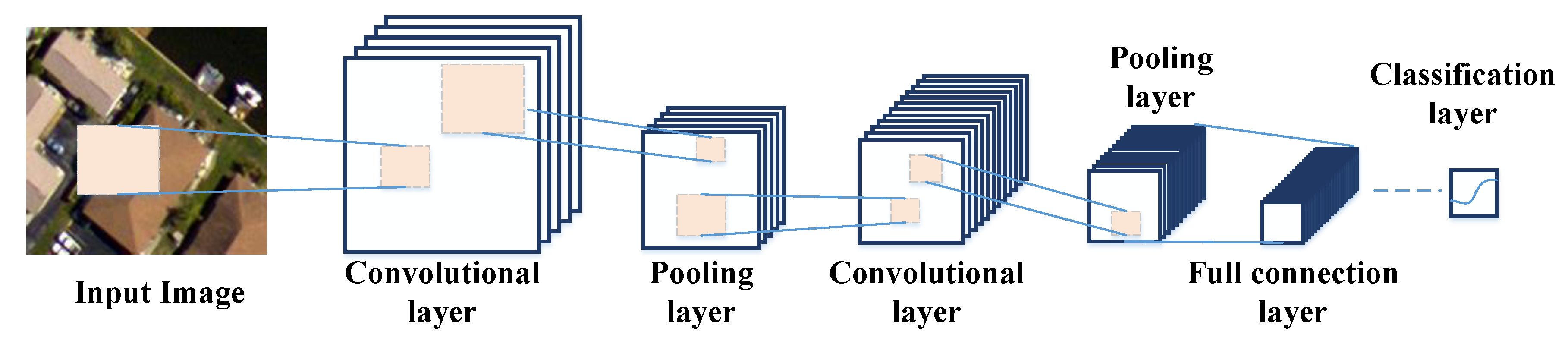
One of the most important deep learning models is the convolution neural network (CNN), which is widely used in VHR remote sensing image classification [37,38]. In general, traditional CNNs consist of five fundamental structures: the convolutional layer, non-linear mapping (NL) layer, pooling layer, full connection (FC) layer, and classification layer. The deep structure of CNNs is achieved by alternating a series of convolutional, NL, and pooling layers. The general CNN structure is shown in Figure 1.
In the convolutional layer, the output convolution features are obtained by convolving the trainable convolution kernel and the input sample or feature. Assume the input feature is , and l is the layer of the CNNs. The output convolution feature is expressed as [39]:
where * means the convolution operator, and and refer to the convolution kernel and biases, respectively.
After the convolutional layer, an NL layer follows to enhance the non-linear capability of the network. In this paper, the ReLU function is used as the non-linear activation function [40].
The purpose of pooling layer is to enhance the invariance of the learned feature by reducing the size of the features. Then, the output pooling features are rearranged as a feature vector and input to the FC layer. Finally, a softmax classifier is connected at the end of the CNNs for classification.
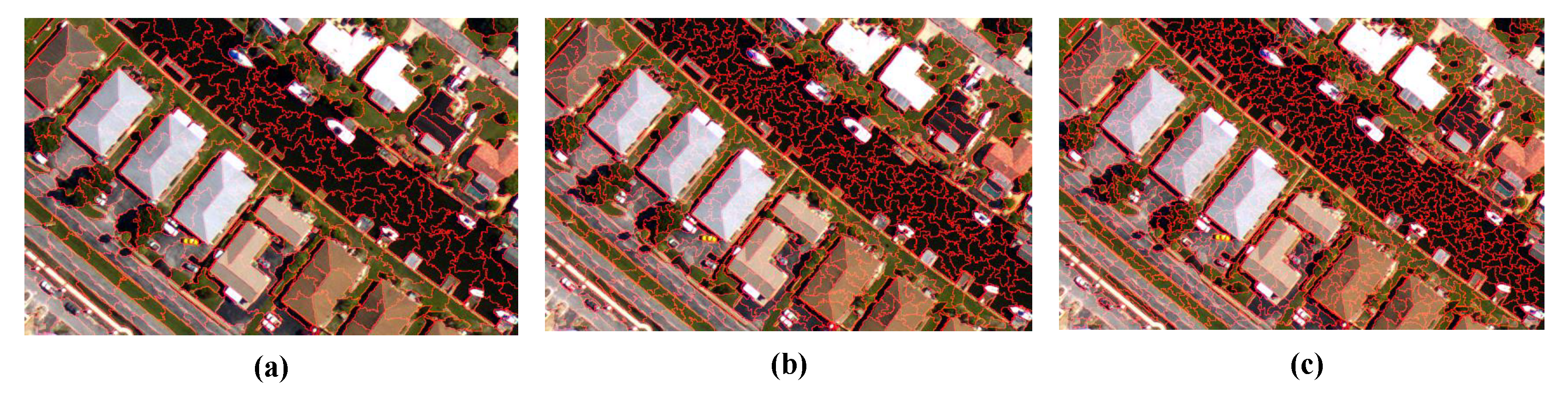
2.2. Superpixel Segmentation
Superpixel segmentation can adaptively segment the image into several homogeneous regions according to the intrinsic spatial structure [41]. Figure 2 shows the superpixel segmentation maps with different scales. In VHR remote sensing image classification, it is generally assumed that the pixels within each superpixel belong to the same category. Based on this assumption, Fang et al. [42] exploited the multi-scale superpixel features via multi-kernel learning. Jiao et al. [43] proposed a collaborative representation-based multiscale superpixel fusion method for HSI classification. Feng et al. [44] proposed a superpixel tensor sparse coding model for HSI classification. In our previous work, we proposed superpixel-based 3D CNNs for HSI classification [45]. A spatial feature map is extracted from HSI data to suppress the noisy pixels in classification results. Zheng et al. [46] proposed superpixel-guided training sample enlargement. Similar to our work, superpixel, which contains training samples belonging to only one class, was researched, and all the pixels within this superpixel were assigned to the class of the training samples it contained. All these pixels were used together with the initial training samples to train the classifiers. However, in superpixel segmentation, the mixed pixels may cause inaccurate positioning of land-cover boundaries, resulting in mislabeled samples that are added into the training set. Hence, in our method, we only assign the label to the center pixel of the superpixel to reduce false labeling.
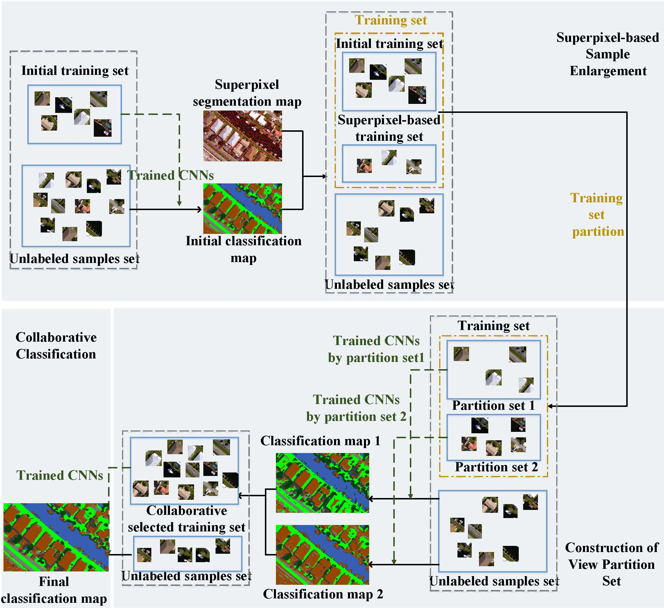
3. Proposed Method
In this paper, a hierarchical multi-view semi-supervised classification method for VHR remote sensing image classification is proposed. The proposed method mainly includes three stages: superpixel-based sample enlargement, the construction of a view partition set, and collaborative classification. In the first two stages, we will generate three classification maps from different views, which provide effective support for the final collaborative classification. The framework of the proposed method is shown in Figure 3.
3.1. Superpixel-Based Sample Enlargement
Initial training set is extracted by using a rectangular window on randomly selected pixels; D is the training sample and L is the label. The purpose of this section is to provide more reliable samples for subsequent view partition. Superpixel can segment the VHR remote sensing image into several homogenous regions. It is commonly assumed that the pixels within each superpixel share the same label. Hence, superpixel is always used in pseudo sample labeling. In fact, the rich details in VHR remote sensing images can interfere with extraction of object boundaries, because of such things as shadow occlusion. At the same time, due to the existence of the mixed pixels, the boundaries of the superpixel do not exactly match the object. To avoid the problem of mislabeled samples caused by the error extraction of boundaries, only the center pixel within each superpixel is selected and added into the training set. In the following, we will describe how to assign the pseudo label to the center pixels, in detail.
To assign a pseudo label to center pixels, the initial training set is used to train the CNNs, and the initial classification map can be obtained by the trained CNNs.
where means the CNNs trained by the initial training set, represents all unlabeled samples, is the predicted feature, and represents the predicted labels. According to the predicted label, the initial classification map is obtained.
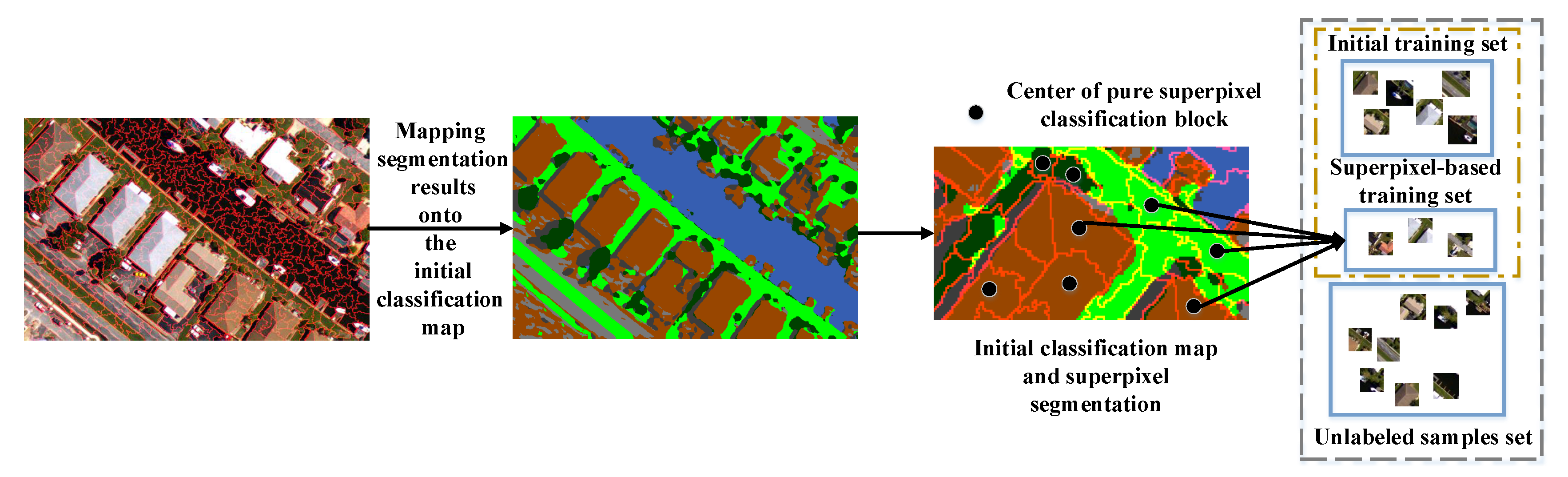
We perform superpixel segmentation on the VHR remote sensing image, and project the segmentation map onto the initial classification map. This process is shown in Figure 4. If the pixels within the superpixel have the same predicted label, the center pixel of this superpixel and its predicted label are added into the training set. In the proposed method, entropy rate segmentation [47] is adopted for superpixel segmentation. The other available superpixel segmentation methods can also be used here. The new training set , and consists of the selected unlabeled samples and their predicted labels.
3.2. Construction of a View Partition Set
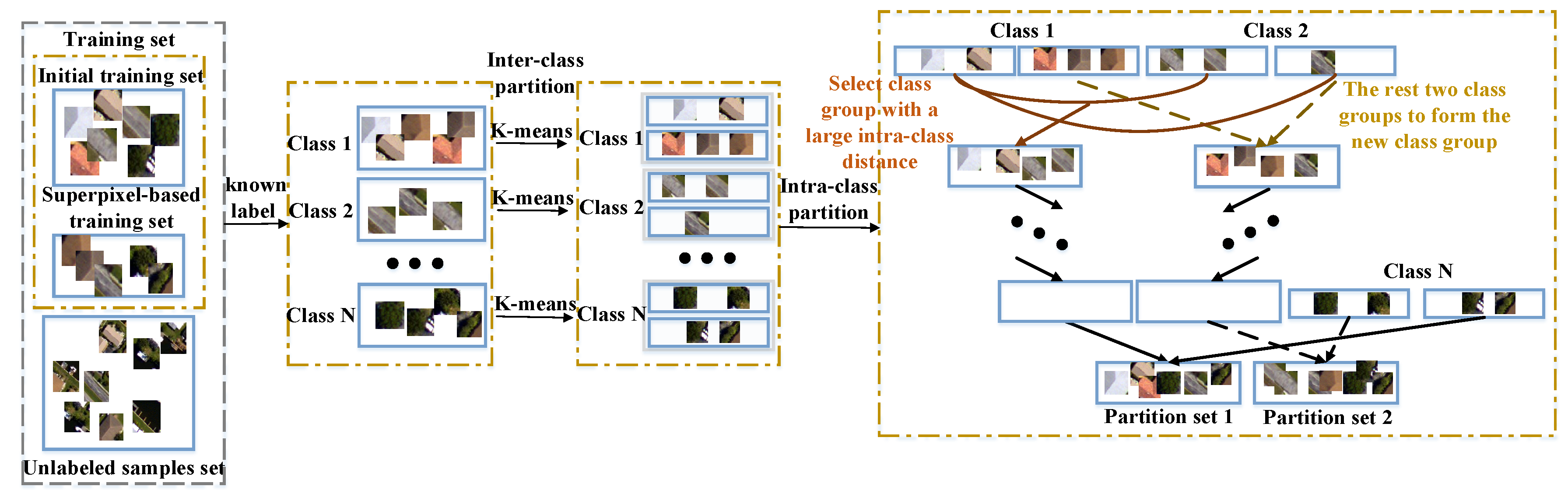
In this section, two partition sets are constructed from different views of the feature domain. The purpose of view partitioning is to make each partition set have the characteristics of inter-distinctiveness and intra-compactness; meanwhile, the correlation between different views is as low as possible. For this purpose, we designed a two-step partition method for view partitioning.
Through the trained CNNs in Section 3.1, the features of each training sample can be obtained. Assume the feature set of the training set is ; in the following, we will partition the feature set into two views. Figure 5 shows the view partitioning process. Notice that the partition process is only applied on the feature set of the training samples.
The proposed view partitioning process consists of two parts: intra-class partitioning and inter-class partitioning. The purpose of intra-class partitioning is to enhance the intra-compactness of each partition and the difference between the two partitions. According to the labels of the training samples, the feature set can be divided into N subsets; N is the class number, and . K-means [48] is an unsupervised cluster algorithm, which can achieve better clustering results with a lesser time cost. Hence, K-means is applied on each class for clustering, respectively. Since two view partition set is constructed in this section, each class is divided into two subsets, .
In the second part, the feature set is merged into two partition sets. The principle of the merging is to enlarge the inter-distinctiveness within each partition set. The merge process is carried out class-by-class. Assume the two partition sets are and . For Class 1 and Class 2, the corresponding intra-class partition feature sets are and . For each feature subset, the feature center is calculated via averaging the features of each feature subset, which are denoted as and . For the feature center , calculate its euclidean distances from and , and select a feature set with larger distance to join the partition . Assuming that and have a smaller difference, then , and the other two feature subsets are merged into partition . Similarly to the merging process of Classes 1 and 2, the feature subsets and will be merged as described above. Until the feature subsets are merged into the two partition sets, the view partitioning process is finished. Equation (4) shows the whole merging process.
The inter-class partition and inter-class merge process can enable us to obtain two partition sets with different views. Although the partitioning process is not completely orthogonal, the proposed method can make the two partition sets far apart.
The CNNs are trained via partition sets and , respectively. Two classification maps and with large differences can be obtained for the final decision.
3.3. Collaborative Classification
In Section 3.1 and Section 3.2, the classification maps of , , and were obtained, respectively. Since these three classification results were obtained from three different training sets, in this section, the three classification maps are combined for final classification.
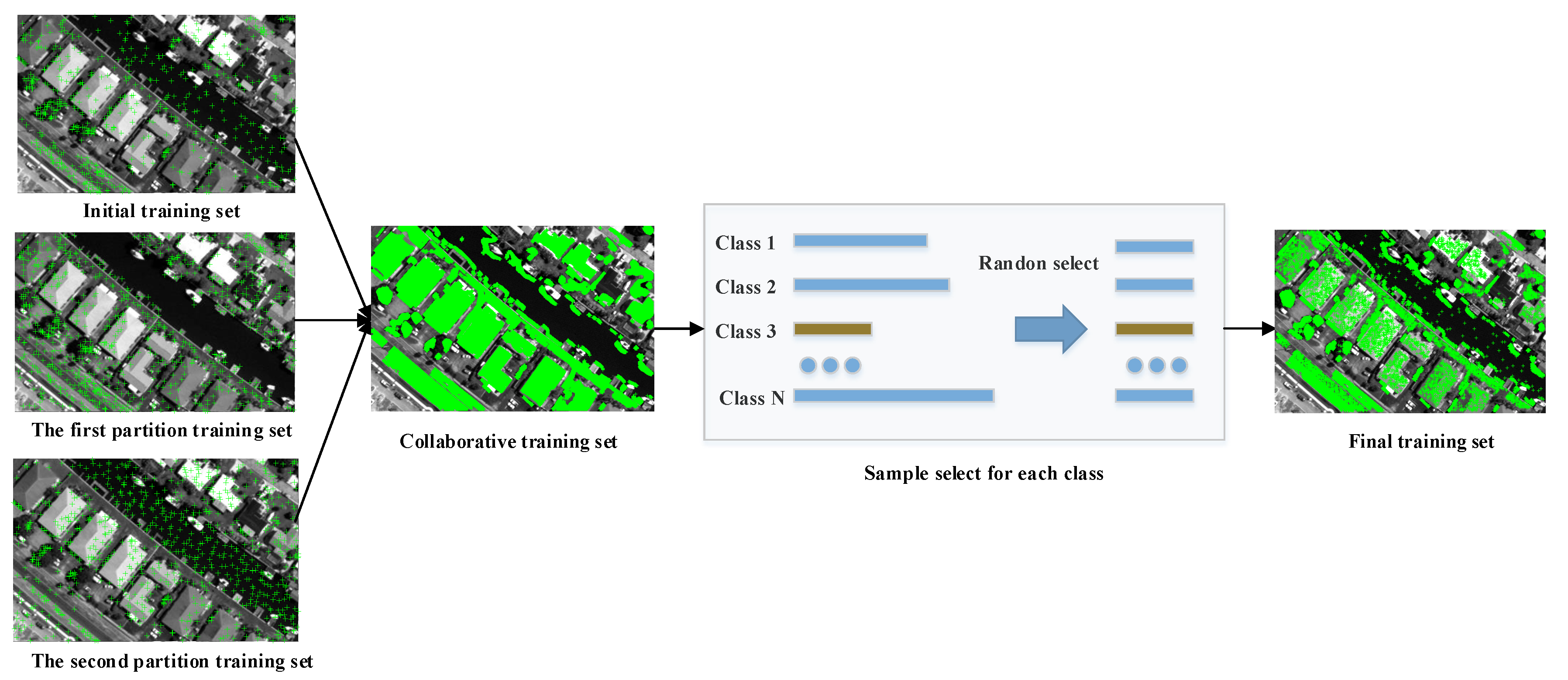
The collaborative classification process is shown in Figure 6. The final training set is constructed based on all the samples needed to be classified, which is irrelevant to the previously assigned pseudo-label. If the classification results of the sample in the three classification results are the same, then add this sample and its pseudo label to the training set. Because the training sets are large, computational complexity is increased; this also exacerbates the problems of sample imbalance. Therefore, we take the category with the fewest samples as the benchmark, and randomly select the corresponding number of samples from the other categories to form the new training set. Train the CNNs with the new training set and get the final classification result. The algorithm execution process of the proposed method is shown in Algorithm 1.
| Algorithm 1 Hierarchical multi-view semi-supervised learning for VHR remote sensing image classification. |
| Input: Training set and unlabeled testing set. |
| Output: Label predicted for the unlabeled samples. |
| Level 1: Superpixel-based sample enlargement |
| 1: Train the CNNs with training set and get the initial classification map . |
| 2: Segment the VHR image with superpixel segmentation method. |
| 3: Select appropriate unlabeled samples based on steps 1 and 2 to enlarged the training set . |
| Level 2: View partition |
| 4: According to the trained CNNs (step 1), obtain the feature set of training set . |
| 5: Intra-class partition for feature set by K-means. |
| 6: Intra-class partition for feature set by K-means. |
| 7: Train the CNNs with the two partition sets, respectively. |
| 8: Two classification maps and are obtained according to the trained CNNs (Step 7). |
| Level 3: Collaborative classification |
| 9: Select unlabeled samples with the same label prediction on , , to enlarge the training set. |
| 10: Train the CNNs with the new training set. |
| 11: Predict the labels of the unlabeled samples using the trained CNNs (Step 10). |
4. Experimental Results
4.1. Datasets
The following three VHR remote sensing images are used in our experiments.
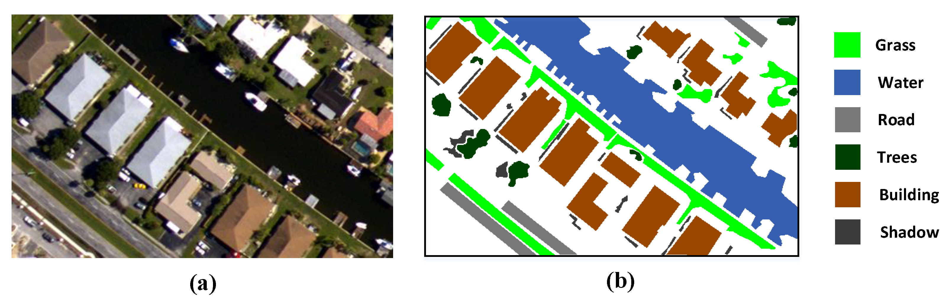
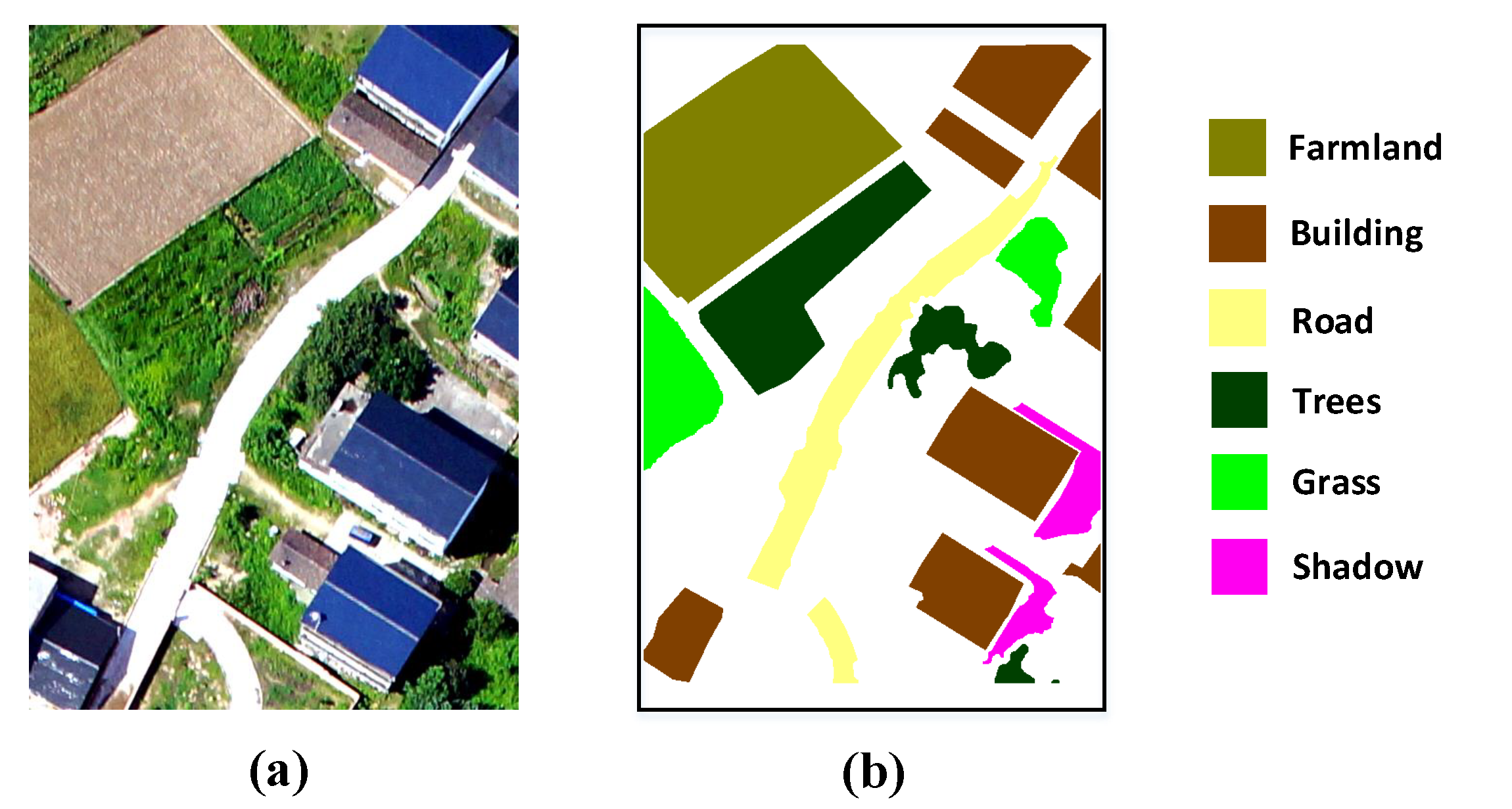
(a) Aerial data [49] was acquired by an ADS80 remote sensor on a plane. The spatial resolution of this scene is 0.32 m with three bands. The Aerial data are 560 lines by 360 samples; there are six classes available, including grass, water, road, trees, building, and shadow. The image data and its ground-truth map are shown in Figure 7a,b, respectively.
(b) JX_1 data were collected from UVA platform and Canon EOS 5D Mark II camera, and the flight elevation was 100 m. JX_1 data are a small subscene of JX image [49]. The size of the JX_1 data in pixels is with a spatial resolution of 0.1 m. JX_1 data have three bands with six classes available. Figure 8a,b show the image data and the ground-truth map, respectively.
(c) Pavia University data (http://www.ehu.eus//ccwintco/index.php?title=Hyperspectral_Remote_Sensing_Scenes.) were collected by the reflective optical system imaging spectrometer (ROSIS-3) optimal sensor on July, 8, 2002. The original HSI contains 115 spectral bands; after removing the noisy bands, only 103 bands are remained. This scene, with a size of , has a spatial resolution of 1.3 m. In this data set, nine classes are available for classification. The false color image data and its ground-truth are shown in Figure 9a,b, respectively.
4.2. Experiment Setup
In this paper, we compare the performance of our method with several start-of-the-art VHR remote sensing image classification methods, including a supervised classification method and semi-supervised classification methods.
The supervised classification method is a CNN [12]. CNNs are an effective feature extraction tool and have been widely used in VHR remote sensing image classification.
The semi-supervised classification methods include TSVM [25], semi-supervised MLR (SemiMLR) [26], a semi-supervised SAE (SemiSAE) [27], and a ladder network [28].
TSVM is an iterative algorithm, which incorporates the unlabeled samples into a training phase, and tries to search a much reliable separating hyperplane (in the kernel space).
SemiMLR combines the labeled samples and the unlabeled samples to improve the performance the multiple logistic regression classifier.
SimiSAE uses the large number of unlabeled samples to pre-train the unsupervised autoencoder, and fine-tunes the networks with the small labeled samples. The size of each hidden layer in the pre-trained autoencoder is: (for Aerial data and JX_1 data), and (for Pavia University data).
The ladder network is a recently proposed semi-supervised classification network. It consists of two encoders and one decoder, and during the training process, a supervised and an unsupervised cost are combined together for training. The supervised cost is to exploit the deep features of the labeled samples, and the unsupervised cost is to constraint reconstruction error of unlabeled samples. The architecture of the ladder network is (for Aerial data and JX_1 data), and (for Pavia University data).
In addition, to present the advantages of the proposed view partition method, we replaced the proposed two views with spectral feature and 2D Gabor feature [31] in the proposed framework, which is called spectral-spatial view in the following experiments.
The other parameters of the compared methods were set as the defaults from their papers. For the proposed method, the parameters were: the window size of the sample is , the superpixel number is 1000; and for CNNs, the first convolutional layer had 20 filters of size , the second convolutional layer had 40 filters of size . The full connection layer had 100 units, the iteration number was 1000, and the learning rate was set as . The numbers of the initial training samples are shown Table 1, and the average values of overall accuracy (OA) and average accuracy (AA), and the kappa coefficient, were used to evaluate the classification results.
4.3. Experimental Results on Aerial Data
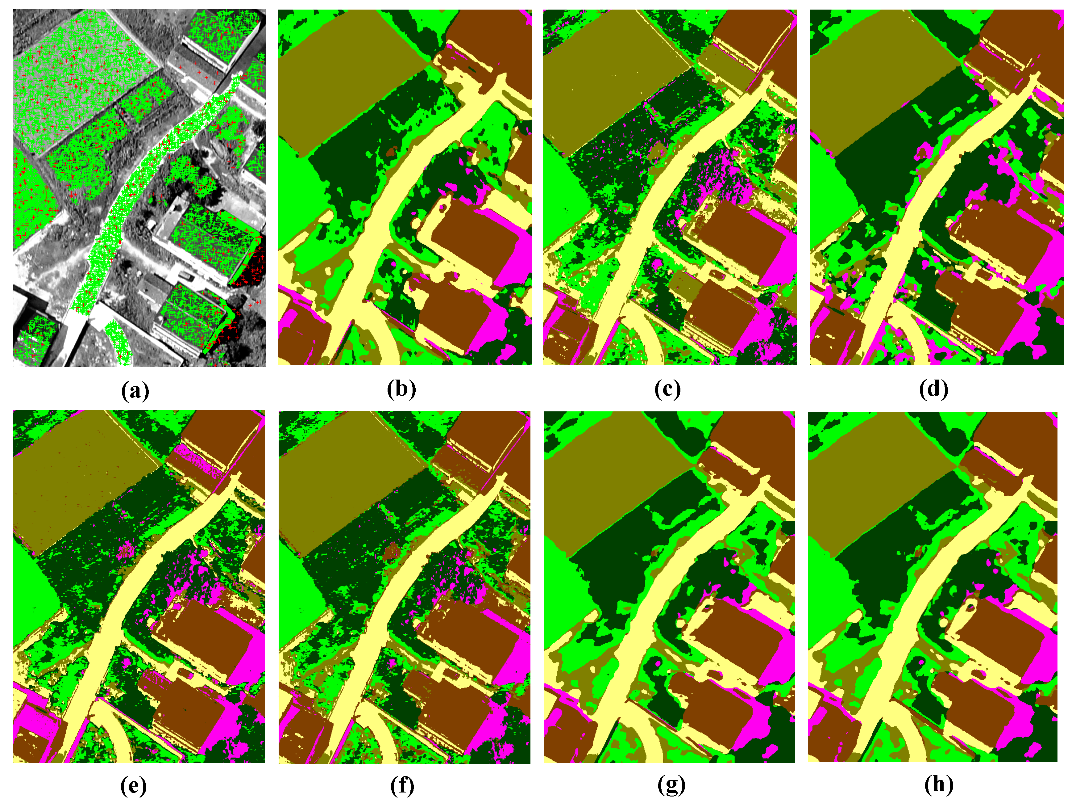
In this experiment, the performance of the proposed HMVSSL method was evaluated by using Aerial data. Figure 10 describes the classification results, and Table 2 tabulates the classification accuracies of the compared methods. The initial training and final training pixels are shown in Figure 10a with red and green markers, respectively. It is clear that the number of training samples increased significantly. In order to assess the label prediction accuracy for the selected unlabeled samples, we calculated the accuracy of these samples within ground-truth regions, and the accuracy is .
Compared with CNNs, the advantages of unlabeled samples are clearly revealed in the proposed method. The classification results of road and water have been improved significantly. Meanwhile, as can be shown from Table 2, the classification accuracies of road and water are increased and , respectively, and the OA value is increased by compared to CNNs. For other semi-supervised learning methods, TSVM has lower classification performance for road, trees, and shadow, and Table 2 also reports that the classification accuracy of road is only . SemiSAE has a lower classification performance in grass, and the OA value of grass is . The classification maps of semiSAE and the ladder network appear to be obviously noisy. The SemiMLR method shows obvious advantages in smooth areas, such as water, road, and building, and the classification accuracies of these three categories are higher than that of the proposed method. However, for the non-smooth regions and small details, e.g., trees and shadow, the classification accuracy is significantly reduced. The classification accuracies of trees and shadow are and lower than that of the proposed method. In the proposed HMVSSL method, the classification accuracy of each category is above , and there is no bias to one category. Because Gabor wavelet has obvious advantages for texture extraction, the spectral-spatial view gets higher classification accuracies on trees and roads. However, the redundancy between spectral and spatial views is large, and results in misclassified samples added into the training set. Hence the classification accuracy of spectral-spatial views is slightly lower than that of the proposed views, especially at the boundary of the building regions.
4.4. Experimental Results on JX_1 Data
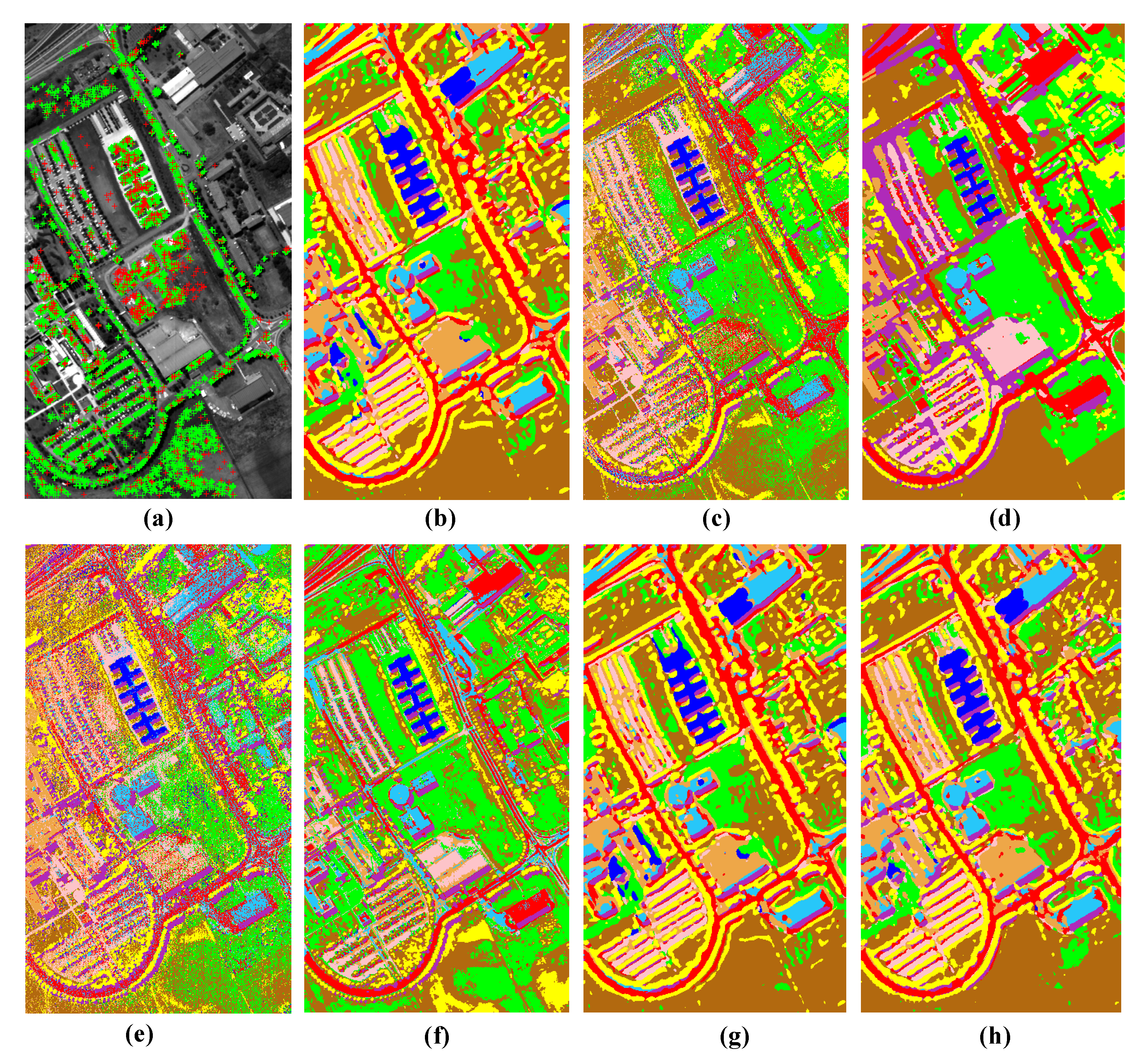
In this section, the classification performance is evaluated on JX_1 data. The classification maps and accuracies are illustrated in Figure 11 and Table 3, respectively. JX_1 data contains not only homogeneous regions with smaller intra-class differences, such as farmland, buildings, and roads, but also land-cover areas with large intra-class differences, such as trees and grass.
As can be seen from Figure 11, the compared methods show different classification performances for trees and grass. The classification maps of TSVM, SemiSAE, and ladder networks methods show obvious misclassifications within these two categories. In Table 3, the classification accuracies of grass (class 5) in these three methods are , , and ; meanwhile, for CNNs, SemiMLR, and the proposed method—, , and . CNNs, SemiMLR, and the proposed methods show better regional consistency. Although SemiMLR obtains a competitive OA value, its classification performance for small details are poorer, such as shadow ( for SemiMLR and for the proposed method). This case is similar to the former analysis on Aerial data. The proposed method achieves better performance in both visuals and classification accuracy. For the spectral-spatial view, the proposed method presented higher initial classification accuracies on the JX_1 data, and hence the probability that the same sample is mislabeled from the two views is small. Therefore, the spectral-spatial view also achieves better classification results. However, two independent views can obtain more high-reliability unlabeled samples, and therefore, the classification accuracy is slightly higher than that of the spectral-spatial view-based classification method.
4.5. Experimental Results on Pavia University Data
Pavia University data is a well-known HSI data which contains 103 bands. For CNNs and the proposed methods, PCA is performed first, and the first three PCs are maintained for the following classification. For the other methods, the input samples are extracted from the original HSI data. Pavia University data contains building and roads with rich details, and grass and soil areas with noisy information, which increases the difficulty of accurate land-cover interpretation.
Figure 12 and Table 4 present the classification maps and classification accuracies, respectively. TSVM and SemiSAE present classification maps with obvious salt-and-pepper noise, especially for SemiSAE—the classification accuracy is only . After the incorporation of the spatial information, CNNS, SemiMLR, and the proposed method show better anti-noise performance. Due to the use of unlabeled samples, the OA value obtained by the proposed method is higher than that of CNNs. For spectral-spatial view-based classification, reduced initial accuracy can lead to the probability of two views mislabeling the same sample. Hence, compared with CNNs, the increase of the classification accuracy is not significant. Therefore, when the accuracy of the initial classification is low, the independence of the two views has an important influence label decision process of the unlabeled samples. Hence, the proposed method performs better than the compared approaches in classification metrics, detail preservation, and region smoothness.
5. Discussion
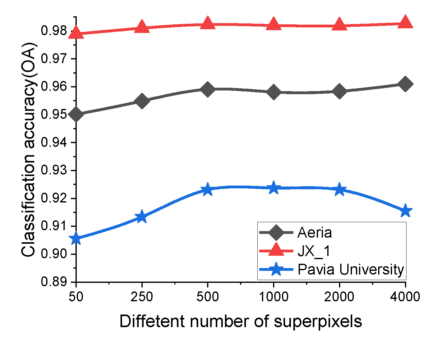
In the proposed method, the number of training samples is first enlarged by superpixel segmentation. The center pixel of the superpixel with “pure” classification is selected to enlarge the training set. Therefore, the superpixel number determines the correctness of the unlabeled sample selection. Figure 13 shows the classification results with different numbers of superpixels. The number of superpixel ranges from 50 to 2000. For Aerial data and JX_1 data, the effect of superpixel number on the classification accuracies is not obvious. But the situation is different for the Pavia University data. For Pavia University data, when the superpixel number is less than 500, the OA values are slight reduced, because a small number of unlabeled samples is selected. However, when the superpixel number is larger than 2000, the OA value also decreases due to the mislabeling of the unlabeled samples. Therefore, the classification evaluation metrics on the Pavia University data are more sensitive to the superpixel number.
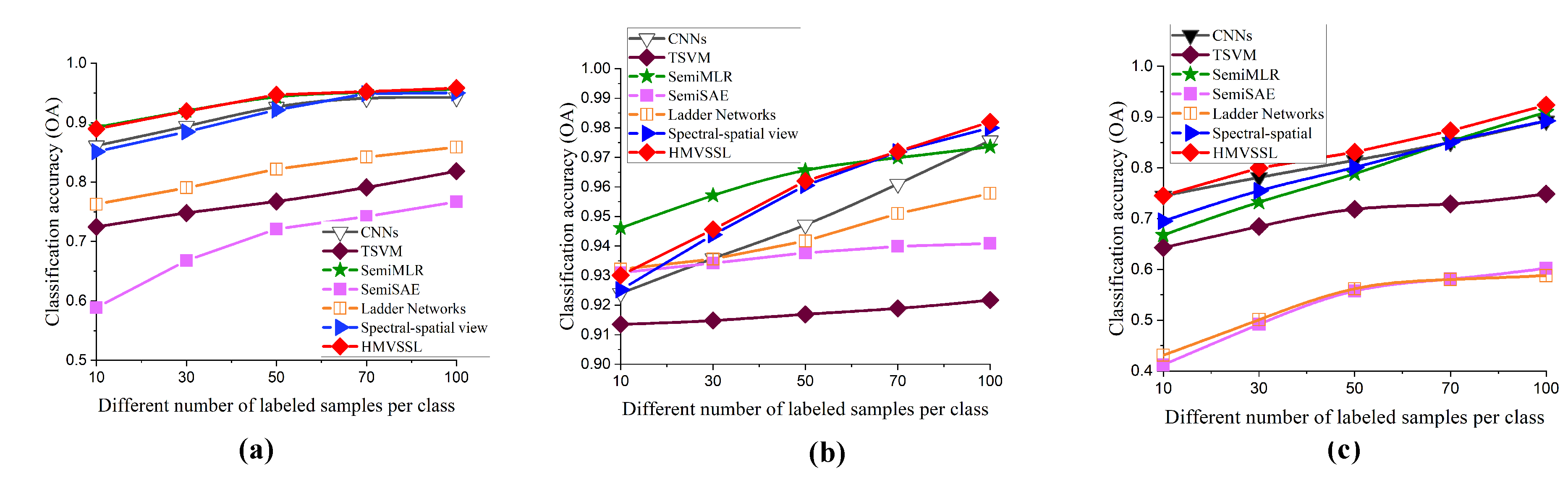
The other analysis is about the influence of the number of labeled samples on the classification accuracy. Figure 14 shows the classification performance of the compared and proposed methods. To further analyze the performance of these methods with the limited training sample, the number of labeled samples per class ranges from 10 to 100. Since the sample selection process is related to the initial classification map, the proposed method does not achieve good performance when the number of training samples is less than 30. However, as the number of training samples increases, the OA values are higher than that of the compared approaches. Therefore, the proposed method has superiority over the other methods when handling the problem of limited training samples.
6. Conclusions
This paper proposed a novel hierarchical multi-view semi-supervised learning framework for VHR remote sensing image classification. The proposed method consists of three levels: The first level is the enlargement of the training set, which may prevent the sharp reduction in the number of training samples after view partition. The second level is view partitioning, which can obtain two different views with the characteristics of inter-distinctiveness and intra-compactness. The designed view partitioning method can effectively improve the reliability of unlabeled sample selection. The third level is to combine the classification results of the previous levels for collaborative classification. Experiments were conducted on three VHR remote sensing datasets containing various land-cover classes, such as water, building, road, and grass. The experimental results verify the effectiveness of the proposed method compared to several state-of-the-art approaches.
There are two improvements that can be considered in future work. On the one hand, in the classification problem, most of the samples belong to “simple samples” that can be classified correctly. The remaining few samples are difficult to classify. These samples can be called “difficult samples.” In our work, the unlabeled samples are selected based on the correctly classified samples, and therefore, the improvement of classification performance is still limited for the “difficult samples.” Hence our further work is to effectively distinguish the difficult samples. On the other hand, the main contribution of the proposed method is view partitioning. Although self-training, co-training, and tri-training are all well-known semi-supervised classification frameworks, the reasons that we introduce view partitioning into co-training are: (1) Multi-view is always combined with co-training in most published multi-view-based remote sensing image classification methods. The main contribution of the proposed method is view-partitioning. In order to better understand to the background of view partitioning, we incorporate the proposed method by utilizing co-training. (2) For self-training, it mainly focuses on single-view learning. For tri-training, it usually uses the bootstrap sampling method to generate three different views. And for co-training, view construction is an important process. Hence, we evaluated the proposed method by utilizing co-training. In fact, the proposed view partitioning can also be utilized in self-training and tri-training methods. Perhaps that method can achieve better results.
Author Contributions
C.S. was primarily responsible for the original idea and experimental design. Z.L. and X.Y. contributed to the experimental analysis. P.X. provided important suggestions for improving the quality of the paper. I.B. provided suggestions for the revised paper. All authors have read and agreed to the published version of the manuscript.
Funding
This research was funded by the National Natural Science Foundation of China (61902313, 61701396, 61973250, 61801380) and the Natural Science Foundation of Shaan Xi Province (2018JQ4009).
Acknowledgments
The authors would like to express their gratitude to the editor-in-chief, the associate editor, and the reviewers for their insightful comments and suggestions.
Conflicts of Interest
The authors declare no conflict of interest.
References
- Bazi, T.; Melgain, F. Toward an optimal SVM classification system for hyperspectral remote sensing images. IEEE Trans. Geosci. Remote Sens. 2006, 44, 3374–3385. [Google Scholar] [CrossRef]
- Patra, S.; Bruzzone, L. A novel som-svm-based active learning technique for remote sensing image classification. IEEE Trans. Geosci. Remote Sens. 2014, 52, 6699–6910. [Google Scholar] [CrossRef]
- Li, W.; Prasad, S.; Fowler, J.E.; Bruce, L.M. Locality-preserving dimensionality reduction and classification for hyperspectral image analysis. IEEE Trans. Geosci. Remote Sens. 2012, 50, 1185–1198. [Google Scholar] [CrossRef] [Green Version]
- Xanthopoulos, P.; Pardalos, P.M. Linear Discriminant Analysis; Springer: New York, NY, USA, 2007; pp. 237–280. [Google Scholar]
- Shafri, H.Z.M.; Suhaili, A.; Mansor, S. The performance of maximum likelihood, spectral angle mapper, neural network and decision tree classifiers in hyperspectral image analysis. J. Comput. Sci. 2007, 6, 419–423. [Google Scholar] [CrossRef] [Green Version]
- Ham, J.; Chen, Y.C.; Crawford, M.M.; Ghosh, J. Investigation of the random forest framework for classification of hyperspectral data. IEEE Trans. Geosci. Remote Sens. 2007, 43, 492–501. [Google Scholar] [CrossRef] [Green Version]
- Pan, C.; Gao, X.B.; Wang, Y.; Li, J. Markov random field integrating adaptive interclass-pair penalty and spectral similarity for hyperspectral image classification. IEEE Trans. Geosci. Remote Sens. 2018, 57, 2520–2534. [Google Scholar] [CrossRef]
- Flores, E.; Zortea, Z.; Scharcanski, J. Dictionaries of deep features for land-use scene classification of very high spatial resolution images. Pattern Recognit. 2019, 89, 32–44. [Google Scholar] [CrossRef]
- Deng, C.; Liu, X.L.; Li, C.; Tao, D.C. Active multi-kernel domain adaptation for hyperspectral image classification. Pattern Recognit. 2018, 77, 306–315. [Google Scholar] [CrossRef] [Green Version]
- Benediktsson, J.A.; Palmason, J.A.; Sveinsson, J.R. Classification of hyperspectral data from urban areas based on extended morphological profiles. IEEE Trans. Geosci. Remote Sens. 2005, 43, 480–491. [Google Scholar] [CrossRef]
- Kang, X.D.; Li, S.T.; Benediktsson, J.A. Spectral-spatial hyperspectral image classification with edge-preserving filtering. IEEE Trans. Geosci. Remote Sens. 2014, 52, 2666–2677. [Google Scholar] [CrossRef]
- Chen, Y.S.; Lin, Z.H.; Zhao, X.; Wang, G.; Gu, Y.F. Deep learning-based classification of hyperspectral data. IEEE J. Sel. Top. Appl. Earth Obs. Remote Sens. 2014, 7, 2094–2107. [Google Scholar] [CrossRef]
- Cheng, G.; Li, Z.P.; Yao, X.W.; Guo, L.; Wei, Z.L. Remote sensing image scene classification using bag of convolutional features. EEE Geosci. Remote Sens. Lett. 2017, 14, 1729–1735. [Google Scholar] [CrossRef]
- Cheng, G.; Li, Z.P.; Han, J.W.; Yao, X.W.; Guo, L. Exploring hierarchical convolutional features for hyperspectral image classification. IEEE Trans. Geosci. Remote Sens. 2018, 56, 6712–6722. [Google Scholar] [CrossRef]
- Zhou, P.C.; Han, H.W.; Cheng, G.; Zhang, B.C. Learning compact and discriminative stacked autoencoder for hyperspectral image classification. IEEE Trans. Geosci. Remote Sens. 2019, 57, 4823–4833. [Google Scholar] [CrossRef]
- Chen, Y.S.; Jiang, H.; Li, C.; Ghamisi, P. Deep feature extraction and classification of hyperspectral images based on convolutional neural networks. IEEE Trans. Geosci. Remote Sens. 2016, 57, 6232–6251. [Google Scholar] [CrossRef] [Green Version]
- Mirzaei, S.; Hamme, H.V.; Khosravani, S. Hyperspectral image classification using non-negative tensor factorization and 3D convolutional neural networks. Signal Process. Image Commun. 2019, 76, 178–185. [Google Scholar] [CrossRef]
- Seydgar, S.; Naeini, A.A.; Zhang, M.M.; Li, W.; Satari, M. 3-D convolutional-recurrent networks for spectral-spatial classification of hyperspectral images. Remote Sens. 2019, 11, 883. [Google Scholar] [CrossRef] [Green Version]
- Qi, W.C.; Zhang, X.; Wang, N.; Zhang, M.; Cen, Y. spectral-spatial cascaded 3D convolutional neural network with a convolutional long short-term memory networks for hyperspectral image classification. Remote Sens. 2019, 11, 2363. [Google Scholar] [CrossRef] [Green Version]
- Zhao, W.Z.; Du, S.H. Learning multiscale and deep representations for classifying remotely sensed imagery. ISPRS J. Photogramm. Remote Sens. 2016, 113, 155–165. [Google Scholar] [CrossRef]
- Zhang, M.M.; Li, W.; Du, Q. Diverse region-based CNN for hyperspectral image classification. IEEE Trans. Image Process. 2018, 27, 2623–2634. [Google Scholar] [CrossRef]
- Cui, X.M.; Zheng, K.; Gao, L.R.; Zhang, B.; Yang, D.; Ren, J.C. Multi-scale spatial-spectral convolutional networks with image-based framework for hyperspectral imagery classification. Remote Sens. 2019, 11, 2220. [Google Scholar] [CrossRef] [Green Version]
- Lestner, C.; Saffari, A.; Santner, J.; Bischof, H. Semi-supervised random forests. In Proceedings of the IEEE 12th International Conference on Computer Vision, Kyoto, Japan, 29 September–2 October 2009. [Google Scholar]
- Arshad, A.; Riaz, A.; Jiao, L.C. Semi-supervised deep fuzzy C-mean clustering for imbalanced multi-class classification. IEEE Access 2019, 7, 28100–28112. [Google Scholar] [CrossRef]
- Bruzzone, L.; Chi, M.; Marconcin, M. A novel transductive SVM for semisupervised classification of remote-sensing images. IEEE Trans. Geosci. Remote Sens. 2006, 44, 3363–3373. [Google Scholar] [CrossRef] [Green Version]
- Li, J.; Bioucas-Dias, J.; Plaza, A. Semi-supervised hyperspectral image segmentation using multinomial logistic regression with active learning. IEEE Trans. Geosci. Remote Sens. 2010, 48, 4085–4098. [Google Scholar]
- Fu, Q.Y.; Yu, X.C.; Wei, W.P.; Xue, Z.X. Semi-supervised classification of hyperspectral imagery based on stacked autoencoders. In Proceedings of the Eighth International Conference on Digital Image Processing (ICDIP 2016), Chengu, China, 29 August 2016; Volume 10033, p. 10032B-1. [Google Scholar]
- Rasmus, A.; Berglund, M.; Honkala, M.; Valpola, H.; Raiko, T. Semi-supervised learning with ladder networks. In Advances in Neural Information Processing System 28 (NIPS 2015); 2015; pp. 2554–3456. Available online: http://papers.nips.cc/paper/5947-semi-supervised-learning-with-ladder-networks.pdf (accessed on 20 March 2020).
- Feng, Z.X.; Yang, S.Y.; Wang, M.; Jiao, L.C. Learning dual geometric low-rank structure for semisupervised hyperspectral image classification. IEEE Trans. Cybern. 2019, in press. [Google Scholar] [CrossRef] [PubMed]
- Wang, X.Q. Research on multi-view semi-supervised learning algorithm based on co-training. In Proceedings of the fifth International Conference on Machine Learning and Cybernetics, Dalian, China, 13–16 August 2006; pp. 1276–1280. [Google Scholar]
- Zhang, X.R.; Song, Q.; Liu, R.C.; Wang, W.N.; Jiao, L.C. Modified co-training with spectral and spatial views for semisupervised hyperspectral image classification. IEEE J. Sel. Top. Appl. Earth Obs. Remote Sens. 2014, 7, 2044–2055. [Google Scholar] [CrossRef]
- Romaszewski, M.; Glomb, P.; Chrolewa, M. Semi-supervised hyperspectral classification from a small number of training samples using a co-training approach. ISPRS J. Photogramm. Remote Sens. 2016, 121, 60–76. [Google Scholar] [CrossRef]
- Dai, D.X.; Gool, L.V. Ensemble projection for semi-supervised image classification. In Proceedings of the 2013 IEEE International Conference on Computer Vision, Sydney, NSW, Australia, 1–8 December 2013; pp. 2072–2078. [Google Scholar]
- Dai, X.Y.; Wu-Dias, X.F.; Zhang, L.M. Semi-supervised scene classification for remote sensing images: A method based on convolutional neural networks and ensemble learning. IEEE Geosci. Remote Sens. Lett. 2019, 16, 869–873. [Google Scholar] [CrossRef]
- Livieris, I.E. A new ensemble self-labeled semi-supervised algorithm. Informatical 2019, 43, 221–234. [Google Scholar] [CrossRef] [Green Version]
- Livieris, I.E.; Drakopoulou, K.; Tampakas, V.; Mikropoulos, T.; Pintelas, P. An ensemble-basedsemi- supervised approach for predicting students’ performance. In Research on e-Learning and ICT in Education; Springer: Cham, Switzerland, 2018; pp. 25–42. [Google Scholar]
- Mei, X.G.; Pan, E.; Ma, Y.; Dai, X.B.; Huang, J.; Fan, F.; Du, Q.L.; Zheng, H.; Ma, J.Y. Spectral-spatial attention networks for hyperspectral image classification. Remote Sens. 2019, 11, 963. [Google Scholar] [CrossRef] [Green Version]
- Meng, Z.; Li, L.L.; Jiao, L.C.; Feng, Z.X.; Tang, X.; Liang, M.M. Fully dense multi-scale fusion network for hyperspectral image classification. Remote Sens. 2019, 11, 2718. [Google Scholar] [CrossRef] [Green Version]
- Lecun, Y.; Bottou, L. Gradient-based learning applied to document recognition. Proc. IEEE 1998, 86, 11–2278. [Google Scholar] [CrossRef] [Green Version]
- Glorot, X.; Bordes, A.; Bengio, Y. Deep sparse rectifier neural networks. J. Mach. Learn. Res. 2010, 315–323. [Google Scholar]
- Zhang, Y.S.; Jiang, X.W.; Wang, X.X.; Cai, Z.H. Spectral-spatial hyperspectral image classification with superpixel pattern and extreme learning machine. Remote Sens. 2019, 11, 1983. [Google Scholar] [CrossRef] [Green Version]
- Fang, L.Y.; Li, S.T.; Duan, W.H.; Ren, J.C.; Benediktsson, J.A. Classification of hyperspectral images by exploiting spectral-spatial information of superpixel via multiple kernels. IEEE Trans. Geosci. Remote Sens. 2015, 53, 6663–6674. [Google Scholar] [CrossRef] [Green Version]
- Jia, S.; Deng, X.L.; Zhu, J.S.; Xu, M.; Zhou, J.; Jia, X.P. Collaborative representation-based multiscale superpixel fusion for hyperspectral image classification. IEEE Trans. Geosci. Remote Sens. 2019, 5, 7770–7784. [Google Scholar] [CrossRef]
- Feng, Z.X.; Wang, M.; Yang, S.Y.; Liu, Z.; Liu, L.Z.; Wu, B.; Li, H. Superpixel tensor sparse coding for structural hyperspectral image classification. IEEE J. Sel. Top. Appl. Earth Obs. Remote Sens. 2017, 10, 1632–1639. [Google Scholar] [CrossRef]
- Shi, C.; Pun, C.M. Superpixel-based 3D deep neural networks for hyperspectral image classification. Pattern Recognit. 2018, 74, 600–616. [Google Scholar] [CrossRef]
- Zheng, C.Y.; Wang, N.N.; Cui, J. Hyperspectral image classification with small training sample size using superpixel-guided training sample enlargement. IEEE Trans. Geosci. Remote Sens. 2019, 57, 7307–7316. [Google Scholar] [CrossRef]
- Liu, M.Y.; Tuzel, O.; Ramalingam, S.; Chellappa, R. Entropy rate superpixel segmentation. In Proceedings of the 24th IEEE Conference on Computer Visual and Pattern Recognition, Providence, RI, USA, 20–25 August 2011. [Google Scholar]
- Hartigan, J.A.; Wong, M.A. A K-means clustering algorithm. Appl. Stat. 2013, 28, 100–108. [Google Scholar] [CrossRef]
- Lv, Z.Y.; Zhang, P.L.; Benediktsson, J.A. Automatic object-oriented, spectral-spatial feature extraction driven by tobler’s first law of geography for very high resolution aerial imagery classification. Remote Sens. 2017, 9, 285. [Google Scholar] [CrossRef] [Green Version]
Figure 1.
Typical CNN structure with seven layers.

Figure 2.
Superpixel segmentation map: (a) Superpixel number is 500. (b) Superpixel number is 1000. (c) Superpixel number is 1500.
Figure 2.
Superpixel segmentation map: (a) Superpixel number is 500. (b) Superpixel number is 1000. (c) Superpixel number is 1500.

Figure 3.
Framework of the proposed method. The proposed method consists of three stages: (1) Superpixel-based sample enlargement, which is to enlarge the training set initially. (2) Construction of view partition set, which is to generate two independent partition views for high-reliable sample selection. (3) Collaborative classification. Combine the category prediction results of the previous stages for classification.

Figure 4.
Superpixel-based sample selection. Segment the VHR image with superpixel segmentation, and the center pixel of superpixel with “pure” classification is selected to enlarge the training set.
Figure 4.
Superpixel-based sample selection. Segment the VHR image with superpixel segmentation, and the center pixel of superpixel with “pure” classification is selected to enlarge the training set.

Figure 5.
The view partitioning process. Two independent view partition sets are constructed based on the training set.
Figure 5.
The view partitioning process. Two independent view partition sets are constructed based on the training set.

Figure 6.
Construction of the final training set based on the samples selected in the previous stages. The green markers are the positions of the selected training samples.
Figure 6.
Construction of the final training set based on the samples selected in the previous stages. The green markers are the positions of the selected training samples.

Figure 7.
Aerial data: (a) Image data. (b) Available ground-truth.

Figure 8.
JX_1 data: (a) Image data. (b) Available ground-truth.

Figure 9.
Pavia University data: (a) False-color map. (b) Available ground-truth.

Figure 10.
Classification results of the methods for Aerial data: (a) Selected training samples (red markers are the initial selected training points, and the green markers are the final selected training points). (b) CNNs. (c) TSVM. (d) SemiMLR. (e) SemiSAE. (f) Ladder network. (g) Spectral-spatial view. (h) HMVSSL (proposed).

Figure 11.
Classification results of the compared methods for JX_1 data: (a) Selected training samples (red markers are the initial selected training points, and the green markers are the final selected training points). (b) CNNs. (c) TSVM. (d) SemiMLR. (e) SemiSAE. (f) Ladder network. (g) Spectral-spatial view. (h) HMVSSL (proposed).

Figure 12.
Classification results of the compared methods for Pavia University data: (a) Selected training samples (red markers are the initial selected training points, and the green markers are the final selected training points). (b) CNNs. (c) TSVM. (d) SemiMLR. (e) SemiSAE. (f) Ladder network. (g) Spectral-spatial view. (h) HMVSSL (proposed).

Figure 13.
Classification results with different numbers of superpixels.

Figure 14.
Classification accuracies of the comparisons with different numbers of labeled samples per class: (a) Aeria data. (b) JX_1 data. (c) Pavia University data.
Figure 14.
Classification accuracies of the comparisons with different numbers of labeled samples per class: (a) Aeria data. (b) JX_1 data. (c) Pavia University data.


Table 1.
Numbers of the initial training and testing samples.
| Class | Aeria Data | JX_1 Data | Pavia University Data | |||
|---|---|---|---|---|---|---|
| Training | Testing | Training | Testing | Training | Testing | |
| 1 | 100 | 14,719 | 100 | 46,276 | 100 | 6631 |
| 2 | 100 | 37,022 | 100 | 45,278 | 100 | 18,649 |
| 3 | 100 | 5791 | 100 | 20,347 | 100 | 2099 |
| 4 | 100 | 4077 | 100 | 27,849 | 100 | 3064 |
| 5 | 100 | 3374 | 100 | 14,956 | 100 | 1345 |
| 6 | 100 | 3374 | 100 | 8019 | 100 | 5029 |
| 7 | 100 | 1330 | ||||
| 8 | 100 | 3682 | ||||
| 9 | 100 | 947 | ||||
| total | 1200 | 100,463 | 1200 | 162,785 | 1800 | 42,776 |
Table 2.
Classification accuracies of the compared methods on Aerial data.
| Class | CNNs | TSVM | SemiMLR | SemiSAE | Ladder Networks | Spectral- Spatial View | HMVSSL |
|---|---|---|---|---|---|---|---|
| 1 | 0.9948 | 0.9766 | 0.9808 | 0.2828 | 0.9811 | 0.9906 | 0.9963 |
| 2 | 0.9320 | 0.9421 | 0.9643 | 0.8356 | 0.7908 | 0.9401 | 0.9600 |
| 3 | 0.9168 | 0.0484 | 0.9698 | 0.9686 | 0.9444 | 0.9606 | 0.9418 |
| 4 | 0.9588 | 0.5013 | 0.7589 | 0.7331 | 0.6762 | 0.9674 | 0.9583 |
| 5 | 0.9306 | 0.8057 | 0.9750 | 0.8595 | 0.8866 | 0.9374 | 0.9410 |
| 6 | 0.9677 | 0.6037 | 0.7825 | 0.8459 | 0.8554 | 0.9766 | 0.9775 |
| OA | 0.9421 | 0.8182 | 0.9564 | 0.7669 | 0.8588 | 0.9501 | 0.9581 |
| AA | 0.9501 | 0.6463 | 0.9052 | 0.7542 | 0.8554 | 0.9621 | 0.9625 |
| Kappa | 0.9202 | 0.7444 | 0.9389 | 0.6896 | 0.8099 | 0.9311 | 0.9419 |
Table 3.
Classification accuracies of the compared methods on JX_1 data.
| Class | CNNs | TSVM | SemiMLR | SemiSAE | Ladder Networks | Spectral- Spatial View | HMVSSL |
|---|---|---|---|---|---|---|---|
| 1 | 1.0000 | 0.9992 | 0.9990 | 0.9923 | 0.9976 | 0.9985 | 0.9984 |
| 2 | 0.9548 | 0.8884 | 0.9943 | 0.9251 | 0.9922 | 0.9942 | 0.9990 |
| 3 | 0.9987 | 1.0000 | 1.0000 | 0.9996 | 1.0000 | 0.9975 | 0.9989 |
| 4 | 0.9545 | 0.8515 | 0.9794 | 0.9123 | 0.9192 | 0.9674 | 0.9598 |
| 5 | 0.9712 | 0.7967 | 0.8024 | 0.7904 | 0.7676 | 0.8970 | 0.9319 |
| 6 | 0.9759 | 0.9399 | 0.9428 | 0.9608 | 0.9337 | 0.9592 | 0.9694 |
| OA | 0.9757 | 0.9217 | 0.9736 | 0.9409 | 0.9587 | 0.9800 | 0.9820 |
| AA | 0.9759 | 0.9126 | 0.9530 | 0.9302 | 0.9350 | 0.9679 | 0.9747 |
| Kappa | 0.9691 | 0.9004 | 0.9664 | 0.9251 | 0.9474 | 0.9746 | 0.9771 |
Table 4.
Classification accuracy of the compared methods on Pavia University data.
| Class | CNNs | TSVM | SemiMLR | SemiSAE | Ladder Networks | Spectral- Spatial View | HMVSSL |
|---|---|---|---|---|---|---|---|
| 1 | 0.9143 | 0.6265 | 0.8085 | 0.6233 | 0.6373 | 0.9020 | 0.9385 |
| 2 | 0.9089 | 0.7522 | 0.9045 | 0.5186 | 0.3995 | 0.8946 | 0.9309 |
| 3 | 0.8833 | 0.7751 | 0.9252 | 0.7851 | 0.4493 | 0.8218 | 0.9419 |
| 4 | 0.9703 | 0.9367 | 0.9507 | 0.9076 | 0.8580 | 0.9768 | 0.9758 |
| 5 | 0.9985 | 0.9963 | 0.9948 | 0.9606 | 0.9896 | 1.0000 | 0.9970 |
| 6 | 0.7600 | 0.7447 | 0.9978 | 0.4983 | 0.8288 | 0.8039 | 0.8540 |
| 7 | 0.8211 | 0.8203 | 0.9910 | 0.7857 | 0.9195 | 0.9308 | 0.9361 |
| 8 | 0.8506 | 0.6070 | 0.8724 | 0.4723 | 0.6043 | 0.8786 | 0.8509 |
| 9 | 0.9905 | 0.9894 | 0.9958 | 0.9958 | 1.0000 | 0.9937 | 1.0000 |
| OA | 0.8923 | 0.7487 | 0.9097 | 0.6022 | 0.5878 | 0.8927 | 0.9237 |
| AA | 0.8997 | 0.8053 | 0.9378 | 0.7275 | 0.7429 | 0.9114 | 0.9361 |
| Kappa | 0.9905 | 0.6806 | 0.8829 | 0.5251 | 0.6080 | 0.8593 | 0.8995 |
© 2020 by the authors. Licensee MDPI, Basel, Switzerland. This article is an open access article distributed under the terms and conditions of the Creative Commons Attribution (CC BY) license (http://creativecommons.org/licenses/by/4.0/).
Share and Cite
MDPI and ACS Style
Shi, C.; Lv, Z.; Yang, X.; Xu, P.; Bibi, I. Hierarchical Multi-View Semi-Supervised Learning for Very High-Resolution Remote Sensing Image Classification. Remote Sens. 2020, 12, 1012. https://0-doi-org.brum.beds.ac.uk/10.3390/rs12061012
AMA Style
Shi C, Lv Z, Yang X, Xu P, Bibi I. Hierarchical Multi-View Semi-Supervised Learning for Very High-Resolution Remote Sensing Image Classification. Remote Sensing. 2020; 12(6):1012. https://0-doi-org.brum.beds.ac.uk/10.3390/rs12061012
Chicago/Turabian StyleShi, Cheng, Zhiyong Lv, Xiuhong Yang, Pengfei Xu, and Irfana Bibi. 2020. "Hierarchical Multi-View Semi-Supervised Learning for Very High-Resolution Remote Sensing Image Classification" Remote Sensing 12, no. 6: 1012. https://0-doi-org.brum.beds.ac.uk/10.3390/rs12061012
Note that from the first issue of 2016, this journal uses article numbers instead of page numbers. See further details here.