Article

Trends in the Stability of Antarctic Coastal Polynyas and the Role of Topographic Forcing Factors

1
Aerospace Information Research Institute, Chinese Academy of Sciences, Beijing 100094, China
2
School of Electronic, Electrical and Communication Engineering, University of Chinese Academy of Sciences, Beijing 100049, China
*
Author to whom correspondence should be addressed.
Submission received: 2 February 2020 / Revised: 17 March 2020 / Accepted: 18 March 2020 / Published: 24 March 2020

Abstract

:
Polynyas are an important factor in the Antarctic and Arctic climate, and their changes are related to the ecosystems in the polar regions. The phenomenon of polynyas is influenced by the combination of inherent persistence and dynamic factors. The dynamics of polynyas are greatly affected by temporal dynamical factors, and it is difficult to objectively reflect the internal characteristics of their formation. Separating the two factors effectively is necessary in order to explore their essence. The Special Sensor Microwave/Imager (SSM/I) passive microwave sensor has been making observations of Antarctica for more than 20 years, but it is difficult for existing current sea ice concentration (SIC) products to objectively reflect how the inherent persistence factors affect the formation of polynyas. In this paper, we proposed a long-term multiple spatial smoothing method to remove the influence of dynamic factors and obtain stable annual SIC products. A halo located on the border of areas of low and high ice concentration around the Antarctic coast, which has a strong similarity with the local seabed in outline, was found using the spatially smoothed SIC products and seabed. The relationship of the polynya location to the wind and topography is a long-understood relationship; here, we quantify that where there is an abrupt slope and wind transitions, new polynyas are best generated. A combination of image expansion and threshold segmentation was used to extract the extent of sea ice and coastal polynyas. The adjusted record of changes in the extent of coastal polynyas and sea ice in the Southern Ocean indicate that there is a negative correlation between them.

Graphical Abstract

1. Introduction

Polynyas are mesoscale phenomena that occur in the polar regions, and are important features of sea ice cover. The term refers to an area of open water in sea ice that remains ice free or covered by thin ice for a long time under weather conditions where sea water can freeze. Their horizontal scale ranges from 0.1 to 100 km, with areas in the range 10 to 105 km2 [1,2,3,4,5,6,7,8,9]. Polynyas are sensitive to climate change, and play an important role in air–sea interactions [6,9,10,11], halocline maintenance [3,11], and biodiversity [12,13,14,15,16]. The formation and expansion of a polynya is accompanied by salt precipitation during the freezing of sea water. The low temperature and high brine concentration produced in this process are an important source of dense polar water masses [17,18,19]. Polynyas play an important role in affecting the exchange of heat and moisture between the sea and the air [20,21,22]. The heat loss over thin ice (the polynya) can be several or even hundreds of times higher than the heat loss over thick ice (the sea ice) [23,24]. The open waters of polynyas are also important habitats for birds and marine mammals [8,25,26].
Depending on which mechanism forms and maintains polynyas in high latitude oceans, polynyas can be divided into open-ocean and coastal polynyas [1,7,27,28]. The formation of open-ocean polynyas is mainly due to a vertical circulation pattern, known as a "sensible-heat polynya" [1,27,29]. Due to continuous convective mixing, the heat from the upwelling deep warm water rises to the surface layer, which prevents the formation of sea ice. The surface-cooled seawater then sinks to the bottom of the ocean and is replaced by more rising warm water [27]. Due to the complexity of the influencing factors, the mechanisms behind the formation and maintenance of open-ocean polynyas are still not fully understood. The essence of a coastal polynya, in contrast, is a region where ice is constantly generated near the shore and is continuously carried out into the ocean by the action of local winds or ocean currents, which balances the loss of heat to the atmosphere and maintains the amount of heat in the open water at the same time [3,5,8,27,29,30]. The heat released into the atmosphere from coastal polynyas is derived from the heat that is lost from seawater in the form of "latent heat" during freezing. Therefore, this type of polynya is also called a "latent-heat polynya" [1,27,30]. Coastal polynyas in Antarctica play an important role in the production of highly saline and highly dense water, which has a profound impact on the formation of the Antarctic bottom water [18,19,31,32].
There are many factors that influence the formation and persistence of polynyas. Very recent studies have suggested that landfast sea ice (fast ice) plays an important role in the formation and variability of the polynyas [33]. Surface winds over Antarctica are closely related to the orientation and surface ice topography [34]. The Ross Shelf polynya (RSP) was inhibited by large icebergs, and the new polynyas formed downwind of the icebergs [35]. Within the ocean circulation, terrain obstacles can enhance the upward flow of warm deep water, which is an important factor in the formation and maintenance of polynyas [27]. Gordon [36] proposed that the formation of the Weddell Polynya in the Southern Ocean is the result of vertical convective mixing of ocean currents and surface-warming seawater caused by the underwater Maud Rise near the polynya. Alverson [37] used numerical methods to study the formation of polynyas under the influence of topographical factors, and found that local convection above seamounts is enhanced, and that the surface buoyancy flux can drive the convection of deep water. Based on the time scale involved, these influencing factors can be categorized as dynamic factors or persistent ones. The dynamic factors refer to temporary dynamical factors affecting the formation and maintenance of polynyas over a short period of time, including short-term variations in climatic conditions that are disturbance factors, such as the wind, surface ocean currents, and surface salinity. These factors have a large effect on studies of the secular variation in a polynya. The persistent factors refer to intrinsic persistent factors that act on polynyas for a long time; these include ocean thermodynamic processes [38,39], topography, and ocean dynamic processes [27,40,41]. Under the combined effect of these various factors, polynyas change constantly.
Thanks to the progress of remote sensing technology, it is now possible to use satellite sensors to monitor sea ice. However, coastal polynyas in the Southern Ocean are small-scale features that are difficult to monitor from satellite microwave radiometry. It is common to estimate the area of polynyas from SIC maps by using an ice concentration threshold. Passive microwave sensors are not restricted by the time of day, or influenced by clouds, and they have better space time continuity, which is important in the monitoring of sea ice in the polar regions. Markus and Burns proposed a polynya signature simulation method (PSSM) to estimate subpixel-scale coastal polynyas with satellite passive microwave data [42]. Several studies have generated polynyas detection and ice production estimation using polarization ratios from radiometer data [43,44]. A recent paper used a combination of the thermal infrared and passive microwave data to retrieve the sea ice production in polynyas [45]. At present, many kinds of SIC products are obtained from passive microwave remote sensing data [46,47], which provide sufficient data for monitoring polynyas. However, due to the influence of dynamic factors, some daily SIC products may show abrupt changes from one day to the next, and monthly products may vary greatly due to short-term climate anomalies in certain months. Additionally, the daily and monthly products can only provide information about polynyas over a short period of time, making it difficult to analyze the long-term stability of polynyas. What is more, current research on the factors affecting polynyas is limited to local areas and most studies are based on the results of simulation tests. The persistent factors are the decisive factors affecting the long-term stability of polynyas. Therefore, how to effectively remove the influence of dynamic factors and analyze the persistent factors affecting polynya formation and maintenance is an urgent problem that needs to be solved.
In the present study, we proposed a spatial-temporal smoothing strategy to obtain SIC products covering a period of one year (365 days) from which the dynamic factors were removed by making use of the SIC monitoring product for many years. A combination of the buffer clip and threshold segmentation was used to extract the area of sea ice and coastal polynyas. This paper analyzed the correlation between the formation and persistence of coastal polynyas and the local topography in the Southern Ocean, as well as changes in the long-term stability of the polynyas, which is affected by persistent factors. Finally, we analyzed how the topographical factors affected the stability of the polynyas over a multi-year period.

2. Materials and Methods

2.1. Data

The Special Sensor Microwave/Imager (SSM/I) and Special Sensor Microwave/Imager Sounder (SSM/IS) together form a passive microwave radiometric system, which has been carried onboard the Defense Meteorological Satellite Program (DMSP) satellites on the series of DMSP F-x satellites since 1987. These instruments operate in a near-polar orbit and the currently operating instruments are F15, F16, F17, and F18. These instruments measures dual-polarized microwave radiances at 19, 37, and 85 GHz and vertically polarized radiances at 22 GHz.
To analyze the formation and persistence of Southern Ocean polynyas, daily average SIC products and also seabed data for Antarctic were selected for use. The daily SIC products were acquired by the SSM/I and SSM/IS passive microwave satellites. These data are made available by the University of Hamburg, Germany (icdc.cen.uni-hamburg.de/), which uses the ARTIST Sea Ice (ASI) algorithm to illuminate the sea ice in different polarization modes using high frequency (the 85 GHz SSM/I and the 90 GHz SSM/IS channels) channels, with the brightness temperature polarization difference being obtained by inversion [48,49]. These channels have a considerably finer spatial resolution than the commonly used lower frequency channels. These SIC products are projected on to a polar stereographic grid that is true at a latitude of 70 degrees and has a resolution of 12.5 km [48]. The data selected for use covered the period from 1992 to 2018, and the study area consisted of the entire Antarctic region, including coastal polynyas and the Weddell Polynya.
The Antarctic seabed data was obtained from the Bedmap2 dataset (https://secure.antarctica.ac.uk/data/bedmap2/). Bedmap2 is a new gridded product generated by the British Antarctic Survey in 2013. It provides data for Antarctica south of 60°S [50]. Its spatial resolution is 1 km and it uses the WGS84 polar stereographic projection. Three variables of u10, v10, and si10 components of 10-m surface winds hourly data on single levels were obtained from Copernicus Climate Change Service (C3S) (2017): ERA5: Fifth generation of ECMWF atmospheric reanalysis of the global climate ( https://cds.climate.copernicus.eu/cdsapp#!/home) on October 20 1992 to 2018. These variables are measured at a height of 10 m above the surface of the Earth. The parameter u10 is the eastward component of the 10-m wind. The parameter v10 is the northward component of the 10-m wind. The parameter si10 refers to the calculation of a 3-s gust at each time step, and it has maintained its maximum value since the last post-processing. It has a resolution of 31 km with a Gaussian grid [51].

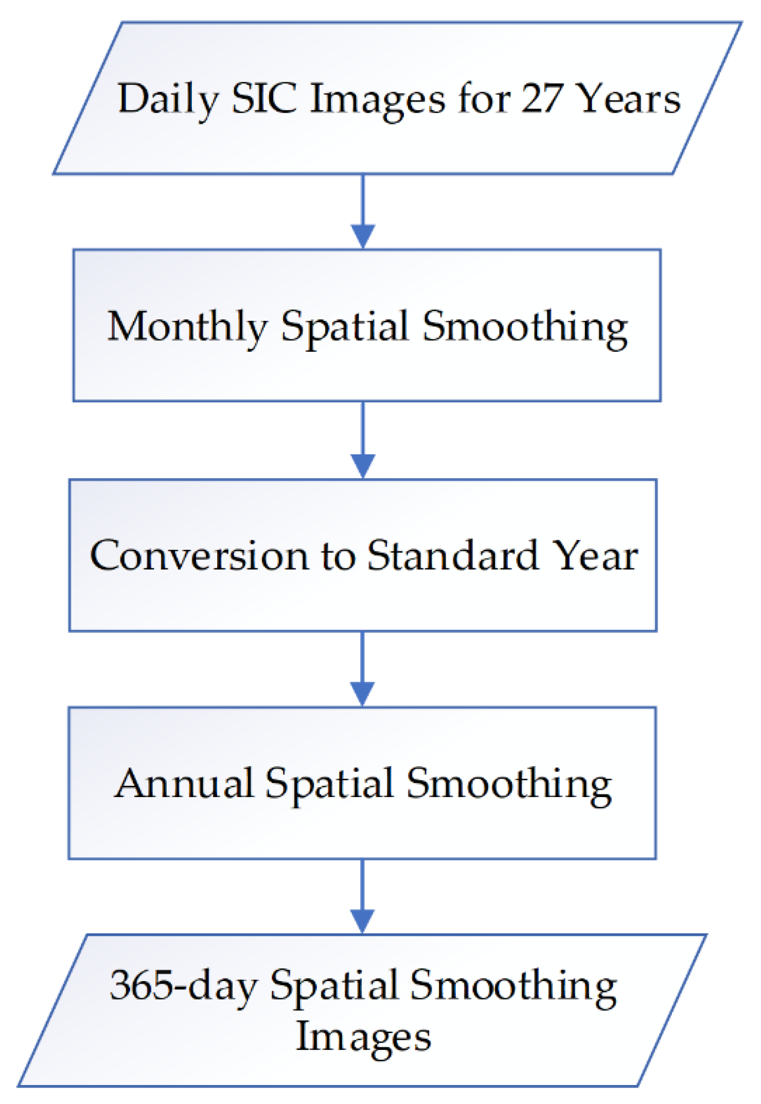
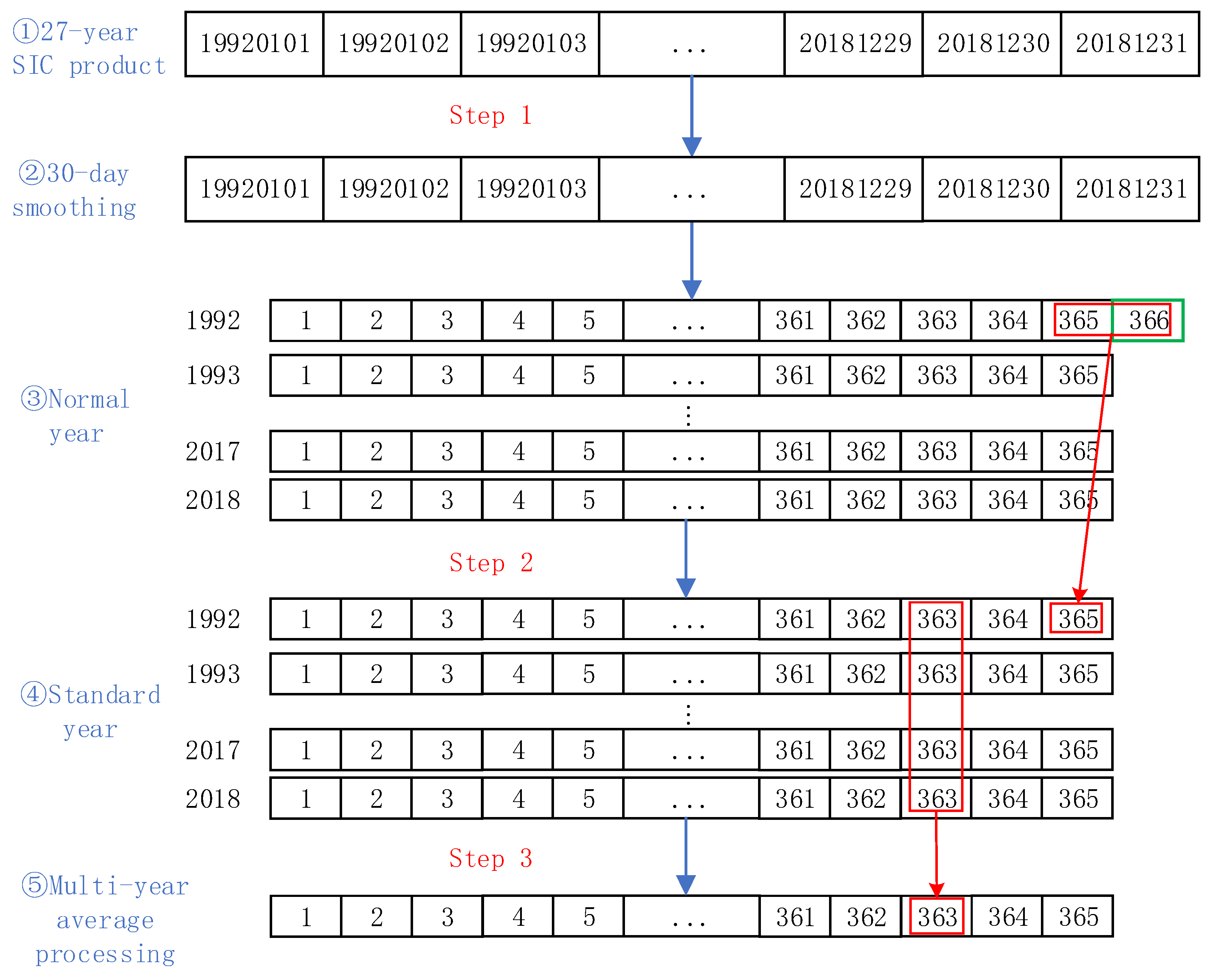
2.2. A Spatial Multi-Smoothing Algorithm

In order to remove the influence of dynamic factors, this study proposed a temporal spatial smoothing algorithm to smooth the passive microwave SIC products for many years. This algorithm is based on spatially filtered fields, and uses a combination of median filtering and mean filtering to remove dynamic factors from the SIC products. In addition, leap years have to be accounted for in order to unify the data format. The main idea of the algorithm is to perform multiple spatial smoothing processes in the time dimension for each pixel. The algorithm flow is shown in Figure 1.
This spatial smoothing processing can be divided into three main steps. Step 1 consists of monthly smoothing processing: That is, in order to remove the influence of dynamic factors over a period of 30 days, the value of each pixel is taken as the median value of the pixel in the 15 days prior to and 15 days after the day in question. Step 2 turns the year into a standard year: To deal with the leap year problem, the mean value of each pixel over two consecutive days is taken as the value of the previous day’s pixel. Thus, in the case of a leap year, the mean for day 365 is the average of days 365 and 366, such as the leap year of 1992 shown in Figure 2. Step 3 is the annual smoothing process: To remove the influence of annual random factors, the median value of a pixel value on the same day of the year over a period of 27 years calculated to obtain 365 days of annual averaged data. As shown in step 3 of Figure 2, the pixel-based median processing is performed on all the 363 days of 27 years to obtain the spatially smoothed SIC data of the 363th day. This algorithm can retain detailed information about multi-year data and data trends. By using this multiple spatial smoothing algorithm to obtain annual SIC spatial smoothing products that are not influenced by dynamic factors, subsequent analysis of the annual trends in sea ice and polynyas is possible.
Sea ice is at a maximum in the icing period in October and it begins to melt around the end of the month in the Southern Ocean. The time when the sea ice area is the largest is also the time when coastal polynyas are relatively stable. This study selected the data of October 20 as the time of maximum SIC in winter. Figure 3 shows the comparison results of the SIC processed by the spatial smoothing algorithm and pixel-based averaging. Figure 3a represents the spatially smoothed annual SIC product on October 20 for the data of 27 years; Figure 3b shows the result of the pixel-based averaging process for the October 20 data for each of the 27 years, as a comparison. The edges of the SIC shown in Figure 3b are more blurred while Figure 3a can clearly show the details of the SIC.

2.3. Extraction of Polynyas and Sea Ice

The threshold segmentation method can effectively extract targets from different gray-scale ranges and is applicable to the extraction of polynyas from SIC products. Polynyas are non-linear areas of open water or thin ice up to 0.3 m thick. The effectiveness of the 75% ice concentration threshold was determined by interactive analysis of the experimental winter images. For the extraction of polynyas and sea ice regions, this paper used the threshold segmentation method. Pixels with ice concentration values less than or equal to 75% were classified as polynya and where the ice concentration is 20% or greater classified as sea ice [35]. Specifically, the Antarctic continental margin was extracted firstly for the extraction of coastal polynyas, and then a 15-pixel buffer along the outside of this line was constructed; areas with this buffer with values of less than 75% were then considered to be the coastal polynyas extent. Denoising treatment was carried out on the extracted polynyas and sea-ice areas. In addition, there are two ice floes that persist for many years in the Antarctic coastal areas that have low SIC in the inversion of the SIC products (marked with two black circles in Figure 3a). In order to avoid being mistakenly identified as polynyas, these two areas were masked.

3. Results and Analysis

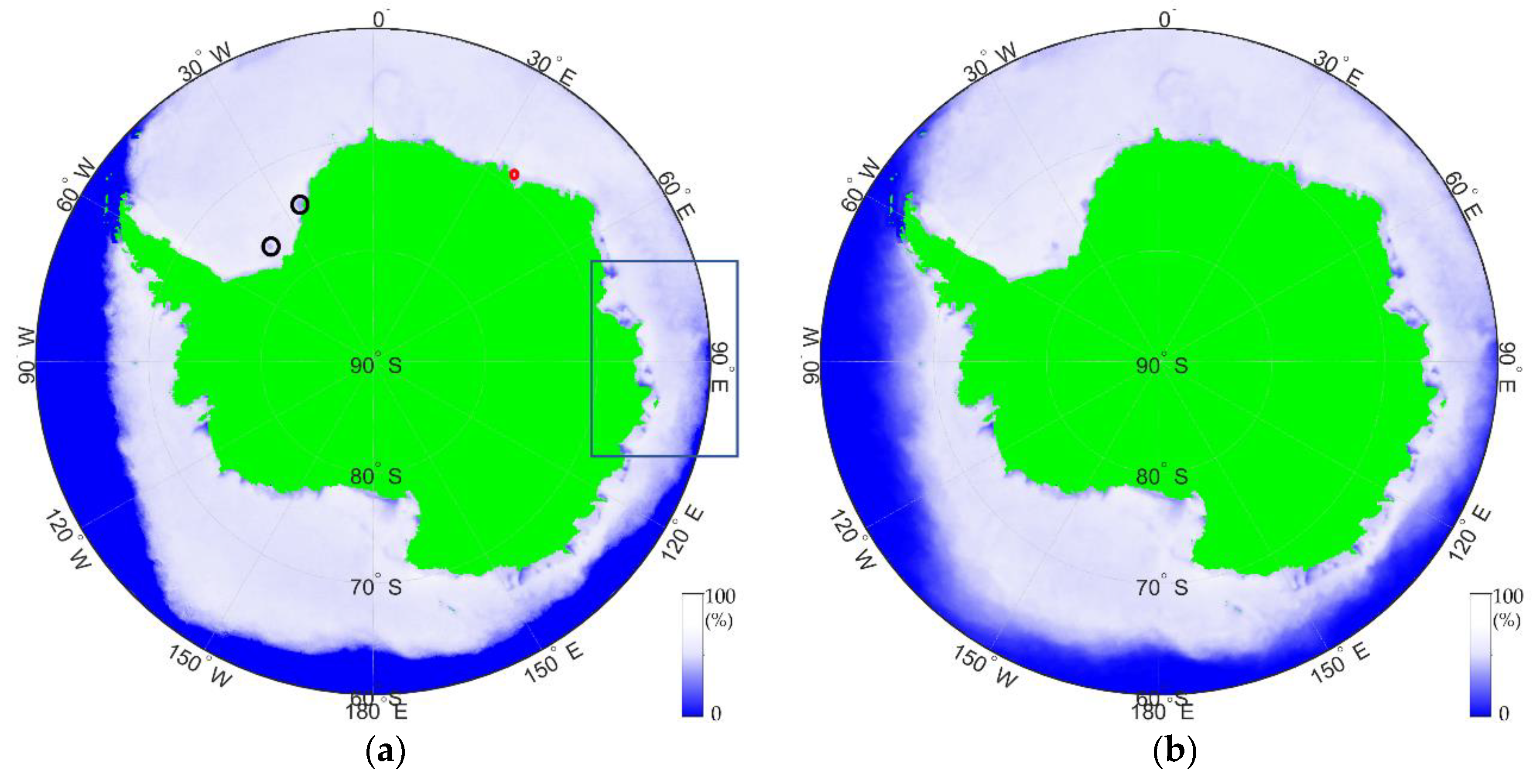
3.1. Comparison of Smoothing Results

To verify the effectiveness of the spatial multi-smoothing algorithm, the annual spatially smoothed sea ice extent for a period of 27 years was calculated in Figure 4. As a comparison, the annual averaged SIC data for the same date for 27 years on a pixel-by-pixel basis was used to calculate the sea ice extent, which is shown as the blue dotted line in Figure 4. Additionally, the sea-ice extent was calculated using the original data every five years (1992, 1997, 2002, 2007, 2012), with 2017 and 2018 used as a reference. A comparison of the percentages for a point with low SIC on October, obtained using the two different methods, is given in Figure 5. The position of this point is marked with a red circle in Figure 3a.
It can be seen from Figure 4 that the sea ice extent obtained by the spatial smoothing algorithm is basically the average of the original sea ice extent for the 27-year period. However, the sea ice extent obtained using the average pixel values is generally much higher. This is due to the fact that the average processing result based on pixels has a great influence on the area of low ice concentration (especially in the edge area of SIC), which has a large impact on the stability of the SIC values in several of the years shown. It can also be seen that the Antarctic sea ice extent in 2017 and 2018 was lower than in previous years.
By comparing the October sea ice percentages for one pixel point obtained using the two methods (Figure 5), it can be seen that the values obtained by spatial smoothing are less volatile than those obtained using the pixel-by-pixel averages. In the case of the former, the changes are more stable and the sudden changes in sea ice values on individual days are not present, which greatly reduced the impact of sea ice mutation caused by changes in dynamic factors, such as the short-term climate.

3.2. Stability Analysis of the Coastal Polynyas

Lindsay observed a distinctive halo of low ice concentration above Maud Rise [52]. There is a more obvious halo around the coast of the Antarctic continent. Due to the influence of the Antarctic continental wind, most of the coastal polynyas are adjacent to the mainland. The persistent factors influencing the formation and persistence of Antarctic polynyas have a strong correlation with the local seabed topography. In the Antarctic, there is often a rapid increase in depth at the beginning of the continental shelf slope, which can be considered a seabed topographic threshold. There is also a well-demarcated halo that follows the boundary between the area of low coastal ice concentration and the thick ice close to the shore (Figure 6). In addition, we found that the outer edge of the area of low coastal ice concentration in the Antarctic basically coincides with the direction of the outer contour of the local seabed topographic threshold. This paper used the SIC products (the gradient-enhanced data of the smoothing SIC products on October 20 using 27-year SIC products) and the Antarctic bedmap2 seabed data to extract the outer edge of the area of low coastal ice concentration and the local seabed topographic threshold. Using the Antarctic SIC (Figure 6a) and the Antarctic seabed elevation (Figure 6b) as the background, the outer edge of the area of low coastal ice concentration (the yellow line) and the edge of the seabed topographic threshold (the red line) are shown as superimposed in Figure 6a,b. As shown in Figure 7, this study analyzed the distance between the two edge lines. In total, 1000 sampling points were uniformly selected with black point A as the starting point and black point B as the end point from the two curves, and the data was standardized for z-scores, respectively. The small picture in Figure 7 is the distance between the edge of the seabed topographic threshold in Maud Rise and the halo appearing on its surrounding sea surface.
Figure 6a,b show the extracted outer edges of the low coastal ice concentration areas and the seabed. The overall fit for the two edges is highly consistent, especially between about 30°W to 150°E (in the clockwise direction). In contrast, the level of agreement between about 150°E to 60°W (in the clockwise direction) is relatively low. This is mainly due to the smaller coastal terrain gradient in this area, coupled with the influence of the wind and other factors, which results in the occurrence of polynyas directly above the shelf area. The outer edge of the low ice concentration area within the black rectangular frame does not coincide with the contour making the seabed shelf edge. However, the area of low ice concentration located directly above the abrupt change in the seabed has a halo in it, which is highly consistent with the abrupt change in the depth of the seabed. What is more, as shown in Figure 6a, the Weddell Polynya, marked by the green rectangular frame, is located at about 0°E away from the Antarctic continent, and the outer edge of the polynya or the halo [52] of low ice concentration that occurs there is highly consistent with the curvature of the outer contour of the Maud Rise on the seabed. These areas of low ice concentration are also the sites where the formation of polynyas is most likely to occur [24,30,53].
To analyze the correlation between the outer edge of the low coastal ice concentration and the edge of the seabed topographic threshold, the distance was calculated between the two curves in Figure 7. The abscissa is a mark that sorts the 1000 sample points by the sequence from the start point A to the end point B. The ordinate is the distance between the corresponding sampling points on the two curves, which is normalized by the Z-score. It can be seen from Figure 7 that the distances corresponding to sampling points 0–430 (54°W–98°E) are almost all less than 0, and the similarity between the two curves is higher than 99.5%. The distances corresponding to sampling points 0–658 (54°W-173°E) are generally less than 0; the similarity between the two curves is higher than 96.5%, and the overall similarity is greater than 70.6%. The distance between the two curves at Maud Rise is less than 0 and the similarity reaches 100% here. In short, the low coastal ice concentration edge and the seabed topographic threshold are highly consistent between 54°W and 173°E (in the clockwise direction). The coincidence between them is lower between 173°E and 65°W (in the clockwise direction), where the terrain is gentler. The correlation between the occurrence of polynyas and the local seabed topography is further discussed and analyzed from the horizontal and vertical perspectives in Section 3.2.1 and Section 3.2.2, respectively.

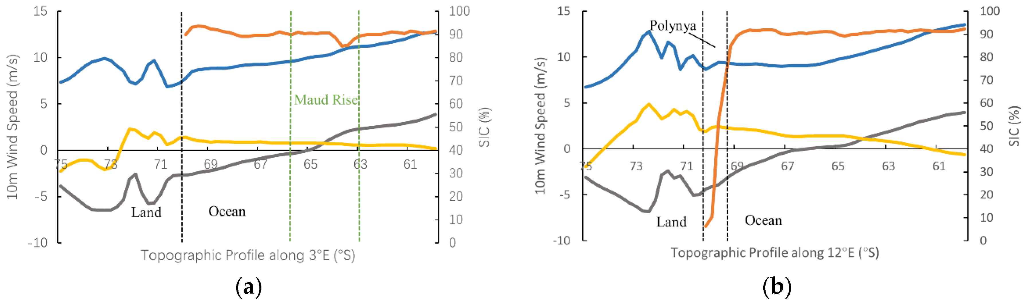
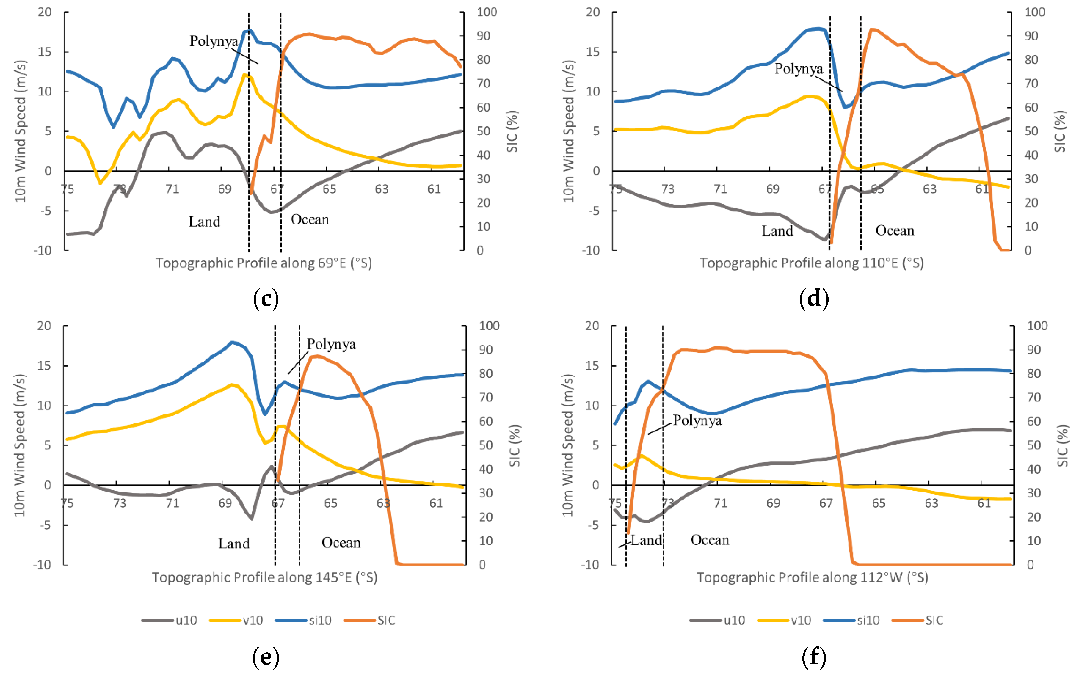
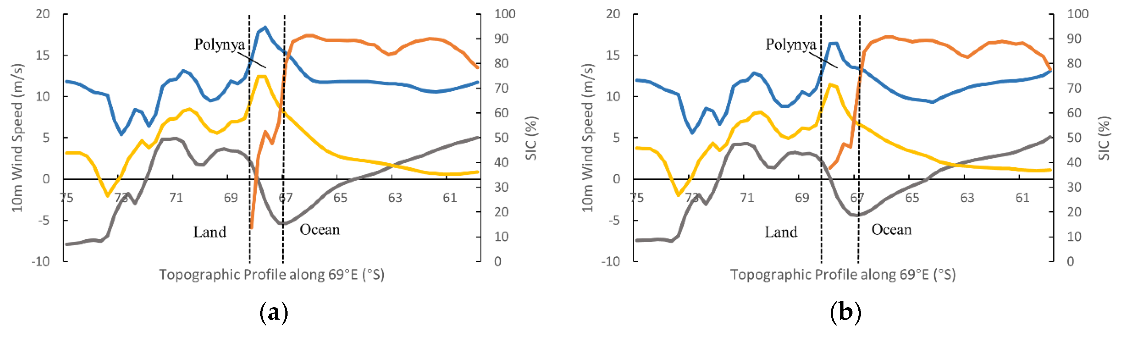
3.2.1. The Relationship Between Coastal Polynyas and Topography

Antarctic coastal polynyas are formed by the divergence between ice movements caused by prevailing winds or ocean currents, and most polynyas are covered by thin ice [24,30,53]. The horizontal distribution of the Southern Ocean Coastal Polynyas is inseparable from the topography of the local seabed. In this study, we conducted a statistical analysis of the horizontal distribution of the Southern Ocean Coastal Polynyas and its relation to the bed elevation.
To carry out this analysis, we used the topographic data of the Antarctic from the bedmap2 dataset and the spatially smoothed SIC data for October 20. First, the SIC data with dynamic factors removed were projected on to the WGS84 polar stereo projection, and the spatial resolution was resampled to 1km*1km using bilinear interpolation, which was consistent with the projection and spatial resolution of the seabed data in bedmap2. Then, the coastal polynyas, which had been resampled, were extracted from the spatially smoothed SIC data for October 20 using the threshold segmentation method. Finally, this paper extracted the seabed data for the extracted polynya areas and counted the number of pixels in the polynya that corresponded to different elevation values. The results are showing in the Figure 8 and Table 1.
It can be seen that almost all of the coastal polynyas correspond to areas that are between −1200 and 0 m above sea level and 88.81% of the polynyas correspond to the bed elevation range −800 to 0 m. There are two peaks in the distribution of coastal polynyas, ranging from −800 to −550 m and −500 to −150 m, respectively.
The distribution of the Southern Ocean polynyas is also closely related to the vertical profile of the local seabed, which mainly occurs in the area where the seabed changes abruptly. In particular, the appearance of polynyas near the Antarctic landmass is significant, and these polynyas occur closer to where this change in the seabed occurs. However, due to the influence of factors, such as the slope of the terrain, the ice sheet in some areas is not located at the edge of the area of this abrupt change. Coastal polynyas are usually distributed along the outer edge of the Antarctic continent due to the wind and other factors, which causes the position of some polynyas to be slightly offset and for them to appear in the surrounding area. Figure 9 shows the distribution of coastal polynyas on slope and wind speed. The wind speeds in Figure 9b represents the averaged values of the si10 variable from October 20 1992 to 2018. The black lines show the distribution of coastal polynyas in Figure 9.
In order to analyze the distribution of the polynya in relation to the topographic profile of the local seabed, this paper performed a topographical profile analysis of the spatially smoothed SIC data on 20 October after re-sampling and the Antarctic seabed data. According to the distribution of the polynyas and the distance of the two curves, we selected six representative meridional sections (a to f) in the SIC data in order to display the sea ice and the bed elevation. The locations of the six meridional sections are at 3°E, 12°E, 69°E, 110°E, 145°E, and 112°W, as shown in Figure 9a. Section (a) passes through the Maud Rise, and sections (b–e) pass through a polynya where the seabed changes abruptly.
This study further extracted the bed elevation and sea ice information for each meridional section, removing the Antarctic continent from the sea ice data, and the following cross-sectional view was used to analyze the distribution of the polynyas within the topographic section (Figure 10). The abscissa represents the latitude, the main ordinate represents the bed elevation, and the secondary ordinate represents the percentage of SIC (the percentage of SIC was calculated in the oceanic region, and the region of the Antarctic continent was ignored). The blue line represents the value of bed elevation, and the orange line represents the value of SIC.
A plot of the SIC against the topographical profile is shown in Figure 10. The profile (Figure 10a) passes through the outer edge of the Maud Rise, where the terrain is rapidly descending. There is often a polynya or halo located nearby in the Weddell Sea, and the SIC values within the halo are lower than the surrounding values. The positions of the polynyas in Figure 10b,c are exactly where the local seabed begins to drop rapidly; the polynyas shown in Figure 10d,e occur before the sudden drop in the seafloor. Coastal polynyas in the Southern Ocean are distributed along the edge of the ice sheet. In Figure 10c,d, this edge basically follows the topography of the local seabed. However, the edge of the ice sheet near the shore shown in Figure 10d,e slightly deviates from the local seabed topographic threshold, and its edge more closely follows the Antarctic landmass than the seabed topography. Therefore, the locations of the polynyas in this area are correspondingly closer to the Antarctic. However, the edge of the polynyas near the ocean is still consistent with the contours of the local terrain. In contrast, the location of the polynyas in Figure 10f is far from the steep part of the terrain and the slope here is relatively gentle. There is an area of flat land in the middle of the local terrain, which is exactly where the edge of the ice sheet is located, and the polynyas are distributed along the ice sheet here.

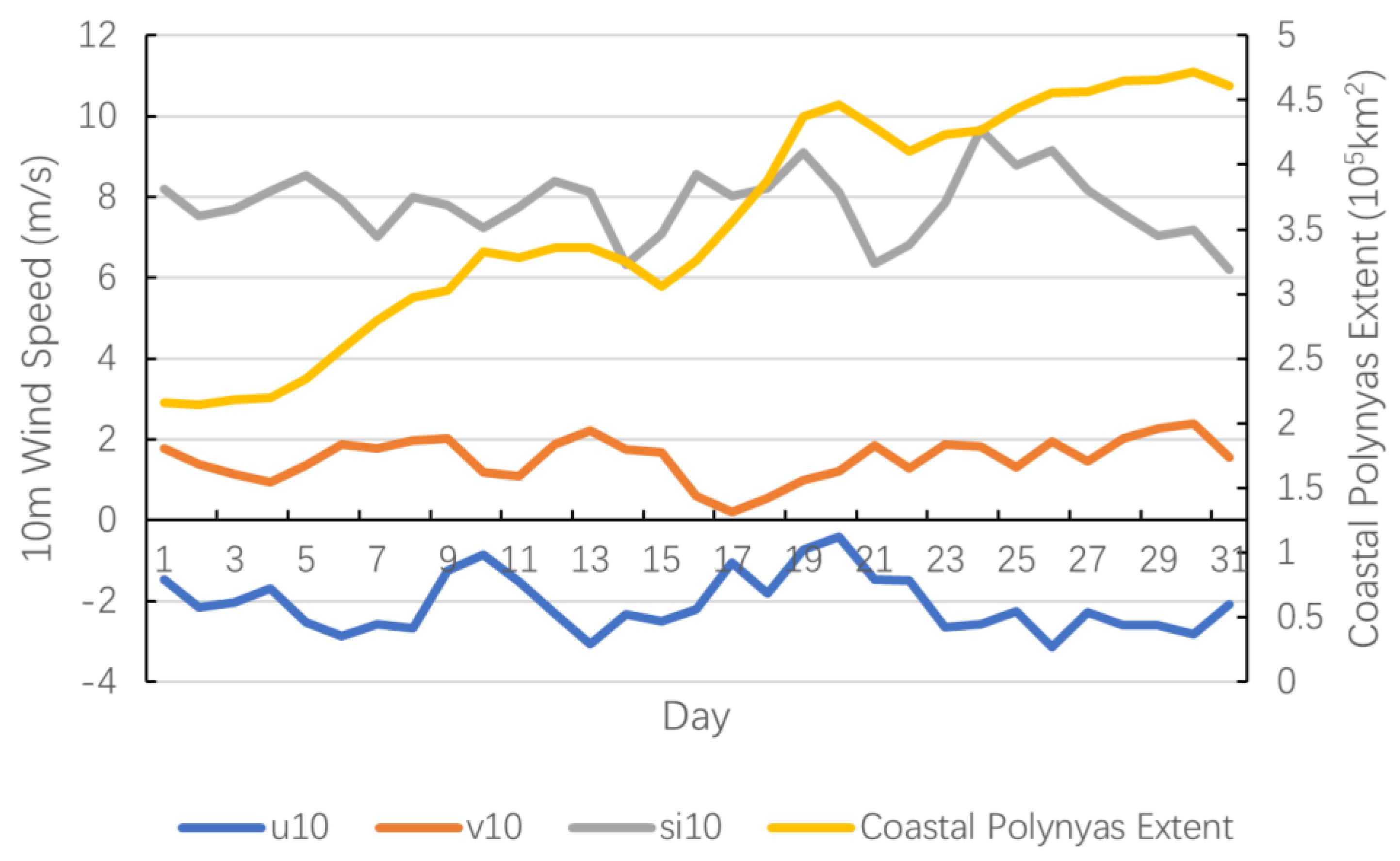
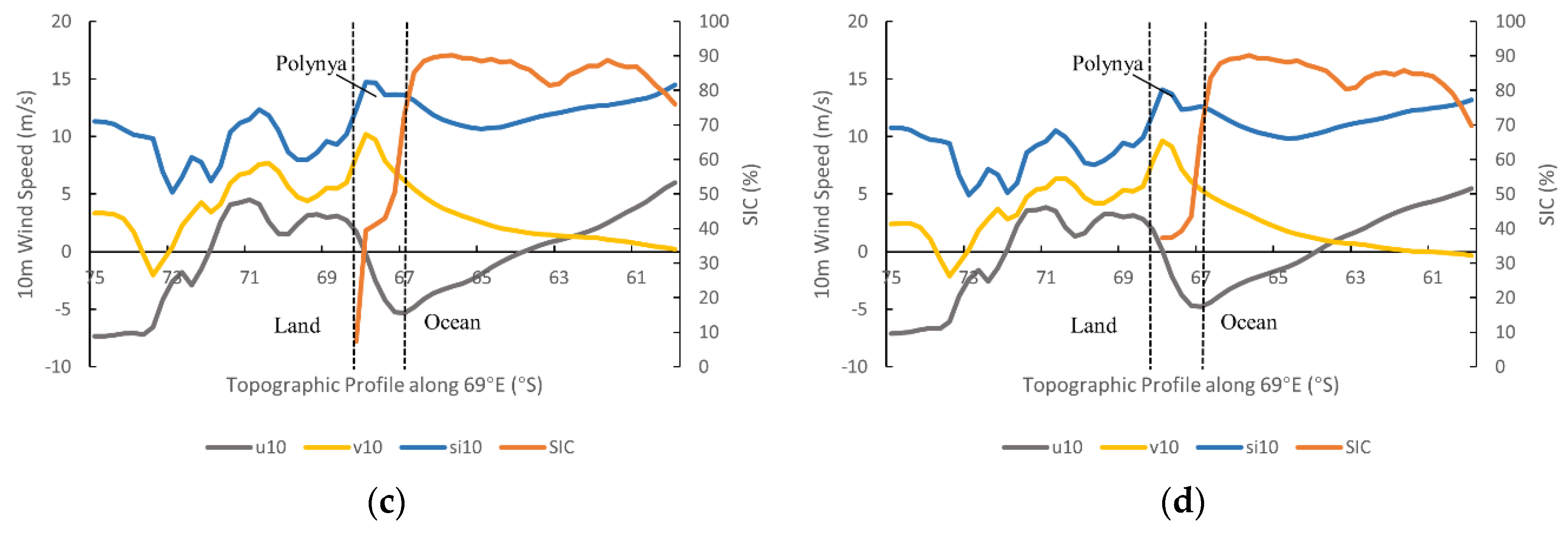
3.2.2. The Relationship Between Coastal Polynyas and Wind

Surfaces winds directly affect the formation and distribution of polynyas at coastal locations along the Southern Ocean [34]. The horizontal and vertical distribution of wind are important factors for studying the stability of coastal polynyas. Three types of wind variables were selected to analyze the impact on coastal polynyas. Taking October 2018 as an example, the 24-h data of the three wind variables in a day were averaged to represent the average wind speed on that day. The distribution of coastal polynyas was compared with the three daily averaged wind speed variables of the region in October 2018 in Figure 11. The coastal polynyas extent was extracted with the original SIC products in October 2018.
It can be seen from Figure 11 that the line of coastal polynyas extent is the process growing as a whole in October 2018. The wind speeds of the si10 variable fluctuated more in the second half of October than in the first half of the month, and the coastal polynyas extent increased more in the second half of the month than in the first half of the month. There is little difference between the wind speed of the u10 component and v10 component in 10 m, and the fluctuation of the u10 component is slightly higher than the v10 component. There is a phenomenon of a slightly symmetrical distribution between the two. In general, when the u10 component wind speed decreases, the v10 component increases, and vice versa. No obvious pattern was found between the two and the coastal polynyas extent.
According to the positions of the six meridians in Figure 9a, the three variables of wind speed and coastal polynyas were analyzed by cross section. Firstly, three variables of the 24-h wind speeds from October 20 1992 to 2018 were selected, and then the daily data were averaged. Finally, the annual average wind speed of the three variables was obtained by averaging the data on October 20 each year. Figure 12 shows the wind speed and SIC profiles on the six meridians.
It can be seen from Figure 12 that at the edge of the coast and land, the variation trend of the si10 wind speed in most areas is generally consistent with the v10 component, and just opposite to the u10 component. The wind speed of the v10 component remains constant or decreases slightly while the increase of the u10 component causes the si10 speed to increase at the depth of the ocean. Most sections experienced a process of the wind speed decreasing first and then increasing sharply near the location of the coastal polynyas. Additionally, this wind speed change location is also the location where the bed elevation changes abruptly in most areas.
To study the effect of seasonal temporal changes in wind speed on polynyas, days at the four times in late winter and early spring were analyzed on October 13, 18, 23, and 28, respectively. The wind speeds of these four days were averaged from 1992 to 2018. Section (c) passes through a clear polynya along 69°E, and its change at the four days is shown in Figure 13 as an example.
As can be seen from Figure 13a–d, the three variables of wind speed as a whole have a consistent trend. The wind speeds of si10 and v10 show signs of decline from Figure 13a–d, especially in the location of the coastal polynya. There are signs of sea ice melting at the coastal polynya, especially the thin ice near the land, which even melts into the sea water.

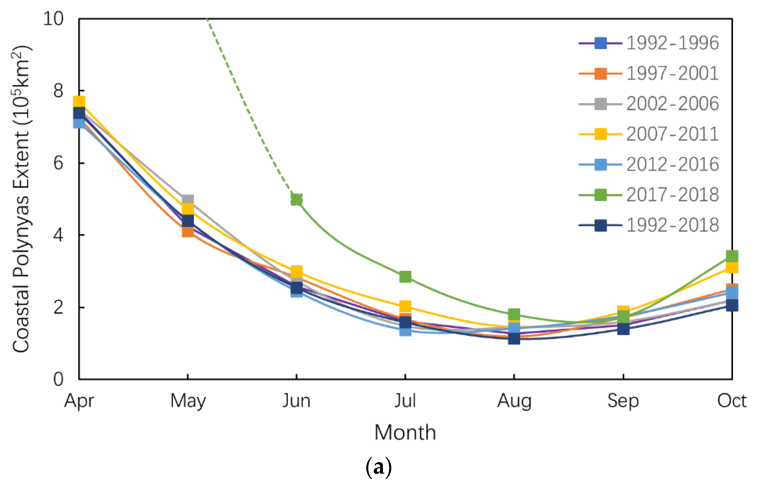
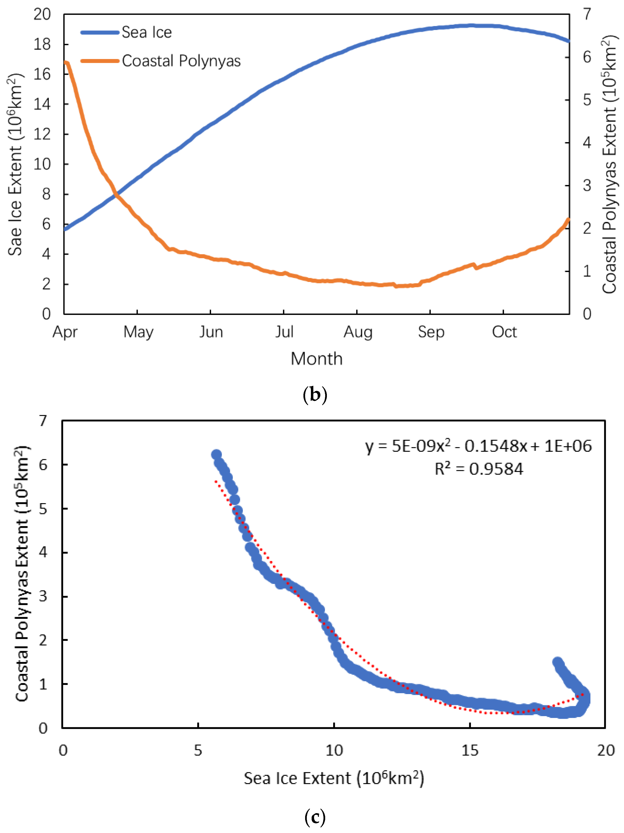
3.3. Stability Changes of Coastal Polynyas

Due to the seasonal appearance of the Southern Ocean coastal polynyas, this study chose the sea ice and coastal polynyas for a stability analysis covering the 214 days (from April to October) of the glaciated period. The 214-day SIC product, with dynamic factors removed by the spatial-temporal smoothing strategy, can objectively reflect the overall changes in polynyas over a period of years. Additionally, the threshold segmentation method was used to extract sea ice and coastal polynya regions from the spatially smoothed SIC data. This paper indicated the coastal polynyas in general are stable and analyzed the relationship with the sea ice extent of the Southern Ocean in Figure 14. In order to study the changes in polynyas over the past 27 years, this paper calculated the extent of the coastal polynyas from the spatially smoothed data for five-year periods (1992–1996, 1997–2001, 2002–2006, 2007–2011, 2012–2016), the past two years (2017–2018), and all 27 years (1992–2018) in Figure 14a. The stability of the coastal polynyas is closely related to the sea ice extent of the Southern Ocean. This study calculated the extent of the sea ice in the Southern Ocean and coastal polynyas (Figure 14b) and analyzed the relationship between them (Figure 14c) by using the spatially smoothed SIC data.
The changes of coastal polynyas extent in a multi-year period and its relationship with the sea ice extent of the Southern Ocean are shown in Figure 14. Figure 14a shows the extent of the coastal polynyas from the spatially smoothed SIC data for multiple years. It can be seen that the extent of coastal polynyas gradually shrinks from April to August and then gradually expands from September onwards. The sea froze later in 2017 and 2018 and the total sea ice extent was lower throughout those years, especially in 2017 (Figure 4). The extent of coastal polynyas reaches a minimum during August and is relatively stable then. While the formation of coastal polynyas in 2017 and 2018 was slower than in previous years, the minimum area of these polynyas was higher, which is in line with the sea ice extent data shown in Figure 4. To analyze whether the reduced sea ice and later formation have a significant impact on polynyas’ formation and stability, Figure 14b,c indicate the relationship between the coastal polynyas extent and sea ice extent.
Changes in sea ice throughout the Southern Ocean directly lead to changes in the extent of coastal polynyas. The statistics of the extent of sea ice and coastal polynyas are shown in Figure 14b. As the sea ice area increases, the area of coastal polynyas gradually decreases. The largest extent of sea ice occurs in August and September while the coastal polynyas cover the smallest extent in July and August. The extent of coastal polynyas decreases to a minimum one month later than the sea ice reaches its maximum. This is probably because the polynyas occur close to the Antarctic continent, and are easily affected by the temperature of the land. The Antarctic continent heats up quickly because of its low heat capacity while the heat capacity of the ocean leads to a slower temperature rise. This causes the sea ice to melt about a month later [9]. In addition, when winter begins (April–May), the waters near the coast gradually freeze, and the polynyas extent drops rapidly. From June to August, the sea ice extent continues to expand while the extent of the polynyas remains basically unchanged. As the sea ice begins to melt in October, the polynyas extent grows rapidly. Therefore, after a certain point, the polynyas extent will not continue to decrease as the sea ice expands and, once the sea ice begins to melt, the extent of the polynyas will increase rapidly.
In order to further analyze the relationship between the extent of coastal polynyas and Southern Ocean sea ice, this paper made a scatter plot analysis between them in Figure 14c. The coefficient of determination, R2, is 0.9584, showing that the sea ice and the coastal polynyas have a certain negative correlation. The fact that the coastal polynyas and sea ice do not always decrease or expand due to seasonal factors is an important factor affecting the determination coefficient. In summary, the extent of coastal polynyas is to some extent negatively correlated with the total extent of sea ice in the Southern Ocean.

4. Discussion

To analyze the annual trends in sea ice and polynyas, it is necessary to remove the influence of dynamic factors. It is easy to ignore some details that are on the edge of the thin ice area when we indicate the condition of the changing polynyas through the mean value of a period of time. With the long term time-series of SIC products and spatial smoothing algorithms, abnormal fluctuations caused by interference factors are effectively removed. This method can fully retain the detailed information of the image, which is conducive to a more accurate analysis of the stability of coastal polynyas.
The factors that have long been acting on the changes of polynyas include topography, wind, and ocean circulation. The outer edge of the area of low coastal ice concentration in the Southern Ocean has a high degree of coincidence with the edge of the local seabed topographic threshold. However, the coastal polynyas appear mostly near the seabed topographic threshold, which indicates that the topography factors are likely to be the fundamental factors leading to the formation of the polynyas. Wind is a direct factor affecting the formation and maintenance of polynyas, especially the Katabatic wind, which is an iconic climatic feature of Antarctica [54]. In the area where the land surface slope changes abruptly, the wind speed often changes rapidly, and the wind can descend towards the surface and ascend from the surface, changing the dynamic forcing on surface water and ice. Therefore, the combined effect of topographic and wind factors is likely to be the key reason for the formation and maintenance of coastal polynyas in the Southern Ocean.
Polynyas is a sensitive reactor for climate change. According to the multi-year changes in the coastal polynyas of the Southern Ocean, the formation of polynyas in 2017 and 2018 was later than in previous years, and they disappeared earlier than in previous years. The shortening of the existence period of coastal polynyas may be a sign of Antarctic climate warming.

5. Conclusions

This study used long term time-series of SIC products covering the Southern Ocean to analyze the relationship between the formation and persistence of polynyas and topographical factors. In this study, an effective method based on a spatial-temporal smoothing strategy to obtain 365-day, annual SIC products that had dynamic factors removed and which was based on SIC monitoring products was proposed for many years. This paper found a halo located on the border of areas of low and high ice concentration around the Antarctic coast, and it has a strong similarity with the local seabed in outline using the spatially smoothed SIC data and seabed. According to the distance between the two curves, it was proved that the two edges had high consistency, especially in 30°W–150°E. Through the relationship between the distribution of the polynyas and the topography, it was found that the location and slope of the steep part of the local terrain greatly affected the formation and location of the polynyas. Among them, several representative coastal polynyas, which are located at 30°W–150°E, are mainly distributed in the seabed topographic threshold. Analysis of the three wind parameters revealed that at locations where the terrain changes abruptly tends to first decrease wind and then increase wind, and this location is exactly the area where the coastal polynyas appears. Based on the combination of image expansion and threshold segmentation, we calculated the extent of coastal polynyas and sea ice using the spatially smoothed SIC data during the freezing period. It showed that there is a negative correlation between them. When the sea ice extent increases, the coastal polynyas extent decreases, and the sea ice change is nearly one month later than coastal polynyas. Fitting the extent of coastal polynyas and sea ice with a second-order polynomial, the coefficient of determination R2 reaches 0.9584, which proved that the correlation is extremely high between them. Further research may focus on the intrinsic mechanisms of the topographical and wind factors affecting the polynyas and on the other factors affecting the formation and maintenance of the polynyas.
The formation and persistence of polynyas is a complex process that is influenced by many factors. This paper identified that the combination of abrupt changes in topography and wind speed are preferential locations for polynyas. It has been shown that the topography is an important factor affecting the formation and persistence of polynyas but whether it is the fundamental factor affecting their formation remains to be shown. In a future study, we will further improve the ASI algorithm to correctly identify SIC data. It was, therefore, shown that sea ice and polynyas in the Antarctic can be effectively monitored using long-term sequences of SIC products. In this paper, we used seabed data to analyze the annual smoothed polynya data that had dynamic factors removed. The most direct evidence demonstrates the impact of topography on the formation and maintenance of polynyas and provides important support for further research into the genesis of polynyas.

Author Contributions

L.J. and F.C. conceived and designed the experiments, processed the data, and wrote the manuscript; L.J. and Y.M. processed and analyzed the data; W.Y. and Y.Q. discussed the result; W.Y. and S.Z. investigated the results and revised the manuscript; Y.M. and J.L. investigated the results, revised the manuscript, and supervised this study. All authors have read and agreed to the published version of the manuscript.

Funding

This research was supported by the Strategic Priority Research Program of the Chinese Academy of Sciences, Grant No. XDA19070201; Chinese Academy of Sciences (XDA19070201), and the International Cooperation Program of the Chinese Academy of Sciences (131211KYSB20150035) and MOST funded Multi-Parameters Arctic Environmental Observations and Information Services (MARIS) (2017YFE0111700).

Acknowledgments

We greatly thank the University of Hamburg, Germany for providing the daily sea ice concentration products (icdc.cen.uni-hamburg.de/). We truly appreciate the British Antarctic Survey for providing the Bedmap2 dataset in 2013 (https://secure.antarctica.ac.uk/data/bedmap2/), and the Copernicus Climate Change Service for providing the data of ECMWF atmospheric reanalysis of the global climate (https://cds.climate.copernicus.eu/cdsapp#!/home).

Conflicts of Interest

The authors declare no conflict of interest.

References

  1. Smith, S.D.; Muench, R.D.; Pease, C.H. Polynyas and leads: An overview of physical processes and environment. J. Geophys. Res. 1990, 37, 1086. [Google Scholar] [CrossRef]
  2. Barber, D.G.; Massom, R.A. The role of sea ice in Arctic and Antarctic polynyas. Elsevier Oceanogr. 2007, 74, 1–54. [Google Scholar]
  3. Markus, T.; Kottmeier, C.; Fahrbach, E. Ice Formation in Coastal Polynyas In the Weddell Sea and Their Impact on Oceanic Salinity. In Antarctic Sea Ice: Physical Processes, Interactions and Variability; Wiley: Hoboken, NJ, USA, 2013. [Google Scholar] [CrossRef]
  4. Gordon, A.L. Southern Ocean polynya. Nat. Clim. Chang. 2014, 4, 249. [Google Scholar] [CrossRef]
  5. Hirano, D.; Fukamachi, Y.; Ohshima, K.I.; Watanabe, E.; Mahoney, A.R.; Eicken, H.; Itoh, M.; Simizu, D.; Iwamoto, K.; Jones, J.; et al. Winter Water Formation in Coastal Polynyas of the Eastern Chukchi Shelf: Pacific and Atlantic Influences. J. Geophys. Res. Ocean. 2018, 123, 5688–5705. [Google Scholar] [CrossRef]
  6. Kim, B.; Lee, S.; Kim, M.; Hahm, D.; Rhee, T.S.; Hwang, J. An Investigation of Gas Exchange and Water Circulation in the Amundsen Sea Based On Dissolved Inorganic Radiocarbon. Geophys. Res. Lett. 2018, 45, 12368–12375. [Google Scholar] [CrossRef]
  7. Knies, J.; Köseoğlu, D.; Rise, L.; Baeten, N.; Bellec, V.K.; Bøe, R.; Klug, M.; Panieri, G.; Jernas, P.E.; Belt, S.T. Nordic Seas polynyas and their role in preconditioning marine productivity during the Last Glacial Maximum. Nat. Commun. 2018, 9, 3959. [Google Scholar] [CrossRef] [PubMed]
  8. Labrousse, S.; Williams, G.; Tamura, T.; Bestley, S.; Sallée, J.-B.; Fraser, A.D.; Sumner, M.; Roquet, F.; Heerah, K.; Picard, B.; et al. Coastal polynyas: Winter oases for subadult southern elephant seals in East Antarctica. Sci. Rep. 2018, 8, 3183. [Google Scholar] [CrossRef] [PubMed] [Green Version]
  9. Ward, J.M.; Raphael, M.N. The circumpolar influence of large-scale atmospheric circulations on Antarctic coastal polynyas. In Proceedings of the AGU Fall Meeting Abstracts, Washington, DC, USA, 10–14 December 2018. [Google Scholar]
  10. Bronselaer, B.; Winton, M.; Griffies, S.M.; Hurlin, W.J.; Rodgers, K.B.; Sergienko, O.V.; Stouffer, R.J.; Russell, J.L. Change in future climate due to Antarctic meltwater. Nature 2018, 564, 53–58. [Google Scholar] [CrossRef] [PubMed]
  11. Dimento, B.P.; Mason, R.P.; Brooks, S.; Moore, S. The impact of sea ice on the air-sea exchange of mercury in the Arctic Ocean. Deep Sea Res. Part I Oceanogr. Res. Pap. 2018, 144, 28–38. [Google Scholar] [CrossRef]
  12. Arrigo, K.R.; Dijken, G.L.V. Phytoplankton dynamics within 37 Antarctic coastal polynyas. J. Geophys. Res. 2003, 108. [Google Scholar] [CrossRef]
  13. Arrigo, K.R. Sea Ice Ecosystems. Annu. Rev. Mar. Sci. 2014, 6, 439–467. [Google Scholar] [CrossRef] [PubMed]
  14. Oliver, H.; St-Laurent, P.; Sherrell, R.M.; Yager, P.L. Controls on summer phytoplankton blooms in a highly productive Antarctic coastal polynya. In Proceedings of the AGU Fall Meeting Abstracts, Washington, DC, USA, 10–14 December 2018. [Google Scholar]
  15. Yager, P.L.; St-Laurent, P.; Oliver, H.; Sherrell, R.M.; Stammerjohn, S.E.; Dinniman, M.S. High-resolution numerical ocean model illustrates how ice-sheet ocean interactions impact the biological pump of an Antarctic coastal polynya. In Proceedings of the AGU Fall Meeting Abstracts, Washington, DC, USA, 10–14 December 2018. [Google Scholar]
  16. St-Laurent, P.; Yager, P.L.; Sherrell, R.M.; Oliver, H.; Dinniman, M.S.; Stammerjohn, S.E. Modeling the Seasonal Cycle of Iron and Carbon Fluxes in the Amundsen Sea Polynya, Antarctica. J. Geophys. Res. Ocean. 2019, 124, 1544–1565. [Google Scholar] [CrossRef] [Green Version]
  17. Schauer, U.; Fahrbach, E. A dense bottom water plume in the western Barents Sea: Downstream modification and interannual variability. Deep-Sea Res. Part I Oceanogr. Res. Pap. 1999, 46, 2095–2108. [Google Scholar] [CrossRef]
  18. Williams, G.D.; Aoki, S.; Jacobs, S.S.; Rintoul, S.R.; Tamura, T.; Bindoff, N.L. Antarctic Bottom Water from the Adélie and George V Land coast, East Antarctica (140–149°E). J. Geophys. Res. Ocean. 2010, 115. [Google Scholar] [CrossRef]
  19. Williams, G.D.; Herraiz-Borreguero, L.; Roquet, F.; Tamura, T.; Ohshima, K.I.; Fukamachi, Y.; Fraser, A.D.; Gao, L.; Chen, H.; McMahon, C.R.; et al. The suppression of Antarctic bottom water formation by melting ice shelves in Prydz Bay. Nat. Commun. 2016, 7, 12577. Available online: https://0-www-nature-com.brum.beds.ac.uk/articles/ncomms12577#supplementary-information (accessed on 20 December 2019). [CrossRef]
  20. Maqueda, M.A.M.; Willmott, A.J.; Biggs, N.R.T. Polynya Dynamics: A Review of Observations and Modeling. Rev. Geophy. 2004, 42. [Google Scholar] [CrossRef] [Green Version]
  21. Paul, S.; Willmes, S.; Heinemann, G. Long-term coastal-polynya dynamics in the Southern Weddell Sea from MODIS thermal-infrared imagery. Cryosphere 2015, 9, 2027–2041. [Google Scholar] [CrossRef] [Green Version]
  22. Stroeve, J.; Jenouvrier, S. Mapping and Assessing Variability in the Antarctic Marginal Ice Zone, the Pack Ice and Coastal Polynyas. Cryosphere 2016, 10, 1823–1843. [Google Scholar] [CrossRef] [Green Version]
  23. Maykut, G.A. Energy Exchange Over Young Sea Ice in the Central Arctic. J. Geophys. Res. Ocean. 1978, 83, 3646–3658. [Google Scholar] [CrossRef]
  24. Tamura, T.; Ohshima, K.I.; Nihashi, S. Mapping of sea ice production for Antarctic coastal polynyas. Geophys. Res. Lett. 2008, 35, 284–298. [Google Scholar] [CrossRef]
  25. Grebmeier, J.M.; Cooper, L.W. Influence of the St. Lawrence Island Polynya upon the Bering Sea benthos. J. Geophys. Res. Ocean. 1995, 100, 4439–4460. [Google Scholar] [CrossRef]
  26. Labrousse, S.; Sallée, J.-B.; Fraser, A.D.; Massom, R.A.; Reid, P.; Hobbs, W.; Guinet, C.; Harcourt, R.; McMahon, C.; Authier, M.; et al. Variability in sea ice cover and climate elicit sex specific responses in an Antarctic predator. Sci. Rep. 2017, 7, 43236. Available online: https://0-www-nature-com.brum.beds.ac.uk/articles/srep43236#supplementary-information (accessed on 20 December 2019). [CrossRef] [PubMed] [Green Version]
  27. Gordon, A.L.; Comiso, J.C. Polynyas in the Southern Ocean. Sci. Am. 1988, 258, 90–97. [Google Scholar] [CrossRef]
  28. Cheon, W.G.; Cho, C.B.; Gordon, A.L.; Kim, Y.H.; Park, Y.G. The Role of Oscillating Southern Hemisphere Westerly Winds: Southern Ocean Coastal and Open-Ocean Polynyas. J. Clim. 2018, 31. [Google Scholar] [CrossRef]
  29. Gao, G.P.; Dong, Z.Q. Advances in Studies on Mechanism of the Weddell Polynya Formation. J. Ocean Univ. Qingdao 2004, 34, 001–006. [Google Scholar]
  30. Mezgec, K.; Stenni, B.; Crosta, X.; Masson-Delmotte, V.; Baroni, C.; Braida, M.; Ciardini, V.; Colizza, E.; Melis, R.; Salvatore, M.C.; et al. Holocene sea ice variability driven by wind and polynya efficiency in the Ross Sea. Nat. Commun. 2017, 8, 1334. [Google Scholar] [CrossRef] [Green Version]
  31. Foster, T.D. Abyssal water mass formation off the eastern Wilkes land cost of Antarctica. Deep Sea Res. Part I Oceanogr. Res. Pap. 1995, 42, 501–522. [Google Scholar] [CrossRef]
  32. Orsi, A.H.; Wiederwohl, C.L. A recount of Ross Sea waters. Deep-Sea Res. Part II: Top. Stud. Oceanogr. 2009, 56, 778–795. [Google Scholar] [CrossRef]
  33. Nihashi, S.; Ohshima, K.I. Circumpolar Mapping of Antarctic Coastal Polynyas and Landfast Sea Ice: Relationship and Variability. JCLI 2015, 28, 3650–3670. [Google Scholar] [CrossRef]
  34. Parish, T.R. Surface winds over the Antarctic continent: A review. Rev. Geophy. 1988, 26, 169–180. [Google Scholar] [CrossRef]
  35. Massom, R.A.; Harris, P.T.; Michael, K.J.; Potter, M. The distribution and formative processes of latent-heat polynyas in East Antarctica. Ann. Glaciol. 2017, 27, 420–426. [Google Scholar] [CrossRef] [Green Version]
  36. Gordon, A.L. Deep Antarctic Convection West of Maud Rise. J. Phys. Oceanogr. 2010, 8, 600–612. [Google Scholar] [CrossRef] [Green Version]
  37. Alverson, K.D. Topographic preconditioning of open ocean deep convection. J. Phys. Oceanogr. 1995, 26, 2196–2213. [Google Scholar] [CrossRef] [Green Version]
  38. Nnamchi, H.C.; Li, J.; Kucharski, F.; Kang, I.S.; Keenlyside, N.S.; Ping, C.; Farneti, R. Thermodynamic controls of the Atlantic Niño. Nat. Commun. 2015, 6, 8895. [Google Scholar] [CrossRef] [PubMed] [Green Version]
  39. Oueslati, B.; Yiou, P.; Jézéquel, A. Revisiting the dynamic and thermodynamic processes driving the record-breaking January 2014 precipitation in the southern UK. Sci. Rep. 2019, 9, 2859. [Google Scholar] [CrossRef]
  40. Holland, D.M. Explaining the Weddell Polynya—A large ocean eddy shed at Maud Rise. Science 2001, 292, 1697–1700. [Google Scholar] [CrossRef]
  41. Chafik, L.; Nilsen, J.E.Ø.; Dangendorf, S.; Reverdin, G.; Frederikse, T. North Atlantic Ocean Circulation and Decadal Sea Level Change During the Altimetry Era. Sci. Rep. 2019, 9, 1041. [Google Scholar] [CrossRef] [Green Version]
  42. Markus, T.; Burns, B.A. A method to estimate subpixel-scale coastal polynyas with satellite passive microwave data. J. Geophys. Res. Ocean. 1995, 100, 4473. [Google Scholar] [CrossRef]
  43. Ohshima, K.I.; Nihashi, S.; Iwamoto, K.J.G.L. Global view of sea-ice production in polynyas and its linkage to dense/bottom water formation. Geosci. Lett. 2016, 3, 13. [Google Scholar] [CrossRef] [Green Version]
  44. Nihashi, S.; Ohshima, K.I.; Tamura, T. Sea-Ice Production in Antarctic Coastal Polynyas Estimated From AMSR2 Data and Its Validation Using AMSR-E and SSM/I-SSMIS Data. IEEE J. Sel. Top. Appl. Earth Obs. Remote Sens. 2017, 10, 3912–3922. [Google Scholar] [CrossRef] [Green Version]
  45. Preußer, A.; Ohshima, K.I.; Iwamoto, K.; Willmes, S.; Oceans, G.H. Retrieval of wintertime sea-ice production in Arctic polynyas using thermal infrared and passive microwave remote sensing data. JGR Oceans 2019, 124, 5503–5528. [Google Scholar] [CrossRef] [Green Version]
  46. Zhao, J.; Zhou, X.; Sun, X.; Cheng, J.; Bo, H.U.; Chunhua, L.I.; Press, C.O. The inter comparison and assessment of satellite sea-ice concentration datasets from the arctic. J. Remote Sens. 2017. [Google Scholar] [CrossRef]
  47. Comiso, J.C.; Meier, W.; Markus, T. Annomalies and Trends in the Sea Ice Cover from 40 years of Passive Microwave Data. In Proceedings of the AGU Fall Meeting Abstracts, Washington, DC, USA, 10–14 December 2018. [Google Scholar]
  48. Kaleschke, L.; Lüpkes, C.; Vihma, T.; Haarpaintner, J.; Bochert, A.; Hartmann, J.; Heygster, G. SSM/I Sea Ice Remote Sensing for Mesoscale Ocean-Atmosphere Interaction Analysis. J. Remote Sens. 2001, 27, 526–537. [Google Scholar] [CrossRef]
  49. Spreen, G.K.L.; Heygster, G. Sea ice remote sensing using AMSR-E 89-GHz channels. J. Geophys. Res. 2008, 113. [Google Scholar] [CrossRef] [Green Version]
  50. Fretwell, P.; Pritchard, H.D.; Vaughan, D.G.; Bamber, J.L.; Barrand, N.E.; Bell, R.; Bianchi, C.; Bingham, R.G.; Blankenship, D.D.; Casassa, G.; et al. Bedmap2: Improved ice bed, surface and thickness datasets for Antarctica. Cryosphere 2013, 7, 375–393. [Google Scholar] [CrossRef] [Green Version]
  51. Hersbach, H.; Bell, W.; Berrisford, P.; Horányi, A.J.M.-S.; Nicolas, J.; Radu, R.; Schepers, D.; Simmons, A.; Soci, C. Global reanalysis: Goodbye ERA-Interim, hello ERA5. ECMWF Newsl. 2019, 159, 17–24. [Google Scholar]
  52. Lindsay, R.W. Halo of low ice concentration observed over the Maud Rise seamount. Geophys. Res. Lett. 2004, 31, L13302. [Google Scholar] [CrossRef] [Green Version]
  53. Pease, C.H. The Size of Wind-Driven Coastal Polynyas. J. Geophys. Res. Ocean. 1987, 92, 7049–7059. [Google Scholar] [CrossRef]
  54. Barthélemy, A.; Goosse, H.; Mathiot, P.; Fichefet, T. Inclusion of a katabatic wind correction in a coarse-resolution global coupled climate model. Ocean Model. 2012, 48, 1203. [Google Scholar] [CrossRef]
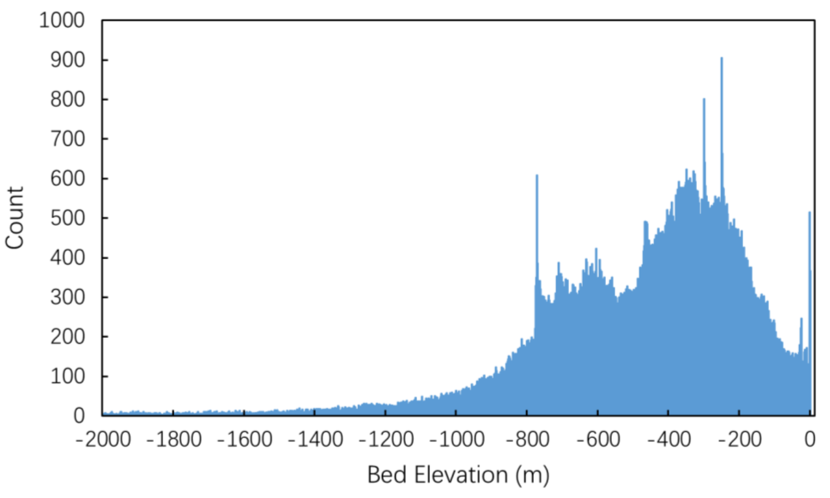
Figure 1. The spatial multi-smoothing algorithm flow chart.
Remotesensing 12 01043 g001
Figure 2. The detailed flow chart of the spatial multi-smoothing algorithm (taking data processing from 1992 to 2018 as an example).
Remotesensing 12 01043 g002
Figure 3. Comparison of the spatial smoothing and the pixel-based averaging results on October 20. (a) represents the final annual data on October 20 that have been spatially smoothed using 27-year SIC products, and (b) shows the result based on the average of pixel values of SIC data on October 20 in 27 years, which is provided for comparison. (c) is an enlarged image of the blue rectangular area of (a), and (d) is an enlarged image of (b) at the same position within the frame.
Remotesensing 12 01043 g003aRemotesensing 12 01043 g003b
Figure 4. Comparison of the sea ice extent over 365-day periods. The black dotted line represents the sea ice extent obtained by applying the spatial smoothing algorithm to data from 1992–2018; the blue dotted line represents the sea ice extent obtained using the pixel-by-pixel means. The sea ice extent from the original data for 1992, 1997, 2002, 2007, 2012, 2017, and 2018 was used as a reference.
Remotesensing 12 01043 g004
Figure 5. Comparisons of the percentage of SIC for one pixel point obtained using the method of spatially smoothed and pixel-based averaging. The orange line represents the sea ice area obtained using the spatial smoothing algorithm. The blue line represents the sea ice area obtained using the pixel-by-pixel mean.
Remotesensing 12 01043 g005
Figure 6. Analysis of the extracted outer edge of the area of low coastal ice concentration and the edge of the seabed topographic threshold. (a,b) show the extraction results for the outer edge of the region of low coastal ice concentration and the edge where the abrupt change in the seabed occurs. The results were obtained using a processed SIC product as the base map (a) and the seabed elevation from Bedmap2 as the base map (b). The yellow line represents the outer edge of the area of low ice concentration, and the red line represents the line where the seabed drops steeply. (c) is an enlarged image of the blue rectangular area of (a).
Remotesensing 12 01043 g006
Figure 7. Distance analysis for the two edges. The abscissa is the sampling point and the ordinate is the distance after the Z-score normalization process. The small image in Figure 7 shows the distance analysis for Maud Rise.
Remotesensing 12 01043 g007
Figure 8. Distribution of polynyas against the bed elevation. Values of bed elevation less than −2000 m are ignored.
Remotesensing 12 01043 g008
Figure 9. Distribution of coastal polynyas on slope and winds. (a) shows the distribution of coastal polynyas on slope. The six red lines (a–f) represent the locations of the six meridional sections, which are located at 3°E, 12°E, 69°E, 110°E, 145°E, and 112°W, respectively. (b) shows the distribution of coastal polynyas on winds.
Remotesensing 12 01043 g009
Figure 10. Topographic profile map. (af) show the profiles for the six meridional sections passing through polynyas or the Maud Rise in Figure 9a. Of these, section (a) passes through the Maud Rise, the polynyas in (b) and (c) are located where the local topography abruptly changes, and the polynyas in (d) and (e) occur before the local topography drops rapidly. The polynya in (f) appears well before this rapid change occurs. In each case, the locations of the Antarctic continent, polynyas, and ocean are shown.
Remotesensing 12 01043 g010
Figure 11. Distribution of coastal polynyas and three wind variables.
Remotesensing 12 01043 g011
Figure 12. Wind profile map. The position of each subfigure corresponds to each meridian of Figure 9.
Remotesensing 12 01043 g012aRemotesensing 12 01043 g012b
Figure 13. Wind profile map of section (c). Subfigure (ad) represent maps on October 13, 18, 23, and 28, respectively.
Remotesensing 12 01043 g013aRemotesensing 12 01043 g013b
Figure 14. Extent statistics and analysis of coastal polynyas. (a) The extent of the coastal polynyas was extracted from the spatially smoothed SIC data for April to October 1992–1996, 1997–2001, 2002–2006, 2007–2011, 2012–2016, 2017–2018, and 1992–2018. (b) Extent statistics for sea ice and coastal polynyas. The sea ice and coastal polynya areas for April to October were extracted from the spatially smoothed SIC data of the Southern Ocean. (c) Scatter plot of coastal polynyas extent against sea ice extent. A second-order polynomial was used to fit the 214-day sea ice and coastal polynya data from the spatially smoothed SIC data of the Southern Ocean.
Remotesensing 12 01043 g014aRemotesensing 12 01043 g014b
Table 1. Table showing statistics related to the distribution of polynyas.
Bed Elevation (m)Area (km2)Percentage (%)Accumulated Percentage (%)
<−200014230.450.45
−2000 ~ −18008870.280.73
−1800 ~ −160011110.351.08
−1600 ~ −140016690.521.60
−1400 ~ −120035481.112.71
−1200 ~ −100068872.164.87
−1000 ~ −80020,1566.3211.19
−800 ~ −60059,76918.7429.93
−600 ~ −40071,41122.4052.33
−400 ~ −200104,83832.8885.21
−200 ~ 047,17414.79100
Total318,873100100

