Partitioned Relief-F Method for Dimensionality Reduction of Hyperspectral Images

Abstract

The classification of hyperspectral remote sensing images is difficult due to the curse of dimensionality. Therefore, it is necessary to find an effective way to reduce the dimensions of such images. The Relief-F method has been introduced for supervising dimensionality reduction, but the band subset obtained by this method has a large number of continuous bands, resulting in a reduction in the classification accuracy. In this paper, an improved method—called Partitioned Relief-F—is presented to mitigate the influence of continuous bands on classification accuracy while retaining important information. Firstly, the importance scores of each band are obtained using the original Relief-F method. Secondly, the whole band interval is divided in an orderly manner, using a partitioning strategy according to the correlation between the bands. Finally, the band with the highest importance score is selected in each sub-interval. To verify the effectiveness of the proposed Partitioned Relief-F method, a classification experiment is performed on three publicly available data sets. The dimensionality reduction methods Principal Component Analysis (PCA) and original Relief-F are selected for comparison. Furthermore, K-Means and Balanced Iterative Reducing and Clustering Using Hierarchies (BIRCH) are selected for comparison in terms of partitioning strategy. This paper mainly measures the effectiveness of each method indirectly, using the overall accuracy of the final classification. The experimental results indicate that the addition of the proposed partitioning strategy increases the overall accuracy of the three data sets by 1.55%, 3.14%, and 0.83%, respectively. In general, the proposed Partitioned Relief-F method can achieve significantly superior dimensionality reduction effects.

1. Introduction

With the development of remote sensing and spectral imaging technologies, the amount of research into hyperspectral images (HSIs) has been increasing in recent years, occupying an important position [1]. Hyperspectral sensors are capable of acquiring continuous spectra of hundreds of bands simultaneously for each pixel. Compared with multispectral images (MSIs), HSIs undoubtedly contain more detailed spectral information, providing a better resource for the recognition or classification of ground objects [2]. There are currently many hyperspectral imaging systems providing a number of hyperspectral data sets, which are often used as research objects, such as AVIRIS (USA), HYDICE (USA), HyMAP (Australia), and ROSIS (Germany) [3].

When classifiers, such as SVM, KNN, and Neural Networks, are directly used to classify HSI data, the classification accuracy is generally low; this is mainly due to the Curse of Dimensionality. As high-dimensional data contain more information, their use should lead to better results for classification tasks (or other tasks). However, with the increase of the data dimension, the computational cost of the model tends to increase exponentially and, in the case of a small number of samples, it is difficult for the model to learn useful information to improve performance; this is the meaning of the Curse of Dimensionality [4]. The Hughes phenomenon indicates that the accuracy of HSI classification will not continue to increase with the addition of new bands but, in fact, may decrease after the accuracy reaches a certain level [5]. Due to the high dimensionality of HSIs, the amount of data required for MSI classification typically does not meet the needs of HSI classification. The linear inseparability of HSIs also makes it difficult to apply traditional MSI classifiers directly to HSIs [6].

In summary, the problem of high dimensionality should be solved before classification. Dimensionality reduction methods provide an effective way to deal with this problem, which are generally divided into feature extraction and feature selection. Feature extraction refers to mapping the original high-dimensional space into a low-dimensional space by combining features according to certain rules. Common feature extraction methods for HSI dimensionality reduction include Principal Component Analysis (PCA) [7], Minimum Noise Fraction (MNF) transforms [8], Independent Component Analysis (ICA) [9], Linear Discriminant Analysis (LDA) [10], Singular Value Decomposition (SVD) [11], Wavelet Transforms (WT) [12], and other algorithms. Feature extraction preserves all original feature information but destroys the intrinsic feature structure. Feature selection refers to selecting a representative subset from the original band set as the classification basis without losing important information. HSI dimensionality reduction methods based on feature selection can be divided into supervised and unsupervised, from the perspective of whether class marking is needed. Unsupervised feature selection methods only use the information contained in the data itself to select the bands, such as Optimum Index Factor (OIF) [13], Automatic Band Selection (ABS) [14], Hierarchical Clustering [15], K-Means Clustering [16], Particle Swarm Optimization (PSO) [17], and so on. Supervised feature selection methods require the use of class marking for band selection, such as Sequential Forward Selection (SFS) [18], Sequential Forward Floating Selection (SFFS) [19], Suboptimal Search Strategy (SSS) [20], and so on. Relief-F is a supervised feature selection method used for the dimensionality reduction of HSIs [21].

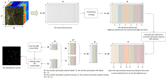
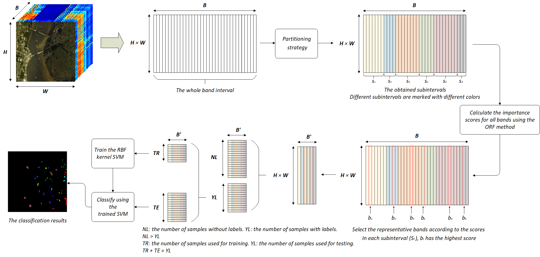
An HSI can be regarded as a data cube containing three dimensions, denoted as $X\in {\mathbb{R}}^{H\times W\times B}$, where H and W represent the two spatial dimensions of the scene, and B represents the spectral dimension. Therefore, the HSI contains $H\times W$ pixels, where each pixel contains B bands. In a supervised hyperspectral classification task, a pixel represents a sample that records the spectral information of a ground object. Generally, we need to reduce the dimensionality of the data before classification. The band selection method can be regarded as selecting the most representative $B^{\prime }$ $(B^{\prime }\ll B)$ bands to form a new, low-dimensional data cube, denoted as $X\in {\mathbb{R}}^{H\times W\times B^{\prime }}$. In band selection methods, the selected band subset is required to have rich information and low redundancy. In the original Relief-F (ORF) method, the bands are sorted according to their calculated importance scores and the top k bands are selected to form a new data set to achieve data dimensionality reduction. However, ORF can only guarantee that the information on the data is rich. According to our research, it is easy to obtain adjacent bands using ORF, but the adjacent bands may be highly correlated. Therefore, in this paper, we propose an improved Partitioned Relief-F (PRF) method for band selection of HSIs. We can reshape the three-dimensional cube into a two-dimensional matrix, $X\in {\mathbb{R}}^{N\times B}$ ($N=H\times W$), where each column is a band of the entire HSI, and all B bands can be regarded as one interval. In PRF, a partitioning strategy is proposed to divide the entire interval, in an orderly manner, to obtain multiple sub-intervals. The importance score of each band is calculated by ORF, and the band with the highest score is selected as the representative band of each sub-interval. As the partitioning strategy brings together highly correlated bands, the new low-dimensional data composed of bands selected from different sub-intervals would have lower redundancy. Additionally, as SVMs perform well on small sample data sets [22], we chose an RBF-kernel SVM as the final classifier to address the reality of the high cost of HSIs. The details of the proposed method are described in Section 3, and Figure 1 can be used as a reference for the entire model.

The remainder of this paper is organized as follows. Section 2 introduces the related work of dimensionality reduction for HSIs, including feature extraction and feature selection. Section 3 details the proposed methods. Section 4 presents the experimental results and analysis. The conclusion is given in Section 5.

2. Related Works

As HSIs contain narrow spectral bands over a continuous spectral range, adjacent bands in an HSI are usually highly correlated. Generally, HSIs have dozens or even hundreds of bands, which results in a high-dimensional data cube. The high dimensionality of the data causes considerable problems for classification tasks. Therefore, many researchers have been working on attempting to propose a reasonable and effective dimensionality reduction method for HSIs.

2.1. Feature Extraction Methods

In the dimensionality reduction of hyperspectral data, it is necessary to use some appropriate transformations as the non-linear features of HSI data cannot be extracted by using the common feature extraction methods. Non-linear features can be extracted by introducing kernel functions, through transforming the original data into a new high-dimensional space through a non-linear mapping and, then, using standard methods for low dimensional mapping [23]. For instance, the traditional PCA method can extract non-linear features from HSI data after combining kernel methods. Fauvel et al. demonstrated that the features extracted by Kernel-based Principal Component Analysis (KPCA) are more linearly separable than those extracted by the traditional PCA method [24]. Li X et al. proposed a Two-stage Subspace Projection framework, in which they used the KPCA method to carry out feature projection of HSI data [25]. Further improvement methods have been proposed on the basis of KPCA, such as Super pixelwise KPCA [26] and Multiple KPCA based on integrated learning [27].

Kernel techniques have also been combined with other feature extraction methods (except for PCA). Zhao B et al. proposed an optimized Kernel Minimum Noise Fraction (optimized KMNF) in which the noise is estimated using more stable spectral correlation information [28]. Gomez-Chova et al. proposed a KMNF method for explicitly estimating noise in a regenerative kernel Hilbert space, which is more noiseless than MNF and other KMNF methods [29]. The kernel technique also has been combined with ICA. Song S et al. verified the effectiveness of kernel ICA in the feature extraction of HSI data for anomaly detection tasks [30]. Han Z et al. conducted dimensionality reduction on feature sets based on quantitative histogram matrix (QHM) and the improved kernel ICA when using HSIs to identify qualified and adulterated petroleum products [31]. The kernel technique has also been combined with other traditional feature extraction methods. For instance, Yuan H et al. extended LDA to kernel LDA by incorporating a local scatter matrix from a small neighborhood as a regularization term into the objective function of LDA [32]. Gu Y et al. proposed an algorithm called rare signal component extraction (RSCE) for an anomaly detection task in HSIs, in which KSVD was used for feature extraction [33]. Du P et al. used the Coiflet kernel function in Wavelet Transform, which enabled the constructed wavelet SVMs to obtain high accuracy in the classification of HSIs [34].

In addition to introducing kernel functions to extract non-linear features from HSI data, there are also feature extraction methods based on manifold learning. Manifold learning uses local measurement information, which is easy to measure to learn the underlying global geometric structure of the data set, and is able to mine non-linear features [35]. Many non-linear dimensionality reduction algorithms based on manifold learning have been proposed and applied in HSI data, such as Isometric Mapping (ISOMAP), Laplacian Eigenmaps (LE), Locally-linear Embedding (LLE), Locality Preserving Projection (LPP), and so on. These non-linear dimensionality reduction methods also change correspondingly when applied to HSI data. For example, Orts Gomez et al. combined ISOMAP with SMACOF, the most accurate MDS method, to reduce the dimensionality of HSI data [36]. Zhou S et al. proposed an improved ISOMAP algorithm, which uses the neighborhood distance to indicate the manifold structure of HSI data, in order to improve the calculation rate [37]. Yan L et al. improved the LE-based dimensionality reduction method to enable the processing of missing data problems in multi-temporal HSIs [38]. Qian SE et al. proposed an improved dimensionality reduction algorithm by combining LLE with LE, which has more advantages in terminal member positioning and terminal element recognition [39]. Feng F et al. proposed a graph-based discriminant analysis method for spectral similarity to solve the problem that using the Euclidean distance in the LPP algorithm could not measure spectral variation well [40].

2.2. Feature Selection Methods

Feature selection methods select a feature subset from an HSI without losing important information by directly discarding a large number of “irrelevant” or “redundant” features. Therefore, feature selection methods mainly focus on two approaches: determining the validity of the selected bands (i.e., the selected bands should contain enough information); and eliminating the redundancy of the selected bands (i.e., the correlation between the selected bands should be low). Among current studies into band selection methods, ranking-, searching-, and clustering-based methods have received the most attention; however, methods based on sparsity theory have also become popular in recent years [41].

Ranking-based methods rank the bands by calculating the importance score of each band and, then, select a specified number of top-ranked bands as a band subset. The importance score is sometimes calculated based on a positive indicator, such as the optimal index factor (OIF), which measures the amount of information in the band [42]; and sometimes based on a negative indicator, such as recursive divergence, which measures the maximum separability between categories [43]. Some supervised dimensionality reduction methods have also been studied. For example, Mahlein et al. used the Relief-F algorithm for feature selection, which required the class signature of the sample [44]. In searching-based methods, a criterion function is defined to measure a subset of bands, and a search strategy is used to select different band subsets to optimize the defined criterion function. Du Q proposed a sequential forward search (SFS) method based on the abundance estimation of end members for feature selection and introduced a floating search strategy based on this, which further improved the classification accuracy [45]. Sun K et al. proposed a minimum noise band selection (MNBS) method based on sequential backward search (SBS) [46]. Furthermore, evolutionary calculation-based methods have also been used as search strategies. For example, Ghamisi et al. proposed a new binary optimization method based on fractional Darwin particle swarm optimization (FODPSO) to solve the dimensionality reduction problem [47]. Vaiphasa et al. demonstrated the effectiveness of genetic algorithms for band selection in HSIs [48].

Clustering-based methods give priority to the separability between bands and select the optimal band in each cluster after clustering the bands. For example, Martinez-Uso et al. used hierarchical clustering to group bands before selection with mutual information and Kullback–Leibler divergence [49]. Cao X et al. proposed an automatic band selection (ABS) method, which uses the KODAMA algorithm to cluster before selecting the optimal band with the minimum average Euclidean distance in each class [14]. Imbiriba T et al. proposed a band selection strategy based on reproducing kernel Hilbert spaces, which effectively extracts the non-linear features of HSI data, where the basic clustering method used was K-Means [50]. Sparsity-based methods, based on sparsity theory, reduce the dimension by learning a sparse representation of the original data. For example, Li S et al. used the existing K-SVD algorithm to obtain sparse representations of HSI data and selected the optimal band subset by calculating the histogram of the coefficient matrix [51]. Sun W et al. proposed a Symmetric Sparse Representation (SSR) method for band selection, based on the assumption that the selected band subset and the original data set could be sparsely represented similarly to each other [52]. After the analysis of various kinds of band selection methods, this paper presents the PRF method, which incorporates a partitioning strategy into ORF and can be regarded as a synthesis of a ranking-based method and a clustering-based method.

3. Proposed Method

As mentioned earlier, adjacent bands in an HSI are highly correlated as the hyperspectral sensor acquires data over a continuous spectral range. To verify the correlation between adjacent bands, we provide a statistical t-test in Section 3.2. The proposed model for HSIs is shown in Figure 1. After processing the data, as shown in Section 4.1, the three-dimensional HSI cube is reshaped into a two-dimensional matrix $X\in {\mathbb{R}}^{N\times B}$ ($N=H\times W$), where each column represents a band and each row records the spectra of a single pixel. As shown in Figure 1, we first use a partitioning strategy to divide the whole band interval, where different sub-intervals are marked with different colors. Then, the importance scores of all bands are calculated using the ORF method, which can also be calculated before the partition. In each sub-interval, the band with the highest score is selected as the representative band. These representative bands are used to form a new data cube of lower dimension $X\in {\mathbb{R}}^{H\times W\times B^{\prime }}$ ($B^{\prime }\ll B$). The above processes are the general flow of the Partitioned Relief-F (PRF) method. For classification purposes, some distinguishable pixels in the HSI are manually labeled, while others are not. Therefore, the unlabeled pixels need to be eliminated first. For labeled pixels, some are used for the training set to train the SVM classifier, while the rest are used as the test set, to verify the performance of the model. The division ratio of the training set is introduced in Section 4.1.

3.1. Band Importance Score Calculation

The original Relief-F (ORF) method is a typical supervised ranking-based band selection method, which selects the top k bands as the band subset according to the calculated importance score of each band. The importance score measures the selection priority of each band, which is calculated according to the similarities and dissimilarities of the bands. Based on this, we set “near-hit” and “near-miss” to calculate the required “similarity contribution” and “dissimilarity contribution”, respectively.

The training set of the given HSI data is recorded as $H^{nB}=\left\{\left(x_1,y_1\right),\left(x_2,y_2\right),\dots ,\left(x_n,y_n\right)\right\}$, where $x_i$ represents one pixel of the hyperspectral image, which is a one-dimensional vector (size is $B\times 1$); $y_i$ represents the category tag to which $x_i$ belongs; and $y_i\in \left(1,2,\dots ,m\right)$, in which the number of categories of the training set is m. In this paper, the Pearson correlation coefficient is used as a distance metric for the calculation of “near-hit” and “near-miss”:

$$corr\left(x_i,x_j\right)=\frac{Cov\left(x_i,x_j\right)}{\sqrt{Var\left(x_i\right)·Var\left(x_j\right)}},$$

(1)

where $x_i$ and $x_j$ represent two different pixel points in $H^{nB}$ (i.e., $i\ne j$); $Cov\left(x_i,x_j\right)$ is the covariance of $x_i$ and $x_j$; and $Var\left(x_i\right)$ is the variance of $x_i$. The “near-hit” is calculated in a sample set with the same class (let this sample set be K). For a pixel $x_i$ in K, its “near-hit” can be obtained by calculating the maximum correlation coefficient:

$$corr\left(x_i,x_{nh}\right)=\underset{j\ne i,x_j\in K}{max}corr\left(x_i,x_j\right).$$

(2)

On the contrary, the “near-miss” is calculated in other sample sets with different categories from $x_i$, which can be obtained by calculating the minimum correlation coefficient:

$$corr\left(x_i,x_{l,nm}\right)=\underset{x_j\in L}{min}corr\left(x_i,x_j\right),$$

(3)

where $x_{l,nm}$ represents the “near-miss” of $x_i$ in the sample set L, where L is one of the sample sets of different categories from $x_i$.

In the PRF method proposed in this paper, $a\left(a>1\right)$ samples are randomly selected as the base samples in each sample set. Thus, there are $a\times m$ base samples, assuming that the number of classes is m. We denote the base sample as $x_i$, where $i=0,1,\dots ,a\times m$, the corresponding “near-hit” is denoted as $x_{i,nh}$, and the “near-miss” is denoted as $x_{i,l,nm}$. Then, the importance score of each band (denoted as $Scor{e}_j$) is determined by the following formula:

$$Scor{e}_j=\sum _i-diff{\left(x_i^j,x_{nh}^j\right)}^2+\sum _i\sum _{l\ne k}\left(p_l\times diff{\left(x_i^j,x_{i,l,nm}^j\right)}^2\right),$$

(4)

where $diff\left(x,y\right)=|x-y|$ and $p_l$ represents the proportion of the number of samples in sample set l to the total number of samples in the training set. Equation (4) can be divided into two parts: The former part measures the aggregation contribution of the band j to “homogeneous samples”, while the latter measures the separation contribution of the band j to “heterogeneous samples”.

3.2. Correlation Test of Adjacent Bands

The importance score calculated by the method provided in Section 3.1 can be used to measure the importance (i.e., the amount of information) of a band. However, there are similar spectral measurements between two bands of an HSI if they are adjacent, which makes the importance scores of these two adjacent bands similar as well. In order to verify the correlation between adjacent bands, we provide a statistical t-test in this section.

Calculate the maximum of correlation coefficients between each band $({\mathbf{b}}_i,i=1,2,\dots ,B)$ and all other bands as

$$max\_corr\left({\mathbf{b}}_i\right)=\underset{i\ne j}{max}\left(corr\left({\mathbf{b}}_i,{\mathbf{b}}_j\right)\right),$$

(5)

and the maximum of correlation coefficients between ${\mathbf{b}}_i$ and its adjacent bands $({\mathbf{b}}_{i+1},{\mathbf{b}}_{i-1})$ as

$$neibor\_corr\left({\mathbf{b}}_i\right)=\left\{\begin{array}{c}corr\left({\mathbf{b}}_1,{\mathbf{b}}_2\right)\mathrm{if}i=1\hfill \\ corr\left({\mathbf{b}}_B,{\mathbf{b}}_{B-1}\right)\mathrm{if}i=B\hfill \\ max\left(corr\left({\mathbf{b}}_i,{\mathbf{b}}_{i+1}\right),corr\left({\mathbf{b}}_i,{\mathbf{b}}_{i-1}\right)\right)\mathrm{if}1<i<B\hfill \end{array}\right.,$$

(6)

where $corr\left(x,y\right)$ is the correlation coefficient between x and y.

Then, $max\_corr\left({\mathbf{b}}_i\right)$ and $neibor\_corr\left({\mathbf{b}}_i\right)$ are examined for any significant differences using the paired sample t-test. Let $max\_corr\left({\mathbf{b}}_i\right)$ be $X_{1i}$ and $neibor\_corr\left({\mathbf{b}}_i\right)$ be $X_{2i}$. Then, test whether the differences ($D_i=X_{1i}-X_{2i}(i=1,2,\dots ,B)$) are significantly smaller or not. Define the null hypothesis as $H_0$: there is no difference between $max\_corr\left({\mathbf{b}}_i\right)$ and $neibor\_corr\left({\mathbf{b}}_i\right)$; that is, ${\mu }_D=0$, where ${\mu }_D$ is the mean of the differences ${\mu }_D=\sum D_i/B$. Define the alternative hypothesis as $H_1$: there is a significant difference between $max\_corr\left({\mathbf{b}}_i\right)$ and $neibor\_corr\left({\mathbf{b}}_i\right)$; that is, ${\mu }_D\ne 0$.

The t distribution statistic is as follows:

$$t=\frac{{\mu }_D-D^{\prime }}{S_D/\sqrt{B}},$$

(7)

$$S_D=\sqrt{\frac{\sum {\left(D_i-{\mu }_D\right)}^2}{B-1}}.$$

(8)

where $D^{\prime }$ is the assumed sample difference, B is the number of sample differences (here, equal to the number of bands), ${\mu }_D$ is the mean of the differences, and $S_D$ is the standard deviation of the sample difference.

3.3. Partitioning Strategy

When using the ORF method to select bands in an HSI, the “important bands” are directly selected according to the calculated importance scores to form a new data cube. In the original data set, each band can be assigned an index in spectral order: $[1,2,\dots ,B]$, where B is equal to the spectral dimension of the data set. When two bands have similar indices, the information they contain is also similar, which means that the importance scores of the two bands are likely to be similar as well. Therefore, the indices of the bands selected by the ORF method should be continuously arranged. We verified this experimentally; the results are given in Section 4.2. In addition, using the t-test provided in Section 3.2, we confirmed that there is a high correlation between adjacent bands; these results are also given in Section 4.2.

Define the band interval $[{\mathbf{b}}_1,{\mathbf{b}}_2,\dots ,{\mathbf{b}}_B]$, where ${\mathbf{b}}_i$ is an N-dimensional real vector containing the measured values of all N pixels of the HSI in the $i^{\mathrm{th}}$ band. Dividing the band interval according to the correlation between the bands can obtain multiple sub-intervals, as shown in Figure 1. In each sub-interval, a band with the highest importance score is obtained as the representative band and all the representative bands are used to form a new data set. Under proper division, the correlation between these representative bands should be low; that is, the new data set should have lower redundancy.

For a sub-interval containing m bands, the redundancy of the sub-interval is calculated, in the proposed partitioning strategy, by:

$$r=\frac{1}{m}\sum _{i=0}^{m-1}corr\left({\mathbf{b}}_i,\mathbf{c}\right),$$

(9)

where $corr(·,·)$ is used to calculate the correlation coefficient between two vectors (as shown in Equation (1)) and $\mathbf{c}$ is the “maximum average correlation vector” in the sub-interval; that is, the mean value of the correlation coefficient between the band vectors ${\mathbf{b}}_i,(i=1,2,\dots ,m)$ and $\mathbf{c}$ is the theoretical maximum,

$$\mathbf{c}=\underset{\mathbf{z}}{argmax}\frac{1}{m}\sum _{i=1}^{m}corr\left({\mathbf{b}}_i,\mathbf{z}\right).$$

(10)

Therefore, the larger the value of r, the higher the degree of aggregation between all bands in the sub-interval. As the degree of aggregation is characterized by the correlation coefficient, the value of r can be used to measure the redundancy of the sub-interval. The solution for $\mathbf{c}$ is shown below.

Assuming the average correlation coefficient between vector $\mathbf{z}$ and other band vectors is $f\left(\mathbf{z}\right)$; that is,

$$f\left(\mathbf{z}\right)=\frac{1}{m}\sum _{i=1}^{m}corr\left({\mathbf{b}}_i,\mathbf{z}\right).$$

(11)

According to Equation (1),

$$f\left(\mathbf{z}\right)=\frac{1}{m}\sum _{i=1}^m\frac{Cov\left({\mathbf{b}}_i,\mathbf{z}\right)}{\sqrt{Var\left({\mathbf{b}}_i\right)}·\sqrt{Var\left(\mathbf{z}\right)}},$$

(12)

$$f\left(\mathbf{z}\right)=\frac{1}{m}\sum _{i=1}^m\frac{Cov\left(\frac{{\mathbf{b}}_i}{\sqrt{Var\left({\mathbf{b}}_i\right)}},\mathbf{z}\right)}{\sqrt{Var\left(\mathbf{z}\right)}},$$

(13)

$$f\left(\mathbf{z}\right)=\frac{1}{m}\frac{Cov\left({\sum }_{i=1}^m\frac{{\mathbf{b}}_i}{\sqrt{Var\left({\mathbf{b}}_i\right)}},\mathbf{z}\right)}{\sqrt{Var\left(\mathbf{z}\right)}},$$

(14)

$$f\left(\mathbf{z}\right)=\frac{1}{m}\sqrt{Var\left(\sum _{i=1}^m\frac{{\mathbf{b}}_i}{\sqrt{Var\left({\mathbf{b}}_i\right)}}\right)}·\frac{Cov\left({\sum }_{i=1}^m\frac{{\mathbf{b}}_i}{\sqrt{Var\left({\mathbf{b}}_i\right)}},\mathbf{z}\right)}{\sqrt{Var\left({\sum }_{i=1}^m\frac{{\mathbf{b}}_i}{\sqrt{Var\left({\mathbf{b}}_i\right)}}\right)}·\sqrt{Var\left(\mathbf{z}\right)}},$$

(15)

$$f\left(\mathbf{z}\right)=\frac{1}{m}\sqrt{Var\left(\sum _{i=1}^m\frac{{\mathbf{b}}_i}{\sqrt{Var\left({\mathbf{b}}_i\right)}}\right)}·corr\left(\sum _{i=1}^m\frac{{\mathbf{b}}_i}{\sqrt{Var\left({\mathbf{b}}_i\right)}},\mathbf{z}\right).$$

(16)

In Equation (16), $corr\left({\sum }_{i=1}^m\frac{{\mathbf{b}}_i}{\sqrt{Var\left({\mathbf{b}}_i\right)}},\mathbf{z}\right)=1$ when $\mathbf{z}=k·{\sum }_{i=1}^m\frac{{\mathbf{b}}_i}{\sqrt{Var\left({\mathbf{b}}_i\right)}}(k\ne 0)$ and, at this time, $f\left(\mathbf{z}\right)$ attains its maximum value. Therefore, the redundancy of the sub-interval can also be calculated by:

$$max\left(f\left(\mathbf{z}\right)\right)=\frac{1}{m}\sqrt{Var\left(\sum _{i=1}^m\frac{{\mathbf{b}}_i}{\sqrt{Var\left({\mathbf{b}}_i\right)}}\right)}.$$

(17)

For the band interval $[{\mathbf{b}}_1,{\mathbf{b}}_2,\dots ,{\mathbf{b}}_B]$ in the proposed partitioning strategy, the sub-intervals are continuously divided. Therefore, the initial state of the first sub-interval (denoted as $I_1$) is $\left\{{\mathbf{b}}_1\right\}$. Calculate the redundancy of $I_1$ (denoted by r) according to Equation (17); if r is greater than the threshold (denoted by $\lambda$), add the next band ${\mathbf{b}}_2$ to $I_1$. If $r\le \lambda$, the interval division of $I_1$ is ended and the next sub-interval division is started. Therefore, the general steps of the partitioning strategy can be described as:

Step (1) Initialize the sub-interval $I_k=\left\{{\mathbf{b}}_j\right\}$, where the band ${\mathbf{b}}_{j-1}$ belongs to the previous sub-interval $I_{k-1}$.

Step (2) Add the next band ${\mathbf{b}}_{j+1}$ to the sub-interval $I_k$ and calculate the redundancy r of $I_k$. If $r>\lambda$, the band ${\mathbf{b}}_{j+1}$ will be retained in $I_k$; if $r\le \lambda$, the band ${\mathbf{b}}_{j+1}$ will be removed from $I_k$ and the next sub-interval $I_{k+1}$ will start dividing.

Step (3) Repeat Step 2 until the last band ${\mathbf{b}}_B$ is divided.

As the correlations between the bands are not the same, the sizes of the sub-intervals are also different. According to the algorithm pseudocode (Algorithm 1) of the partitioning strategy, it can be shown that, when the threshold $\lambda$ is set to a large value, the degree of redundancy in the sub-interval will also be high. At this time, the number of bands contained in the sub-interval will be smaller and, accordingly, there will eventually be many sub-intervals. Conversely, when $\lambda$ is small, there will eventually be few sub-intervals. An appropriate value for $\lambda$ was determined based on the experimental results, as detailed below.

Algorithm 1: Partitioning strategy of the Partitioned Relief-F method.

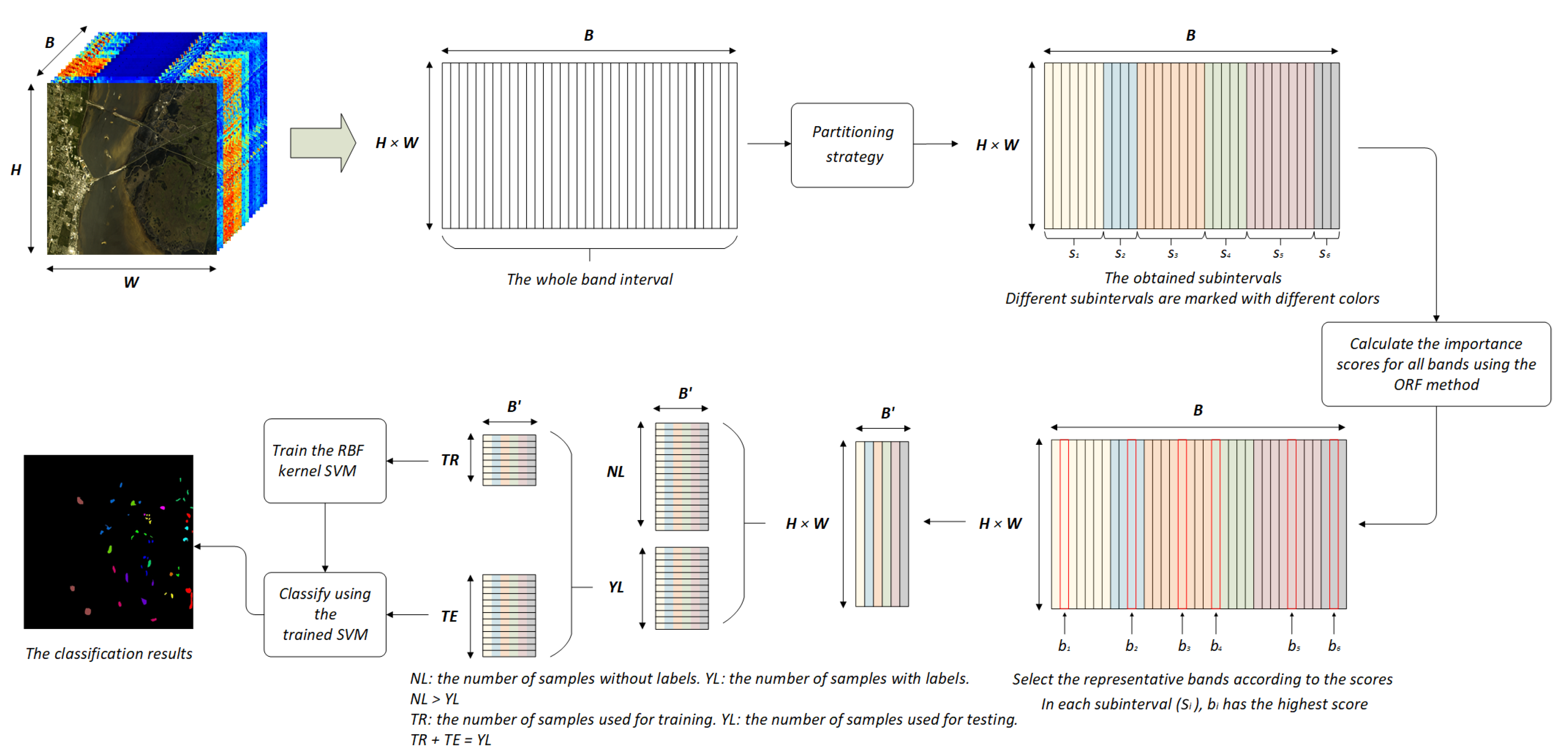
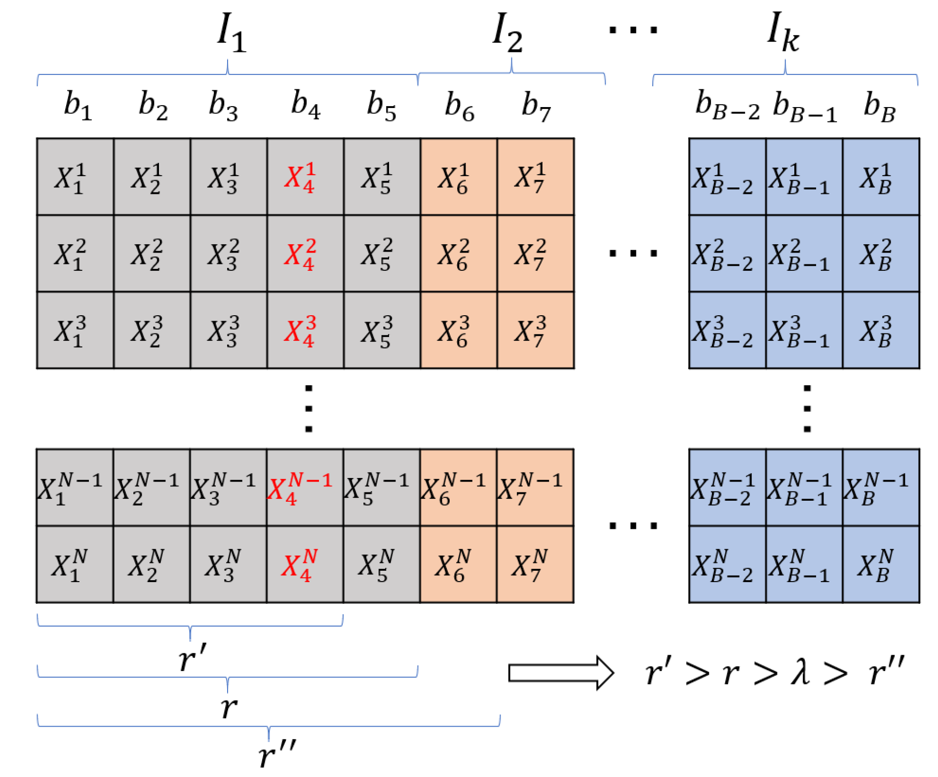
The graphical interpretation of the proposed partitioning strategy is shown in Figure 2. For the two-dimensional matrix $X\in {\mathbb{R}}^{N\times B}$, where each column represents a band, each row records the spectra of a single pixel, and ${\mathbf{X}}_j^i$ is the measured value of the $i^{\mathrm{th}}$ pixel in the $j^{\mathrm{th}}$ band. Assuming that the first sub-interval $I_1$ contains five bands (i.e., $I_1=\{b_1,b_2,\dots ,b_5\}$), as shown in the gray part in Figure 2. Let $r^{\prime }$ represent the redundancy of $\{b_1,b_2,\dots ,b_4\}$, r represent the redundancy of $I_1$, and $r^{″}$ represent the redundancy of $\{b_1,b_2,\dots ,b_6\}$. According to the description of the partitioning strategy, we have $r^{\prime }>r>\lambda >r^{″}$, where $\lambda$ is the pre-set threshold. Thus, $r^{\prime }>r>\lambda >r^{″}$ is actually the condition for the current sub-interval to stop dividing; when this condition is met, the division of the next sub-interval starts. For the obtained sub-interval, a representative band can be obtained according to the band importance score. Assuming that $b_4$ has the highest score in $I_1$, it will be selected as one of the representative bands used to form a new low-dimensional data set.

For comparison, this paper chooses two clustering algorithms—K-Means and Balanced Iterative Reducing and Clustering Using Hierarchies (BIRCH)—to partition the band interval. Similar to the PRF method, after using the clustering method to obtain multiple clusters, the representative band with highest importance score is selected from each cluster to form a new low-dimensional data set, which can also ensure that the new data set has low redundancy.

(1) K-Means: K-Means is a classic unsupervised clustering algorithm, which aims to divide data points into k clusters, where the data points in each cluster have the closest mean. For ${\mathbf{b}}_i\in {\mathbb{R}}^N$$(i=1,2,\dots ,B)$, it divides these B N-dimensional vectors into the clusters $C=C_1,C_2,\dots ,C_k$. The objective function of the K-Means algorithm is:

$$\underset{C}{argmin}\sum _{i=1}^k\sum _{\mathbf{b}\in C_i}{∥\mathbf{b}-{\mu }_i∥}_2,$$

(18)

where ${\mu }_i$ is the mean of the vectors in $C_i$. K-Means uses an iterative approach to obtain the clusters. First, randomly select k data points as the initial centroids. Then, for each data point, calculate its distance from each centroid and divide it into the same cluster with the centroid in which the distance is the shortest. After the division is completed, the mean of vectors in each cluster is calculated as the new centroid.

(2) BIRCH: BIRCH (Balanced Iterative Reducing and Clustering Using Hierarchies) is a hierarchical clustering algorithm suitable for large data sets. As with K-Means, BIRCH also needs to specify the number of clusters in advance. The core of the algorithm is to construct a clustering feature (CF) tree for hierarchical clustering, where CF is a triple that summarizes the information of the cluster. Assuming that cluster $C_i$ contains $B_i$ band vectors, the Clustering Feature of the cluster is defined as:

$${CF}_i=\left(B_i,{\overrightarrow{LS}}_i,{SS}_i\right),$$

(19)

where $B_i$ is the number of band vectors in the cluster, ${\overrightarrow{LS}}_i$ is the linear sum of the $B_i$ band vectors (i.e., ${\sum }_{i=1}^{Bi}\overrightarrow{b_i}$), and ${SS}_i$ is the square sum of the $B_i$ band vectors (i.e., ${\sum }_{i=1}^{Bi}{(\overrightarrow{b_l})}^2$). The specific process is detailed in [53].

4. Experimental Results and Discussion

In order to verify the performance of PRF in the HSI dimensionality reduction task, we selected three publicly available HSI data sets for experimental verification. The effectiveness was evaluated according to the classification accuracy using RBF-SVMs. To verify the effectiveness of PRF, we chose PCA and ORF as comparative dimensionality reduction methods. In addition, two clustering algorithms—K-Means and BIRCH—were selected for comparison in the partitioning strategy. Although each experiment had relatively stable results, in order to avoid accidental bias, the final result was the average of 10 experiments.

4.1. Data Sets

To examine the robustness of the proposed method, we selected three data sets collected from different scenes for our experiments.

(1) The Salinas data set was acquired by the AVIRIS sensor over Salinas Valley, California. AVIRIS acquires data in 224 bands of 10 nm width with center wavelengths from 400 to 2500 nm. Only 204 bands remained in the Salinas data set after removing bands covering the region of water absorption: [108–112, 154–167, and 224]. The Salinas data set consists of $512\times 217$ pixels with a spatial resolution of 3.7 m/pixel. The Salinas ground-truth contains 16 classes.

(2) The PaviaU data set was collected by the ROSIS sensor over several areas of the University of Pavia and consists of $610\times 610$ pixels with a spatial resolution of 1.3 m/pixel. In the PaviaU data set, a large part of the image is not used for the study; that is, many samples did not contain any available information. Thus, the size of the PaviaU data set was reduced to $610\times 340$ pixels. The PaviaU data set has 103 available bands of 6 nm width with center wavelengths from 430 to 860 nm. Its ground-truth contains nine classes.

(3) The KSC data set was collected by the AVIRIS sensor over the Kennedy Space Center (KSC), Florida. Therefore, it also has 224 bands with wavelengths ranging from 400 to 2500 nm. There are 176 bands remaining in KSC data set after the removal of water absorption bands and low SNR bands: [1–4, 102–116, 151–172, and 218–224]. The size of the data set is $512\times 614$ pixels, and the spatial resolution is 18 meters/pixel. The KSC ground-truth is divided into nine classes.

The original information on the three data sets is shown in

Table 1. The original information of the three data sets.

Data Set	Sensor	Spectral Range (nm)	Spectral Res. (nm)	Spatial Res. (m)	No. of Bands	No. of Classes	No. of Pixels
Salinas	AVIRIS	400–2500	10	3.7	204	16	512 × 217
PaviaU	ROSIS	430–860	6	1.3	103	9	610 × 340
KSC	AVIRIS	400–2500	10	18	176	13	512 × 614

. The classes of each data set and their corresponding number of samples are shown in

Table 2. Ground-truth classes of the three data sets.

Salinas		PaviaU		KSC
Class	Samples	Class	Samples	Class	Samples
Broccoli green weeds_1	2009	Asphalt	6631	Scrub	761
Broccoli green weeds_2	3726	Meadows	18,649	Willow swamp	243
Fallow	1976	Gravel	2099	Cabbage palm hammock	256
Fallow rough plow	1394	Trees	3064	Cabbage palm/oak hammock	252
Fallow smooth	2678	Painted metal sheets	1346	Slash pine	161
Stubble	3959	Bare Soil	5029	Oak/broadleaf hammock	229
Celery	3579	Bitumen	1330	Hardwood swamp	106
Grapes untrained	11,271	Self-Blocking Bricks	3682	Graminoid marsh	431
Soil vineyard develop	6203	Shadows	947	Spartina marsh	520
Corn senesced green weeds	3278			Cattail marsh	404
Lettuce romaine_4wk	1068			Salt marsh	419
Lettuce romaine_5wk	1927			Mud flats	503
Lettuce romaine_6wk	916			Water	927
Lettuce romaine_7wk	1070
Vineyard untrained	7268
Vineyard vertical trellis	1807
Total Number	54,129		42,777		5212

.

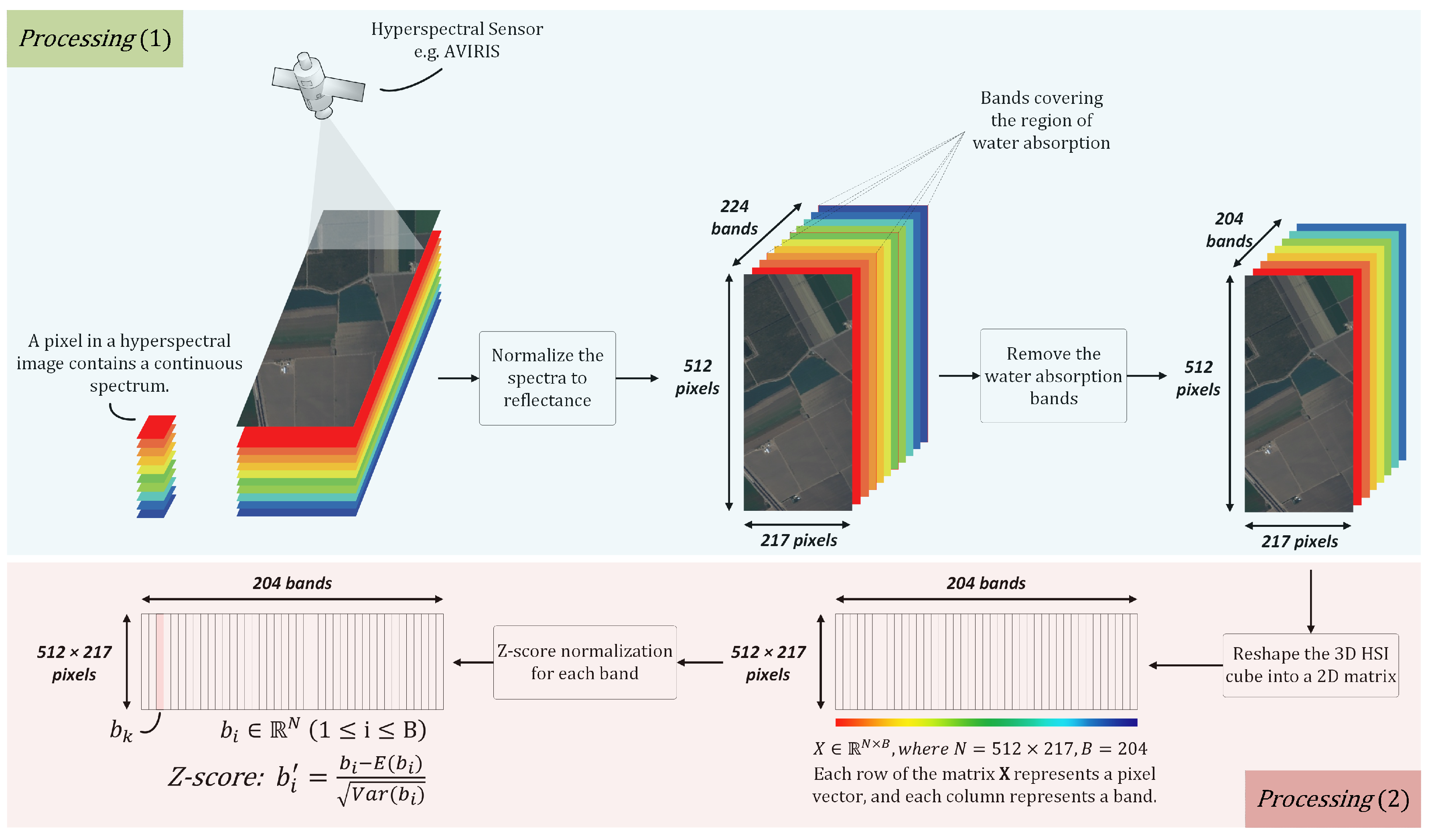
These data sets were collected by different sensors and have different spectral resolution, spatial resolution, and object classes. Therefore, we used these three data sets for experiments to obtain more comprehensive analysis results. As publicly available data sets, they have undergone some general processing; that is, the spectra have been normalized to reflectance, and the low SNR bands and water absorption bands in each data set have been eliminated, if they exist. In this paper, in order to make the classifier easy to train, the values of the HSIs were normalized to [−1, 1] using z-score normalization:

$${\mathbf{b}}_i=\frac{{\mathbf{b}}_i-E\left({\mathbf{b}}_i\right)}{\sqrt{Var\left({\mathbf{b}}_i\right)}}$$

(20)

where ${\mathbf{b}}_i\in {\mathbb{R}}^N$, ($1\le i\le B$).

To test the validity of the methods on a small sample data set, 10% of the entire HSIs were randomly selected as the training set, according to the hold-out method, in the Salinas and PaviaU data sets, and the remaining 90% of samples were used as the test set to verify the model. Considering that the sample size of the KSC data set is much smaller than the first two data sets, the proportion of the training set for the KSC data set was set at 30%.

Although the three data sets were collected from different scenes using different hyperspectral sensors, the processing done on them was similar. As shown in Figure 3, “Processing (1)” was the processing performed during the period from data collection to public access. First, the spectra of the HSI acquired by the hyperspectral sensor was normalized to reflectance. Then, the water absorption bands and/or the low SNR bands in the obtained HSI cube were eliminated. According to the information provided by the sources of the data sets, only the water absorption bands were removed in the Salinas data set, no bands were removed in the PaviaU data set, and the water absorption bands and low SNR bands were removed in the KSC data set. Figure 3 uses the Salinas data set as an example. It can be seen that, after 20 water absorption bands are eliminated, 204 bands are left in the data set. “Processing (2)” is the processing performed in this paper. First, the three-dimensional data cube is reshaped into a two-dimensional matrix, $X\in {\mathbb{R}}^{N\times B}$, where $N=512\times 217$ and $B=204$. Then, the values of each band are standardized using Equation (20), such that the bands follow the standard normal distribution. In fact, the data processing flow also includes a third stage, which is the dimensional reduction using PRF and the division of the training and test sets. This stage is shown in the model structure diagram, Figure 1.

4.2. Verification of Two Assumptions

The reason for adding the partitioning strategy to the ORF is based on two assumptions: First, a large part of the top k bands selected based on importance scores are adjacent in spectral order. Second, when two bands are adjacent, there is a high correlation between them.

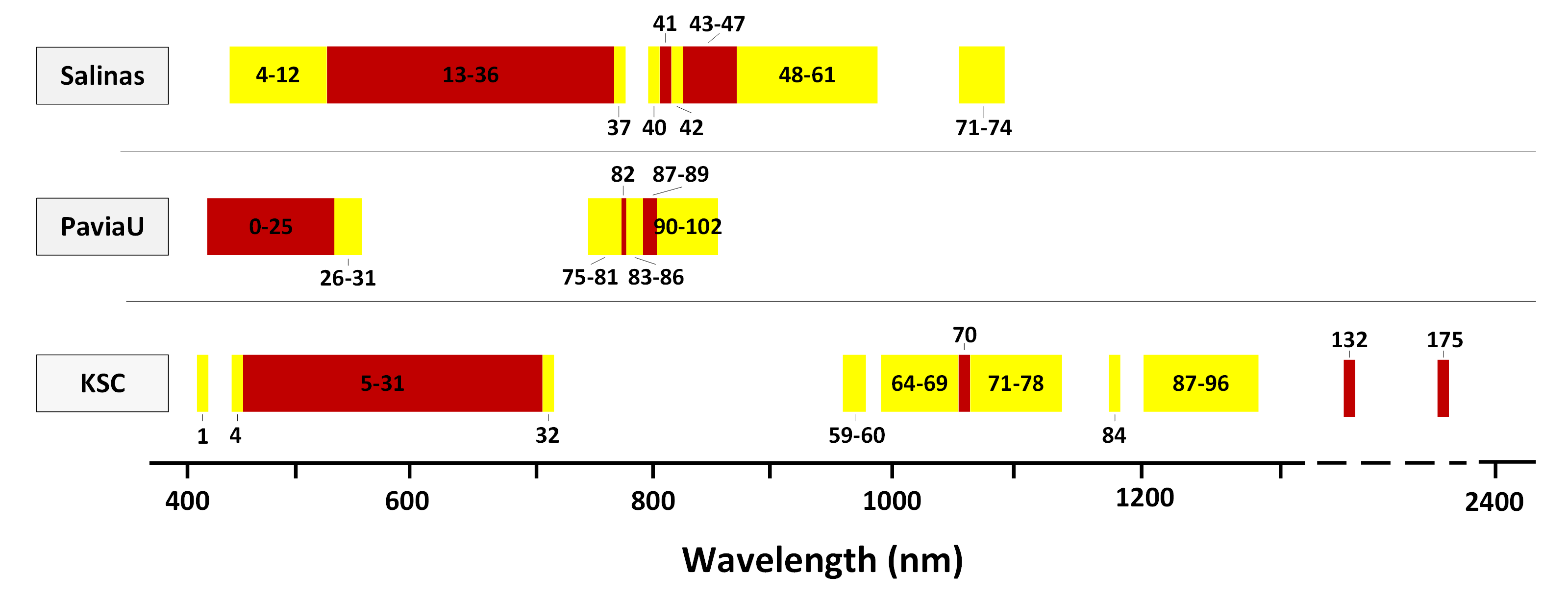
After calculating the importance scores of each band in the original data set, select the top k bands to form a new, lower-dimensional data set (which is the general processing of the ORF method). When the dimension of an HSI is required to be reduced to 30 dimensions, the 30 bands with the highest importance scores are selected. The indices of the obtained 30 bands are shown, marked with red, in Figure 4. It can be seen from the figure that most of the top 30 bands are in continuous arrangement, which was the case for all three data sets. Taking the Salinas data set as an example, the top 30 bands were 13–36, 41, and 43–47. The specific ranking of these 30 bands and their corresponding importance scores are shown in

Table 3. Indices of the top 30 bands and their scores obtained by original Relief-F (ORF).

Data Set	Band Indices	Importance Scores
Salinas	[31, 33, 30, 32, 28, 29, 34, 27, 26, 25, 24, 23, 35, 22, 21, 36, 44, 20, 43, 45, 19, 46, 41, 18, 47, 17, 14, 16, 13, 15]	[1.000, 0.988, 0.981, 0.952, 0.845, 0.837, 0.826, 0.807, 0.752, 0.750, 0.739, 0.673, 0.663, 0.638, 0.580, 0.554, 0.505, 0.499, 0.469, 0.463, 0.451, 0.447, 0.443, 0.417, 0.405, 0.391, 0.379, 0.367, 0.354, 0.343]
PaviaU	[0, 1, 2, 3, 4, 5, 6, 14, 13, 17, 7, 15, 16, 18, 20, 19, 9, 12, 8, 10, 21, 11, 22, 88, 87, 25, 89, 24, 23, 82]	[1.000, 0.571, 0.468, 0.338, 0.311, 0.301, 0.276, 0.254, 0.252, 0.243, 0.235, 0.234, 0.233, 0.233, 0.230, 0.228, 0.219, 0.216, 0.216, 0.213, 0.213, 0.201, 0.186, 0.179, 0.177, 0.174, 0.173, 0.171, 0.170, 0.169]
KSC	[175, 16, 15, 18, 13, 14, 19, 17, 20, 10, 12, 9, 11, 8, 22, 24, 21, 7, 23, 25, 132, 26, 27, 30, 29, 6, 28, 5, 31, 70]	[1.000, 0.656, 0.655, 0.640, 0.616, 0.613, 0.595, 0.593, 0.588, 0.584, 0.563, 0.523, 0.508, 0.482, 0.435, 0.430, 0.424, 0.408, 0.396, 0.375, 0.369, 0.338, 0.304, 0.291, 0.269, 0.256, 0.254, 0.238, 0.199, 0.192]

. For generality, Figure 4 also shows the indices (marked in yellow) of the bands with importance scores ranking from 31 to 60. It can be seen that, in the three data sets, most of the bands with scores ranging from 31 to 60 were still continuously arranged. In summary, most of the top k bands obtained by the general processing of the ORF are arranged continuously. The main reason for this may be that HSIs acquire narrow spectral bands over the continuous spectral range, such that the measured values between adjacent bands are similar.

The second assumption is verified in the rest of this section. In fact, it is only necessary to verify that ${\mu }_D<ϵ$, where $ϵ$ is a small real number (i.e., the difference between $error\left(b_i\right)$ and $error\left(b_i\right)$ is significantly small), without verifying ${\mu }_D=0$. The test results are shown in

Table 4. The results of the paired sample t-test, in which the significance level is $95\%$ (i.e., $\alpha =0.05$).

Data Set	${\mathit{H}}_0$	${\mathit{H}}_1$	${\overline{\mathit{X}}}_{1\mathit{i}}$	${\overline{\mathit{X}}}_{2\mathit{i}}$	t	$-{\mathit{t}}_{\mathit{\alpha }}$
Salinas	${\mu }_D\ge 0.01$	${\mu }_D\le 0.01$	0.9956	0.9910	−3.2989	−1.6524
PaviaU	${\mu }_D\ge 0.01$	${\mu }_D\le 0.01$	0.9987	0.9971	−11.6331	−1.6599
KSC	${\mu }_D\ge 0.20$	${\mu }_D\le 0.20$	0.8203	0.5920	1.1991	−1.6536

, after modifying $H_0$ and $H_1$ accordingly.

According to Table 4, there was a high correlation between adjacent bands in the two data sets (Salinas and PaviaU), which can be seen from the means of $neibor\_corr\left(x_i\right)$ in the two data sets (0.9910 and 0.9971, respectively). Paired sample t-tests show that the calculated t values of these two data sets fall into the rejection domain (i.e., we reject the null hypotheses and accept the alternative hypotheses). This shows that, in the case of the significance level $\alpha =0.05$, the difference between $max\_corr\left(x_i\right)$ and $neibor\_corr\left(x_i\right)$ is significantly small (${\mu }_D\le 0.01$). However, the mean of $neibor\_corr\left(x_i\right)$ in the KSC data set is 0.5920, which is relatively small compared to the perceived high correlation. The value of the t distribution statistic falls into the acceptance domain (i.e., the difference between $max\_corr\left(x_i\right)$ and $neibor\_corr\left(x_i\right)$ is significantly large; ${\mu }_D\ge 0.2$). According to the screening, about 37% of $neibor\_corr\left(x_i\right)$ of all adjacent bands in the KSC data set are greater than 0.98, while about 60% are less than 0.59; that is to say, some of the adjacent bands are highly correlated, while a large number of adjacent bands are not.

Generally speaking, due to the high correlation between adjacent bands, the information they contain is similar. Therefore, only selecting bands based on their importance scores will cause the selected bands to contain similar information. The band subset can have a large sum of importance scores, according to this operation; however, it does not actually contain diverse enough information, due to this similarity. Therefore, in order to ensure that the final band subset has low redundancy, our partitioning strategy is added to ensure that the selected bands are from different sub-intervals.

4.3. The Effectiveness and Advancement of the PRF Method

When using PRF to reduce the dimensionality of HSI data, the threshold $\lambda$ needs to be set in advance. The value of $\lambda$ affects the size of each sub-interval and the number of the selected bands. Therefore, this section will first explore the reasonable values of $\lambda$.

The maximum correlation coefficient between each band ($b_i$) and its adjacent bands (denoted as $neibor\_corr\left(b_i\right)$) can be calculated, according to Equation (6). Table 4 gives the average values of the respective $neibor\_corr\left(b_i\right)$ (i.e., ${\overline{X}}_{2i}$), which can be used as a reference for the value of $\lambda$. Therefore, the value of the threshold started at $0.98$ in the experiment.

According to

Table 5. Classification overall accuracy (OA) and the number of bands with different values of threshold $\lambda$, where ($1-\lambda$) is the alternative to emphasize the magnitude variation of threshold values.

$1-\mathit{\lambda }$	Salinas		PaviaU		KSC
	No. of Bands	OA	No. of Bands	OA	No. of Bands	OA
0.02	11	0.8969	5	0.852	31	0.9192
0.01	15	0.8995	8	0.8947	35	0.926
0.001	32	0.935	31	0.932	42	0.9331
0.0001	51	0.9445	46	0.9471	57	0.9405
0.00001	78	0.9415	74	0.9466	82	0.9376

, when $(1-\lambda )=0.02$, the band number of the reduced-dimensional Salinas, PaviaU, and KSC data sets were 11, 5, and 31, respectively. It can be known that the correlation between the adjacent bands of the KSC data set was far lower than that of the other two data sets based on Table 4. Therefore, though the three data sets were sharing the same threshold value, which was 0.98 (i.e., $(1-\lambda )=0.02$), the band number of the reduced-dimensional KSC data set was importantly larger than that of the other two data sets. According to the algorithm flow of PRF, the number of sub-intervals increases as the increasing threshold values; namely, the band number of the dimension-reduced data set increases accordingly. The growth of the band number allows the data sets to have more abundant information. Thus, it can be seen that the OA of the three data sets was constantly improving during the reduction of the value of ($1-\lambda$) from 0.02 to 0.0001. However, the redundancy of the reduced-dimensional data sets could be at a higher degree when the threshold values exceed a certain level. In this case, when $(1-\lambda )=0.00001$, the classification accuracy was decreased yet while the number of bands was much more than before. Similar results were obtained on these three data sets.

The PRF method partitions the bands with the partitioning strategy given in Section 3.3, where the general process is conducted in order of wavelength from short to long. We reversed the partitioning order and repeated the experiments to explore the variation of the dimensionality reduction effect of the PRF method. The experimental results are shown in

Table 6. Classification overall accuracy (OA) and the number of bands with different values of threshold $\lambda$, where the partitioning order of Partitioned Relief-F (PRF) is reversed.

$1-\mathit{\lambda }$	Salinas		PaviaU		KSC
	No. of Bands	OA	No. of Bands	OA	No. of Bands	OA
0.02	11	0.8947	4	0.8411	29	0.9064
0.01	14	0.8944	7	0.883	33	0.9091
0.001	32	0.9393	29	0.9365	43	0.9314
0.0001	52	0.9439	44	0.9473	55	0.9366
0.00001	76	0.9435	70	0.9469	81	0.9294

, which demonstrate that there are slight changes in the results when the experiment is conducted in order of wavelength from long to short. Considering the specific mechanism of the proposed partitioning strategy that adds bands into sub-intervals orderly, the obtained, different partitioning results are expectable. However, the low correlation between bands from different sub-intervals is definite, which ensures a limited variability of partitioning results. In addition, the representative bands are achieved from sub-intervals according to the importance scores in both situations; thus, a significant difference in the selection of representative bands would not be seen if there was no significant variation of the sub-intervals.

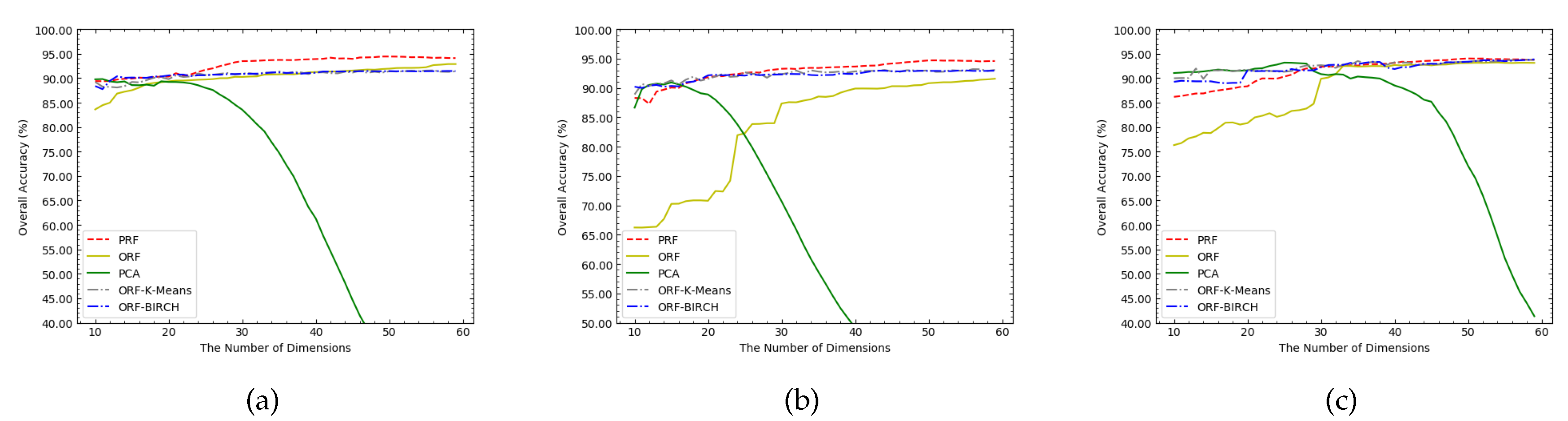
The clustering process on bands is similar to the partitioning strategy in PRF, where the clusters obtained by the clustering algorithm is similar to the sub-intervals obtained by PRF. Therefore, we chose two clustering algorithms, K-Means and BIRCH, to compare with the proposed partitioning strategy. Both the K-Means and BIRCH algorithms need to specify the number of clusters in advance, and the representative bands are selected from each cluster, where the representative bands are also obtained based on the importance scores. Therefore, the band selection methods based on these two clustering algorithms are denoted as ORF-K-Means and ORF-BIRCH, respectively. The five methods, ORF, PCA, ORF-K-Means, ORF-BIRCH, and PRF, are examined for the situation that the effect of dimensionality reduction changes with an increase of the number of bands, as shown in Figure 5.

On the three data sets, the classification accuracy based on PCA showed an obvious trend of first rising and then falling. The ORF method had extremely poor performance in low dimensions, which was particularly reflected in the PaviaU and KSC data sets. With an increase of dimensionality, the OA of ORF-based classification continued to improve. However, after the dimensionality reached 40, its OA increased slowly. When using K-Means or BIRCH to cluster the bands before the band selection, it can be found that the effect was better than ORF. After adding the partitioning strategy, it can be seen that the classification model achieved a high OA in low dimensions, which means that the partitioning strategy can effectively solve the problem of the deficiency of the available information (i.e., diverse information) due to the redundancy of bands.

According to Figure 5, it can be seen that PRF had obvious advantages in the Salinas and PaviaU data sets, while its advantage on KSC was relatively weak. According to the test results in Table 5, the correlation between bands in the Salinas and PaviaU data sets reached a very high level, while the correlation in the KSC data set was relatively low (Salinas: 0.9910; PaviaU: 0.9971; KSC: 0.5920). The partitioning strategy mainly divides the sub-intervals based on the correlation between bands; therefore, the partitioning strategy performed better in the Salinas and PaviaU data sets than in the KSC data set.

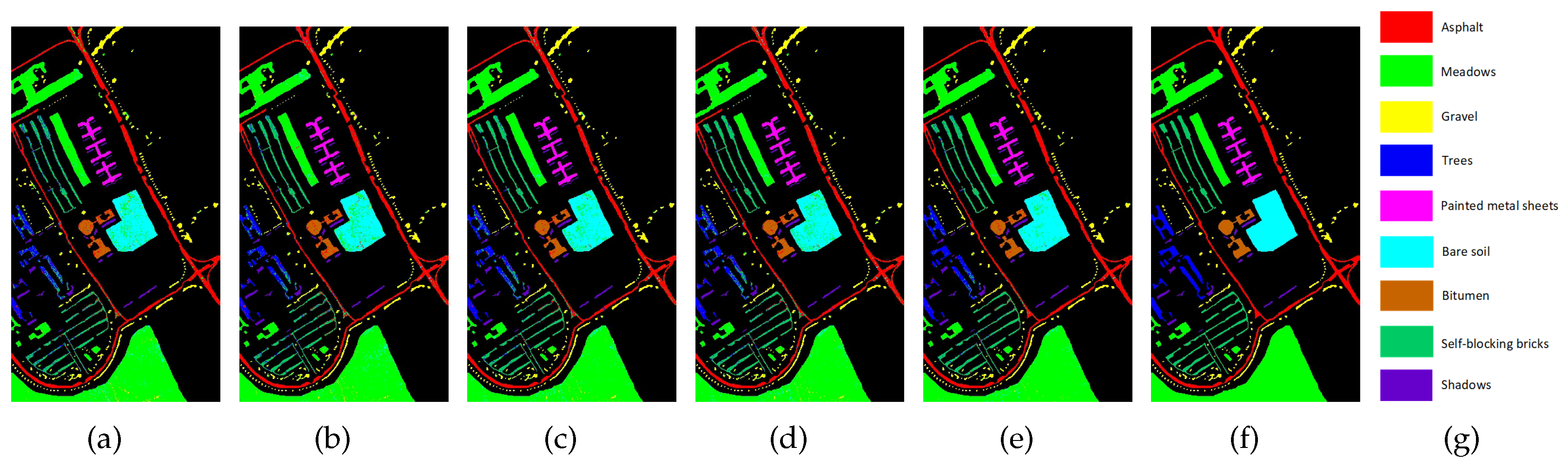
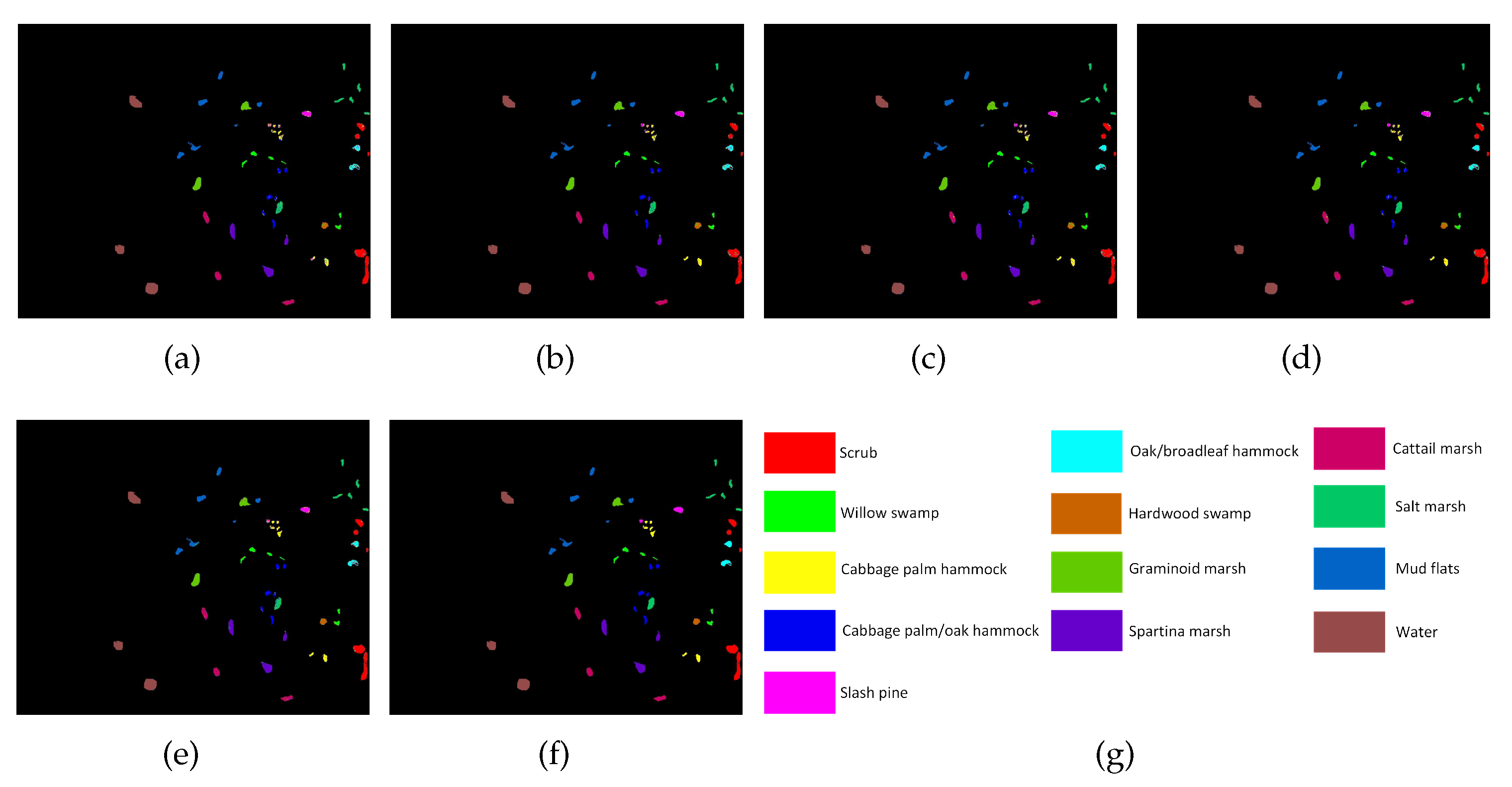
Classification maps for the three data sets obtained by different methods are shown in Figure 6a–e, Figure 7a–e, and Figure 8a–e, where all the maps had classification noise. Figure 6a–e contains classification maps for the Salinas data set, where the noise was mainly concentrated in two regions that belong to Vineyard-untrained and Grapes-untrained, respectively. Figure 7a–e contains classification maps for the PaviaU data set, where the noise was mainly concentrated in the region belonging to Bare soil. Figure 8a–e contains classification maps for the KSC data set, where the noise was mainly concentrated in three regions that belong to Cabbage palm hammock, Slash pine, and Scrub, respectively. In summary, subfigure (e) contained less noise than the other four subfigures, which was shown in all three figures; that is, the PRF method performed better than the other four methods.

More specifically, the optimal classifications based on various methods were compared, as shown in

Table 7. Optimal classification results based on different dimensionality reduction methods.

	ORF	PCA	ORF-K-Means	ORF-BIRCH	PRF
Salinas	92.90	89.82	91.58	91.48	94.45
PaviaU	91.57	90.94	93.21	92.99	94.71
KSC	93.22	93.19	93.77	93.87	94.05

. It can be seen that, compared with the other four methods, the PRF-based classification model obtained the optimal OA in the three data sets. In the PaviaU and KSC data sets, the OA of the classification model based on K-Means (or BIRCH) was better than that based on ORF. In general, the partitioning strategies effectively improved the performance of dimensionality reduction for HSIs, especially the partitioning strategy proposed in Section 3.3.

Finally, the runtimes of the various methods were analyzed, as shown in

Table 8. Runtimes of various methods (s).

	ORF	PCA	ORF-K-Means	ORF-BIRCH	PRF
Salinas	7.34	0.57	19.06	9.64	7.99
PaviaU	1.67	0.33	6.49	2.22	1.87
KSC	2.37	0.05	3.28	2.53	2.41

. In the three data sets, as the Salinas data set had the largest number of bands and samples, each method had the longest runtime on it. As the number of bands in the KSC data set was more than that of the PaviaU data set, the runtimes of the ORF and PRF methods on the KSC data set were longer than that on the PaviaU data set. In general, the runtime of PCA was the shortest, and the runtime of PRF was less than those of K-Means and BIRCH.

5. Conclusions

In this paper, we proposed a classification model for HSI data sets of small size. Our main focus was to provide a dimensionality reduction method combining the Relief-F method and a partitioning strategy, where the Relief-F method is used to calculate the importance score of each band. A partitioning strategy was proposed to divide the band interval, in order to reduce the redundancy of the selected bands. The main idea of the partitioning strategy was to divide the entire band interval into various sub-intervals that have high redundancy, which ultimately ensures that the bands selected from the sub-intervals are less redundant.

The effectiveness of the method provided in this paper was tested by experiments on three data sets. In the experiments, the high correlation between adjacent bands in the HSI data sets was first verified, and the shortcomings of the ORF method in the band selection strategy were analyzed. Compared with the ORF and PCA methods, the advantages of PRF were verified in the HSI data sets with highly correlated adjacent bands. In addition, the K-Means and BIRCH clustering methods were also used for comparison. The experimental results show that the division of the band interval can effectively reduce the redundancy between the selected bands, and that the partitioning strategy proposed in this paper is particularly effective. The method proposed in this paper has not yet been used to mine the spatial information of HSIs. Therefore, we will focus on the integration of spatial information into the feature selection method in future work.

References

- Chutia, D.; Bhattacharyya, D.K.; Sarma, K.K.; Kalita, R.; Sudhakar, S. Hyperspectral remote sensing classifications: A perspective survey. Trans. GIS 2015, 20, 463–490. [Google Scholar] [CrossRef]
- Benediktsson, J.A.; Palmason, J.A.; Sveinsson, J.R. Classification of hyperspectral data from urban areas based on extended morphological profiles. IEEE Trans. Geosci. Remote Sens. 2005, 43, 480–491. [Google Scholar] [CrossRef]
- Fauvel, M.; Tarabalka, Y.; Benediktsson, J.A.; Chanussot, J.; Tilton, J.C. Advances in spectral-spatial classification of hyperspectral images. Proc. IEEE 2013, 101, 652–675. [Google Scholar] [CrossRef] [Green Version]
- Bellman, R.E. Rand Corporation. Dynamic Programming; Princeton University Press: Princeton, NJ, USA, 1957. [Google Scholar]
- Chang, C.I. Hyperspectral Data Exploitation: Theory and Applications; John Wiley & Sons: Hoboken, NJ, USA, 2007. [Google Scholar]
- Bioucas-Dias, J.M.; Plaza, A.; Camps-Valls, G.; Scheunders, P.; Nasrabadi, N.; Chanussot, J. Hyperspectral remote sensing data analysis and future challenges. IEEE Geosci. Remote Sens. Mag. 2013, 1, 6–36. [Google Scholar] [CrossRef] [Green Version]
- Jiang, J.; Ma, J.; Chen, C.; Wang, Z.; Cai, Z.; Wang, L. SuperPCA: A superpixelwise PCA approach for unsupervised feature extraction of hyperspectral imagery. IEEE Trans. Geosci. Remote Sens. 2018, 56, 4581–4593. [Google Scholar] [CrossRef] [Green Version]
- Marcinkowska-Ochtyra, A.; Zagajewski, B.; Ochtyra, A.; Jarocińska, A.; Wojtuń, B.; Rogass, C.; Mielke, C.; Lavender, S. Subalpine and alpine vegetation classification based on hyperspectral APEX and simulated EnMAP images. Int. J. Remote Sens. 2007, 38, 1839–1864. [Google Scholar] [CrossRef] [Green Version]
- Wang, J.; Chang, C.I. Independent component analysis-based dimensionality reduction with applications in hyperspectral image analysis. IEEE Trans. Geosci. Remote Sens. 2006, 44, 1586–1600. [Google Scholar] [CrossRef]
- Wang, Q.; Meng, Z.; Li, X. Locality adaptive discriminant analysis for spectral–spatial classification of hyperspectral images. IEEE Geosci. Remote Sens. Lett. 2017, 14, 2077–2081. [Google Scholar] [CrossRef]
- Chaudhari, A.J.; Darvas, F.; Bading, J.R.; Moats, R.A.; Conti, P.S.; Smith, D.J.; Cherry, S.R.; Leahy, R.M. Hyperspectral and multispectral bioluminescence optical tomography for small animal imaging. Phys. Med. Biol. 2005, 50, 5421–5441. [Google Scholar] [CrossRef]
- Bruce, L.M.; Koger, C.H.; Li, J. Dimensionality reduction of hyperspectral data using discrete wavelet transform feature extraction. IEEE Trans. Geosci. Remote Sens. 2002, 40, 2331–2338. [Google Scholar] [CrossRef]
- Jiang, Y.L.; Zhang, R.Y.; Yu, J.; Hu, W.C.; Yin, Z.T. Detection of infected tephritidae citrus fruit based on hyperspectral imaging and two-band ratio algorithm. Adv. Mater. Res. Trans. Tech. Publ. 2011, 311, 1501–1504. [Google Scholar] [CrossRef]
- Cao, X.; Wu, B.; Tao, D.; Jiao, L. Automatic band selection using spatial-structure information and classifier-based clustering. IEEE J. Sel. Top. Appl. Earth Obs. Remote Sens. 2016, 9, 4352–4360. [Google Scholar] [CrossRef]
- Hamada, Y.; Stow, D.A.; Coulter, L.L.; Jafolla, J.C.; Hendricks, L.W. Detecting Tamarisk species (Tamarix spp.) in riparian habitats of Southern California using high spatial resolution hyperspectral imagery. Remote Sens. Environ. 2007, 109, 237–248. [Google Scholar] [CrossRef]
- Su, H.; Yang, H.; Du, Q.; Sheng, Y. Semisupervised band clustering for dimensionality reduction of hyperspectral imagery. IEEE Geosci. Remote Sens. Lett. 2011, 8, 1135–1139. [Google Scholar] [CrossRef]
- Su, H.; Du, Q.; Chen, G.; Du, P. Optimized hyperspectral band selection using particle swarm optimization. IEEE J. Sel. Top. Appl. Earth Obs. Remote Sens. 2014, 7, 2659–2670. [Google Scholar] [CrossRef]
- Cen, H.; Lu, R.; Zhu, Q.; Mendoza, F. Nondestructive detection of chilling injury in cucumber fruit using hyperspectral imaging with feature selection and supervised classification. Postharvest Biol. Technol. 2016, 111, 352–361. [Google Scholar] [CrossRef]
- Deronde, B.; Kempeneers, P.; Forster, R.M. Imaging spectroscopy as a tool to study sediment characteristics on a tidal sandbank in the Westerschelde. Estuar. Coast. Shelf Sci. 2006, 69, 580–590. [Google Scholar] [CrossRef]
- Serpico, S.B.; Bruzzone, L. A new search algorithm for feature selection in hyperspectral remote sensing images. IEEE Trans. Geosci. Remote Sens. 2001, 39, 1360–1367. [Google Scholar] [CrossRef]
- Huang, W.; Guan, Q.; Luo, J.; Zhang, J.; Zhao, J.; Liang, D.; Huang, L.; Zhang, D. New optimized spectral indices for identifying and monitoring winter wheat diseases. IEEE J. Sel. Top. Appl. Earth Obs. Remote Sens. 2014, 7, 2516–2524. [Google Scholar] [CrossRef]
- Pal, M.; Mather, P.M. Support vector machines for classification in remote sensing. Int. J. Remote Sens. 2005, 26, 1007–1011. [Google Scholar] [CrossRef]
- Nielsen, A.A. Kernel maximum autocorrelation factor and minimum noise fraction transformations. IEEE Trans. Image Process. 2010, 20, 612–624. [Google Scholar] [CrossRef] [Green Version]
- Fauvel, M.; Chanussot, J.; Benediktsson, J.A. Kernel Principal Component Analysis for Feature Reduction in Hyperspectrale Images Analysis. In Proceedings of the 7th Nordic Signal Processing Symposium-NORSIG 2006, Rejkjavik, Iceland, 7–9 June 2006; pp. 238–241. [Google Scholar]
- Li, X.; Zhang, L.; You, J. Hyperspectral Image Classification Based on Two-Stage Subspace Projection. Remote Sens. 2018, 10, 1565. [Google Scholar] [CrossRef] [Green Version]
- Zhang, L.; Su, H.; Shen, J. Hyperspectral Dimensionality Reduction Based on Multiscale Superpixelwise Kernel Principal Component Analysis. Remote Sens. 2019, 11, 1219. [Google Scholar] [CrossRef] [Green Version]
- Binol, H. Ensemble Learning Based Multiple Kernel Principal Component Analysis for Dimensionality Reduction and Classification of Hyperspectral Imagery. Math. Probl. Eng. 2018, 2018, 9632569. [Google Scholar] [CrossRef]
- Zhao, B.; Gao, L.; Zhang, B. An Optimized Method of Kernel Minimum noise Fraction for Dimensionality Reduction of Hyperspectral Imagery. In Proceedings of the 2016 IEEE International Geoscience and Remote Sensing Symposium (IGARSS), Beijing, China, 10–15 July 2016; pp. 48–51. [Google Scholar]
- Gómez-Chova, L.; Nielsen, A.A.; Camps-Valls, G. Explicit Signal to Noise Ratio in Reproducing Kernel Hilbert Spaces. In Proceedings of the 2011 IEEE International Geoscience and Remote Sensing Symposium, Vancouver, BC, Canada, 24–29 July 2011; pp. 3570–3573. [Google Scholar]
- Song, S.; Zhou, H.; Qin, H.; Qian, K.; Cheng, K.; Qian, J. Hyperspectral Image Anomaly Detecting Based on Kernel Independent Component Analysis. In Proceedings of the Fourth Seminar on Novel Optoelectronic Detection Technology and Application, Nanjing, China, 24–26 October 2017. [Google Scholar]
- Han, Z.; Wan, J.; Deng, L.; Liu, K. Oil Adulteration identification by hyperspectral imaging using QHM and ICA. PLoS ONE 2016, 11, e0146547. [Google Scholar] [CrossRef] [PubMed] [Green Version]
- Yuan, H.; Tang, Y.Y.; Lu, Y.; Yang, L.; Luo, H. Spectral-spatial classification of hyperspectral image based on discriminant analysis. IEEE J. Sel. Top. Appl. Earth Obs. Remote Sens. 2013, 7, 2035–2043. [Google Scholar] [CrossRef]
- Gu, Y.; Zhang, L. Rare signal component extraction based on kernel methods for anomaly detection in hyperspectral imagery. Neurocomputing 2013, 108, 103–110. [Google Scholar] [CrossRef]
- Du, P.; Tan, K.; Xing, X. Wavelet SVM in reproducing kernel Hilbert space for hyperspectral remote sensing image classification. Opt. Commun. 2010, 283, 4978–4984. [Google Scholar] [CrossRef]
- Tenenbaum, J.B.; De Silva, V.; Langford, J.C. A global geometric framework for nonlinear dimensionality reduction. Science 2000, 290, 2319–2323. [Google Scholar] [CrossRef]
- Orts Gomez, F.J.; Ortega López, G.; Filatovas, E.; Kurasova, O.; Garzón, G.E.M. Hyperspectral Image Classification Using Isomap with SMACOF. Informatica 2019, 30, 349–365. [Google Scholar]
- Songyang, Z.; Kun, T.; Lixin, W. Hyperspectral image classification based on ISOMAP algorithm using neighborhood distance. Remote Sens. Technol. Appl. 2014, 29, 695–700. [Google Scholar]
- Yan, L.; Roy, D.P. Improved time series land cover classification by missing-observation-adaptive nonlinear dimensionality reduction. Remote Sens. Environ. 2015, 158, 478–491. [Google Scholar] [CrossRef] [Green Version]
- Qian, S.E.; Chen, G. A New Nonlinear Dimensionality Reduction Method with Application to Hyperspectral Image Analysis. In Proceedings of the 2007 IEEE International Geoscience and Remote Sensing Symposium, Barcelona, Spain, 23–28 July 2007; pp. 270–273. [Google Scholar]
- Feng, F.; Li, W.; Du, Q.; Zhang, B. Dimensionality reduction of hyperspectral image with graph-based discriminant analysis considering spectral similarity. Remote Sens. 2017, 9, 323. [Google Scholar] [CrossRef] [Green Version]
- Sun, W.; Du, Q. Hyperspectral band selection: A review. IEEE Geosci. Remote Sens. Mag. 2019, 7, 118–139. [Google Scholar] [CrossRef]
- Shafri, H.Z.M.; Anuar, M.I.; Saripan, M.I. Modified vegetation indices for Ganoderma disease detection in oil palm from field spectroradiometer data. J. Appl. Remote Sens. 2009, 3, 033556. [Google Scholar]
- Du, Z.; Jeong, M.K.; Kong, S.G. Band selection of hyperspectral images for automatic detection of poultry skin tumors. IEEE Trans. Autom. Sci. Eng. 2007, 4, 332–339. [Google Scholar] [CrossRef]
- Mahlein, A.K.; Rumpf, T.; Welke, P.; Dehne, H.W.; Plümer, L.; Steiner, U.; Oerke, E.C. Development of spectral indices for detecting and identifying plant diseases. Remote Sens. Environ. 2013, 128, 21–30. [Google Scholar]
- Du, Q. A new sequential algorithm for hyperspectral endmember extraction. IEEE Geosci. Remote Sens. Lett. 2012, 9, 695–699. [Google Scholar]
- Sun, K.; Geng, X.; Ji, L.; Lu, Y. A new band selection method for hyperspectral image based on data quality. IEEE J. Sel. Top. Appl. Earth Obs. Remote Sens. 2014, 7, 2697–2703. [Google Scholar]
- Ghamisi, P.; Couceiro, M.S.; Benediktsson, J.A. A novel feature selection approach based on FODPSO and SVM. IEEE Trans. Geosci. Remote Sens. 2014, 53, 2935–2947. [Google Scholar] [CrossRef] [Green Version]
- Vaiphasa, C.; Skidmore, A.K.; de Boer, W.F.; Vaiphasa, T. A hyperspectral band selector for plant species discrimination. ISPRS J. Photogramm. Remote Sens. 2007, 62, 225–235. [Google Scholar] [CrossRef]
- MartÍnez-UsÓMartinez-Uso, A.; Pla, F.; Sotoca, J.M.; García-Sevilla, P. Clustering-based hyperspectral band selection using information measures. IEEE Trans. Geosci. Remote Sens. 2007, 45, 4158–4171. [Google Scholar] [CrossRef]
- Imbiriba, T.; Bermudez, J.C.M.; Richard, C.; Tourneret, J.Y. Band Selection in RKHS for Fast Nonlinear Unmixing of Hyperspectral Images. In Proceedings of the 2015 23rd European Signal Processing Conference (EUSIPCO), Nice, France, 31 August–4 September 2015; pp. 1651–1655. [Google Scholar]
- Li, S.; Qi, H. Sparse Representation Based Band Selection for Hyperspectral Images. In Proceedings of the 2011 18th IEEE International Conference on Image Processing, Brussels, Belgium, 11–14 September 2016; pp. 2693–2696. [Google Scholar]
- Sun, W.; Jiang, M.; Li, W.; Liu, Y. A symmetric sparse representation based band selection method for hyperspectral imagery classification. Remote Sens. 2016, 8, 238. [Google Scholar] [CrossRef] [Green Version]
- Zhang, T.; Ramakrishnan, R.; Livny, M. BIRCH: An efficient data clustering method for very large databases. ACM Sigmod Rec. 1996, 25, 103–114. [Google Scholar] [CrossRef]
Figure 1.
Structure of the proposed model for HSI dimensionality reduction.
Figure 2.
Schematic of the partitioning strategy.
Figure 3.
Flowchart of data processing, where Processing (1) is the processing performed by the data provider and Processing (2) is the processing performed in this paper.
Figure 4.
Schematic of band selection using ORF method, where the red part represents the top 30 bands according to importance scores, the yellow part represents the bands with scores ranking from 31 to 60, and the numbers represent the indices of each band.
Figure 5.
The classification overall accuracy (OA) changes under different dimensions of the subsets and different dimensionality reduction methods. The three data sets Salinas, PaviaU, and KSC are marked by (a), (b), and (c), respectively.
Figure 6.
Classification maps for the Salinas data set obtained by different methods: (a) PCA; (b) ORF; (c) ORF-K-Means; (d) ORF-BIRCH; (e) PRF. In addition, (f) is the ground truth, and (g) is the legend.
Figure 7.
Classification maps for the PaviaU data set obtained by different methods: (a) PCA; (b) ORF; (c) ORF-K-Means; (d) ORF-BIRCH; (e) PRF. In addition, (f) is the ground truth, and (g) is the legend.
Figure 8.
Classification maps for the Kennedy Space Center (KSC) data set obtained by different methods: (a) PCA; (b) ORF; (c) ORF-K-Means; (d) ORF-BIRCH; (e) PRF. In addition, (f) is the ground truth, and (g) is the legend.