OCO-2 Solar-Induced Chlorophyll Fluorescence Variability across Ecoregions of the Amazon Basin and the Extreme Drought Effects of El Niño (2015–2016)

Abstract

Amazonian ecosystems are major biodiversity hotspots and carbon sinks that may lose species to extinction and become carbon sources due to extreme dry or warm conditions. We investigated the seasonal patterns of high-resolution solar-induced chlorophyll fluorescence (SIF) measured by the satellite Orbiting Carbon Observatory-2 (OCO-2) across the Amazonian ecoregions to assess the area´s phenology and extreme drought vulnerability. SIF is an indicator of the photosynthetic activity of chlorophyll molecules and is assumed to be directly related to gross primary production (GPP). We analyzed SIF variability in the Amazon basin during the period between September 2014 and December 2018. In particular, we focused on the SIF drought response under the extreme drought period during the strong El Niño in 2015–2016, as well as the 6-month drought peak period. During the drought´s peak months, the SIF decreased and increased with different intensities across the ecoregions of the Amazonian moist broadleaf forest (MBF) biome. Under a high temperature, a high vapor pressure deficit, and extreme drought conditions, the SIF presented differences from −31.1% to +17.6%. Such chlorophyll activity variations have been observed in plant-level measurements of active fluorescence in plants undergoing physiological responses to water or heat stress. Thus, it is plausible that the SIF variations in the ecoregions’ ecosystems occurred as a result of water and heat stress, and arguably because of drought-driven vegetation mortality and collateral effects in their species composition and community structures. The SIF responses to drought at the ecoregional scale indicate that there are different levels of resilience to drought across MBF ecosystems that the currently used climate- and biome-region scales do not capture. Finally, we identified monthly SIF values of 32 ecoregions, including non-MBF biomes, which may give the first insights into the photosynthetic activity dynamics of Amazonian ecoregions.

1. Introduction

Vegetation in the Amazon region is highly diverse and contains about one-half of the biomass stored in tropical forests [1,2]. Tropical forests play an important role in the global carbon cycle by intaking up to ~1.2 Pg of carbon (C) per year [3]. In recent decades, the Amazon region was hit by repeated severe drought events in 2005, 2010, and 2015–2016 [4,5,6]. Such events have the potential to alter the carbon cycle of the Amazon rainforest through biomass losses from, for example, increased tree mortality, and may thus lead to increased carbon emissions to the atmosphere [5,6].

For the 2005 and 2010 droughts, C emissions from the Amazon rainforest were estimated to be ~1.6 Pg C and ~2.2 Pg C, respectively [5]. During the period from September 2015 to March 2016, the terrestrial water storage in the Amazon basin was lower by one standard deviation (sd) than the 1900–2016 climatological seasonal cycle, and in August 2016, the rainfall remained 10% below the average values, leading to strong reductions in gross primary productivity (GPP; [7]). Such repeated drought events have the potential to turn the forest into a C source [5,8]. Quantifying the GPP for the Amazon region remains a challenge due to the area´s large spatial extent, remote field sites, and difficulties in installing long-term monitoring sites. Only recently have remotely sensed solar-induced chlorophyll fluorescence (SIF) tools become available, which may help overcome spatial and temporal gaps in the model-based up-scaling of GPP fluxes from eddy covariance measurements.

SIF refers to the fluorescence radiance (photons) emitted from the chlorophyll molecules during plant photosynthesis. The emitted fluorescence wavelength ranges up to 600–850 nm, and constitutes both photosystems (I and II). This is proposed to be a remote sensing proxy for gross photosynthesis [9] that allows the constraining of carbon balance estimates [10]. The remotely sensed GOME-2 mission’s SIF and the GPP measured using a network of carbon flux towers (FLUXNET-GPP) show a high correlation globally (r² = 0.74), albeit with regional variations [11]. For the Amazon region, high correlations (Pearson correlation coefficient = 0.80) were found between GOME-2’s SIF, and an up-scaled GPP product that extrapolated the eddy covariance estimations using machine learning [7]. Within the Amazonian region, the phenological seasonality in vegetation communities has been attributed to climate factors; 76% of the SIF seasonality of Amazonia is explained by seasonal radiation variation, while 13% and 11% are explained by precipitation and a combination of both [12]. In contrast, when vegetation factors are disentangled from the climate variability of multiple forest types, two-thirds of Amazonian GPP variations are shown to be due to a forest´s composition, structure, and nutrients, while just one-third is due to intra-annual climate variability [13]. Such GPP patterns agree with remotely sensed SIF from the GOSAT satellite [13].

The photons take in by the photosystems of plants rely on the incident photosynthetically active radiation (PAR) and the fraction of that radiance absorbed by the leaves (fPAR). The PAR absorbed by leaves is partitioned into photochemistry, heat dissipation (non-photochemical quenching; NPQ), and fluorescence emission (SIF). In general, SIF satellite measurements at the canopy surface result from the absorbed photosynthetically active radiation (APAR; the combination of fPAR and PAR), the fluorescence quantum yield in the band of measurement (${\mathsf{\Phi }}_F$), and the probability that photons can escape the canopy (Equation (1); ${\Omega }_C$, [9]):

$$SIF=PAR·fPAR·{\mathsf{\Phi }}_F·{\Omega }_C$$

(1)

In canopies of temperate forests, APAR has been found to explain 85% of the variance in SIF [14], but the evaluation of SIF can be very challenging for a complex canopy (such as tropical ones; [9]). ${\mathsf{\Phi }}_F$ is genotype-dependent and affected by shading [15] and by nitrogen availability [16]. The findings on the genotype dependency of vegetation fluorescence quantum yield in the band of 692 nm [15] suggest that floristic composition may define the ${\mathsf{\Phi }}_F$ of the forest. ${\mathsf{\Phi }}_F$ differences are particularly pronounced between species with different CO₂ fixation paths (C3, C4, and CAM paths; [15]), while the shading-sensibility suggests that the depth of the forest canopy, the forest structure, and the variations in leaf display (physical shade precursors) are more related to ${\Omega }_C$ (Equation (1); [9]).

In plants, stress response strategies, such as the adjustment of their stomatal morphology and changes in their photosynthetic functions, affect the photosynthetic light use efficiency (LUE, [17]), which in turn may affect the SIF´s relationship with the GPP [9]. However, with satellite-based SIF measurements, it is not possible to measure LUE [18] or differentiate its effects on the SIF from the effect of ${\mathsf{\Phi }}_F$ and ${\Omega }_C$; only the total SIF radiance over the canopy can be studied [9,19]. SIF radiance´s relationship with GPP, which is more mechanically detailed, involves processes including energy partitioning between photosystems I and II, the fluorescence properties of these two photosystems, the canopy structure, the CO2 fixation paths, photorespiration, linear and cyclic electron transports, stoichiometry, and fluorescence radiative transfer modeling in canopies [20]. Biochemical and biophysical responses to drought at the plant level through enzymatic activity leads to changes in leaf biochemistry [21] and reductions in stomatal and mesophyll conductance [22], which result in a lower CO₂ uptake. A reduced CO₂ uptake limits photosynthetic activity and results in lower SIF values. Drought can also cause mortality via carbon starvation, hydraulic failure, and phloem transport failure [23], which alter the ecological balance by shifting the composition of vegetation communities [24,25,26,27].

In 2009, the first global satellite SIF measurements were obtained from the GOSAT mission instruments [28]; since then, SIF has been employed to study drought´s impacts on vegetation [7,29] and to assess the diversity in leaf phenology [13,30] across Amazonia. GOSAT-SIF data reveal a productivity reduction of 15% based on the GPP in Amazonia during the 2010 extreme drought event [29]. A new retrieval product based on GOME-2’s SIF showed reductions of up to 10%–15% in the eastern part and up to 2%–5% in the western part throughout the El Niño 2015–2016 extreme drought [7]. Further, during the 2015–2016 El Niño, the SIF was below its climatological range, and its reduction was particularly strong in regions with high temperatures and low water availability [7].

The recent NASA Orbiting Carbon Observatory-2 (OCO-2) mission (launched in September, 2014) [31,32,33,34,35,36,37] offers a higher-resolution alternative (footprint of 2.25 × 1.3 km) than the previous coarser SIF measurements [38] by GOSAT (footprint of 10 km diameter) [28,39] and GOME-2 (40 × 40 km) [40]. Along with a high spatial resolution, OCO-2’s SIF provides the opportunity to study the vegetation responses of specific vegetation types to different climate conditions, thus providing completely new perspectives for SIF analysis [20,41].

High-resolution SIF products, such as OCO-2, have the potential to resolve climatic and vegetation type-specific responses to water and heat stress [20], such as at the ecoregional scale. Ecoregions (ERs) can be defined as units of land containing a distinct assemblage of species and natural communities of all taxa (beyond plants taxa) with boundaries that approximate the original extent of the natural communities prior to major land-use changes [42]. For Latin America and the Caribbean, these boundaries rely on the delineations of major ecosystem types (e.g., tropical broadleaf or tropical template forests), which contain biomes (e.g., within tropical broadleaf forests there are moist or dry broadleaf forests, which have also been referred to [43] as major habitat types). These biomes are a set of ERs that meet climatic, biological, and ecological criteria (

Table 1. Dimensions for defining biomes and ERs according to Dinerstein et al. (1995).

Dimension	Biomes	ER
Climatic	Experience comparable climatic regimes	Have similar environmental conditions
Biologic	Have similar vegetation structure	Share a large majority of their species
Ecologic	Display similar spatial patterns of biodiversity (e.g., levels of beta diversity)	Interact ecologically in ways that are critical for their long-term persistence
	Contain flora and fauna with similar guild structures and life histories

).

Although recognized at coarse global biophysical scales [11,30,44], the SIF variability across more specific vegetation types (e.g., the ER from [42]) remains unresolved. Hence, in this study, we analyze the high-resolution OCO2-SIF response across different ERs of the Amazon basin to investigate SIF´s seasonal phenology patterns. Additionally, we focus on the impact of the 2015–2016 El Niño drought event on SIF.

Specifically the study aims to (1) depict SIF diversity across forest stands at the climate and ER scale, (2) discuss Amazonian phenological dynamics through an analysis of SIF in relation to fPAR, (3) present the drought temporal and spatial extent and development, and (4) estimate the drought-driven responses of SIF within each MBF-ER by relating it to environmental variables such as the vapor pressure deficit (VPD), the temperature, and the fraction of APAR (fPAR).

2. Materials and Methods

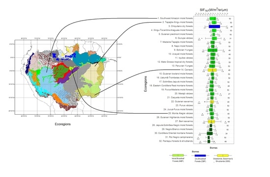
2.1. Study Region

The study region is the Amazon river basin according to the LBA-ECO CD-06 Amazon River Basin Land and Stream Drainage Direction Maps [45]. We sub-divide the Amazon basin into 47 ERs, six biomes and 14 climate zones. For these map delineations, we rely on the ER [42] and biome regions [43] derived from the RESOLVE Ecoregions 2017 data products [46] and the updated world map of the Köppen–Geiger (KG) climate classification at a 10-km spatial resolution [47] for the climate zones (KG-climate zones). A combination of the classes of these three maps is shown in Figure 1 and Appendix A

Table A1. Biomes, ecoregions (ERs) and Köppen–Geiger climate zones of the study area. Classifications are based on those of Dinerstein et al. (1995) and Kottek et al. (2006). The Köppen–Geiger classification codes consist of 2 or 3 letters describing the prevalent climate conditions (tropical [A], arid [B], warm temperate [C], snow [D], and polar [E]), precipitation (desert [W], steppe [S], fully humid [f], summer dry [s], winter dry [w], and monsoonal [m]) and temperature (hot arid [h], cold arid [k], hot summer [a], warm summer [b] and cool summer [c], and polar tundra [T]).

Biome	ER	Köppen–Geiger Climate Zone(s)
Moist Broadleaf Forests (MBFs)	Bolivian Yungas	Af - Am - Aw - BWh - BSk - Cfc - Cfa - Cfb - Cwb - Cwc - ET
	Caqueta moist forests	Af - Am
	Cordillera Oriental montane forests	Af - Am - Cfb
	Eastern Cordillera Real montane forests	Af - Am - Aw - BWh - As - Cfc - Cfb - Cwb - ET
	Guianan Highland moist forests	Af - Am - Aw - Cfb
	Guianan lowland moist forests	Af - Am - Aw
	Guianan piedmont moist forests	Af - Am - Aw - Cfb
	Gurupa várzea	Am - Aw
	Iquitos várzea	Af - Am - Aw
	Japurá–Solimões–Negro moist forests	Af
	Juruá–Purus moist forests	Af - Am - Aw
	Madeira–Tapajós moist forests	Af - Am - Aw
	Magdalena Valley montane forests	Af - Cfb
	Marajó várzea	Af - Am - Aw
	Marañón dry forests	Af - Am - Aw - BWh - BSk - Cfb - Cwb - Cwc - ET
	Mato Grosso tropical dry forests	Am - Aw
	Monte Alegre várzea	Af - Am - Aw
	Napo moist forests	Af - Am - As
	Negro–Branco moist forests	Af - Am - Cfb
	Northwest Andean montane forests	Cfc - Cfb - ET
	Pantepui forests and shrublands	Af - Am - Cfb
	Peruvian Yungas	Af - Am - Aw - BWh - BSk - Cfc - Cfb - Cwc - Cwb - ET
	Purus–Madeira moist forests	Af - Am - Aw
	Purus várzea	Af - Am - Aw
	Rio Negro campinarana	Af - Am
	Solimões–Japurá moist forests	Af
	Southern Andean Yungas	Aw - BWh - BSk - Cfa- Cfb - Cwa - Cwb
	Southwest Amazon moist forests	Af - Am - Aw - BWh - Cfb
	Tapajós–Xingu moist forests	Am - Aw
	Uatumã–Trombetas moist forests	Af - Am - Aw
	Ucayali moist forests	Af - Am - Aw - Cfb
	Xingu-Tocantins-Araguaia moist forests	Af - Am - Aw
Dry Broadleaf Forests (DBFs)	Beni savanna	Af - Am - Aw
	Bolivian montane dry forests	Aw - BWh - BSk - ET - Cfb - Cwb
	Chiquitano dry forests	Am - Aw
	Magdalena Valley dry forests	Af - Cfb
	Tumbes–Piura dry forests	Cfb - Cwb - ET
Grasslands, Savannas and Shrublands (GSSs)	Central Andean dry puna	BSk - Cwc - Cwb - ET
	Cerrado	Aw
	Dry Chaco	BWh - Aw
	Guianan savanna	Af - Am - Aw
Montane Grasslands and Shrublands (MGSs)	Central Andean puna	BSk - BWh - Cfb - Cfc - Cwc - Cwb - ET
	Central Andean wet puna	ET - Cfb - Cwc - Cwb
	Cordillera Central páramo	Af - Am - Aw - BSk - Cfc - Cfb - Cwc - Cwb - ET
	Northern Andean páramo	Af - Cfc - Cfb - ET
Flooded Grasslands and Savannas (FGSs)	Pantanal	Aw
Deserts and Xeric Shrublands (DXSs)	Sechura desert	ET

.

2.2. Datasets and Analysis

2.2.1. Solar-Induced Fluorescence from OCO-2

We used the SIF retrievals from the bias-corrected OCO-2 Lite SIF v8 Level 2 product [48] for the period from September 2014 to December 2018, which are available from the OCO2 Data Portal [49]. OCO-2´s nominal footprint is 1.3 × 2.25 km [38]. OCO-2 provides global coverage with a 16-day temporal resolution and gives information on the physiological state of the canopy at ~1:30 p.m. local time [37,50]. Thus, it captures the sensitivity of the fluorescence yield ($\mathrm{PAR}·\mathrm{fPAR}·{\mathsf{\Phi }}_F$; Equation (1)) to water stress, which generally peaks in the afternoon [51]. For the Amazon basin, 2,543,447 SIF retrievals were available for the period from September 2014 to November 2018 (Figure S1). The SIF retrieved at a wavelength of 757 nm (SIF₇₅₇) is used in this study. For each area and time period retrieval, the OCO-2 product includes an uncertainty range for each bandwidth.

2.2.2. Forest Cover Data

To sample the SIF values from non-disturbed forested areas since the year 2000, we used a LANDSAT global forest change dataset for the period 2000–2018 ([52]; “canopy cover” and “forest loss” data sets, respectively, in the following). The canopy cover dataset defined trees as vegetation taller than 5 m in height at a 30 × 30 m spatial resolution by the year 2000 and specified the percentage of canopy cover per pixel. The forest loss dataset indicated the first year of stand disturbance since 2000, and the characterization did not include selective removals within the forest stands that do not lead to a non-forest state. We focused on areas that were covered 95% or more by tree canopies according to the canopy cover data set and used the forest loss dataset to identify stand-replacing disturbances. Each pixel is encoded either as a 0 (no forest loss) or a value in the range of 1–18, representing the first respective loss detection times in 2001–2018. The dataset was recoded as 0 (a forest with 95% canopy cover by the year 2000 and without disturbances since then), and 1 (disturbed area) for each year between 2014 and 2018. Focal statistics on 0.98-km² moving windows were used to determine which windows had at least 95% undisturbed forest cover. Finally, we sampled SIF retrievals only from these areas.

2.2.3. Drought Indicator

We used the self-calibrating Palmer Drought Severity Index (scPDSI; [53]) to assess the drought severity over the study region. The scPDSI indicates the variations in soil moisture, terrestrial water storage, and runoff [54,55]. Because of the self-calibration procedure, the scPDSI improves the original PDSI by maintaining the consistent behavior of the index over diverse climatological regions, which makes spatial comparisons over wide regions more meaningful. Additionally, we used the climatic water deficit (Precipitation – Potential Evapotranspiration; P – PET) to account for the potential spatio–temporal mismatch of standardized scPDSI values and actual water shortage [56]. The PET and precipitation values, as well as the scPDSI dataset used in this study, were based on climatological data from the ERA-Interim reanalysis [57] and soil water holding capacity values from the digital world soils map of the Food and Agriculture Organization of the United Nations [58]. We selected the scPDSI dataset because it has already been successfully used to quantify drought conditions in the Amazon basin area [4].

scPDSI drought severity is categorized at the pixel level depending on the index value. From one extreme to the other, the scPDSI follows a standard normal probability distribution function, where −4 and +4 values are extremely rare events [59]. Similar to previous studies employing the scPDSI [4,53], we define two drought levels from scPDSI and focus on them. These levels are dry and normal, with five relevant scPDSI thresholds and drought classes (

Table 2. Drought index categories derived from the self-calibrating Palmer Drought Index (scPDSI) based on Jiménez-Muñoz et al. (2016), Wells et al. (2004), and Zang et al. (2019).

	Status
Level	Dry				Non-Drought
scPDSI thresholds	≤−4.0	>−4.0, ≤−3.0	>−3.0, ≤−2.0	>−2.0, ≤−1.0	>−1.0, <1.0
P and PET thresholds	P – PET < 0				P – PET ≥ 0
Drought classification	Extreme	Severe	Moderate	Mild	Normal

). This study defines drought affected sub-regions as areas with an scPDSI < −2 and P – PET < 0 and non-drought as areas with an scPDSI between −1.0 and 1.0 with P – PET ≥ 0.

2.2.4. Temperature and Vapor Pressure Deficit (VPD)

Two important environmental factors that regulate plant photosynthesis are temperature and the vapor pressure deficit (VPD). Accordingly, for each SIF measurement, the temperature and VPD from the European Centre for Medium-Range Weather Forecasts (ECMWF) were available in the OCO-2 Lite SIF v8 level 2 dataset.

2.2.5. Absorbed Fraction of the Photosynthetically Active Radiation (fPAR)

To analyze the dynamics of the fPAR apart from SIF₇₅₇, we used the MODIS Aqua fPAR product (MYD15A2H) version 6 [60,61], which is an 8-day composite dataset with a spatial resolution of 500 meters.

2.2.6. Determining the Beginning of the Wet Season

The beginning of the wet season period for the different KG-climate zones is defined based on the last months of the dry season between the years 2007 and 2015 [12]. We assume that the last month of the dry season indicates the beginning of the wet season. Consecutive months with precipitation values below 100 mm accounted for dry season months, and their classification was based on the monthly mean precipitation of the resampled TRMM/3B43V7 product for each year and month [62]. The KG-Zone “Af” (Figure 1A) has been reported to have no dry season [12].

2.3. Evaluation of SIF₇₅₇ Patterns

To investigate the SIF₇₅₇ seasonal dynamics of different vegetation types, we explored the monthly means of SIF₇₅₇ for the period between September 2014 and November 2018 within the ERs (47 classes), biomes (6 classes), and KG-climate zones (14 classes). We calculated the monthly means for the biomes and KG-climate zones only if five or more SIF₇₅₇ retrievals were available per month in the forest areas. To characterize the ER-SIF₇₅₇ inter-annual temporal dynamics on the basis of the monthly means, we analyzed the distribution of the monthly means across the ERs on the basis of their medians and interquartile ranges (IQRs).

The SIF₇₅₇ variability during the 2015–2016 El Niño drought event was analyzed for the Amazonian moist broadleaf forest biome (MBF) of the Af, Am, and Aw KG-climate zones for the period between September 2014 and December 2016 because the scPDSI and OCO-2 datasets overlapped only during this period. We define this period as the baseline period. For the drought estimation, we define the period from October 2015 to June 2016 as the climatological and rain anomaly (CARA) period [7].

$$\mathrm{SIF}\mathrm{variations}{(\%)}_{\mathrm{CARA}\mathrm{period}}=\frac{{{\displaystyle \sum }}_{20}\left({\mathrm{SIF}}_{\mathrm{CARA}}-{\mathrm{SIF}}_{\mathrm{baseline}\mathrm{without}\mathrm{CARA}}\right)\ast 100}{{{\displaystyle \sum }}_{20}{\mathrm{SIF}}_{\mathrm{baseline}\mathrm{without}\mathrm{CARA}}}$$

(2)

We estimated the means of SIF₇₅₇ and fPAR, as well as the positive and negative SIF₇₅₇ variations during the CARA period, using 18 timesteps for 9 months at each KG-climate zone. Each time-step refers to the mean SIF₇₅₇ from the first 15 days or from the rest of the days in each month. The mean SIF₇₅₇ from each time-step of the CARA period was subtracted from the means of the other related yearly time-steps outside the CARA period in the baseline period. Finally, the percentage of SIF₇₅₇ variation was estimated for each time-step (Equation (2)).

The analysis of the SIF variation during the CARA period (Equation (2)) focuses on forest stands within the MBF biome due to the sample sizes of the forest stands at the other biomes (Figure S2). For the combined analysis of SIF₇₅₇ and fPAR, we focused on the forest surfaces of all biomes within the Af, Am, and Aw KG-climate zones. In parallel, we analyzed the spatial and temporal distribution of three drought indicators at a monthly resolution at the basin scale, including scPDSI values below −2, PET – P < 0, and the combination of both. In this study, the drought categories represent data only from pixels that include a combination of both.

The yearly phenological variation of SIF₇₅₇ in the KG-climate zones between 1 October and 31 March was smaller than that during the other half of the year during 2014–2018. Thus, to avoid quantifying this variation in our ER scale drought analysis, we sampled the SIF₇₅₇ from that 6-month period during the 15 months of the baseline period. This period additionally includes the record-breaking heat of 2015–2016 [4]. Hence, we defined these 6 months within the baseline period as the El Niño 2015–2016 peak. In our final analysis, we particularly focused on the El Niño 2015–2016 peak drought conditions. We compared drought-driven SIF₇₅₇ changes with changes in the VPD and temperature during the climatological anomaly peaks for different ERs. To estimate the drought impacts on SIF₇₅₇, we averaged the SIF₇₅₇ under non-drought, “moderate”, “severe”, and “extreme” drought conditions over a period of 15 months.

$$SIF anomaly (\%)=\frac{\left(SI{F}_{\mathrm{droughted}}-SI{F}_{“normal”}\right)\ast 100}{SI{F}_{“normal”}}$$

(3)

We then estimated the El Niño 2015–2016 peak drought effects on the SIF₇₅₇ by subtracting the average SIF₇₅₇ of the retrievals in the non-drought areas from the average at moderately, severely, and extremely “droughted” areas. Then, we estimated the percentile variation with respect to non-drought to determine the drought effects in percentages per ER (Equation (3)). Furthermore, aside from SIF₇₅₇ differences, we analyzed the percentual differences between the fPAR means of the El Niño 2015–2016 peak, with respect to other 6-month periods in the January 2014–December 2018 time frame.

Additionally, we analyzed the temporal dynamics of SIF₇₅₇, VPD, and surface temperature variations at a 15-day resolution within the MBF biome of the Af, Am, and Aw KG-climate zones.

3. Results

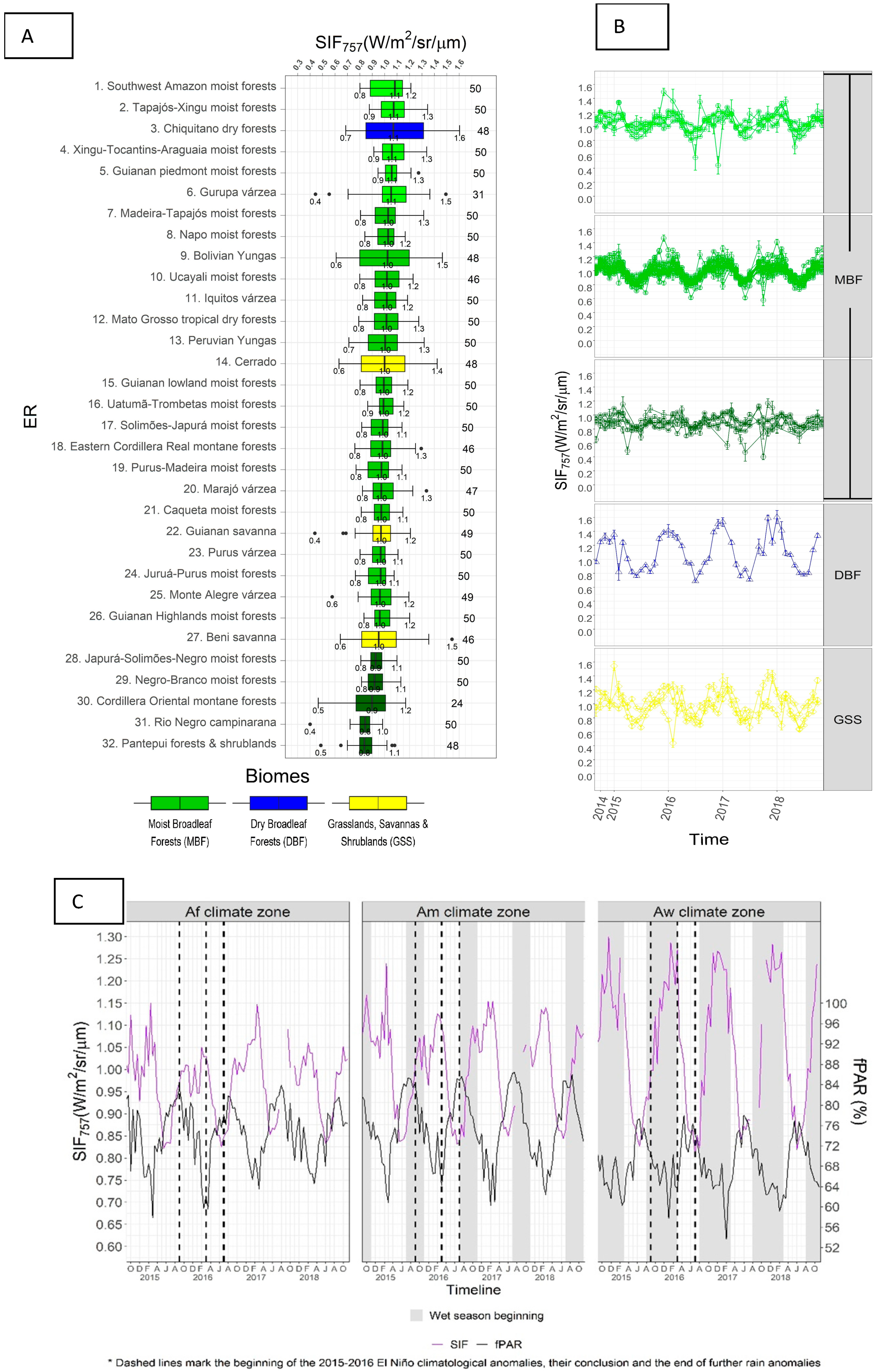
3.1. SIF₇₅₇ Phenological Diversity across ER and Climate Zones

The SIF₇₅₇ across ERs showed different spatial (Figure 2A) and temporal (Figure 2B) dynamics over the period from September 2014 to December 2018. We find subtle differences in SIF₇₅₇ phenology across different forest regions. MBF-ER (green values in Figure 2A) showed the highest SIF₇₅₇ values, but we also found that the SIF₇₅₇ from the DBF and GSS biomes was equal to or higher than that of the MBF-ER on reiterated occasions. We acknowledge that this SIF₇₅₇ variability, particularly that from GSS and DBF ER, may arise from natural or disturbed grasslands type vegetation, which we could not differentiate in the scope of our study. Moreover, we found a relatively higher temporal variability in the ERs close to the Andes (ERs 13 and 30), in those in the south and south-west (ER 9 and 18), and in those neighboring the non-MBF ERs, where forest cover is uncommon (Figure S2).

Although we did not determine the dry or the wet season for each ER, we observed a yearly phenological variation that resembles that of the climate zones in most ERs (Figure 2B), except for those with <0.95 W/m²/sr/μm. These MBF-ER-SIFs remain relatively stable throughout the year compared to all other ER-SIFs from the MBF biome.

The MBF-ERs cover approximately 5.2 million km² (~ 87% of the Amazon basin) and five of these ERs are some of the most productive regions, with a monthly median SIF₇₅₇ of more than 1.05 W/m²/sr/μm (ER 1, 2, 4, 5, and 6; ~1.3 million km²). The gradient of the SIF₇₅₇ medians across the ERs (Figure 2A) indicates that the first five ERs, with a monthly median >1.05 W/m²/sr/μm, may have a relatively higher contribution to SIF₇₅₇ within the basin. Among the 32 ERs under analysis, only 13 ERs reached or exceeded a monthly median of 1.25 W/m²/sr/μm (ER 2, 3, 4, 5, 6, 7, 9, 12, 13, 14, 18, 20, and 28; ~2.6 million km²). Five presented a notably wider interquartile range (≥0.24 W/m²/sr/μm), indicating a stronger seasonality (ER 1, 4, 7, 15, 26; ~1.7 million km²).

3.2. SIF₇₅₇ and fPAR Dynamics at Climate Scale

About 5.6 million km² of the Amazon basin is located within the Af, Am, and Aw KG-climate zones. The temporal SIF₇₅₇ and fPAR dynamics for these three KG-climate zones show direct temporal mismatches with each other (Figure 2C). We could not observe a relationship between the inter-yearly annual peaks in SIF₇₅₇ and the inter-yearly fPAR dynamics.

We found that SIF₇₅₇ decreases within the first-half of the year and increases during the second-half of the year. Furthermore, we observed a bi-yearly alternation in the SIF₇₅₇ peaks between December and March in the Af KG-climate zone. There, we also observed increases in the yearly minimum fPAR through the years, while it remained relatively constant at the Am climate zone. In addition, the Am KG-climate zone presented a constant decrease in the yearly minimum fPAR between 2014 and 2017. We also found that the cumulative SIF₇₅₇ at a climate scale follows the relation Af < Am < Aw. However, the coverage of their areas presents an opposite relationship, with 37%, 30%, and 27%, respectively.

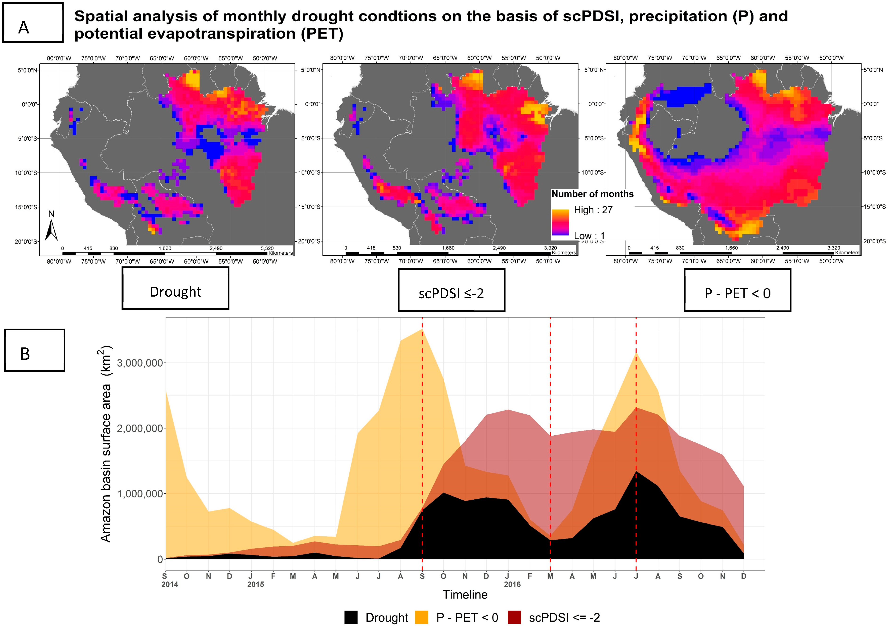
3.3. Drought Extent and Development

Drought conditions occurred predominantly in the north-eastern part of the Amazon basin (Figure 3A; ER 5, 15, 22, and 26; maximums >13 and ≤21 drought months/pixel (DMP)), ER 32 (maximum ≤ 15 DMP), ER 12 and 4 (maximum ≤ 9 DMP), and ER 19 and 31 (maximum ≤ 7 DMP), while the other ER pixels had six or fewer maximum DMP. The drought occurred in two waves between August 2015 and November 2016, with the second wave starting in April 2016 (Figure 3B).

The scPDSI indicated an anomalous water balance, which started in August 2015, reaching its first peak in October 2016. The drought conditions remained until January 2016 and decreased by March 2016. Then, a second wave of anomalous water balance conditions began in August 2016, peaked in July 2016, and decreased until December 2016. We did not find any pixel with PET < 0 or drought conditions at the western hemisphere of the Af KG-climate zone.

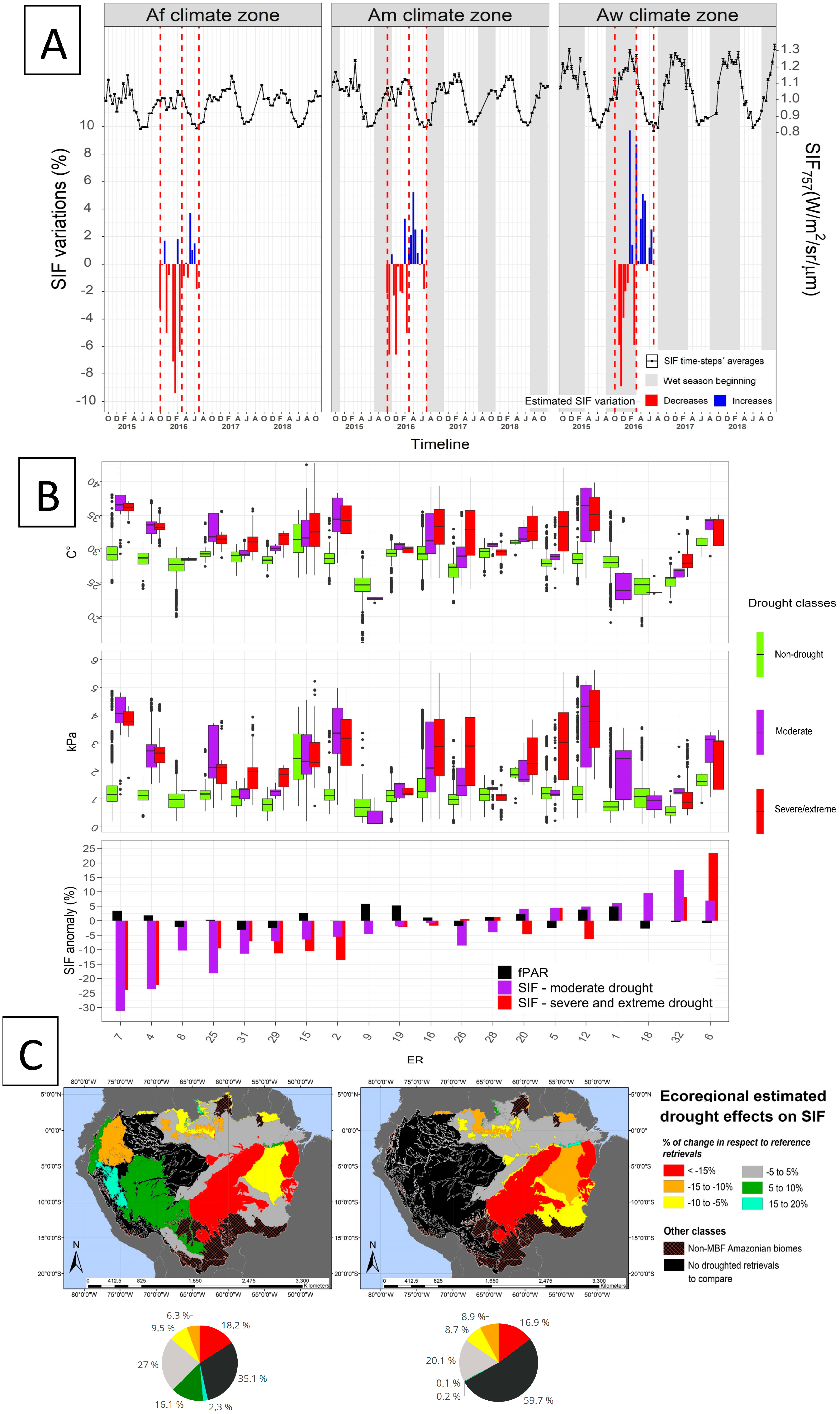
3.4. SIF₇₅₇ Response during the 2015/2016 El Niño Drought Event

We found different drought effects across the Amazonian MBF-ER in the Amazon basin during the El Niño 2015–2016 peak (Figure 4A,B; Appendix A

Table A2. Data from the drought effect estimation (Figure 4B,C in the main text) aggregated by ecoregions with scPDSI area sub-classes. In the table, for each ecoregion, information can be found on the ecoregion surface area within the Amazon river basin (km²), the SIF number of the retrievals for each scPDSI sub-class presented as per-mil of the total (1‰ = 130.4 retrievals), and the means for each scPDSI sub-class (W/m²/sr/um). The sampling extended from 01 October to 31 March for the time-frame of September 2014–December 2016.

Ecoregion		Quantity of SIF Samples (‰ over Total SIF Retrievals)/Mean SIF Value (W/m2/sr/um)			% of Change in SIF in Respect to Non-Drought
	Ecoregional Area (km2) within the Amazon Basin	Drought Classes			Moderate/Severe and Extreme-Drought Areas
		Non-Drought	Moderate	Severe/Extreme
1. Southwest Amazon moist forests	746,572	106.62/1.09	0.36/1.15	-/-	5.98/-
2. Tapajós–Xingu moist forests	335,000	40.99/1.15	5.87/1.09	9.09/1.00	−5.45/−13.43
4. Xingu-Tocantins–Araguaia moist forests	165,107	12.15/1.23	1.08/0.94	4.83/0.96	−23.64/−22.15
5. Guianan piedmont moist forests	88,536	29.8/1.04	3.06/1.08	24.85/1.08	4.45/4.45
6. Gurupa várzea	10,170	0.31/1.05	0.22/1.12	0.06/1.29	6.93/23.39
7. Madeira–Tapajós moist forests	716,661	78.25/1.09	1.87/0.75	1.7/0.83	−31.09/−23.90
8. Napo moist forests	250,652	64.57/1.09	1.02/0.98	-/-	−10.29/-
9. Bolivian Yungas	90,330	4.83/1.23	0.12/1.18	-/-	−4.54/-
10. Ucayali moist forests	114,259	6.16/1.12	0.01/1.57	-/-	39.76/-
11. Iquitos várzea	114,259	16.81/1.08	-/-	-/-	-/-
12. Mato Grosso tropical dry forests	306,884	8.06/1.10	0.92/1.15	1.97/1.03	4.83/−6.36
13. Peruvian Yungas	175,875	2.29/1.00	-/-	-/-	-/-
15. Guianan lowland moist forests	34,696	12.54/1.09	18.66/1.02	4.93/0.97	−6.47/−10.48
16. Uatumã–Trombetas moist forests	444,474	104.98/1.01	68.95/1.01	109.99/1.00	−0.73/−1.66
17. Solimões–Japurá moist forests	166,902	7.75/1.05	-/-	-/-	-/-
18. Eastern Cordillera Real montane forests	81,955	13.69/1.08	0.18/1.18	-/-	9.58/-
19. Purus–Madeira moist forests	173,482	39.43/1.01	0.37/0.99	2.01/0.99	−1.98/−2.15
20. Marajó várzea	40,080	0.87/1.00	0.54/1.04	4.07/0.95	4.12/−4.67
21. Caqueta moist forests	168,098	0.08/1.02	-/-	-/-	-/-
23. Purus várzea	176,473	12.13/0.98	-/-	-/-	-/-
24. Juruá–Purus moist forests	241,679	19.19/1.02	-/-	-/-	-/-
25. Monte Alegre várzea	66,402	7.03/1.06	0.53/0.87	1.05/0.96	−18.21/−9.51
26. Guianan Highlands moist forests	34,098	10.09/1.00	2.03/0.92	5.23/1.01	−8.57/0.62
28. Japurá–Solimões-Negro moist forests	267,402	52.73/0.99	3.83/0.95	6.49/1.00	−3.97/1.27
29. Negro–Branco moist forests	93,322	29.63/0.95	0.69/0.88	4.11/0.84	−7.01/−11.25
31. Rio Negro campinarana	80,759	15.46/0.87	1.33/0.77	3.59/0.81	−11.39/−7.13
32. Pantepui forests and shrublands	6580	4.01/0.84	0.41/0.99	3.52/0.91	17.56/8.16
Total SIF retrievals in this experiment: 130,413

). The drought indicator clearly captured an increased VPD and increased temperature values across the KG zones and ER. Our analysis of the SIF₇₅₇ variations during the CARA period in the Af, Am, and Aw climate zones showed a net change of −2.42%, −1.46%, and −1.42%, respectively (Figure 4A). For the ER, we estimated that the drought effects varied from −31.09% (ER 7) to +17.56% (ER 32) during the El Niño 2015–2016 drought peak. We assessed 21 MBF-ER and found that 8 ER showed a decrease in SIF₇₅₇ below −5% under moderate and severe/extreme drought conditions (Figure 4B; ER 2, 4, 7, 8, 15, 25, 29, 31), although the fPAR increased in four of these cases (ER 7, 4, 25, and 15). Drought areas yielded SIF₇₅₇ increases above 5% at 4 ER (1, 18, 32, and 6). We found an increased IQR for the temperature values in all ERs except for ER 9 and 18. Moreover, we also observed increases in the VPD in all ERs under drought except for ER 15, 9, 5, and 18.

The overall results indicate that the largest net MBF-SIF₇₅₇ change occurred in the Af climate zone. However, the analysis that also considered drought sub-regions indicated that the most notable SIF₇₅₇ decreases in vegetation occurred in the Am and Aw climate zones (Figure S3). Moreover, a higher spread of the time-step means was observed in the Am and Aw climate zones under moderate and severe/extreme drought than that under non-drought conditions compared to Af.

Figure 4C shows a drought vulnerability map across the Amazonian vegetation ecosystems including their SIF₇₅₇ values. All values used for the drought-peak estimation, the number of retrievals, and the area of each ER are presented in Appendix A Table A2. The drought effects on SIF₇₅₇ could not be quantified due to the absence of moderate, or severe and extreme droughted retrievals at ERs 11, 13, 17, 21, 23, and 24 (the black areas in Figure 4C).

4. Discussion

4.1. Phenological Diversity of SIF₇₅₇

The subtle intra-biome differences in monthly SIF₇₅₇ patterns across the MBF-ER (Figure 2A,B) suggest that there is an SIF phenological diversity that is finer in spatial resolution than the currently applied resolution of climate zones for assessing SIF (such as [7,29]). These phenological differences are evident between the ERs of different biomes and have been analyzed beyond the extent of the Amazon basin in Brazil [30]. The KG-climate zones combine the SIF values of areas from different biomes. Such an approach merges the SIF from plant communities with the different main CO₂ fixation pathways (e.g., the C₄ from the GSS with C₃ and CAM from the MBF), particularly in the Am and Aw climate zones. Aggregation on this basis may mislead SIF interpretations for ${\mathsf{\Phi }}_F$, which differs considerably across plants with different CO₂ fixation pathways [15].

Similarly to the previous research on Amazonian vegetation SIF phenology [29], we showed that photosynthetic activity during the dry season is lower than during the wet season. SIF₇₅₇ variability at the level of KG-climate zones can be attributed to the beginning of the wet season in our study (i.e., the beginning of the wet season shown in Figure 2A). The phenological variations in Figure 2B have distinctive yearly minimums and maximums which allow one to coarsely characterize each ER-SIF´s signature. Hence, our research findings confirm the great potential of OCO-2 in capturing the inter-biome temporal variability in the SIFs of different South American biome vegetation types [30].

4.2. SIF₇₅₇ and fPAR Dynamics at the Scale of Climate Zones

In our study, fPAR and SIF₇₅₇ showed a temporal mismatch (Figure 2C), which suggests that the fluorescence quantum yield in the band of measurement (${\mathsf{\Phi }}_F$) and the probability that photons can escape the canopy (${\Omega }_C$) play an important role in the SIF of plants compared to fPAR. SIF-fPAR temporal mismatches were found in 2015 [13], where the land surface temperature (proxy for PAR) and nadir BRDF (bidirectional reflectance distribution function) adjusted reflectance (NBAR) in the near-infrared band of the MODIS satellite (an fPAR proxy) showed a temporal mismatch with GOSAT SIF across the climate zones in Amazonia. We agree with the implications of previous findings on the seasonality of SIF in the Amazon [13], which showed that there is leaf phenological diversity [63] that cannot be captured at the scale of KG-climate zones [7,29] and biomes [30,44]. Thus, it may be valid to aggregate SIF time-series of retrievals over combined classes of ERs to capture SIF dynamics and magnitude differences. This is because ERs are based on biomes maps considering the vegetation´s climatological and ecological dimensions (Table 1) that the OCO-2 captures in terms of ${\mathsf{\Phi }}_F$ and ${\Omega }_C$ [9,19].

The reason behind the inverse relation observed between SIF₇₅₇ and the fPAR may be related to the structural effects at canopy level that the seasonal increase in leaf growth [63] can have on ${\Omega }_C$ and fPAR. Research has been done on fitting the parameters of SIF₇₆₀ with reflectance between 400 and 900 nm from the canopy of crop systems in a SCOPE (Soil Canopy Observation, Photochemistry and Energy Fluxes) model [64]. They found that the reflectance properties alone fit well with the SIF in the model, while simulations including a control of ${\mathsf{\Phi }}_F$ according to the maximum rate of the carboxylation parameter performed marginally better. These results support the argument that SIF might be strongly determined by canopy structure, and thus ${\Omega }_C$, and not as much by canopy biochemistry (i.e., ${\mathsf{\Phi }}_F$) [9].

Interestingly, canopies with similar fPAR can emit different levels of SIF and have different levels of GPP [65]. It has been reported that structural parameters, such as near-infrared reflectance (NIRv), correlate better with canopy GPP than does fPAR [65] because higher NIRv (as well as more SIF) corresponds to a larger fraction of sun leaves [65], which gives them a higher maximum rate of carboxylation than shade leaves. Thus, it is possible that SIF seasonality may be better explained by forest structural factors that determine the fraction of sun and shade leaves than with fPAR.

4.3. Drought Definition for Assessing SIF Variation during Drought

We applied the scPDSI to define drought, which, in contrast to other drought indicators (e.g., CWD, SPI, or SPEI), considers soil characteristics and models water fluxes as runoff or recharge, along with common water balance drivers, such as precipitation, temperature, and evapotranspiration. Our drought definition excluded a considerable area of the western Amazon basin region which did not experience scPDSI ≤ −2 or P – PET < 0 conditions.

When defining drought at a spatio–temporal scale comparable to that of OCO-2 SIF, the main source of uncertainty is the lack of long-term observational data on common water balance drivers [66] and the absence of in-depth high-resolution soil descriptors in UN-FAO maps [58]. Unless the Amazonian measurement station network is upgraded to provide the scientific community with better quality data, the responses of the Amazon rainforest´s vegetation to climate change at an ER scale will have to be analyzed and forecasted using other climatological datasets (e.g., ERA-5 from the European Centre for Medium-Range Weather Forecasts [67]) and soil maps [68] in addition to those analyzed here.

4.4. SIF₇₅₇ Response during the El Niño 2015–2016 Extreme Drought Event

Although it was proven with plant-level measurements of active fluorescence that, under controlled environments, the carbon-assimilation of plant species responds differently to drought [69,70,71], only few studies have explored the changes in SIF₇₅₇ during the drought in the Amazonia (e.g., [7]). We showed that the MBF in the Af KG-climate zone had the highest net SIF₇₅₇ decreases compared to the Am and Aw KG-climate zones during the CARA period (Figure 4A). This contrasts with the lowest VPD (higher humidity) in the Af compared to Am and Aw (Figure S3) and demonstrates that the Af environment is more humid, but its vegetation’s SIF₇₅₇ is more sensitive to variations in the water balance.

The estimated drought-driven SIF₇₅₇ changes across the ERs (Figure 4B) may be indicators of the changes in GPP dynamics between different drought categories of the same ER. These may also be indicators of mortality [71] of hydraulically vulnerable species [26] that would lead to variations in GPP. Such GPP variations have been reported to have enormous impacts on the structure and function of the Amazonian forest ecosystems [72,73], as well as on their provisioning of ecosystem services [74,75]. However, it is difficult to tell when a plant that contributes with chlorophyll fluorescence radiance to a SIF retrieval is dead [76] and, as a consequence, its ecological niche has been occupied by better adapted species [24,25,26], or when physiological responses have taken place. This is because an OCO-2 SIF retrieval captures a unit of land with a diverse plant community under constant interaction.

If physiological responses are taking place at the plant level, one can expect a reduced photosynthesis [63]. However, at the community level, we observed positive and negative ER-SIF₇₅₇ variations. We hypothesize that the variations could also be related to drought-driven ecological dynamics with potential for compelling the ERs’ community demography to express a higher or lower ${\mathsf{\Phi }}_F$ and ${\Omega }_C$ (e.g., the proliferation of tropical plants that increase tree mortality [27], a decrease in pollinators resulting in decreased natality of specific plant species [77], or a decrease in the fauna’s floristic resources, thereby affecting the fauna composition [78,79] and leading to changes in ${\mathsf{\Phi }}_F$ by limiting the plants’ N availability [16] from manure and urine stock flows). Nevertheless, similar to previous results [7], we found a widespread SIF₇₅₇ reduction during the El Niño 2015–2016 phenomena in which the positive and negative ER-SIF₇₅₇ variations suggest that both physiological responses and mortality may be taking place with a higher frequency in ERs with higher SIF₇₅₇ variations.

Our analysis also provides insights into the magnitude of VPD changes, their correlation with temperature across the Amazon region during the El Niño 2015–2016 extreme drought, and the related SIF response. Notably, the ERs experienced different VPD under drought, which may be related to whether they are able to decouple photosynthesis from transpiration during heat extremes [80].

The decrease in SIF in combination with increases in fPAR in drought areas has been linked to a higher heat dissipation of plants through non-photochemical quenching (NPQ; [81,82]). fPAR reflects the structure of vegetation, whereas SIF is influenced by structural (APAR and ${\Omega }_C$) and physiological (LUE and ${\mathsf{\Phi }}_F$) components. However, to physiologically consider the allocation of APAR in SIF, NPQ, or photochemistry, PAR measurements are required to calculate APAR. Together with ${\Omega }_C$, these measurements would allow one to remove the structural components of SIF and provide a proxy for NPQ. Nevertheless, we found large differences in temperature and VPD between drought and non-drought areas of the same ER (Figure 4B). In this case, the ER characterization of SIF under different drought classes (Appendix A Table A2) can help tracking changes in the behavior of the ERs by comparing their non-drought values over time with their droughted SIF values during the El Niño 2015–2016 anomaly period.

5. Conclusions

Here, we showed SIF₇₅₇ variability at an ER scale. The extent to which the vegetation communities’ ${\mathsf{\Phi }}_F$ and ${\Omega }_C$ influence the SIF retrievals still requires elucidation. The Amazon region is the most biodiverse place on Earth. Therefore, uncertainties about the extent to which there is linearity between SIF and GPP remain for this particular region. However, our study on ERs across the Amazon basin demonstrates that it is possible to differentiate high-resolution SIF responses, which are related to vital photosynthetic processes and carbon fixation. This approach, combined with further data on the factors related to SIF (${\mathsf{\Phi }}_F$ and ${\Omega }_C$), and the ER-SIF specific responses to drought in terms of the LUE-SIF-GPP relationships could help to provide more accurate methods to estimate the carbon stocks and flows with unprecedented spatial and temporal resolutions.

Finally, due to the extraordinarily high uncertainty about the association of SIF-GPP’s relationship to OCO-2 SIF and satellite-based GPP products in rainforests and in South America, the next step would be to compare pertinent high-resolution air- or space-borne data with ground-based measurements, for example, data from eddy-flux towers or ground-based SIF instruments. Such data are difficult to acquire in the Amazon region, but might be relevant for comprehensively predicting GPP from the extremely biodiverse Amazonian ecosystems.

References

1. Saatchi, S.S.; Harris, N.L.; Brown, S.; Lefsky, M.; Mitchard, E.T.A.; Salas, W.; Zutta, B.R.; Buermann, W.; Lewis, S.L.; Hagen, S.; et al. Benchmark map of forest carbon stocks in tropical regions across three continents. Proc. Natl. Acad. Sci. USA 2011, 108, 9899–9904. [Google Scholar] [CrossRef] [PubMed] [Green Version]
2. Morley, R.J. Origin and Evolution of Tropical Rain Forests; Wiley: Chichester, UK, 2000. [Google Scholar]
3. Pan, Y.; Birdsey, R.A.; Fang, J.; Houghton, R.; Kauppi, P.E.; Kurz, W.A.; Phillips, O.L.; Shvidenko, A.; Lewis, S.L.; Canadell, J.G.; et al. A large and persistent carbon sink in the world’s forests. Science 2011, 333, 988–993. [Google Scholar] [CrossRef] [Green Version]
4. Jiménez-Muñoz, J.C.; Mattar, C.; Barichivich, J.; Santamaría-Artigas, A.; Takahashi, K.; Malhi, Y.; Sobrino, J.A.; van der Schrier, G. Record-breaking warming and extreme drought in the Amazon rainforest during the course of El Niño 2015–2016. Sci. Rep. 2016, 6, 33130. [Google Scholar] [CrossRef] [PubMed] [Green Version]
5. Lewis, S.L.; Brando, P.M.; Phillips, O.L.; van der Heijden, G.M.F.; Nepstad, D. The 2010 Amazon drought. Science 2011, 331, 554. [Google Scholar] [CrossRef] [PubMed]
6. Phillips, O.L.; Aragão, L.E.O.C.; Lewis, S.L.; Fisher, J.B.; Lloyd, J.; López-González, G.; Malhi, Y.; Monteagudo, A.; Peacock, J.; Quesada, C.A.; et al. Drought sensitivity of the Amazon rainforest. Science 2009, 323, 1344–1347. [Google Scholar] [CrossRef] [PubMed] [Green Version]
7. Koren, G.; van Schaik, E.; Araújo, A.C.; Boersma, K.F.; Gärtner, A.; Killaars, L.; Kooreman, M.L.; Kruijt, B.; van der Laan-Luijkx, I.T.; von Randow, C.; et al. Widespread reduction in sun-induced fluorescence from the Amazon during the 2015/2016 El Niño. Philos. Trans. R. Soc. B Biol. Sci. 2018, 373, 20170408. [Google Scholar] [CrossRef]
8. Brienen, R.J.W.; Phillips, O.L.; Feldpausch, T.R.; Gloor, E.; Baker, T.R.; Lloyd, J.; Lopez-Gonzalez, G.; Monteagudo-Mendoza, A.; Malhi, Y.; Lewis, S.L.; et al. Long-term decline of the Amazon carbon sink. Nature 2015, 519, 344. [Google Scholar] [CrossRef] [Green Version]
9. Frankenberg, C.; Berry, J. Solar induced chlorophyll fluorescence: Origins, relation to photosynthesis and retrieval. In Comprehensive Remote Sensing; Elsevier: Amsterdam, The Netherlands, 2018; pp. 143–162. [Google Scholar]
10. Parazoo, N.C.; Bowman, K.; Fisher, J.B.; Frankenberg, C.; Jones, D.B.A.; Cescatti, A.; Pérez-Priego, O.; Wohlfahrt, G.; Montagnani, L. Terrestrial gross primary production inferred from satellite fluorescence and vegetation models. Glob. Chang. Biol. 2014, 20, 3103–3121. [Google Scholar] [CrossRef]
11. MacBean, N.; Maignan, F.; Bacour, C.; Lewis, P.; Peylin, P.; Guanter, L.; Köhler, P.; Gómez-Dans, J.; Disney, M. Strong constraint on modelled global carbon uptake using solar-induced chlorophyll fluorescence data. Sci. Rep. 2018, 8, 1973. [Google Scholar] [CrossRef]
12. Bertani, G.; Wagner, F.; Anderson, L.; Aragão, L. Chlorophyll fluorescence data reveals climate-related photosynthesis seasonality in Amazonian forests. Remote Sens. 2017, 9, 1275. [Google Scholar] [CrossRef] [Green Version]
13. Xu, L.; Saatchi, S.S.; Yang, Y.; Myneni, R.B.; Frankenberg, C.; Chowdhury, D.; Bi, J. Satellite observation of tropical forest seasonality: Spatial patterns of carbon exchange in Amazonia. Environ. Res. Lett. 2015, 10, 84005. [Google Scholar] [CrossRef]
14. Li, X.; Xiao, J.; He, B. Chlorophyll fluorescence observed by OCO-2 is strongly related to gross primary productivity estimated from flux towers in temperate forests. Remote Sens. Environ. 2018, 204, 659–671. [Google Scholar] [CrossRef]
15. Björkman, O.; Demmig, B. Photon yield of O2 evolution and chlorophyll fluorescence characteristics at 77 K among vascular plants of diverse origins. Planta 1987, 170, 489–504. [Google Scholar] [CrossRef]
16. Lin, Y.-C.; Hu, Y.-G.; Ren, C.-Z.; Guo, L.-C.; Wang, C.-L.; Jiang, Y.; Wang, X.-J.; Phendukani, H.; Zeng, Z.-H. Effects of nitrogen application on chlorophyll fluorescence parameters and leaf gas exchange in naked oat. J. Integr. Agric. 2013, 12, 2164–2171. [Google Scholar] [CrossRef] [Green Version]
17. Wu, G.; Liu, H.; Hua, L.; Luo, Q.; Lin, Y.; He, P.; Feng, S.; Liu, J.; Ye, Q. Differential responses of stomata and photosynthesis to elevated temperature in two co-occurring subtropical forest tree species. Front. Plant Sci. 2018, 9, 467. [Google Scholar] [CrossRef] [PubMed] [Green Version]
18. Coops, N.C.; Hilker, T.; Hall, F.G.; Nichol, C.J.; Drolet, G.G. Estimation of light-use efficiency of terrestrial ecosystems from space: A status report. Bioscience 2010, 60, 788–797. [Google Scholar] [CrossRef] [Green Version]
19. Sun, Y.; Fu, R.; Dickinson, R.; Joiner, J.; Frankenberg, C.; Gu, L.; Xia, Y.; Fernando, N. Drought onset mechanisms revealed by satellite solar-induced chlorophyll fluorescence: Insights from two contrasting extreme events. J. Geophys. Res. 2015, 120, 2427–2440. [Google Scholar] [CrossRef]
20. Sun, Y.; Frankenberg, C.; Wood, J.D.; Schimel, D.S.; Jung, M.; Guanter, L.; Drewry, D.T.; Verma, M.; Porcar-Castell, A.; Griffis, T.J.; et al. OCO-2 advances photosynthesis observation from space via solar-induced chlorophyll fluorescence. Science 2017, 358. [Google Scholar] [CrossRef] [Green Version]
21. Keenan, T.; Sabate, S.; Gracia, C. The importance of mesophyll conductance in regulating forest ecosystem productivity during drought periods. Glob. Chang. Biol. 2010, 16, 1019–1034. [Google Scholar] [CrossRef]
22. Bréda, N.; Huc, R.; Granier, A.; Dreyer, E. Temperate forest trees and stands under severe drought: A review of ecophysiological responses, adaptation processes and long-term consequences. Ann. Sci. 2006, 63, 625–644. [Google Scholar] [CrossRef] [Green Version]
23. Mencuccini, M.; Minunno, F.; Salmon, Y.; Martínez-Vilalta, J.; Hölttä, T. Coordination of physiological traits involved in drought-induced mortality of woody plants. New Phytol. 2015, 208, 396–409. [Google Scholar] [CrossRef] [PubMed] [Green Version]
24. Bilton, M.C.; Metz, J.; Tielbörger, K. Climatic niche groups: A novel application of a common assumption predicting plant community response to climate change. Perspect. Plant Ecol. Evol. Syst. 2016, 19, 61–69. [Google Scholar] [CrossRef] [Green Version]
25. Gitlin, A.R.; Sthultz, C.M.; Bowker, M.A.; Stumpf, S.; Paxton, K.L.; Kennedy, K.; Muñoz, A.; Bailey, J.K.; Whitham, T.G. Mortality gradients within and among dominant plant populations as barometers of ecosystem change during extreme drought. Conserv. Biol. 2006, 20, 1477–1486. [Google Scholar] [CrossRef] [PubMed]
26. Powers, J.S.; Vargas, G.G.; Brodribb, T.J.; Schwartz, N.B.; Perez-Aviles, D.; Smith-Martin, C.M.; Becknell, J.M.; Aureli, F.; Blanco, R.; Calderón-Morales, E.; et al. A catastrophic tropical drought kills hydraulically vulnerable tree species. Glob. Chang. Biol. 2020. [Google Scholar] [CrossRef]
27. Umaña, M.N.; Forero-Montaña, J.; Nytch, C.J.; Thompson, J.; Uriarte, M.; Zimmerman, J.; Swenson, N.G. Dry conditions and disturbance promote liana seedling survival and abundance. Ecology 2019, 100, e02556. [Google Scholar] [CrossRef] [Green Version]
28. Guanter, L.; Frankenberg, C.; Dudhia, A.; Lewis, P.E.; Gómez-Dans, J.; Kuze, A.; Suto, H.; Grainger, R.G. Retrieval and global assessment of terrestrial chlorophyll fluorescence from GOSAT space measurements. Remote Sens. Environ. 2012, 121, 236–251. [Google Scholar] [CrossRef]
29. Lee, J.-E.; Frankenberg, C.; van der Tol, C.; Berry, J.A.; Guanter, L.; Boyce, C.K.; Fisher, J.B.; Morrow, E.; Worden, J.R.; Asefi, S.; et al. Forest productivity and water stress in Amazonia: Observations from GOSAT chlorophyll fluorescence. Proc. Biol. Sci. 2013, 280, 20130171. [Google Scholar] [CrossRef] [Green Version]
30. Merrick, T.; Pau, S.; Jorge, M.L.S.P.; Bennartz, R.; Silva, T.S.F. Spatiotemporal patterns and phenology of tropical vegetation solar-induced chlorophyll fluorescence across Brazilian biomes using satellite observations. Remote Sens. 2019, 11, 1746. [Google Scholar] [CrossRef] [Green Version]
31. Wunch, D.; Wennberg, P.O.; Toon, G.C.; Connor, B.J.; Fisher, B.; Osterman, G.B.; Frankenberg, C.; Mandrake, L.; O’Dell, C.; Ahonen, P.; et al. A method for evaluating bias in global measurements of CO2 total columns from space. Atmos. Chem. Phys. 2011, 11, 12317–12337. [Google Scholar] [CrossRef] [Green Version]
32. Wunch, D.; Toon, G.C.; Blavier, J.-F.L.; Washenfelder, R.A.; Notholt, J.; Connor, B.J.; Griffith, D.W.T.; Sherlock, V.; Wennberg, P.O. The total carbon column observing network. Philos. Trans. A Math. Phys. Eng. Sci. 2011, 369, 2087–2112. [Google Scholar] [CrossRef] [Green Version]
33. O’Dell, C.W.; Connor, B.; Bösch, H.; Brien, D.; Frankenberg, C.; Castano, R.; Christi, M.; Eldering, D.; Fisher, B.; Gunson, M.; et al. The ACOS CO2 retrieval algorithm—Part 1: Description and validation against synthetic observations. Atmos. Meas. Tech. 2012, 5, 99–121. [Google Scholar]
34. Crisp, D.; Fisher, B.M.; O’Dell, C.; Frankenberg, C.; Basilio, R.; Bösch, H.; Brown, L.R.; Castano, R.; Connor, B.; Deutscher, N.M.; et al. The ACOS CO2 retrieval algorithm—Part II: Global X CO2 data characterization. Atmos. Meas. Tech. 2012, 5, 687–707. [Google Scholar] [CrossRef] [Green Version]
35. Frankenberg, C.; Pollock, R.; Lee, R.A.M.; Rosenberg, R.; Blavier, J.-F.; Crisp, D.; O’Dell, C.W.; Osterman, G.B.; Roehl, C.; Wennberg, P.O.; et al. The orbiting carbon observatory (OCO-2): Spectrometer performance evaluation using pre-launch direct sun measurements. Atmos. Meas. Tech. Discuss. 2014, 7, 7641–7670. [Google Scholar] [CrossRef]
36. Frankenberg, C.; O’Dell, C.; Berry, J.; Guanter, L.; Joiner, J. Prospects for chlorophyll fluorescence remote sensing from the orbiting carbon observatory-2. Remote Sens. Environ. 2014, 147, 1–12. [Google Scholar] [CrossRef] [Green Version]
37. Bhattacharjee, S.; Chen, J. Prediction of Satellite-based Column CO2 Concentration by Combining Emission Inventory and LULC information. IEEE Trans. Geosci. Remote Sens. 2020. [Google Scholar] [CrossRef]
38. Köhler, P.; Frankenberg, C.; Magney, T.S. Global retrievals of solar-induced chlorophyll fluorescence with TROPOMI: First results and intersensor comparison to OCO-2. AGU Adv. Earth Space Sci. 2018. [Google Scholar] [CrossRef] [Green Version]
39. Frankenberg, C.; Fisher, J.B.; Worden, J.; Badgley, G.; Saatchi, S.S.; Lee, J.-E.; Toon, G.C.; Butz, A.; Jung, M.; Kuze, A.; et al. New global observations of the terrestrial carbon cycle from GOSAT: Patterns of plant fluorescence with gross primary productivity. Geophys. Res. Lett. 2011, 38. [Google Scholar] [CrossRef] [Green Version]
40. Joiner, J.; Guanter, L.; Lindstrot, R.; Voigt, M.; Vasilkov, A.P.; Middleton, E.M.; Huemmrich, K.F.; Yoshida, Y.; Frankenberg, C. Global monitoring of terrestrial chlorophyll fluorescence from moderate-spectral-resolution near-infrared satellite measurements: Methodology, simulations, and application to GOME-2. Atmos. Meas. Tech. 2013, 6, 2803–2823. [Google Scholar] [CrossRef] [Green Version]
41. Sun, Y.; Frankenberg, C.; Jung, M.; Joiner, J.; Guanter, L.; Köhler, P.; Magney, T. Overview of Solar-Induced chlorophyll Fluorescence (SIF) from the Orbiting Carbon Observatory-2: Retrieval, cross-mission comparison, and global monitoring for GPP. Remote Sens. Environ. 2018, 209, 808–823. [Google Scholar] [CrossRef]
42. Olson, D.M.; Dinerstein, E.; Wikramanayake, E.D.; Burgess, N.D.; Powell, G.V.N.; Underwood, E.C.; D’Amico, J.A.; Itoua, I.; Strand, H.E.; Morrison, J.C.; et al. Terrestrial ecoregions of the world: A new map of life on earth. Bioscience 2001, 51, 933. [Google Scholar] [CrossRef]
43. Dinerstein, E.; Olson, D.M.; Graham, D.J.; Webster, A.L.; Primm, S.A.; Bookbinder, M.P.; Ledec, G. A Conservation Assessment of the Terrestrial Ecoregions of Latin America and the Caribbean; World Bank: Washington, DC, USA, 1995. [Google Scholar]
44. Li, X.; Xiao, J.; He, B.; Altaf Arain, M.; Beringer, J.; Desai, A.R.; Emmel, C.; Hollinger, D.Y.; Krasnova, A.; Mammarella, I.; et al. Solar-induced chlorophyll fluorescence is strongly correlated with terrestrial photosynthesis for a wide variety of biomes: First global analysis based on OCO-2 and flux tower observations. Glob. Chang. Biol. 2018. [Google Scholar] [CrossRef] [PubMed]
45. Mayorga, E.; Logsdon, M.G.; Ballester, M.V.R.; Richey, J.E. LBA-ECO CD-06 Amazon river basin land and stream drainage direction maps. ORNL DAAC 2012. [Google Scholar] [CrossRef]
46. Dinerstein, E.; Olson, D.; Joshi, A.; Vynne, C.; Burgess, N.D.; Wikramanayake, E.; Hahn, N.; Palminteri, S.; Hedao, P.; Noss, R.; et al. An ecoregion-based approach to protecting half the terrestrial realm. Bioscience 2017, 67, 534–545. [Google Scholar] [CrossRef] [PubMed]
47. Kottek, M.; Grieser, J.; Beck, C.; Rudolf, B.; Rubel, F. World map of the Köppen-Geiger climate classification updated. METZ 2006, 15, 259–263. [Google Scholar] [CrossRef]
48. Frankenberg, C. Solar Induced Chlorophyll Fluorescence: OCO-2 Lite Files (B7000) User Guide. Available online: https://docserver.gesdisc.eosdis.nasa.gov/public/project/OCO/OCO2_SIF_B7000_Product_Description_090215.pdf (accessed on 14 January 2020).
49. NASA. OCO2 Data Portal. Available online: https://co2.jpl.nasa.gov/#mission=OCO-2 (accessed on 3 October 2019).
50. Eldering, A.; Wennberg, P.O.; Crisp, D.; Schimel, D.S.; Gunson, M.R.; Chatterjee, A.; Liu, J.; Schwandner, F.M.; Sun, Y.; O’Dell, C.W.; et al. The orbiting carbon observatory-2 early science investigations of regional carbon dioxide fluxes. Science 2017, 358. [Google Scholar] [CrossRef] [Green Version]
51. Goulas, Y.; Daumard, F.; Ounis, A.; Rhoul, C.; Lopez, M.L.; Moya, I. Monitoring the diurnal time course of vegetation dynamics with geostationary observations: The GFLEX project. In Proceedings of the 6th Workshop on Hyperspectral Image and Signal Processing: Evolution in Remote Sensing (WHISPERS), Lausanne, Switzerland, 24–27 June 2014; pp. 1–4. [Google Scholar]
52. Hansen, M.C.; Potapov, P.V.; Moore, R.; Hancher, M.; Turubanova, S.A.A.; Tyukavina, A.; Thau, D.; Stehman, S.V.; Goetz, S.J.; Loveland, T.R. High-resolution global maps of 21st-century forest cover change. Science 2013, 342, 850–853. [Google Scholar] [CrossRef] [Green Version]
53. Wells, N.; Goddard, S.; Hayes, M.J. A self-calibrating palmer drought severity index. J. Clim. 2004, 17, 2335–2351. [Google Scholar] [CrossRef]
54. Dai, A.; Trenberth, K.E.; Qian, T. A global dataset of palmer drought severity index for 1870–2002: Relationship with soil moisture and effects of surface warming. J. Hydrometeorol. 2004, 5, 1117–1130. [Google Scholar] [CrossRef]
55. Van der Schrier, G.; Barichivich, J.; Briffa, K.R.; Jones, P.D. A scPDSI-based global data set of dry and wet spells for 1901–2009. J. Geophys. Res. Atmos. 2013, 118, 4025–4048. [Google Scholar] [CrossRef]
56. Zang, C.S.; Buras, A.; Esquivel-Muelbert, A.; Jump, A.S.; Rigling, A.; Rammig, A. Standardized drought indices in ecological research: Why one size does not fit all. Glob. Chang. Biol. 2019. [Google Scholar] [CrossRef] [Green Version]
57. Dee, D.P.; Uppala, S.M.; Simmons, A.J.; Berrisford, P.; Poli, P.; Kobayashi, S.; Andrae, U.; Balmaseda, M.A.; Balsamo, G.; Bauer, P.; et al. The ERA-Interim reanalysis: Configuration and performance of the data assimilation system. Q. J. R. Meteorol. Soc. 2011, 137, 553–597. [Google Scholar] [CrossRef]
58. Food and Agriculture Organization of the United Nations. Digital Soil Map of the World and Derived Soil Properties; FAO: Rome, Italy, 2003. [Google Scholar]
59. Şen, Z. Applied Drought Modeling, Prediction, and Mitigation; Elsevier: Amsterdam, The Netherlands, 2015. [Google Scholar]
60. Yan, K.; Park, T.; Yan, G.; Chen, C.; Yang, B.; Liu, Z.; Nemani, R.; Knyazikhin, Y.; Myneni, R. Evaluation of MODIS LAI/FPAR product collection 6. Part 1: Consistency and improvements. Remote Sens. 2016, 8, 359. [Google Scholar] [CrossRef] [Green Version]
61. Yan, K.; Park, T.; Yan, G.; Liu, Z.; Yang, B.; Chen, C.; Nemani, R.; Knyazikhin, Y.; Myneni, R. Evaluation of MODIS LAI/FPAR product collection 6. Part 2: Validation and intercomparison. Remote Sens. 2016, 8, 460. [Google Scholar] [CrossRef] [Green Version]
62. Huffman, G.J.; Bolvin, D.T.; Nelkin, E.J.; Wolff, D.B.; Adler, R.F.; Gu, G.; Hong, Y.; Bowman, K.P.; Stocker, E.F. The TRMM multisatellite precipitation analysis (TMPA): Quasi-global, multiyear, combined-sensor precipitation estimates at fine scales. J. Hydrometeor. 2007, 8, 38–55. [Google Scholar] [CrossRef]
63. Wu, J.; Albert, L.P.; Lopes, A.P.; Restrepo-Coupe, N.; Hayek, M.; Wiedemann, K.T.; Guan, K.; Stark, S.C.; Christoffersen, B.; Prohaska, N.; et al. Leaf development and demography explain photosynthetic seasonality in Amazon evergreen forests. Science 2016, 351, 972–976. [Google Scholar] [CrossRef] [Green Version]
64. Van der Tol, C.; Rossini, M.; Cogliati, S.; Verhoef, W.; Colombo, R.; Rascher, U.; Mohammed, G. A model and measurement comparison of diurnal cycles of sun-induced chlorophyll fluorescence of crops. Remote Sens. Environ. 2016, 186, 663–677. [Google Scholar] [CrossRef]
65. Badgley, G.; Field, C.B.; Berry, J.A. Canopy near-infrared reflectance and terrestrial photosynthesis. Sci. Adv. 2017, 3, e1602244. [Google Scholar] [CrossRef] [Green Version]
66. Hans, H.; Dee, D.J.E.N. ERA5 reanalysis is in production. ECMWF Newsl. 2016, 147, 5–6. [Google Scholar]
67. Dijkshoorn, J.A.; van Engelen, V.W.P.; Huting, J.R.M.; Tempel, P. Soil and Terrain Database for Latin America and the Caribbean (Version 2.0)—Scale 1:5 Million (SOTERLAC), [CD-ROM]; ISRIC, World Soil Information: Wageningen, The Netherlands, 2014. [Google Scholar]
68. Lorenz, C.; Kunstmann, H. The hydrological cycle in three state-of-the-art reanalyses: Intercomparison and performance analysis. J. Hydrometeor. 2012, 13, 1397–1420. [Google Scholar] [CrossRef] [Green Version]
69. Chaves, M.M. Effects of water deficits on carbon assimilation. J. Exp. Bot. 1991, 42, 1–16. [Google Scholar] [CrossRef]
70. Kitao, M.; Lei, T.T.; Koike, T.; Tobita, H.; Maruyama, Y.; Matsumoto, Y.; Ang, L.-H. Temperature response and photoinhibition investigated by chlorophyll fluorescence measurements for four distinct species of dipterocarp trees. Physiol. Plant. 2000, 109, 284–290. [Google Scholar] [CrossRef]
71. Woo, N.S.; Badger, M.R.; Pogson, B.J. A rapid, non-invasive procedure for quantitative assessment of drought survival using chlorophyll fluorescence. Plant Methods 2008, 4, 27. [Google Scholar] [CrossRef] [PubMed] [Green Version]
72. Johnson, M.O.; Galbraith, D.; Gloor, M.; Deurwaerder, H.; de Guimberteau, M.; Rammig, A.; Thonicke, K.; Verbeeck, H.; Randow, C.; von Monteagudo, A.; et al. Variation in stem mortality rates determines patterns of above-ground biomass in Amazonian forests: Implications for dynamic global vegetation models. Glob. Chang. Biol. 2016, 22, 3996–4013. [Google Scholar] [CrossRef] [PubMed] [Green Version]
73. Yang, J.; Tian, H.; Pan, S.; Chen, G.; Zhang, B.; Dangal, S. Amazon drought and forest response: Largely reduced forest photosynthesis but slightly increased canopy greenness during the extreme drought of 2015/2016. Glob. Chang. Biol. 2018, 24, 1919–1934. [Google Scholar] [CrossRef]
74. Anderegg, W.R.L.; Schwalm, C.; Biondi, F.; Camarero, J.J.; Koch, G.; Litvak, M.; Ogle, K.; Shaw, J.D.; Shevliakova, E.; Williams, A.P.; et al. FOREST ECOLOGY. Pervasive drought legacies in forest ecosystems and their implications for carbon cycle models. Science 2015, 349, 528–532. [Google Scholar] [CrossRef] [Green Version]
75. Anderegg, W.R.L.; Klein, T.; Bartlett, M.; Sack, L.; Pellegrini, A.F.A.; Choat, B.; Jansen, S. Meta-analysis reveals that hydraulic traits explain cross-species patterns of drought-induced tree mortality across the globe. Proc. Natl. Acad. Sci. USA 2016, 113, 5024–5029. [Google Scholar] [CrossRef] [Green Version]
76. Guadagno, C.R.; Ewers, B.E.; Speckman, H.N.; Aston, T.L.; Huhn, B.J.; DeVore, S.B.; Ladwig, J.T.; Strawn, R.N.; Weinig, C. Dead or alive? Using membrane failure and chlorophyll a fluorescence to predict plant mortality from drought. Plant Physiol. 2017, 175, 223–234. [Google Scholar] [CrossRef] [Green Version]
77. Gutbrodt, B.; Mody, K.; Dorn, S. Drought changes plant chemistry and causes contrasting responses in lepidopteran herbivores. Oikos 2011, 120, 1732–1740. [Google Scholar] [CrossRef]
78. Selwood, K.E.; Thomson, J.R.; Clarke, R.H.; McGeoch, M.A.; Mac Nally, R. Resistance and resilience of terrestrial birds in drying climates: Do floodplains provide drought refugia? Glob. Ecol. Biogeogr. 2015, 24, 838–848. [Google Scholar] [CrossRef]
79. Matthews, W.J.; Marsh-Matthews, E. Effects of drought on fish across axes of space, time and ecological complexity. Freshw. Biol. 2003, 48, 1232–1253. [Google Scholar] [CrossRef]
80. De Kauwe, M.G.; Medlyn, B.E.; Pitman, A.J.; Drake, J.E.; Ukkola, A.; Griebel, A.; Pendall, E.; Prober, S.; Roderick, M. Examining the evidence for decoupling between photosynthesis and transpiration during heat extremes. Biogeosciences 2019, 16, 903–916. [Google Scholar] [CrossRef] [Green Version]
81. Paul-Limoges, E.; Damm, A.; Hueni, A.; Liebisch, F.; Eugster, W.; Schaepman, M.; Buchmann, N. Effect of environmental conditions on sun-induced fluorescence in a mixed forest and a cropland. Remote Sens. Environ. 2018, 219, 310–323. [Google Scholar] [CrossRef]
82. Porcar-Castell, A.; Tyystjärvi, E.; Atherton, J.; van der Tol, C.; Flexas, J.; Pfündel, E.E.; Moreno, J.; Frankenberg, C.; Berry, J.A. Linking chlorophyll a fluorescence to photosynthesis for remote sensing applications: Mechanisms and challenges. J. Exp. Bot. 2014, 65, 4065–4095. [Google Scholar] [CrossRef] [PubMed]
Figure 1. (A) Biome types from Dinerstein et al. (1995) in combination with the tropical humid (Af), tropical monsoonal (Am), and tropical winter-dry (Aw) Köppen–Geiger climate zones. (B) Ecoregions (ERs) from Olson et al. (2001) within the Amazon river basin extent of Mayorga et al. (2012).
Remotesensing 12 01202 g001
Figure 2. (A) The distribution of monthly SIF757 means for the period of 52 months across the 32 ecoregions (ERs) within the Amazon river basin displayed in the boxplot and grouped according to decreasing SIF757 values in a gradient from top to bottom. In the boxplots, the boxes show the interquartile ranges, the solid lines indicate the median, the whiskers show values 1.5 times higher (upper whisker) and lower (lower whisker) than the interquartile range, and the black dots indicate outliers. The numbers on the right side of each boxplot are the number of months reported per ER. (B) The time-series of the monthly SIF757 means and their standard errors for the observation period from September 2014 to December 2018. The colors in (A) and (B) indicate the biome type to which each ER belongs. The ERs belonging to the moist broadleaf forest (MBF) biome are stratified using three different levels of green based on their monthly means medians, with the thresholds <0.95; [0.95, 1.05]; and >1.05 W/m2/sr/μm. (C) Orbiting Carbon Observatory-2 (OCO-2) solar-induced chlorophyll fluorescence (SIF) and MODIS Aqua absorbed fraction of the photosynthetically active radiation (fPAR) 15 day-resolution time-series for the period of September 2014 to December 2018. The signals are aggregated in Af, Am, and Aw Köppen–Geiger climate zones within the Amazon river basin.
Remotesensing 12 01202 g002
Figure 3. (A) The number of months and (B) the area in km2 in which pixels meet different drought indicators thresholds during the period from September 2014 to December 2016.
Remotesensing 12 01202 g003
Figure 4. (A) Time-line of the MBF-SIF757 from three KG-climate zones during the climatological and rain anomaly period (CARA; see methods). Shown are the standard error and the estimated SIF757 variations for each time-step. The red dashed lines mark the stages of the CARA period. The red and blue barplots show the SIF757 increases and decreases during the CARA period based on the percentual change in respect to the baseline period (Equation (2)). (B) Surface temperature and vapor pressure deficit (VPD), as well as the percentage change in the SIF757 and fPAR in 20 ecoregions (ERs) during the El Niño 2015–2016 peak. (C) Spatial distribution of the estimated vulnerability of SIF757 when affected by El Niño 2015–2016 peak drought conditions. The vulnerability was estimated as the difference between the means of SIF757 in non-drought and droughted pixels per ER over a 6-month yearly phenological period of 2.5 years. The inserted pie chart shows the proportional share of the vulnerable ER within the MBF biome (5,223,985 km2).
Remotesensing 12 01202 g004