Dynamic Modal Identification of Telecommunication Towers Using Ground Based Radar Interferometry


1
Istituto per le Applicazioni del Calcolo, Consiglio Nazionale delle Ricerche, 70126 Bari, Italy
2
Institute of Earth Sciences, Saint Petersburg State University, 199034 Saint Petersburg, Russia
3
Department of Sciences and Technologies, University of Naples “Parthenope”, 80143 Naples, Italy
4
DIAN S.r.l., 75100 Matera, Italy
5
Department of Civil Engineering, University of Calabria, 87036 Rende (CS), Italy
*
Author to whom correspondence should be addressed.
Remote Sens. 2020, 12(7), 1211; https://0-doi-org.brum.beds.ac.uk/10.3390/rs12071211
Submission received: 15 February 2020
/
Revised: 31 March 2020
/
Accepted: 6 April 2020
/
Published: 9 April 2020
(This article belongs to the Special Issue Remote Sensing for Monitoring Infrastructure Deformation)
Abstract
:This work presents a methodology to monitor the dynamic behaviour of tall metallic towers based on ground-based radar interferometry, and apply it to the case of telecommunication towers. Ground-based radar displacement measurements of metallic towers are acquired without installing any Corner Reflector (CR) on the structure. Each structural element of the tower is identified based on its range distance with respect to the radar. The interferometric processing of a time series of radar profiles is used to measure the vibration frequencies of each structural element and estimate the amplitude of its oscillation. A methodology is described to visualize the results and provide a useful tool for the real-time analysis of the dynamic behaviour of metallic towers.

1. Introduction
Current telecommunication services ask for a dense infrastructure of telecommunication towers where antennas are installed; such towers are highly concentrated in urban areas. A means for the fast and cheap inspection of these towers would be of benefit for the safety of the people and buildings around towers, and to avoid interruptions in telecommunication services. The properties that need to be monitored mainly related to the dynamic behaviour of towers in different conditions, both atmospheric (e.g., on windy days or when large temperature changes are observed) and environmental (the presence of vibrations induced by traffic, and underground, in urban areas). In terms of the tower monitoring, this means measuring the vibration frequencies of the different structural elements and their displacements. In the case of telecommunication towers located in non-urban areas, it is also necessary to monitor geological phenomena such as landslides, which affect the stability of structures built on unstable slopes. Telecommunication towers are metallic structures, and in many aspects, they are quite similar to TV towers and power line pylons. The full-scale monitoring of towers subject to ambient vibrations is pointed out as a key point for the determination of the structural dynamic characteristics [1]. A review of the techniques to monitor the pylons of power lines is provided by [2]. Both pylons and telecommunication towers can be monitored by means of the same techniques. Many of them are based on a visual inspection or on the installation of devices, such as accelerometers, directly on pylons [2]. The use of Synthetic Aperture Radar (SAR) interferometry with spaceborne platforms has been also proposed to monitor landslides and the vegetation around pylons [2]. However, none of techniques cited in [2] can provide precise measurements of vibration frequencies and displacements without the need to access the structure to install any device. Furthermore, an optimal technique should be easy to be included in a monitoring protocol of structural dynamic characteristics for the quick periodic inspection of towers and trellises.
Ground-based radar systems have been proposed to monitor infrastructures and as a supporting tool in natural and man-made disasters [3,4,5,6]. For example, the Ground-Based SAR (GB-SAR) technique has been used to monitor dams and piers, merging ground-based radar measurements with those provided by traditional geodetic techniques [7,8,9].
The characterization of the dynamic behavior of bridges by means of a ground-based radar, laser beam and laser scanning systems are presented in [10] and [11,12], respectively. The knowledge acquired in the case of the dynamic characterization of bridges can also be useful to study the structural health of telecommunication towers and power line trellises. We chose to use a ground-based radar to monitor the metallic towers. Among the useful advantages of this technique, we can cite: (a) the capability to provide information in any weather conditions and during night operations, and (b) the possibility to perform measurements for any distance between the tower and the radar, within a maximum range of about four kilometers. All of these properties are important for the inspection of the structural health of towers, and in cases of emergency. In particular, the larger maximum working range distance of the radar is extremely useful in the case of towers located in urban areas where it could be difficult to find places not affected by ambient sources of vibration, such as traffic jams. A ground-based radar can provide a full-scale measurement of towers subject to ambient vibrations as required in [1]. Ground-Based Real Aperture Radar (GB-RAR) measurements of vibration frequencies have been validated by accelerometers in many papers (e.g., [13,14]). A methodology to visualize the vibration spectra of each structural element of an infrastructure, imaged with a spatial resolution of 0.75 m in range, has been described in [15].
In this work, we present an application of ground-based radar interferometry to measure the vibration frequencies and displacements of telecommunications towers. Two case studies are shown, both referring to towers installed in urban areas (Figure 1 and Figure 2). Data for about five to fifteen minutes are collected for each antenna. A simple methodology is presented to identify the signal backscattered from the telecommunication tower without any costly, both in terms of money and time, topographic positioning of the antenna with respect to the radar. As a co-product, also shown is how to discriminate each structural element of the tower based on the spatial resolution of the radar. For each of the above structural elements, the spectrum of vibration frequencies and the temporal profile of displacements are provided. Hence, the results are visualized as 2D maps of vibration spectra to catch the full-scale dynamic behaviour of the tower as imaged by the radar. Furthermore, a simple model of the metallic structure is presented to easily compute the vibration frequencies of the tower and so to interpret the vibration spectra provided by the ground-based radar.
However, it is worth noting that the inverse problem of studying the structural health of towers, starting from the measurement of changes in the natural frequencies measured by the ground-based radar, is not discussed in this work. More information about this problem can be found in [16,17].
The structure of the paper is as follows. Section 2 introduces the basis of ground-based radar systems, the interferometric processing of their data and the method of estimating the vibration spectrum. The results are presented in Section 3. A discussion of the results is provided in Section 4. Finally, a few conclusions are drawn in Section 5.
2. Ground-Based Radar Interferometry
This section describes the methodology used to measure the vibration frequencies of the structural elements of a metallic tower. In particular, Section 2.1 summarizes the basic principles of radar interferometry as a technique for the remote measurement of displacements, by pointing out the artifacts due to the temporal change of the propagation delay in the atmosphere. Section 2.2 describes the methodology proposed to estimate and visualize the vibration frequencies of a metallic tower and distinguish the vibrating behaviour of each structural element at the range resolution of current ground-based radars.
2.1. Basic Principles and Applications
The results presented in this paper are based on a ground-based Real-Aperture Radar (RAR) system using a stepped-frequency continuous-wave (SF-CW) emitting a continuous wave with different progressive frequencies. The range resolution ΔR depends on the frequency bandwidth B as follows:
where c is the speed of electromagnetic waves in vacuum. We used a GB-RAR with a band of 200 MHz, corresponding to a range resolution of 0.75 m. The Inverse Fourier Transform of the raw signal acquired by the radar, normalized and converted to a logarithmic scale, provides the Normalized Radar-Cross Section (NRCS) profile, as those shown in Figure 3. The NRCS profile shows the amplitude of the radar signal backscattered by targets located within the scene. The NRCS profile helps to discriminate between targets with a range resolution given by Equation (1). Interferometric phase information is used for the application described in this paper. The interferometric phase is computed as follows:
where S1 and S2 are two coherent complex-values of the GB-RAR data acquired at times t1 and t2, respectively. The Line-of-Sight (LoS) displacement D1,2 of a point P on the tower, occurring in the time interval [t1, t2], is related to the interferometric phase Δϕ1,2 by the relationship:
where λ is the radar wavelength (in this case λ = 18 mm). The precision of the interferometric phase measurement affects the precision of the displacement measurement, which is usually a fraction of a millimeter. The capability to disentangle the target displacement itself from the delay of the propagation of the radar signal into the atmosphere affects the accuracy of the GB-RAR displacement measurement.
2.2. Estimation and Visualization of Vibration Frequencies
The sampling time of GB-RAR acquisition is in the order of a fraction of second, usually of a few milliseconds. This means that the radar can accurately track in time the deformation profile of the target. The vibration frequency spectrum is obtained by a spectral analysis of the displacement profile. It is worth noting that the estimate of the vibration frequencies of the tower is not affected by the propagation delay of the radar signal in the atmosphere, as the change in the atmosphere water distribution, mainly affecting the propagation delay, has a different time scale to that of the tower vibration. However, the estimate of the oscillation amplitude can be affected by the propagation delay if atmospheric effects are not mitigated. Both the vibration frequency spectra and displacement temporal profiles can be visualized as 2D maps. For each target, discriminated in the range with a range resolution ΔR, the frequency spectra and displacement profiles are displayed vs. frequency and time, respectively. This provides a useful visualization tool for a holistic view of the structural dynamic behaviour of the tower.
3. Results
This section summarizes the results obtained in this experiment. It is divided into two subsections: Section 3.1 introduces the two case studies and the geometries of radar acquisitions, while Section 3.2 provides a concise and precise description of the experimental results and their interpretation. The results have been obtained using a stepped frequency continuous wave radar, which transmits an electromagnetic signal at a central frequency of 17.2 GHz (Ku band), with a maximum bandwidth of 200 MHz, corresponding to a range resolution of 0.75 m.
3.1. Case Studies: Acquistion Geometries
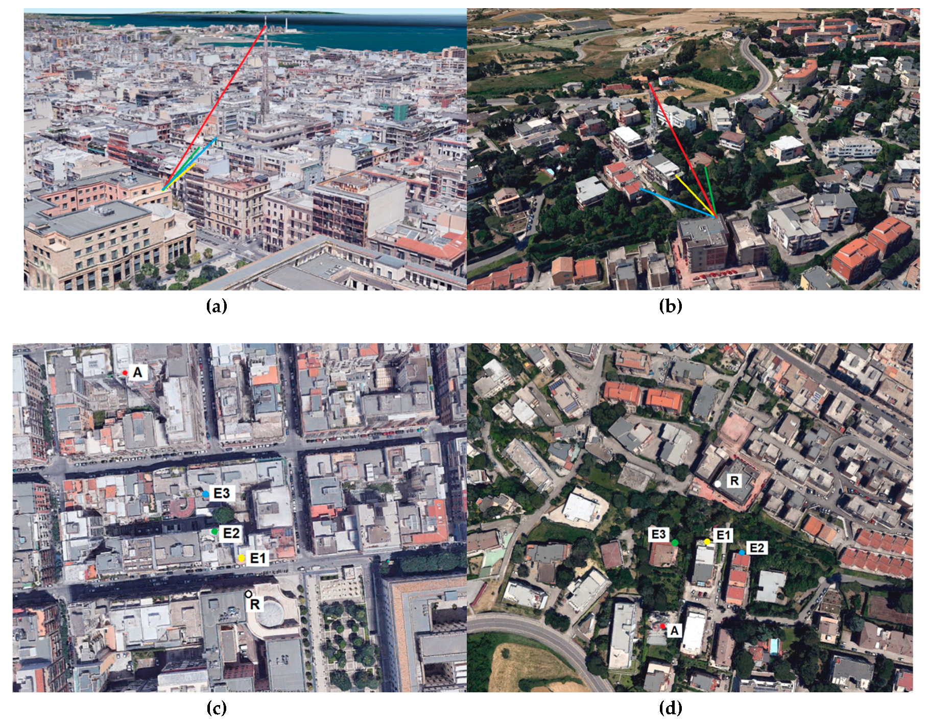
The acquisition geometries are shown in Figure 1; both in case study 1 (Figure 1a) and in case study 2 (Figure 1b), the radar has been installed in front of the telecommunication tower. Antennas with a broad antenna pattern in the vertical plane and a narrow one in the horizontal plane allows the illumination of the whole height of the tower, reducing the contributions from the surrounding buildings to those located within a very small area around the tower.
3.2. Case Studies: Results
The distances in Table 1 are useful for interpreting the NRCS diagrams shown in Figure 3. In particular, the plot in Figure 3a provides the NRCS profile for case study 1. The peaks in the NRCS profile correspond to targets reflecting a larger fraction of the radar microwave signal within a maximum range distance of 200 m. The peaks at range distances smaller than or around 50 m from the radar location correspond to buildings E1 and E2. The peak corresponding to the building E2 is less evident as its surface is almost totally in shadow with respect to the radar; only the top of the building is actually scattering the radar signal. The second group of peaks in the NRCS profiles are between 120 and 150 m from the radar; these correspond to the different elements of the antenna. As far as case study 2 is concerned, the plot in Figure 3b shows the NRCS of all of the targets observed by the radar within a maximum range distance of 500 m. The peaks at range distances smaller than or around 50 m from the radar location correspond to buildings E1, E2 and E3.
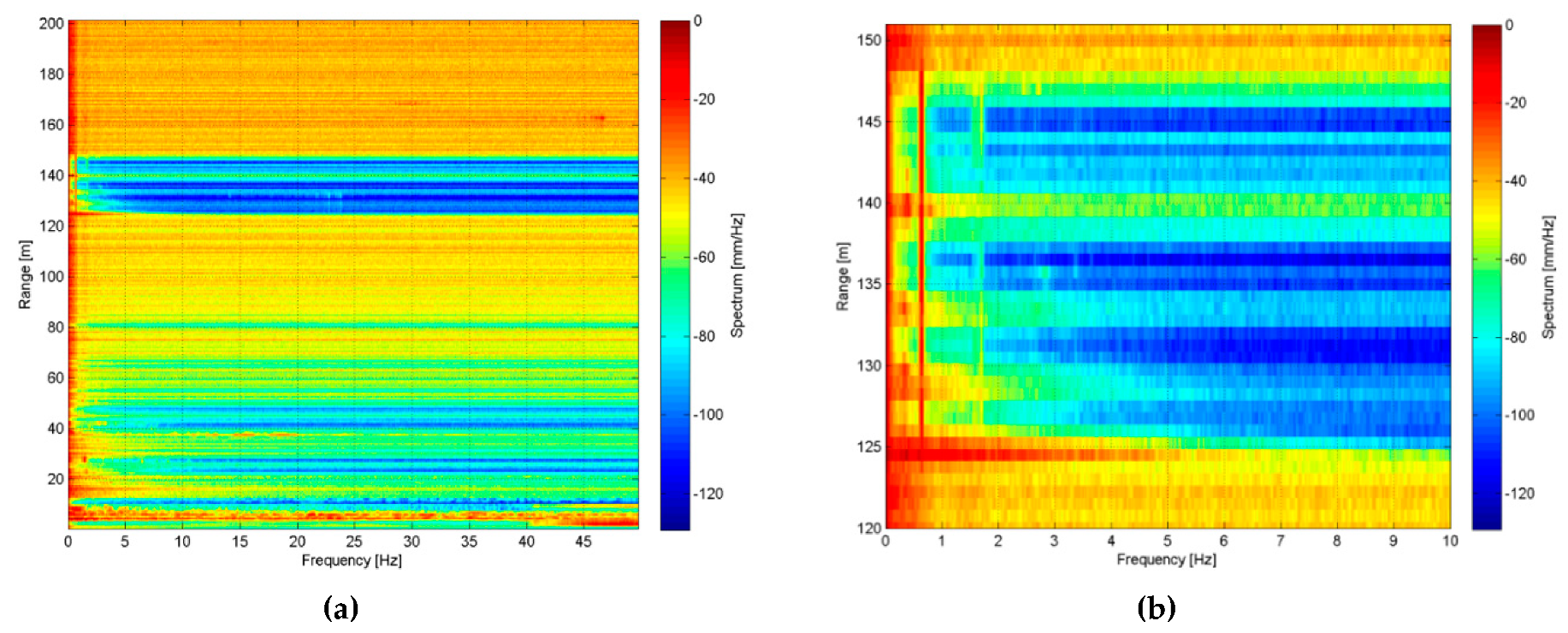
However, the analysis of the NRCS profiles is not enough to clearly identify the targets corresponding to the different portions of the tower. To this end, useful support can be provided by the 2D frequency spectrum of all targets observed by the radar. For instance, Figure 4 displays the 2D spectrum corresponding to case study 1, summarizing the spectra of targets located within the maximum range distance of 200 m from the radar. The observation of this 2D map points out that targets located in the range between 120 and 150 m have a common main peak at the frequency f = 0.64 Hz. The joint analysis of the NRCS (Figure 3a) and frequency spectrum profiles (Figure 4) clearly identifies that the only targets having both a high NRCS and vibrating behaviour are those located at range distances between 120 and 150 m, corresponding to rough estimates of the antenna location obtained from Google© (see Table 1).
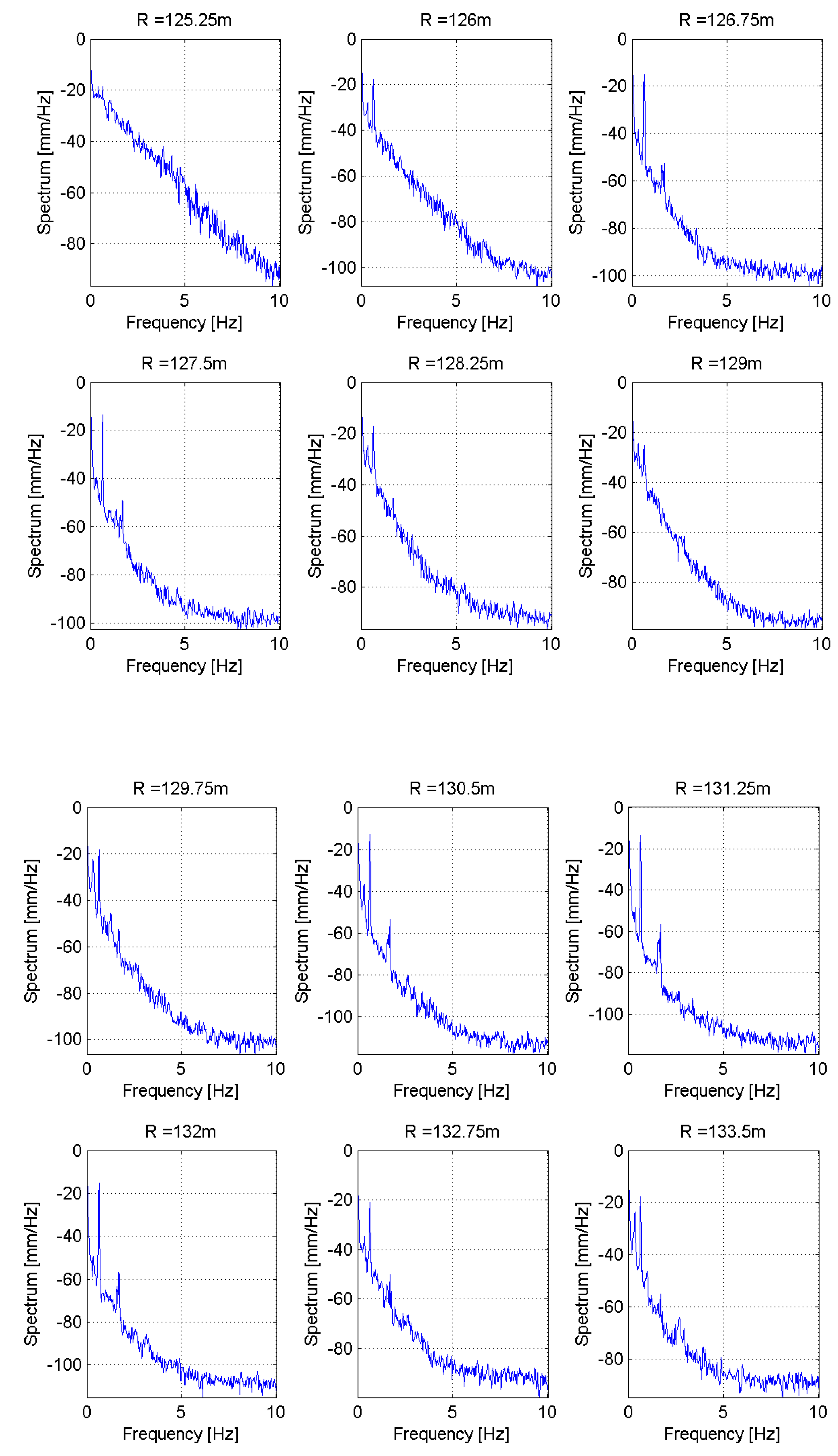
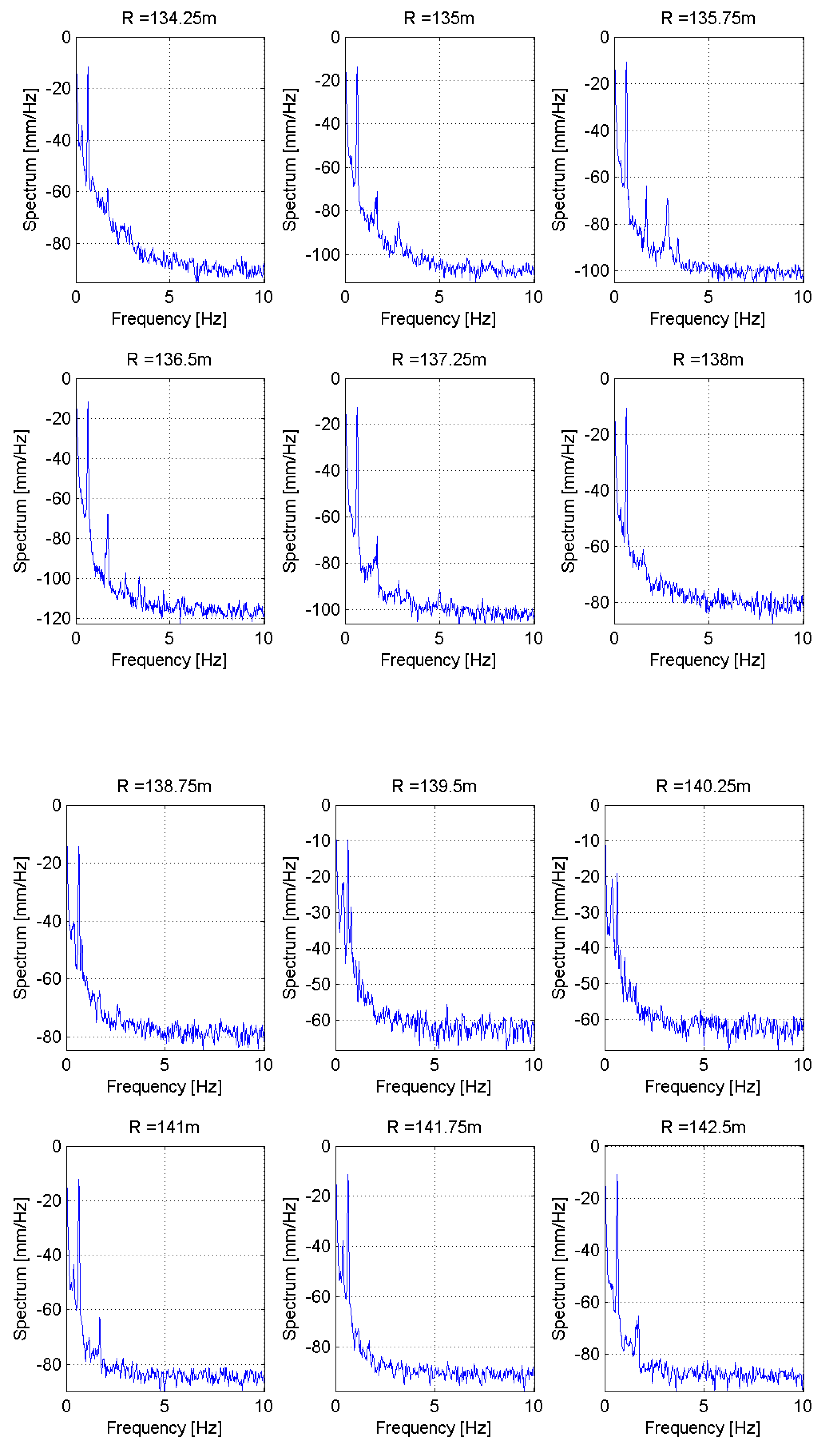
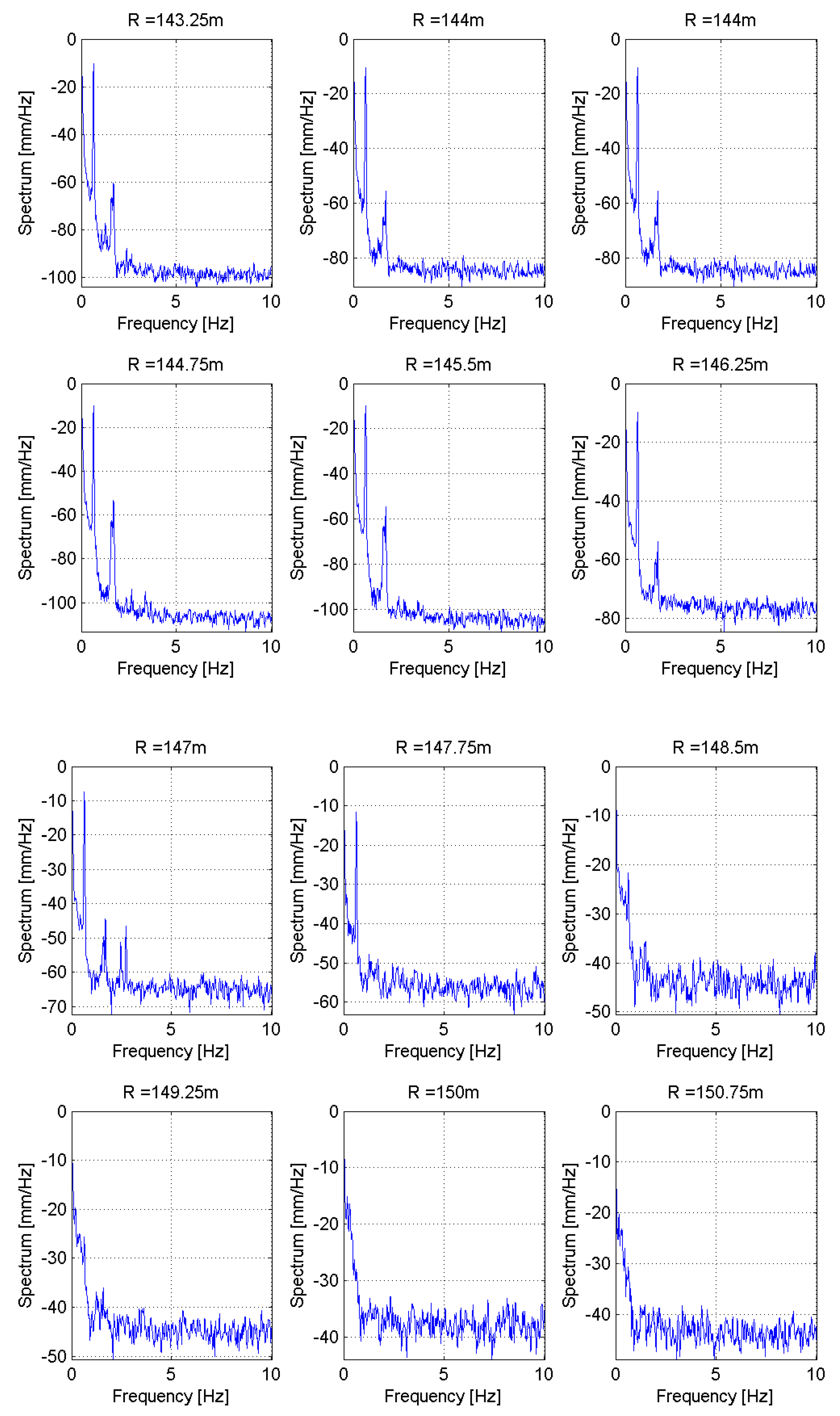
Figure 5 shows, in detail, the 1D spectrum profile of each target within the interval of range distances R corresponding to the antenna. It is found that all of the targets located at distances from 125 to 148 m from the radar are characterized by a vibration frequency of 0.64 Hz. Furthermore, a second peak is observed at the frequency of 1.7 Hz for targets located at distances of 126.75 and 127.50 m; between 130.50 m and 132.00 m; of 136.50 m, 137.25 m and 141.00 m; and between 142.50 and 146.25 m from the radar. Furthermore, targets located at distances of 135.00 m and 135.75 m have peaks at both 1.7 Hz and 2.8 Hz. The target at a distance 147.00 m has three peaks at the frequencies of 1.7, 2.4 and 2.7 Hz. Table 2 summarizes the frequency peaks for all targets corresponding to the antenna and having an oscillating behaviour.
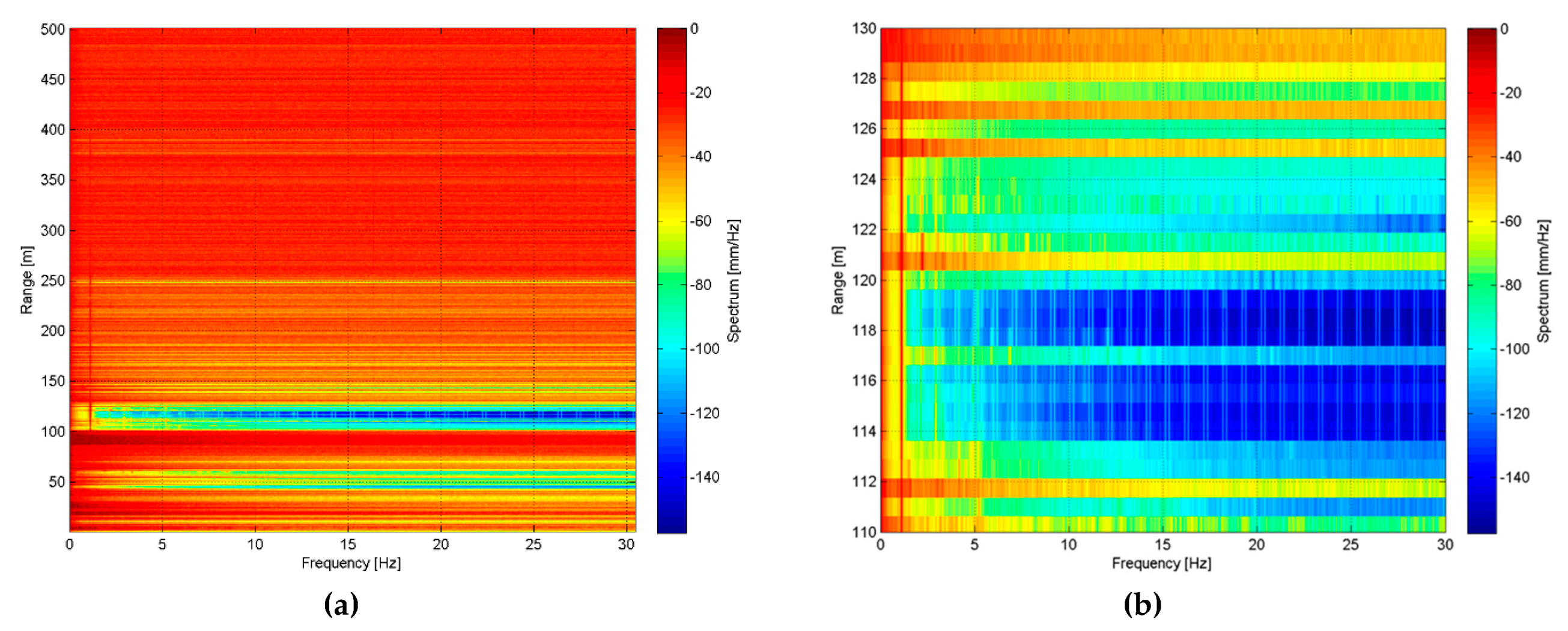
Similar results have been obtained for case study 2. Figure 6 displays the 2D spectrum of targets located within a maximum range of 500 m from the radar. The joint analysis of the NRCS (Figure 3b) and frequency spectrum profiles (Figure 6a) clearly identifies that the only targets having both a high NRCS and an oscillating behaviour are located between 110 and 130 m from the radar.
The details of the 2D spectrum for these targets, supposed to correspond to the antenna, are reported in Figure 6b.
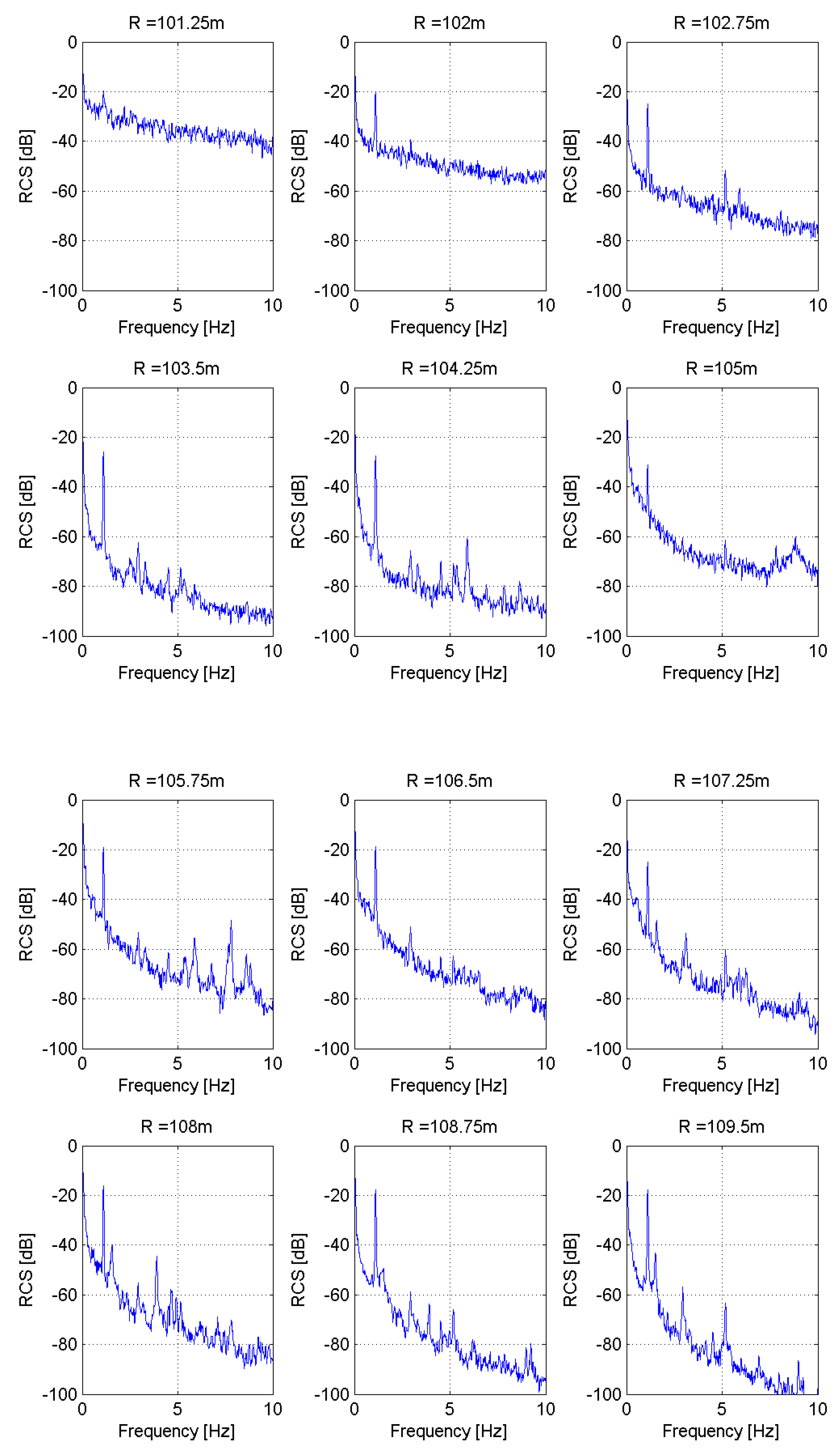
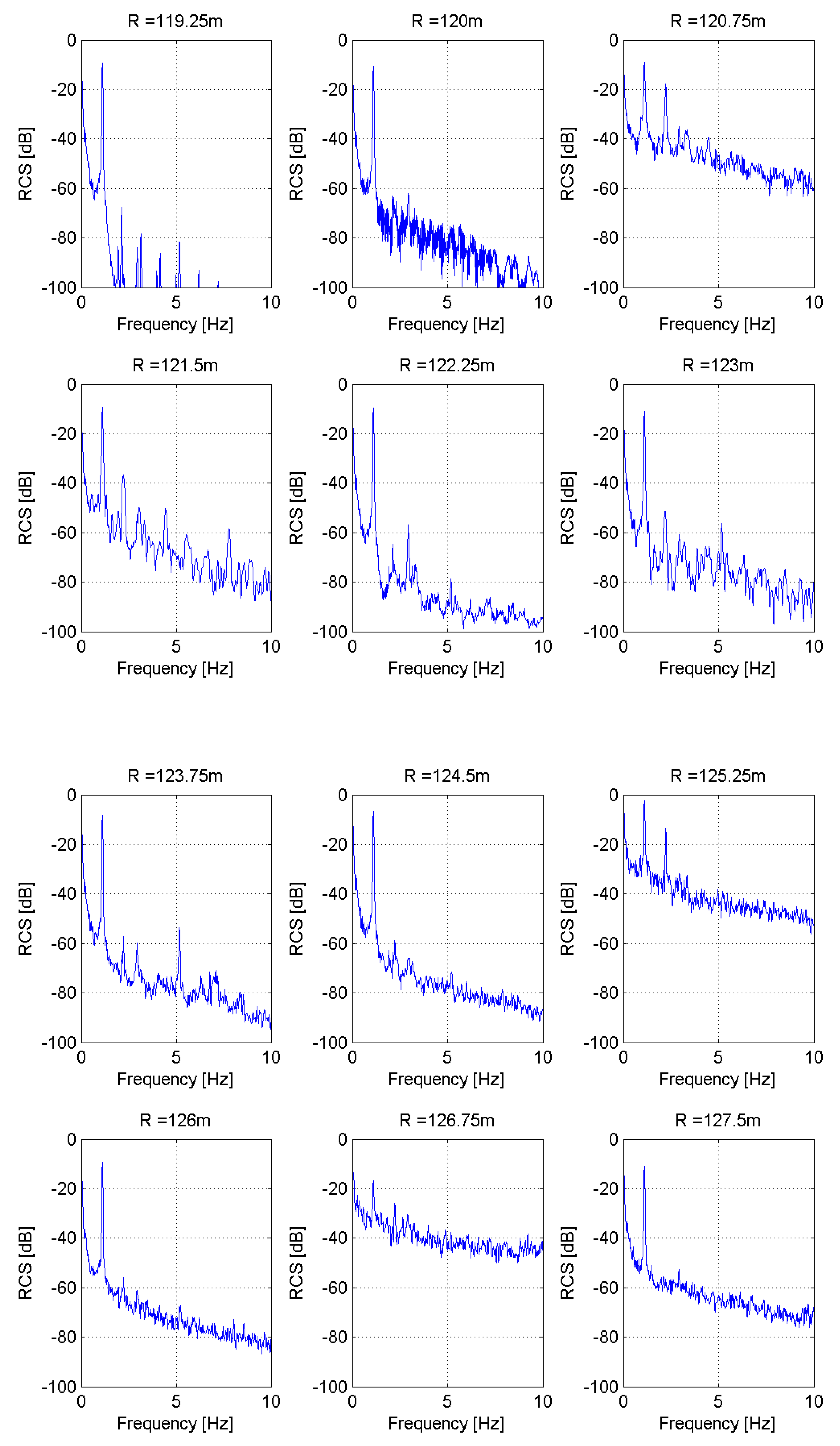
Figure 7 shows, in detail, the 1D spectrum profile of each target within the interval of range distances R corresponding to the antenna. It is found that all of the targets located at distances from 110 to 130 m from the radar are characterized by vibration frequencies of 1.1 Hz. However, in this case, the spectra of the targets present more complex frequency properties. A second peak is observed at the frequency of 2.9 Hz for targets located at distances of 104.25, 106.50, 108.75 and 109.50 m; between 114.00 and 119.00 m, and of 122.25 and 123.75 m from the radar. Furthermore, targets located at distances of 102.75, 104.25, 105.00, 107.25, 108.75, 109.50 and 111.00 m; and between 114.00 and 119.25 m have peaks at 5.2 Hz. Table 3 summarizes the frequency peaks for all of targets corresponding to the antenna and having an oscillating behaviour. The most peculiar characteristic of this case study is the observation of a frequency comb effect with a comb tooth spacing of 1.0 Hz and a carried offset frequency of 6.0 Hz, for targets located at range distances between 114.00 and 119.25 m. All of these frequency peaks are summarized in Table 3.
4. Discussion
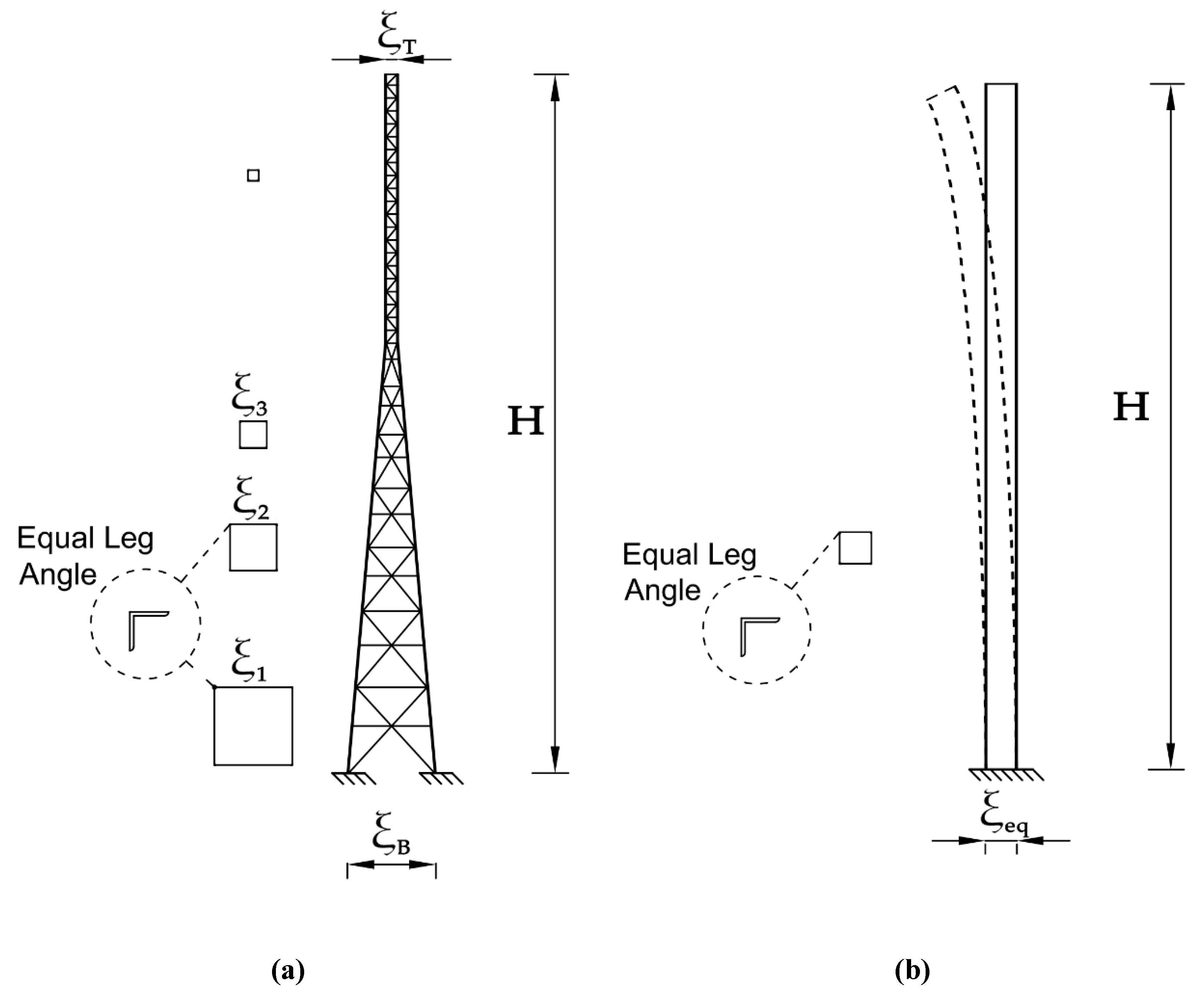
This section discusses the results presented in Section 3. The simplest model for towers and trellises is that of a uniform cantilever vertical beam structure fixed at the base and free to oscillate at the top. The flexional movements are characterized by natural frequencies fn obtained by the following relationship:
where n provides the order of the frequency, E is the Young’s modulus, J is the moment of inertia, m is the unit-length mass and L is the cantilever length, corresponding to the height of the tower [18]. The coefficient αn depends on the kind of constraint at the base of the tower [18]. These values are equal to 1.875, 4.694 and 7.885, depending on n = 1, 2 and 3, respectively [18]. Figure 8 shows a sketch of both the tower and the corresponding uniform cantilever vertical beam, with all relevant parameters. The equivalent cross section ξeq and bending stiffness of the uniform cantilever vertical beam are set in a such a way that the natural frequencies computed in Equation (4) are equal to those provided by the numerical analysis with the Finite Element Method (FEM) code Autodesk Simulation Mechanical software, in the case of flexional vibration. The height of the tower was estimated based on the knowledge of its ground distance from the radar location, provided by Google©, and the interval of range distances derived from the 2D map of the target spectra (Figure 4 and Figure 6). For case study 2, the estimated height of the antenna above the buildings, visible from the radar, is about 51 m, corresponding to an overall height of the antenna of about 65 m. Instead, for case study 1, the height of antenna above the building is 79 m, corresponding a total height of the antenna of 90 m. The structural material, for both towers, is steel S275 (rules UNI EN 10025-2), characterized by a Young’s modulus E of 2.1 ·1011 N/m2.
From the knowledge of the structure stiffness, we can also estimate the expected maximum displacement, assuming a force—e.g., that due to wind—applied to the structures. It is worth noting that Equation (4) can describe only the flexional vibration but not the torsional one. Furthermore, this equation can only be effectively used for continuous systems. However, for a truss beam, as in the towers studied in this paper, Equation (4) provides an approximate solution of the natural frequencies. A more accurate computation of the natural frequencies was obtained by using a 3D model. For evaluating the natural frequencies, the FEM code Autodesk Simulation Mechanical® was used. The telecommunication towers were modelled as a cantilever truss beam, with a fixed joint at the base. They have been described by means of triangular units, the largest of which are divided into triangular subunits. Structural units consist of constant section members that converge into hinged connection nodes. This means that the members are stressed only by traction and compression, while the transmission of bending moments is practically negligible. For the FEM analysis, the data shown in the Table 4 were considered. All members have Equal Leg Angle sections. In the table, the sections are reported by three numbers, which indicate the sizes and thicknesses in millimeters.
Five natural frequencies, corresponding to different vibration modes, have been obtained. Due to the geometry of the tower, we take into account the first and the fifth ones. The first mode given by the FEM code corresponds to oscillations in a vertical plane of symmetry of the tower. The second mode is related to oscillations in the vertical plane of symmetry, perpendicular to the first mode plane. The third and fourth modes are combinations of flexural and torsional oscillations. The fifth one is related to torsional effects.
In the first case study, corresponding to the tower with H = 90 m, the FEM code estimated a frequency for the first mode equal to f1 = 0.6 Hz, which is the vibration frequency measured by the GBSAR. As far as the second case study is concerned, the frequency of first mode obtained by the FEM code is f1 = 1.0 Hz, close to the vibration frequency measured by the GB RAR, which was 1.1 Hz (see Table 3). In both cases, the vibration frequencies of the first mode, provided by the FEM code, correspond to frequency measured by the GB-RAR in all range bins covering the antenna, and it can be concluded that they correspond to a vibration mode of the whole tower.
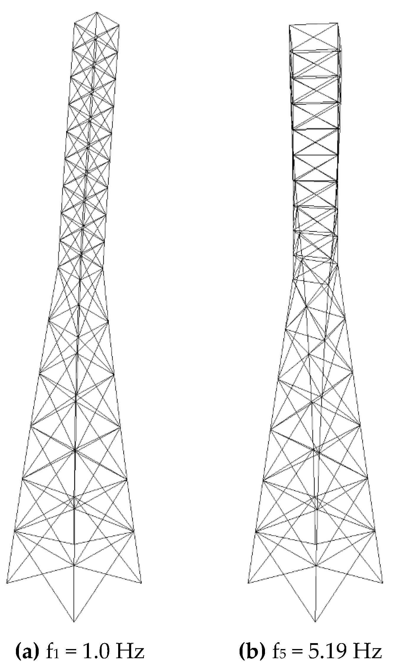
In the following part, we focus on the second case, corresponding to the shortest tower and characterized by a larger number of antennas installed on it. In fact, the weight of these antennas and their impact on the vibration modes of the towers have not been modelled in the FEM code. It was found that besides the first and second modes having equal frequencies, the fifth mode also has a frequency close to that of those measured by the GB-RAR. In particular, for the second case study, the FEM code computed a vibration frequency f5 = 5.2 Hz. This vibration mode is more evident in the upper part of the cantilever structure, as can be observed in Figure 9, where both the first and fifth vibration modes are shown. In terms of the comparison with the vibration frequencies measured by the GB-RAR, as summarized in Table 3, it was found that a vibration frequency in the range of 5.1 to 5.2 Hz was measured in fifteen of the forty-two range bins covering the visible part of the tower. In particular, a vibration frequency of 5.2 Hz was measured by GB-RAR, corresponding to the part of the tower located at a range distance of 124.00 m, and corresponding to a height of 65 m.
However, the analysis of Table 3 shows many other vibration frequencies that characterize the different portions of the tower. These frequencies were not found in the simple FEM analysis. The differences between the FEM analysis results and GBSAR measurements could be explained in terms of:
- (1)
- The schematization of constraints differing slightly from the actual connections of the tower elements;
- (2)
- The intensities and positions of the point loads due to the parabolic, planar and linear antennas and consequently, their influence on the wind loads, being known only approximately.
On the other hand, the presence of several antennas fixed at different heights to that of the tower amplifies the torsional displacements. This could explain why the vibration frequency of the fifth mode can be observed only for some sections of the tower.
Besides this, it is worth noting that the terminal spar has a different cross section with respect to the lower part of the antenna. Its distance from the GB-RAR position is 120.00 to 130.00 m, and the target, at a distance 130.00 m, is the very top of the structure. Thus, along with the first and second order of frequency, it should be expected more complex vibration modes, due to the type of connection between the tower and the spar, which lies partially into the tower. A more accurate assessment could be done by using a very detailed model and a FEM solver.
To conclude, we point out the frequency comb effect with a comb tooth spacing of 1.0 Hz and a carried offset frequency of 1.0 Hz, which has been observed in the second case study, for targets located at range distances between 114.00 and 119.25 m. This effect could be related to a modulation in the amplitude and/or phase in correspondence of the targets on the antenna located between 114.00 and 119.25 m from the radar. One possible explanation for this are the transmitting antennas deployed on the tower of the second case study. As a simple qualitative model, if we suppose that the antennas are transmitting the signal in the same frequency band of the radar, modulated in phase as
where A is the amplitude modulation, t is the time and f1 = 1 Hz, we find that its spectrum shows a typical comb effect, as reported in Figure 10. We observe that the number of frequency peaks depends on the modulation amplitude.
However, an explanation of the physical mechanisms behind the observed frequency comb effect will not be further discussed, as it is beyond the aim of this work and needs a more advanced modelling study.
5. Conclusions
In this work, we proposed a methodology for the quick inspection of trellises and telecommunication towers based on the ground-based radar interferometry. Two case studies are presented. In the first, we show how the joint analysis of the NRCS profiles and 2D maps of target spectra can easily identify the interval of range distances covering the portion of the tower visible from the radar location. This means that a rough estimate of the tower geometry can be obtained directly in the field without any precise topographic survey. This is useful for both clearly distinguishing the signal related to the tower and for a quick interpretation of the vibration frequencies and displacements measured by the radar, in terms of the height of the tower. The frequency peaks and the displacement profiles of all targets, corresponding to the different portions of the towers, are estimated. A qualitative comparison with a simple FEM analysis, using the tower heights provided by the joint analysis of the NRCS and vibration spectra, was carried out. It was found that the GB-RAR measurements identified the first five frequency modes of towers modelled as a cantilever truss beam. The proposed methodology can also be applied to the quick inspection of power line pylons.
Author Contributions
Conceptualization, G.N.; methodology, G.N.; software, O.M. and G.N.; investigation, S.A., O.M., G.N. and G.P.; writing—original draft preparation, S.A., G.N. and G.P.; writing—review and editing, S.A., G.N. and G.P.; funding acquisition: O.M. All authors have read and agreed to the published version of the manuscript.
Funding
This research received no external funding.
Acknowledgments
Authors acknowledge Telecom Italia S.p.A. and HSH Informatica & Cultura S.r.l. for support during data acquisition.
Conflicts of Interest
The authors declare no conflict of interest. The funders had no role in the design of the study; in the collection, analyses, or interpretation of data; in the writing of the manuscript, or in the decision to publish the results.
References
- Amiri, M.M.; Yahyai, M. Estimation of damping ratio of TV towers based on ambient vibration monitoring. Struct. Des. Tall Spéc. Build. 2011, 22, 862–875. [Google Scholar] [CrossRef]
- Matikainen, L.; Lehtomäki, M.; Ahokas, E.; Hyyppä, J.; Karjalainen, M.; Jaakkola, A.; Kukko, A.; Heinonen, T. Remote sensing methods for power line corridor surveys. ISPRS J. Photogramm. Remote. Sens. 2016, 119, 10–31. [Google Scholar] [CrossRef] [Green Version]
- Pieraccini, M. Monitoring of Civil Infrastructures by Interferometric Radar: A Review. Sci. World J. 2013, 2013, 1–8. [Google Scholar] [CrossRef] [PubMed]
- Di Pasquale, A.; Corsetti, M.; Guccione, P.; Lugli, A.; Nicoletti, M.; Nico, G.; Zonno, M. Ground-based SAR interferometry as a supporting tool in natural and man-made disasters. In Proceedings of the 33rd EARSel Symposium, Matera, Italy, 3–6 June 2013; pp. 173–186. [Google Scholar]
- Nico, G.; Borrelli, L.; Di Pasquale, A.; Antronico, L.; Gullà, G. Monitoring of an Ancient Landslide Phenomenon by GBSAR Technique in the Maierato Town (Calabria, Italy). Eng. Geol. Soc. Territ. 2015, 2, 129–133. [Google Scholar]
- Anghel, A.; Ding, Z.; Nies, H.; Loffeld, O.; Atencia, D.; Huaman, S.G.; Medella, A.; Moreira, J.; Tudose, M.; Cacoveanu, R.; et al. Compact Ground-Based Interferometric Synthetic Aperture Radar: Short-Range Structural Monitoring. IEEE Signal Process. Mag. 2019, 36, 42–52. [Google Scholar] [CrossRef]
- Mascolo, L.; Nico, G.; Di Pasquale, A.; Pitullo, A. Use of advanced SAR monitoring techniques for the assessment of the behaviour of old embankment dams. SPIE Remote Sens. 2014, 9245, 92450. [Google Scholar]
- Scaioni, M.; Marsella, M.; Crosetto, M.; Tornatore, V.; Wang, J. Geodetic and Remote-Sensing Sensors for Dam Deformation Monitoring. Sensors 2018, 18, 3682. [Google Scholar] [CrossRef] [PubMed] [Green Version]
- Nico, G.; Cifarelli, G.; Miccoli, G.; Soccodato, F.M.; Feng, W.; Sato, M.; Miliziano, S.; Marini, M. Measurement of Pier Deformation Patterns by Ground-Based SAR Interferometry: Application to a Bollard Pull Trial. IEEE J. Ocean. Eng. 2018, 43, 822–829. [Google Scholar] [CrossRef]
- Pieraccini, M.; Fratini, M.; Parrini, F.; Macaluso, G.; Atzeni, C. High-speed CW step-frequency coherent radar for dynamic monitoring of civil engineering structures. Electron. Lett. 2004, 40, 907. [Google Scholar] [CrossRef]
- Artese, S.; Achilli, V.; Zinno, R. Monitoring of Bridges by a Laser Pointer: Dynamic Measurement of Support Rotations and Elastic Line Displacements: Methodology and First Test. Sensors 2018, 18, 338. [Google Scholar] [CrossRef] [PubMed] [Green Version]
- Artese, S. THE Survey of the san francesco bridge by santiago calatrava in cosenza, Italy. ISPRS Int. Arch. Photogramm. Remote. Sens. Spat. Inf. Sci. 2019, 33–37. [Google Scholar] [CrossRef] [Green Version]
- Pieraccini, M.; Fratini, M.; Parrini, F.; Atzeni, C.; Bartoli, G. Interferometric radar vs. accelerometer for dynamic monitoring of large structures: An experimental comparison. NDT E Int. 2008, 41, 258–264. [Google Scholar] [CrossRef]
- Artese, S.; Nico, G. TLS and GB-RAR Measurements of Vibration Frequencies and Oscillation Amplitudes of Tall Structures: An Application to Wind Towers. Appl. Sci. 2020, 10, 2237. [Google Scholar] [CrossRef] [Green Version]
- Di Pasquale, A.; Nico, G.; Pitullo, A.; Prezioso, G. Monitoring Strategies of Earth Dams by Ground-Based Radar Interferometry: How to Extract Useful Information for Seismic Risk Assessment. Sensors 2018, 18, 244. [Google Scholar] [CrossRef] [PubMed] [Green Version]
- Farrar, C.R.; Doebling, S.W.; Nix, D.A. Vibration–based structural damage identification. Philos. Trans. R. Soc. A Math. Phys. Eng. Sci. 2001, 359, 131–149. [Google Scholar] [CrossRef]
- Farrar, C.R.; Worden, K. An introduction to structural health monitoring. Philos. Trans. R. Soc. A Math. Phys. Eng. Sci. 2006, 365, 303–315. [Google Scholar] [CrossRef] [PubMed]
- Thomson, W.T. Theory of Vibration with Application; Kindersley Publishing, Inc.: London, UK, 2007. [Google Scholar]
Figure 1.
A view of the telecommunication tower from the radar installation site: (a) case study 1, (b) case study 2.
Figure 1.
A view of the telecommunication tower from the radar installation site: (a) case study 1, (b) case study 2.

Figure 2.
Google© images of the study areas 1 (a) and 2 (b). The radar positions and towers are denoted by R and A, respectively. The nearby buildings between the radar and the telecommunication tower are denoted by E1, E2 and E3. (c) and (d) are the same as (a) and (b), but seen in planimetry (see also Table 1).

Figure 3.
A Normalized Radar Cross-Section (NRCS) of targets observed by the radar in case studies 1 (a) and 2 (b). The maximum range distances were set to 200 and 500 m, respectively.
Figure 3.
A Normalized Radar Cross-Section (NRCS) of targets observed by the radar in case studies 1 (a) and 2 (b). The maximum range distances were set to 200 and 500 m, respectively.

Figure 4.
Case study 1: (a) the frequency spectra of targets observed by the radar within a range distance of 200 m; (b) detail of the frequency spectra, referring to targets located in the range interval (120 m, 150 m).
Figure 4.
Case study 1: (a) the frequency spectra of targets observed by the radar within a range distance of 200 m; (b) detail of the frequency spectra, referring to targets located in the range interval (120 m, 150 m).

Figure 5.
Case study 1: the frequency spectrum profiles of targets located between 120 and 150 m from the radar.
Figure 5.
Case study 1: the frequency spectrum profiles of targets located between 120 and 150 m from the radar.


Figure 6.
Case study 2: (a) the frequency spectra of targets observed by the radar within the range distance of 500 m; (b) details of the frequency spectra, referring to targets located in the range interval (110 m, 130 m).
Figure 6.
Case study 2: (a) the frequency spectra of targets observed by the radar within the range distance of 500 m; (b) details of the frequency spectra, referring to targets located in the range interval (110 m, 130 m).

Figure 7.
Case study 2: the frequency spectrum profiles of targets located between 110 and 130 m from the radar.
Figure 7.
Case study 2: the frequency spectrum profiles of targets located between 110 and 130 m from the radar.


Figure 8.
A sketch of (a) the tower structure used in the numerical analysis with the FEM code Autodesk Simulation Mechanical software and (b) the uniform cantilever vertical beam used in Equation (4). The cross sections at the bottom, top and at three intermediate heights of the tower are denoted by ξT, ξB, ξ1, ξ2 and ξ3, respectively. The height of both the tower and the cantilever beam is denoted by H. The equivalent cross section ξeq and bending stiffness of the uniform cantilever vertical beam are set in a such a way that the natural frequencies computed in Equation (4) are equal to those provided by the numerical analysis with the FEM code, in the case of flexional vibration.

Figure 9.
Case study 2: the deformations of the tower due to the first (a) and fifth (b) vibration modes. Deformations are exaggerated; the scale is arbitrary.
Figure 9.
Case study 2: the deformations of the tower due to the first (a) and fifth (b) vibration modes. Deformations are exaggerated; the scale is arbitrary.

Figure 10.
The spectrum of the signal modulated in phase, as in Equation (5), for three different values of the modulation amplitude A.
Figure 10.
The spectrum of the signal modulated in phase, as in Equation (5), for three different values of the modulation amplitude A.


Table 1.
The distances between the radar location R and the targets A (tower), E1, E2 and E3 (buildings), for the two case studies.
Table 1.
The distances between the radar location R and the targets A (tower), E1, E2 and E3 (buildings), for the two case studies.
| Target | (Case Study 1) | (Case Study 2) |
|---|---|---|
| Distance [m] | Distance [m] | |
| A | 125 | 115 |
| E1 | 24 | 46 |
| E2 | 42 | 53 |
| E3 | 60 | 52 |
Table 2.
Case study 1: the frequency peaks of targets corresponding to the antenna.
| Range Distance [m] | Frequency [Hz] | Range Distance [m] | Frequency [Hz] |
|---|---|---|---|
| 126.00 | 0.6 | 138.00 | 0.6 |
| 126.75 | 0.6; 1.7 | 138.75 | 0.6 |
| 127.50 | 0.6; 1.7 | 139.50 | 0.6 |
| 128.25 | 0.6 | 140.25 | 0.6 |
| 129.00 | 0.6 | 141.00 | 0.6; 1.7 |
| 129.75 | 0.6 | 141.75 | 0.6 |
| 130.50 | 0.6; 1.7 | 142.50 | 0.6; 1.7 |
| 131.25 | 0.6; 1.7 | 143.25 | 0.6; 1.7 |
| 132.00 | 0.6; 1.7 | 144.00 | 0.6; 1.7 |
| 132.75 | 0.6 | 144.75 | 0.6; 1.7 |
| 133.50 | 0.6 | 145.50 | 0.6; 1.7 |
| 134.25 | 0.6 | 146.25 | 0.6; 1.7 |
| 135.00 | 0.6; 2.8 | 147.00 | 0.6; 1.7; 2.4; 2.7 |
| 135.75 | 0.6; 1.7; 2.8 | 147.75 | 0.6 |
| 136.50 | 0.6; 1.7 | 148.50 | 0.6 |
| 137.25 | 0.6; 1.7 |
Table 3.
Case study 2: the frequency peaks of targets corresponding to the antenna.
| Range Distance [m] | Frequency [Hz] |
|---|---|
| 102.00 | 1.1 |
| 102.75 | 1.1; 5.2; 5.9 |
| 103.50 | 1.1 |
| 104.25 | 1.1; 2.9; 3.3; 4.5; 5.2; 5.3; 5.9 |
| 105.00 | 1.1; 5.2; 8.8 |
| 105.75 | 1.1; 4.5; 5.3; 5.4; 6.0; 6.8; 7.7; 7.8; 8.6; 8.8 |
| 106.50 | 1.1; 2.9 |
| 107.25 | 1.1; 1.6; 3.1; 5.2 |
| 108.00 | 1.1; 1.6; 3.9 |
| 108.75 | 1.1; 2.9; 3.9; 5.2; 9.0; 9.2 |
| 109.50 | 1.1; 1.5; 2.9; 5.2 |
| 110.25 | 1.1 |
| 111.00 | 1.1; 5.2 |
| 111.75 | 1.1 |
| 112.50 | 1.1; 1.5; 4.2 |
| 113.25 | 1.1; 4.2; 4.9 |
| 114.00 | 1.1; 2.1; 2.9; 3.1; 3.3; 4.0; 4.1; 5.2 Comb effect with Δf = 1.0 Hz and f0 = 1.0 Hz |
| 114.75 | 1.1; 2.1; 2.9; 3.1; 3.3; 4.0; 4.1; 5.2 Comb effect with Δf = 1.0 Hz and f0 = 1.0 Hz |
| 115.50 | 1.1; 2.1; 2.9; 3.1; 3.3; 4.0; 4.1; 5.2 Comb effect with Δf = 1.0 Hz and f0 = 1.0 Hz |
| 116.25 | 1.1; 2.1; 2.9; 3.1; 3.3; 3.9; 4.2; 5.2 Comb effect with Δf = 1.0 Hz and f0 = 1.0 Hz |
| 117.00 | 1.1; 2.2; 2.9; 5.9; 6.9; 12.0; 12.7; 13.7; 20.0 |
| 117.75 | 1.1; 2.1; 2.9; 3.1; 3.3; 4.0; 4.2; 5.2 Comb effect with Δf = 1.0 Hz and f0 = 1.0 Hz |
| 118.50 | 1.1; 2.1; 2.9; 3.1; 3.3; 4.0; 4.2; 5.2 Comb effect with Δf = 1.0 Hz and f0 = 1.0 Hz |
| 119.25 | 1.1; 2.1; 2.9; 3.1; 3.3; 4.0; 4.2; 5.2 Comb effect with Δf = 1.0 Hz and f0 = 1.0 Hz |
| 120.00 | 1.1 |
| 120.75 | 1.1; 2.2 |
| 121.50 | 1.1; 2.2; 7.8 |
| 122.25 | 1.1; 2.1; 2.9 |
| 123.00 | 1.1 |
| 123.75 | 1.1; 2.2; 2.9; 5.2 |
| 124.50 | 1.1 |
| 125.25 | 1.1; 2.2 |
| 126.00 | 1.1 |
| 126.75 | 1.1 |
| 127.50 | 1.1 |
| 128.25 | 1.1 |
| 129.00 | 1.1 |
| 129.75 | 1.1 |
Table 4.
The modelling design of telecommunication towers used for FEM analysis.
| Case Study 1 | Case Study 2 | |
|---|---|---|
| E [N/m2] | 2.1 × 10¹¹ | 2.1 × 10¹¹ |
| Legs members sections [mm] | 140 × 140 × 14 120 × 120 × 12 80 × 80 × 80 | 120 × 120 × 12 80 × 80 × 8 |
| Diagonal members [mm] | 80 × 80 × 7 60 × 60 × 6 55 × 55 × 5 50 × 50 × 4 45 × 45 × 4 | 80 × 80 × 7 60 × 60 × 6 55 × 55 × 5 50 × 50 × 4 45 × 45 × 4 |
| Horizontal members [mm] | 60 × 60 × 6 50 × 50 × 5 45 × 45 × 4 | 45 × 45 ×5 |
| L [m] | 90 | 65 |
© 2020 by the authors. Licensee MDPI, Basel, Switzerland. This article is an open access article distributed under the terms and conditions of the Creative Commons Attribution (CC BY) license (http://creativecommons.org/licenses/by/4.0/).
Share and Cite
MDPI and ACS Style
Nico, G.; Prezioso, G.; Masci, O.; Artese, S. Dynamic Modal Identification of Telecommunication Towers Using Ground Based Radar Interferometry. Remote Sens. 2020, 12, 1211. https://0-doi-org.brum.beds.ac.uk/10.3390/rs12071211
AMA Style
Nico G, Prezioso G, Masci O, Artese S. Dynamic Modal Identification of Telecommunication Towers Using Ground Based Radar Interferometry. Remote Sensing. 2020; 12(7):1211. https://0-doi-org.brum.beds.ac.uk/10.3390/rs12071211
Chicago/Turabian StyleNico, Giovanni, Giuseppina Prezioso, Olimpia Masci, and Serena Artese. 2020. "Dynamic Modal Identification of Telecommunication Towers Using Ground Based Radar Interferometry" Remote Sensing 12, no. 7: 1211. https://0-doi-org.brum.beds.ac.uk/10.3390/rs12071211
Note that from the first issue of 2016, this journal uses article numbers instead of page numbers. See further details here.