Semantic Labeling in Remote Sensing Corpora Using Feature Fusion-Based Enhanced Global Convolutional Network with High-Resolution Representations and Depthwise Atrous Convolution

Abstract

One of the fundamental tasks in remote sensing is the semantic segmentation on the aerial and satellite images. It plays a vital role in applications, such as agriculture planning, map updates, route optimization, and navigation. The state-of-the-art model is the Enhanced Global Convolutional Network (GCN152-TL-A) from our previous work. It composes two main components: (i) the backbone network to extract features and ($ii$) the segmentation network to annotate labels. However, the accuracy can be further improved, since the deep learning network is not designed for recovering low-level features (e.g., river, low vegetation). In this paper, we aim to improve the semantic segmentation network in three aspects, designed explicitly for the remotely sensed domain. First, we propose to employ a modern backbone network called “High-Resolution Representation (HR)” to extract features with higher quality. It repeatedly fuses the representations generated by the high-to-low subnetworks with the restoration of the low-resolution representations to the same depth and level. Second, “Feature Fusion (FF)” is added to our network to capture low-level features (e.g., lines, dots, or gradient orientation). It fuses between the features from the backbone and the segmentation models, which helps to prevent the loss of these low-level features. Finally, “Depthwise Atrous Convolution (DA)” is introduced to refine the extracted features by using four multi-resolution layers in collaboration with a dilated convolution strategy. The experiment was conducted on three data sets: two private corpora from Landsat-8 satellite and one public benchmark from the “ISPRS Vaihingen” challenge. There are two baseline models: the Deep Encoder-Decoder Network (DCED) and our previous model. The results show that the proposed model significantly outperforms all baselines. It is the winner in all data sets and exceeds more than 90% of $F1$: 0.9114, 0.9362, and 0.9111 in two Landsat-8 and ISPRS Vaihingen data sets, respectively. Furthermore, it achieves an accuracy beyond 90% on almost all classes.

1. Introduction

Semantic segmentation in a medium resolution (MR) image, e.g., a Landsat-8 (LS-8) image, and very high resolution (VHR) images, e.g., aerial images, is a long-standing issue and problem in the domains of remote sensing-based information. Natural objects such as roads, water, forests, urban, and agriculture fields regions are operated in various tasks such as route optimization to create imperative remotely sensed applications.

Deep learning, especially the Deep Convolutional Neural Network (CNN), is an acclaimed approach for automatic feature learning. In previous research, CNN-based segmentation approaches are proposed to perform semantic labeling [1,2,3,4,5]. To achieve such a challenging task, features from various levels are fused together [5,6,7]. Specifically, a lot of approaches fuse low-level and high-level features together [5,6,7,8,9]. In remote sensing corpora, ambiguous human-made objects need high-level features for a more well-defined recognition (e.g., roads, building roofs, and bicycle runways), while fine-structured objects (e.g., low vegetations, cars, and trees) could benefit from comprehensive low-level features [10]. Consequently, the performance will be affected by the different numbers of layers and/or different fusion techniques of the deep learning model.

In recent years, the Global Convolutional Network (GCN) [11], the modern CNN, has been introduced, in which the valid receptive field and large filter enable dense connections between pixel-based classifiers and activation maps, which enhances the capability to cope with different transformations. The GCN is aimed at addressing both the localization and segmentation problems for image labeling and presents Boundary Refinement (BR) to refine the object boundaries further as well. 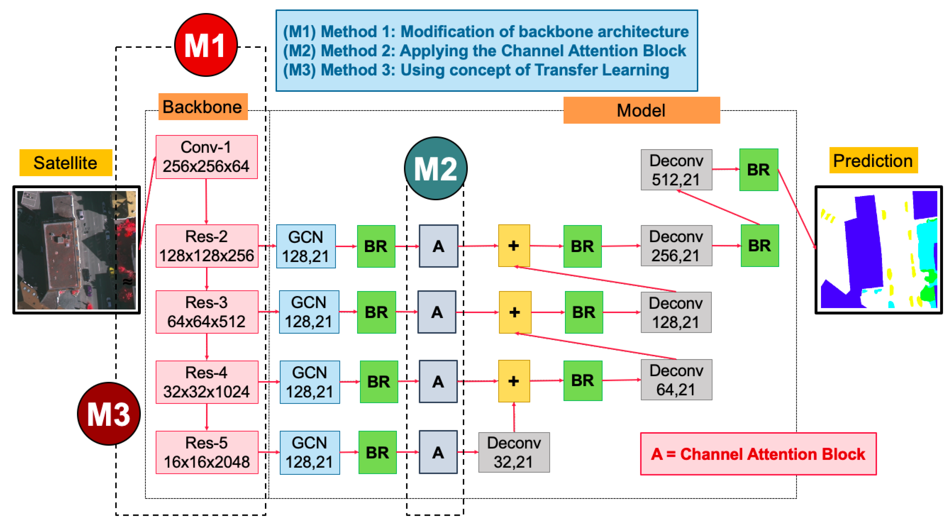Our previous work [12] extended the GCN by enhancing three approaches as illustrated in Figure 1 and Figure 2. First, “Transfer Learning” [13,14,15] was employed to relieve the shortage problem. Next, we varied the backbone network using ResNet152, ResNet101, and ResNet50. Last, “Channel Attention Block” [16,17] was applied to allocate CNN parameters for the output of each layer in the front-end of the deep learning architecture.

Nevertheless, our previous work still disregards the local context, such as low-level features in each stage. Moreover, most feature fusion methods are just a summation of the features from adjacent stages and they do not consider the representations of diversity (critical for the performance of the CNN). This leads to unpredictable results that suffer from measuring the performance such as the $F1$ score. This, in fact, is the inspiration for this work.

In summary, although the current enhanced Global Convolutional Network (GCN152-TL-A) method [12] has achieved significant breakthroughs in semantic segmentation on remote sensing corpora, it is still laborious to manually label the MR images in river and pineapple areas and the VHR images in low vegetation and car areas. The two reasons are as follows: $\left(i\right)$ previous approaches are less efficient to recover low-level features for accurate labeling, and $\left(ii\right)$ they ignore the low-level features learned by the backbone network’s shallow layers with long-span connections, which is caused by semantic gaps in different-level contexts and features.

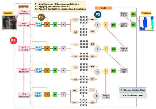
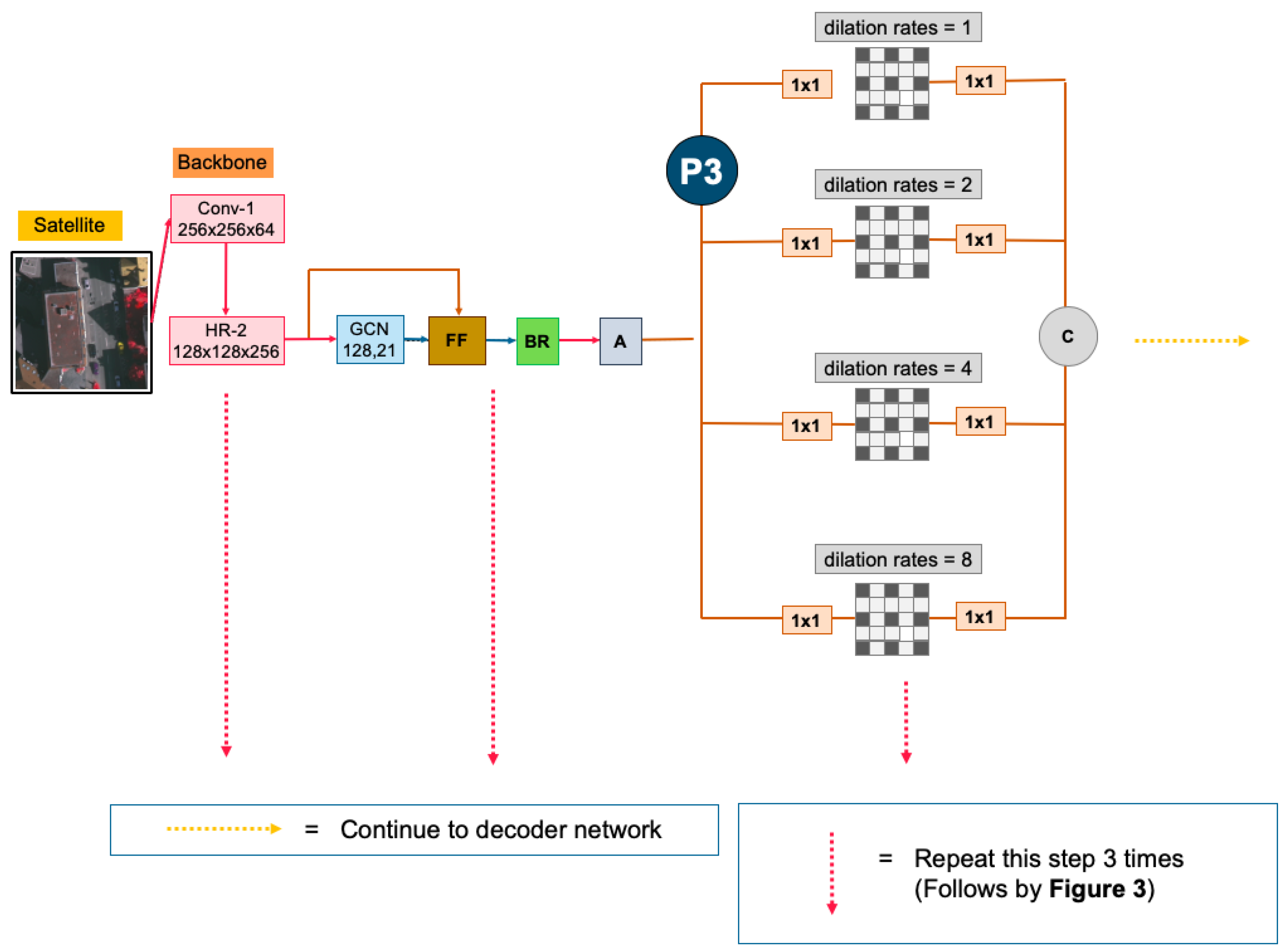
In this paper, motivated by the above observation, we propose a novel Global Convolutional Network (“HR-GCN-FF-DA”) for segmenting multi-objects from satellite and aerial images, as illustrated in Figure 3. This paper aims to further improve the state-of-the-art on semantic segmentation in MR and VHR images. In this paper, there are three contributions, as follows:

• Applying a new backbone called “High-Resolution Representation (HR)” to GCN for the restoration of the low-resolution representations of the same depth and similar level.
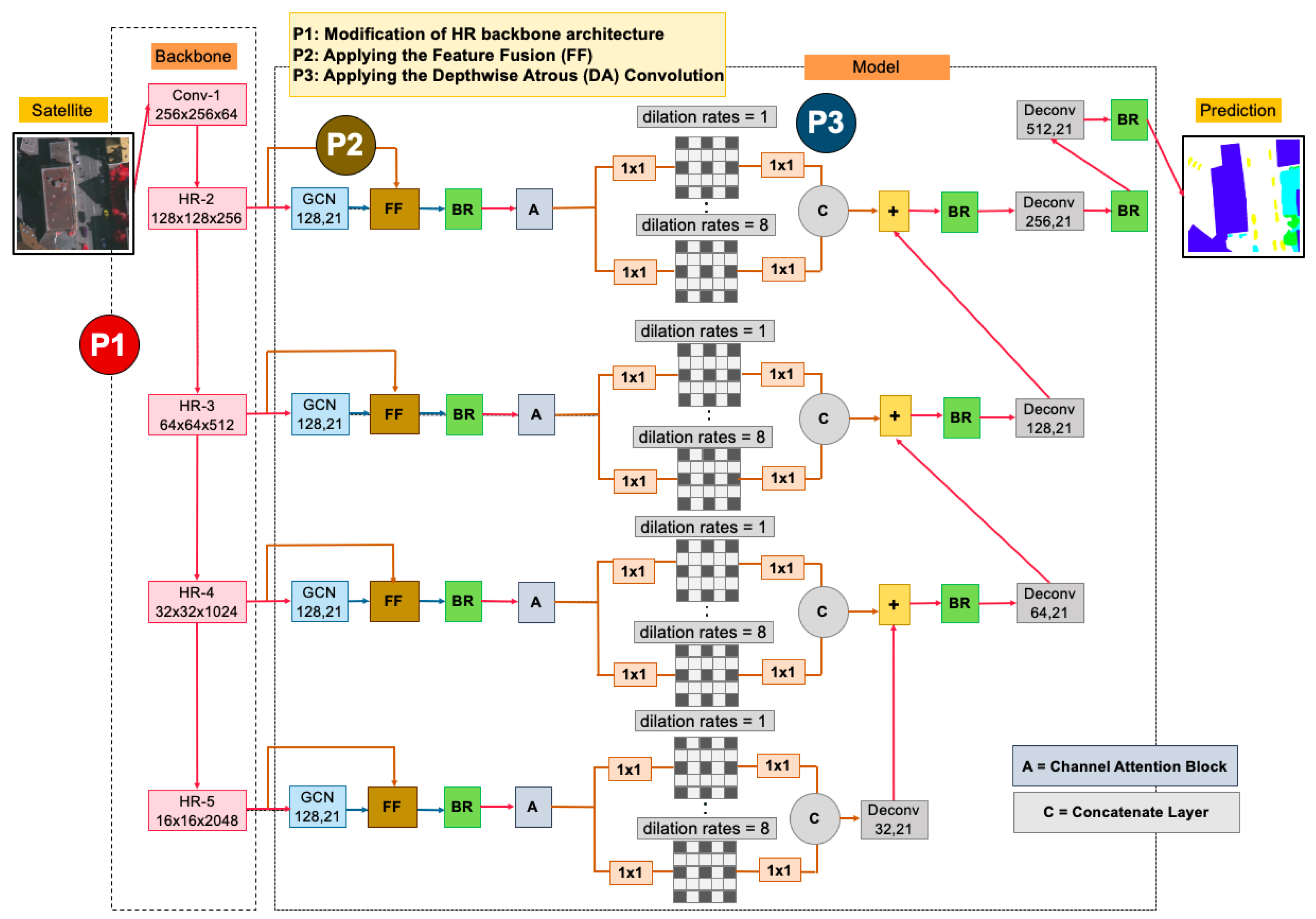
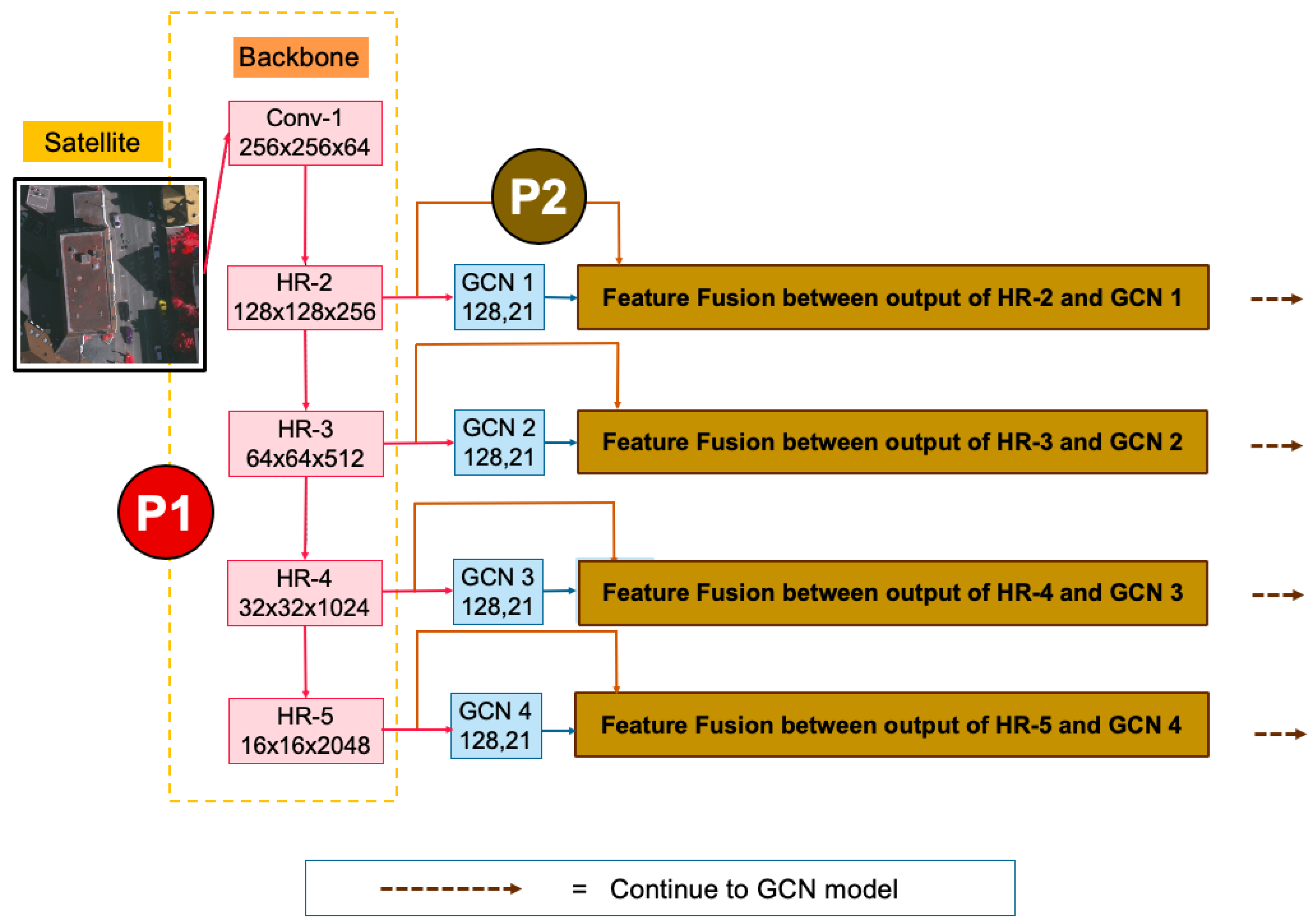
• Proposing the “Feature Fusion (FF)” block into our network to fuse each level feature from the backbone model and the global model of GCN to enrich local and global features.
• Proposing “Depthwise Atrous Convolution (DA)” to bridge the semantic gap and implement durable multi-level feature aggregation to extract complementary information from very shallow features.

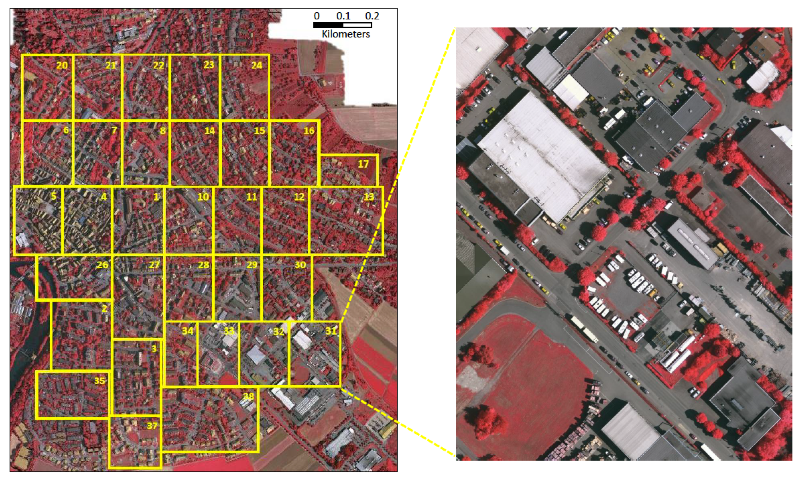
The experiments were conducted using the widespread aerial imagery, ISPRS (Stuttgart) Vaihingen [18] data set and GISTDA (Geo-Informatics and Space Technology Development Agency (Public Organization)), organized by the government in our country, data sets (captured by the Landsat-8 satellite). The results revealed that our proposed method surpasses the two baselines: Deep Convolutional Encoder-Decoder Network (DCED) [19,20,21] and the enhanced Global Convolutional Network (GCN152-TL-A) method [12] in terms of $F1$ score.

The remainder of this paper is organized as follows: Section 2 discusses related work. Our proposed methods are detailed in Section 3. Next, Section 4 provides the details on remote sensing corpora. Section 5 presents our performance evaluation. Then, Section 6 reports the experimental results, and Section 7 is the discussion. Last, we close with the conclusions in Section 8.

2. Related Work

The CNN has been outstandingly utilized for the data analysis of remote sensing domains, in particular, land cover classification or segmentation of agriculture or forest districts [10,12,22,23,24,25,26]. It has rapidly become a successful method for accelerating the process of computer vision tasks, e.g., image classification, object detection, or semantic segmentation with high precision results [4,27,28,29,30,31,32,33] and is a fast-growing area.

It is separated into two subsections: $\left(i\right)$ we demonstrate modern CNN architectures for semantic labeling on both traditional computer vision and remote sensing tasks and $\left(ii\right)$ the novel techniques of deep learning, especially playing with images, are discussed.

2.1. Modern CNN Architecture for Semantic Labeling

In early research, several DCED-based approaches have obtained a high performance in the various baseline corpora [16,19,20,21,26,34,35,36]. Nevertheless, most of them also struggle with issues with performance accuracy. Consequently, much research on novel CNN architectures has been introduced, such as a high-resolution representation [37,38] network that supports high-resolution representations in all processes by connecting high-to-low and low-to-high-resolution convolutions to keep high and low-resolution representations. CSRNet [8] proposed an atrous (dilated) CNN to comprehend highly congested scenes through crowd counting and generating high-quality density maps. They deployed the first ten layers from VGG-16 as the backbone convolutional models and dilated convolution layers as the backend to enlarge receptive fields and extract deeper features without losing resolutions. SeENet [6] enhanced shallow features to alleviate the semantic gap between deep features and shallow features and presented feature attention, which involves discovering complementary information from low-level features to enhance high-level features for precise segmentation. It also was constructed with the parallel pyramid to implement precise semantic segmentation. ExFuse [7] proposed to boost the feature fusion by bridging the semantic and resolution gap between low-level and high-level feature maps. They proposed more semantic information into low-level features with three aspects: $\left(i\right)$ semantic supervision, $\left(ii\right)$ semantic embedding branch, and $\left(iii\right)$ layer rearrangement. They also embeded spatial information into high-level features. In the remote sensing corpus, ResUNet [25] proposed a trustworthy structure for performance effects for the job of image labeling of aerial images. They used a VGG16 network as a backbone, combined with the pyramid scene parsing pooling and dilated deep neural network. They also proposed a new generalized dice loss for semantic segmentation. TreeUNet (also known as adaptive tree convolutional neural networks) [24] proposed a tree-cutting algorithm and an adequate deep neural network with inadequate binary links to increase the classification percentage at the pixel level for subdecimeter aerial imagery segmentation, by sending kernel maps within concatenating connections and fusing multi-scale features. From the ISPRS Vaihingen Challenge and Landsat-8 corpus, the enhanced Global Convolutional Network (also known as “GCN152-TL-A”), illustrated in Figure 1, Panboonyuen et al. (2019) [12] presented an enhanced GCN for semantic labeling with three main contributions. First, “Domain-Specific Transfer Learning” (TL) [13,14,15], illustrated in Figure 2 (right), aims to restate the weights obtained from distinct fields’ inputs. It is currently prevalent in various tasks, such as Natural Language Processing (NLP), and has also become popular in Computer Vision (CV) in the past few years. It allows you to reach a deep learning model with comparatively inadequate data. They prefaced to relieve the lack of issue on the training set by appropriating other remote sensing data sets with various satellites with an essentially pre-trained weight. Next, “Channel Attention”, shown in Figure 2 (left), proposed with their network to select the most discriminative kernels (feature maps). Finally, they enhanced the GCN network by improving its backbone by using “ResNet152”. “GCN152-TL-A” has surpassed state-of-the-art (SOTA) approaches and become the new SOTA. Hence, “GCN152-TL-A” is selected as our baseline in this work.

2.2. Modern Technique of Deep Learning

A novel technique of deep learning is an essential agent for improving the precision of deep learning, especially the CNN. While the most prevalent contemporary designs tick all the boxes for image labeling responsibilities, e.g., the atrous convolution (also known as dilated convolution), channel attention mechanism, refinement residual block, and feature fusion, and have been utilized to boost the performance of the deep learning model.

Atrous convolution [5,6,9,39,40], also known as multi-scale context aggregation, is proposed to regularly aggregate multi-scale contextual information devoid of losing resolution. In this paper, we use the technique of “Depthwise Atrous Convolution (DA)” [6] to extract complementary information from very shallow features and enhance the deep features for improving feature fusion from our feature fusion step.

The channel attention mechanism [16,17] generates a one-dimensional tensor for allowed feature maps, which is activated by the softmax function. It focuses on global features found in some feature maps and has attracted broad interest in extracting rich features in the computer vision domain and offers great potential in improving the performance of the CNN. In previous work, GCN152-TL-A [12], the self attention and utilize channel attention modules are applied to pick the features similar to [16].

Refinement residual block [16] is part of the enhanced CNN model with ResNet-backbones, e.g., ResNet101 or ResNet152. This block is used after the GCN module and during the deconvolution layer. It is used to refine the object boundaries further. In our previous work, GCN152-TL-A [12], we employed the boundary refinement block (BR) that is based on the“Refinement Residual Block” from [11].

Feature fusion [7,41,42,43,44] is regularly manipulated in semantic labeling for different purposes and concepts. It presents a concept that combines multiplied, added, or concatenate CNN layers for improving a process of dimensionality reduction to recover and/or prevent the loss of some important features such as low-level features (e.g., lines, dots, or gradient orientation with the content of an image scene). In another way, it can also recover high-level features by using the technique of “high-to-low and low-to-high” [37,38] to produce high-resolution representations.

3. Proposed Method

Our proposed deep learning architecture, “HR-GCN-FF-DA”, is demonstrated in an overview architecture in Figure 3. The network, based on GCN152-TL-A [12], consists primarily of three parts: (i) changing the backbone architecture (the P1 block in Figure 3), ($ii$) implementing the “Feature Fusion” (the P2 block in Figure 3), and ($iii$) using the concept of “Depthwise Atrous Convolution” (the P3 block in Figure 3).

3.1. Data Preprocessing and Augmentation

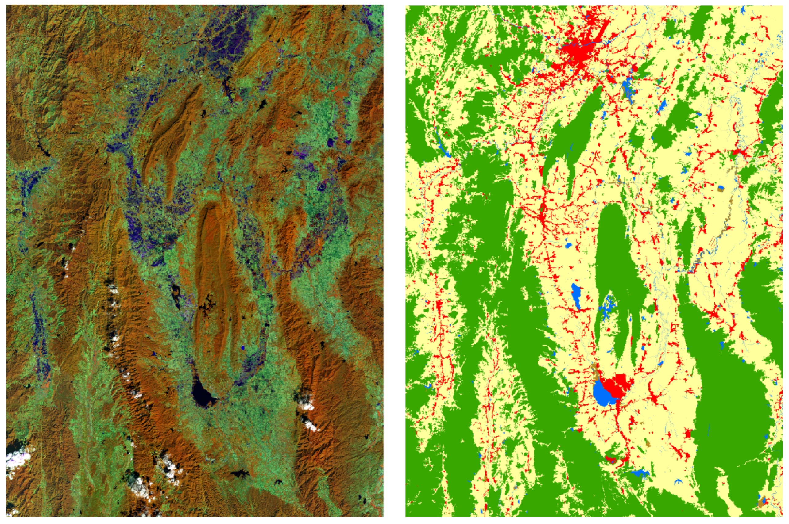
In this work, three benchmarks were used with the experiments, these were the (i) Landsat-8w3c, ($ii$) Landsat-8w5c, and ($iii$) ISPRS Vaihingen (Stuttgart) Challenge data sets. Before a discussion about the model, it is important to deploy a data preprocessing, e.g., pixel standardization, scale pixel values (to have unit variance), and a zero mean into the data sets. In the image domain, the mean subtraction, calculated by the per-channel mean from the training set, is executed in order to improve the model convergence.

Furthermore, a data augmentation (also known as the “ImageDataGenerator” function in TensorFlow/Keras library) is employed, since it can help the model to avoid an overfitting issue and somewhat enlarge the training data—a strategy used to increase the amount of data. To augment the data, each image is width and height-shifted and flipped horizontally and vertically. Then, unwanted outer areas are removed into $512\times 512$ pixels with a resolution of 81 cm${}^2$/pixel in the ISPRS and 900 m${}^2$/pixel in the Landsat-8 data set.

3.2. The GCN with High-Resolution Representations (HR) Front-End

The GCN152-TL-A [12], as shown in Figure 1, is our prior attempt that surpasses a traditional semantic segmentation model, e.g., deep convolutional encoder-decoder (DCED) networks [19,20,21]. By using GCN as our core model, our previous work was improved in three aspects. First, its backbone was revised by varying ResNet-50, ResNet-101, and ResNet-152 networks, as shown in M1 in Figure 1. Second, the “Channel Attention Mechanism” was employed (shown in M2 in Figure 1). Third, the “Domain-Specific Transfer Learning” (TL) was employed to reuse the pre-trained weights obtained from training on other data sets in the remote sensing domain. This strategy is important in the deep learning domain to overcome the limited amount of training data. In our work, there are two main data sets: Landsat-8 and ISPRS. To train the Landsat-8 model, the pre-trained network is obtained by utilizing the ISPRS data. This can also be explained conversely—the pre-trained network can be obtained by Landsat-8 data.

Although the GCN152-TL-A network has determined an encouraging forecast performance, it can still be possible to improve it further through changing the frontend using high-resolution representation (HR) [37,38] instead of ResNet-152 [25,45]. HR has surpassed all existing deep learning methods on semantic segmentation, multi-person pose estimation, object detection, and pose estimation tasks in the COCO, which is large-scale object detection, segmentation, and captioning corpora. It is a parallel structure to enable the deep learning model to link multi-resolution subnetworks in an effective and modern way. HR connects high-to-low subnetworks in parallel. It maintains high-resolution representations through the whole process for a spatially precise heatmap estimation. It creates reliable high-resolution representations through repeatedly fusing the representations generated by the high-to-low subnetworks. It introduces “exchange units” which shuttle across different subnetworks, enabling each one to receive information from other parallel subnetworks. Representations of HR can be obtained by repeating this process. There are four stages as the 2nd, 3rd, 4th, and 5th stages are formed by repeating modularized multi-resolution blocks. A multi-resolution block consists of a multi-resolution group convolution and a multi-resolution convolution, which is illustrated as P1 in Figure 3 (backbone model) and this proposed method is named the “HR-GCN” method.

3.3. Feature Fusion

Inspired by the idea of feature fusion [41,42,43,44] that integrates multiplication, additional, or concatenate layers. Convolution with 1 × 1 filters is used to transform features with different dimensions into the shape, which can be fused. The fusion method contains an addition process. Each layer of the backbone network such as VGG, Inception, ResNet, or HR creates the feature map for specific. We proposed to combine output with low-level features (front-end network) with the deep model and refine the feature information.

As shown in Figure 4, the kernel maps after fusing will be calculated as Equation (1):

$$Z_{add}=X_1\oplus X_2\oplus X_3···\oplus X_i···\oplus X_j$$

(1)

where j adverts to the index of the layer, $X_k$ is a set of output activation maps of one layer and ⊕ adverts to element-wise addition.

Hence, the nature of the addition process encourages essential information to build classifiers to comprehend the feature details. It denotes all bands of $Z_{add}$ to hold more feature information.

Equation (2) shows the relationship between input and output. Thus, we take the fusion activation map into the model again, it can be performed as Equation (4):

$${\overline{y}}^i=ReLU(w^T{x}^i+b)$$

(2)

where x is the input and output of layer of the convolution recorded as $y^i$; b and w refer to bias and weight. The cost function in this work is demonstrated via Equation (3).

$$J(w,b)=-\frac{1}{m}\times \left[(1-y^{\left(i\right)})log\right(1-{\overline{y}}^{\left(i\right)}+\left(y^{\left(i\right)}log\left({\overline{y}}^{\left(i\right)}\right)\right]$$

(3)

where y refers to segmentation target of input (each image) and J, w, and b are the loss, weight, and bias value, respectively.

$$Y_{add}=f(W_k{Z}_{add}+B_k)$$

(4)

The feature fusion procedure always transforms into the same thing when using additional procedures. In this work, we use addition fusion elements, as shown in Figure 4.

3.4. Depthwise Atrous Convolution (DA)

Depthwise Atrous Convolution (DA) [6,9,39] is presented to settle the contradictory requirements between the larger region of the input space that affects a particular unit of the deep network (receptive fields) and activation map resolution.

DA is a robust operation to reduce the number of parameters (weights) in the layer of the CNN while maintaining a similar performance that includes the computation cost and tunes the kernel’s field-of-view in order to capture a generalized standard convolution operation and multi-scale information. An atrous filter can be a dilated kernel in varied rates, e.g., rate = 1, 2, 4, 8, by inserting zeros into appropriate positions in the kernel mask.

Basically, the DA module uses atrous convolutions to aggregate multi-scale contextual information without dissipating resolution orderly in each layer. It generalizes “Kronecker-factored” convolutional kernels, and it allows for broad receptive fields, while only expanding the number of weights logarithmically. In other words, DA can apply the same kernel at distinct scales using various atrous factors.

Compared to the ordinary convolution operator, atrous (dilated) convolution is able to achieve a larger receptive field size without increasing the numbers of kernel parameters.

Our motivation is to apply DA to solve challenging scale variations and to trade off precision in aerial and satellite images, as shown in Figure 5.

In a one-dimensional (1D) case, let $x\left[i\right]$ denote input signal, and $y\left[i\right]$ denote output signal. The dilated convolution is formulated as Equation (5):

$$y\left[i\right]=\sum _{j=1}^{J}x[i+a·k]·w\left[j\right]$$

(5)

where a is the atrous (dilated) rate, $w\left[j\right]$ denotes the j-th parameter of the kernel, and J is the filter size. This equation reduces to a standard convolution when d = 1, 2, 4, and 8, respectively.

In the cascading mode from DeepLabV3 [46,47] and Atrous Spatial Pyramid Pooling (ASPP) [9], multi-scale contextual information can be encoded by probing the incoming features with dilated convolution to capture sharper object boundaries by continuously recovering the spatial characteristic. DA has been applied to increase the computational ability and achieve the performance by factorizing a traditional convolution into a depth-wise convolution followed by a point-wise convolution, such as $1\times 1$ convolution (it is often applied on the low-level attributes to decrease the whole of the bands (kernel maps)).

To simplify notations, $H_{J,a}\left(x\right)$ is term of a dilated convolution, and ASPP can be performed as Equation (6).

$$y=H_{3,1}\left(x\right)+H_{3,2}\left(x\right)+H_{3,4}\left(x\right)+H_{3,8}\left(x\right)$$

(6)

To improve the semantics of shallow features, we apply the idea of multiple dilated convolution with different sampling rates to the input kernel map before continuing with the decoder network and adjusting the dilation rates (1, 2, 4, and 8) to configure the whole process of our proposed method called “HR-GCN-FF-DA”, shown in P3 in Figure 3 and Figure 5.

4. Remote Sensing Corpora

In our experiments, there are two main sources of data: public and private corpora. The private corpora is the medium resolution imagery received from the satellite “Landsat-8” used by the government organization in Thailand called GISTDA. Since there are two variations of annotations, the Landsat-8 data is considered as two data sets: one with three classes and the other with five classes, as shown in

Table 1. Abbreviations on our Landsat-8 corpora.

Abbreviation	Description
Landsat-8w3c corpus	Landsat-8 corpus with 3 classes
Landsat-8w5c corpus	Landsat-8 corpus with 5 classes

. The public corpora is very high-resolution imagery from the standard benchmark called “ISPRS Vaihingen (Stuttgart)”. Evaluations based on classification/segmentation metrics, e.g., $F1Score$, $Precision$, $Recall$ and $AverageAccuracy$ are deployed with all experiments.

4.1. Landsat-8w3c Corpus

For this corpus, there is a new benchmark that differs from our previous work. All images are taken in the area of the northern provinces (Changwat) of Thailand. The data set is made from the Landsat-8 satellite consisting of 1420 satellite images, some samples are shown in Figure 6. This data set contains a massive collection of medium resolution imagery of (20,921 × 17,472) pixels. There are three classes: para rubber (red), pineapple (green), and corn (yellow). From a total of 1390 images, the images are separated into 1000 training and 230 validation images, as well as 190 test images to compare with other baseline methods.

4.2. Landsat-8w5c Corpus

This data set is the same corpus from Landsat-8, but it is annotated with five class labels: agriculture, forest, miscellaneous (misc), urban, and water as shown in Figure 7. There are 1012 medium resolution satellite images of 17,200 × 16,300 pixels. From the total 1039 images, the images are separated into 700 training and 239 validation images, as well as 100 test images to comparison to other baseline methods.

4.3. ISPRS Vaihingen Corpus

The challenge of ISPRS semantic segmentation at Vaihingen (Stuttgart) [18] (Figure 8 and Figure 9) is used to be our standard corpus. They were captured over Vaihingen in Germany. The data set is a subset of the data used for the test of digital aerial cameras carried out by the German Association of Photogrammetry and Remote Sensing (DGPF).

It consists of three spectral bands such as NDSM, DSM, near-infrared bands, red, and green data. For our work, NDSM and DSM data are not used in this corpus. They provide 33 images of about 2500 × 2000 pixels of about 9 cm of resolution. Following other methods, four scenes such as scene 5, 7, 23, and 30 are removed from the training set as a validation set. All experimental results are announced on the validation set if not specified.

5. Performance Evaluation

The performance of “HR-GCN-FF-DA” is evaluated in all corpora for $F1$ and $AverageAccuracy$. To assess class-specific performance, the $F1$, $precision$, $recall$, and $AverageAccuracy$ metric are used. It is computed as the symphonious average between recall and precision. We carry $precision$, $recall$, and $F1$ as fundamental metrics and also incorporate the $AverageAccuracy$, which calculates the number of correctly classified positions and divides it by the total number of the reference positions. The $AverageAccuracy$ and $F1$ metrics can be assessed using Equations (7)–(10).

The confusion matrix for pixel-level classification [18] and the false positive (denoted as FP) are computed from the summation of the column. In contrast, the false negative (denoted as FN) is the summation of the horizontal axis, excluding the principal diagonal factor. Next, the true positive (denoted as TP) is the value of the identical oblique elements, and the true negative (denote as TN) contrasts TP.

$$Precision=\frac{TP}{TP+FP}$$

(7)

$$Recall=\frac{TP}{TP+FN}$$

(8)

$$F1=\frac{2\times Precision\times Recall}{Precison+Recall}$$

(9)

$$AverageAccuracy=\frac{TP+TN}{TP++FP+FN+TN}$$

(10)

6. Experimental Results

For a python deep learning framework, we use “Tensorflow (TF)” [48], an end-to-end open source platform for deep learning. The whole experiment was implemented on servers with Intel^® 2066 core I9-10900X, 128 GB of memory, and the NVIDIA RTX™ 2080Ti (11 GB) x 4 cards.

For the training phrase, the adaptive learning rate optimization algorithm (extension to the stochastic gradient descent (SGD)) [49] and batch normalization [50], a technique for improving the performance, stability, and speed of deep learning, were applied and standardized to ease the training in every experiment.

For the learning rate schedules tasks, [9,16,32], we selected the polylearning rate policy. As shown in Equation (11), the learning rate is scheduled by multiplying a decaying factor to the initial learning rate (4 × 10${}^{-3}$).

$$learningrate=init\_learningrate\times {(1-\frac{epoch}{MaxEpoch})}^{0.9}$$

(11)

All deep CNN models are trained for 30 epochs on the Landsat-8w3c corpus and ISPRS Vaihingen data sets. It is increased to be 50 epochs for the Landsat-8w5c data set. Each image is resized to $521\times 521$ pixels along with augmented data using a randomly cropping strategy. Weights are updated using the mini-batch of 4.

This section explains the elements of our experiments. The proposed CNN architecture is based on the victor from our previous work called “GCN152-TL-A” [12]. In our work, there are three proposed improvements: (i) adjusting backbones using high-resolution representations, ($ii$) the feature fusion module, and ($iii$) depthwise atrous convolution. From all proposed policies, there are four acronyms of procedures, as shown in

Table 2. Acronyms of our proposed deep learning approaches.

Acronym	Representation
A	Channel Attention Block
DA	Depthwise Atrous Convolution
FF	Feature Fusion
HR	High-Resolution Representations

.

There are three subsections to discuss the experimental results of each data set: (i) Landsat-8w3c, ($ii$) Landsat-8w5c, and ($iii$) ISPRS Vaihingen data sets.

There are two baseline models of the semantic labeling task in the domains of remote sensing-based information on the computer vision. The first baseline is DCED, which is commonly used in much segmentation work [19,20,21]. The second baseline is the winner of our previous work called “GCN152-A-TL” [12]. Note that “GCN-A-TL” is abbreviated using just “GCN”, since we always employ the attention and transfer-learning strategies into our proposed models.

Each proposed tactic can elevate the completion of the baseline approach shown via the whole experiment. First, the effect of our new backbone (HRNET) is investigated by using HRNET on the GCN framework called “HR-GCN”. Second, the effect of our feature fusion is shown by adding it into our model, called “HR-GCN-FF”. Third, the effect of the depthwise atrous convolution is explained by using it on top of a traditional convolution mechanism, called “HR-GCN-FF-DA”.

6.1. The Results of Landsat-8w3c Data Set

The Landsat-8w3c corpus was used in all experiments. We distinguished between the alterations of the proposed approaches and CNN baselines. “HR-GCN-FF-DA”, the full proposed method, is the winner with $F1$ of 0.9114. Furthermore, it is also the winner of all classes. More detailed results are given in the next subsection. Presented in

Table 3. Effects on the testing set of the Landsat-8w3c data set.

	Pretrained	Frontend	Model	$\mathit{Precision}$	$\mathit{Recall}$	$\mathit{F}1$
Baseline	-	VGG16	DCED [19,20,21]	0.8546	0.7723	0.8114
	TL	Res152	GCN-A [12]	0.8732	0.8722	0.8727
Proposed Method	TL	HRNET	GCN-A	0.8693	0.8836	0.8764
	TL	HRNET	GCN-A-FF	0.8797	0.8910	0.8853
	TL	HRNET	GCN-A-FF-DA	0.8999	0.9233	0.9114

and

Table 4. Effects on the testing set of the Landsat-8w3c data set among each class with our proposed procedures in terms of $AverageAccuracy$.

	Model	Para Rubber	Pineapple	Corn
Baseline	DCED [19,20,21]	0.8218	0.8618	0.8084
	GCN152-TL-A [12]	0.9127	0.7778	0.8878
Proposed Method	HR-GCN	0.8371	0.8147	0.8621
	HR-GCN-FF	0.9179	0.8689	0.8989
	HR-GCN-FF-DA	0.9386	0.8881	0.9184

are the results of this corpus, Landsat-8w3c.

6.1.1. HR-GCN Model: Effect of Heightened GCN with High-Resolution Representations on Landsat-8w3c

The previous enhanced GCN network is improved to increase the $F1$ score by using the High-Resolution Representations (HR) backbone instead of the ResNet-152 backbone (best frontend network from our previous work). $F1$ of HR-GCN (0.8763) outperforms that of the baseline methods. DCED (0.8114) and GCN152-TL-A (0.8727) refer to Table 3 and Table 4. The result returns a higher $F1$ at 6.50% and 0.36%, respectively. Hence, it means the features extracted from HRNET are better than those from ResNet-152.

For the analysis of each class, HR-GCN achieved an average accuracy on para rubber, pineapple, and corn for 0.8371, 0.8147, and 0.8621, consecutively. Compared to DCED, it won in two classes: para rubber and corn. However, it won against our previous work (GCN152-TL-A) only in the pineapple class.

6.1.2. HR-GCN-FF Model: Effect of Using “Feature Fusion” on Landsat-8w3c

Next, we apply “Feature Fusion” to capture low-level features to decorate the feature information of CNN. HR-GCN-FF (0.8852) is higher than that of HR-GCN (0.8763), GCN152-TL-A (0.8727), and DCED (0.8113), shown in Table 3 and Table 4. It gives a higher $F1$ score at 0.89%, 1.26%, and 7.39%, consecutively.

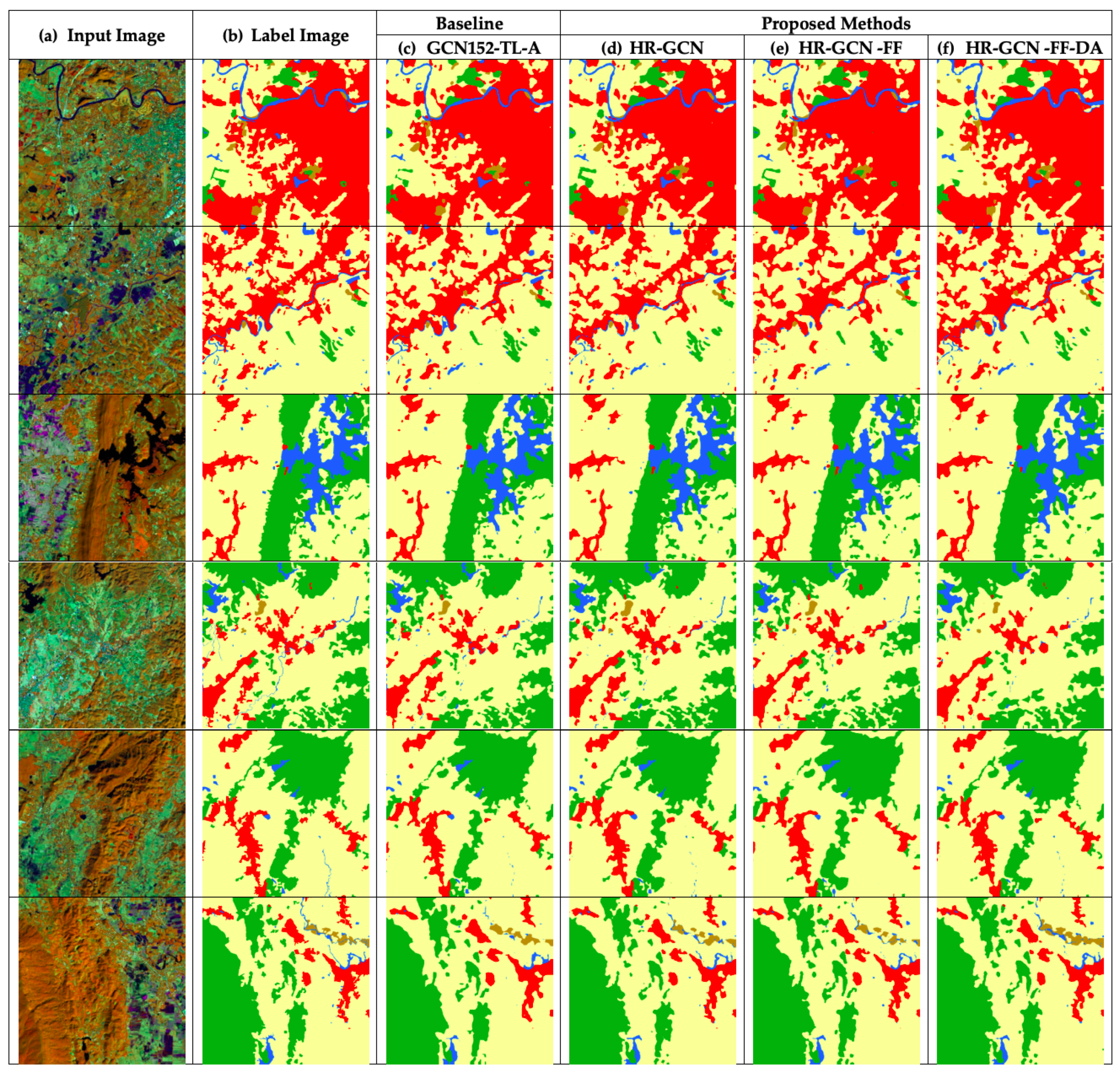
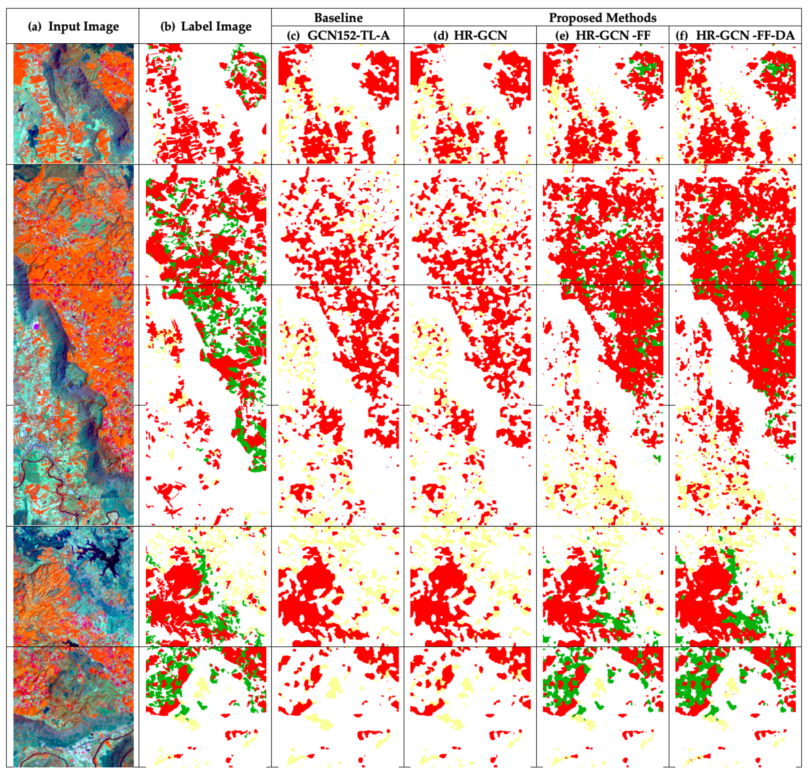
It is interesting that the FF module can really improve the performance in all classes, especially in the para rubber and pineapple classes. It outperforms both HR-GCN and all baselines in all classes. To further investigate the results, Figure 10e and Figure 11e show that the model with FF can capture pineapple (green area) surrounded in para rubber (red area).

6.1.3. HR-GCN-FF-DA Model: Effect of Using “Depthwise Atrous Convolution” on Landsat-8w3c

The last strategy aims to use an approach of “Depthwise Atrous Convolution” (details in Section 3.4) by extracting complementary information from very shallow features and enhancing the deep features for improving feature fusion of the Landsat-8w3c corpus. The “HR-GCN-FF-DA” method is the victor. $F1$ is obviously more distinguished than DCED at 10.00% and GCN152-TL-A (the best benchmark) at 3.87%, as shown in Table 3 and Table 4.

For an analysis of each class, our model is clearly the winner in all classes with an accuracy beyond 90% in two classes: para rubber and corn. Figure 10 and Figure 11 show twelve sample outputs from our proposed methods (column $\left(dtof\right)$) compared to the baseline (column $\left(c\right)$) to expose improvements in its results. From our investigation, we found that the dilated convolutional concept can make our model have better overview information, so it can capture larger areas of data.

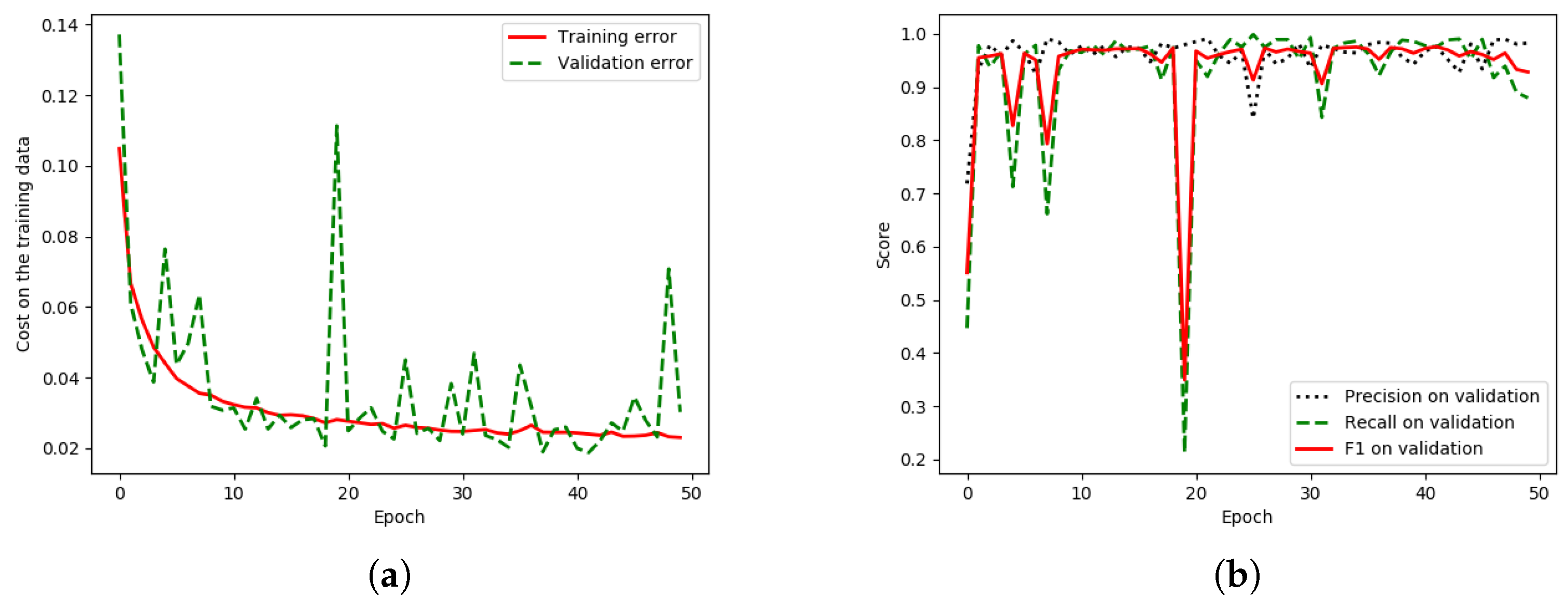
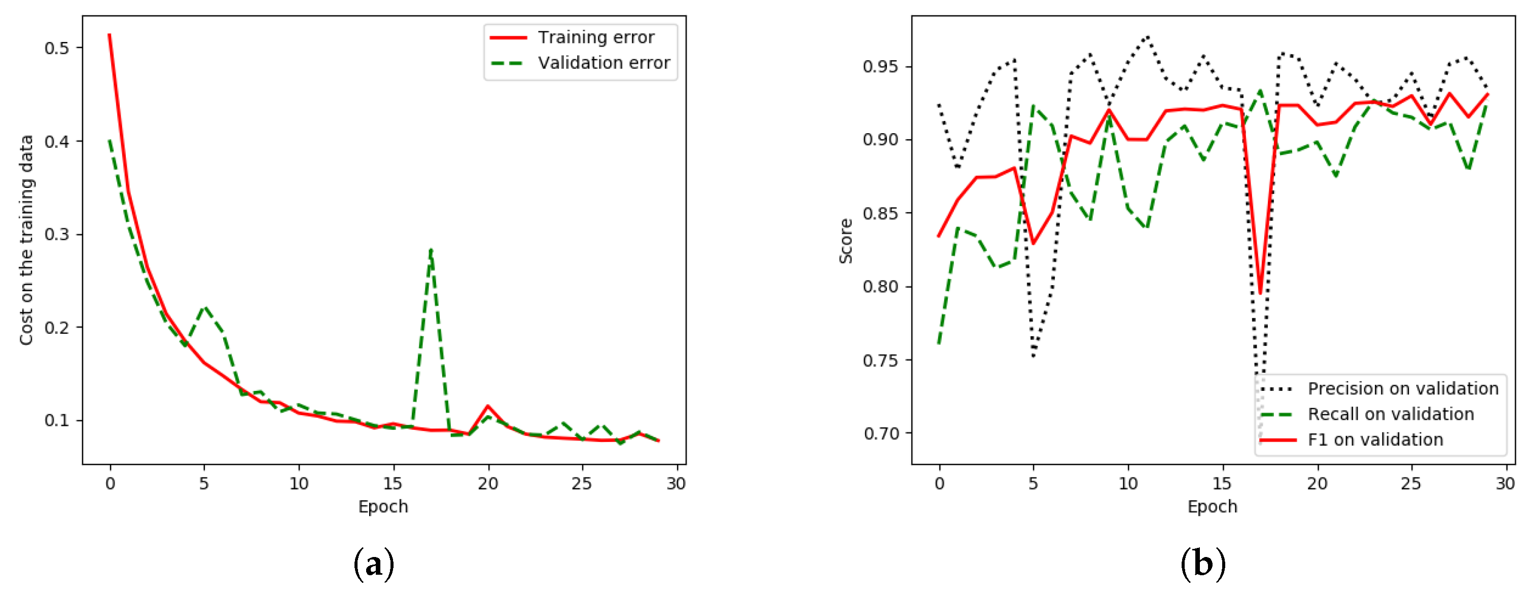
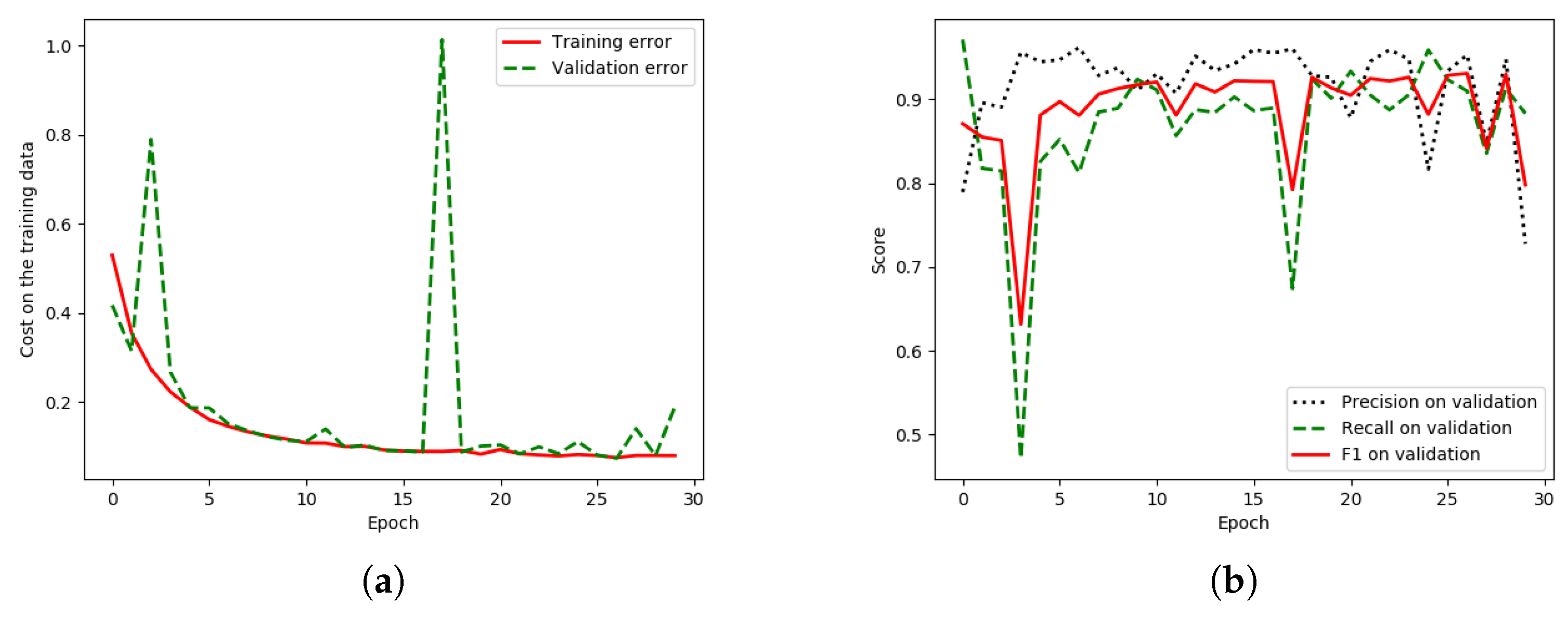
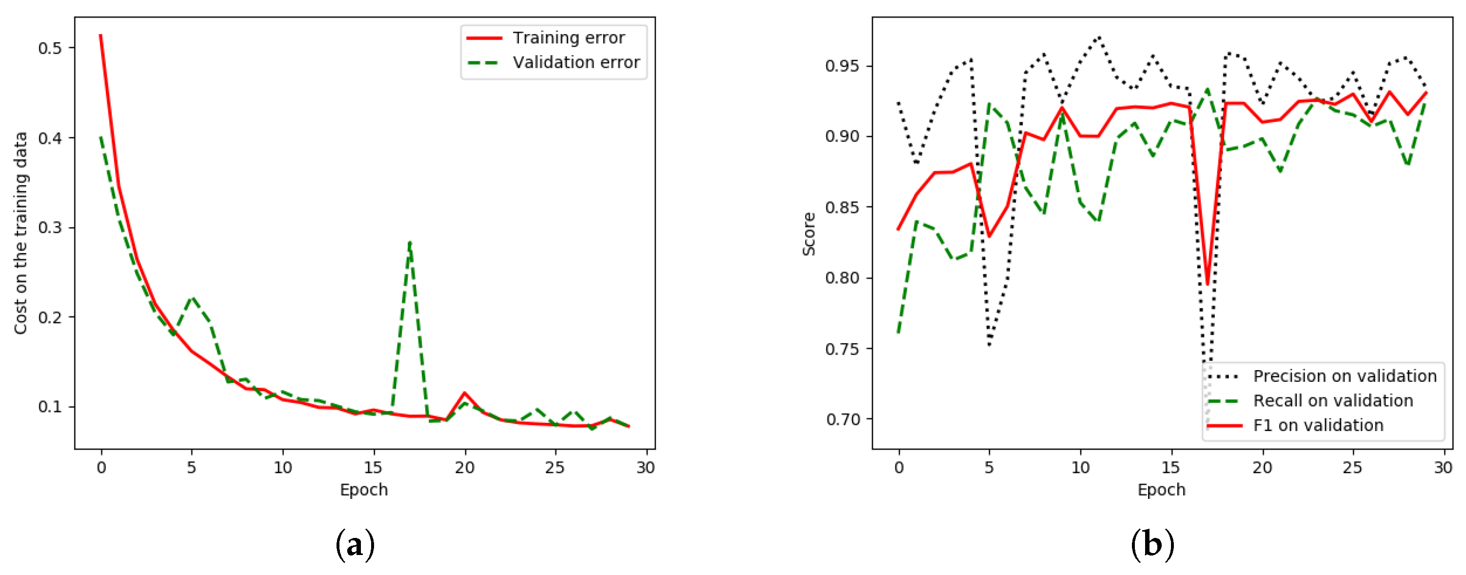
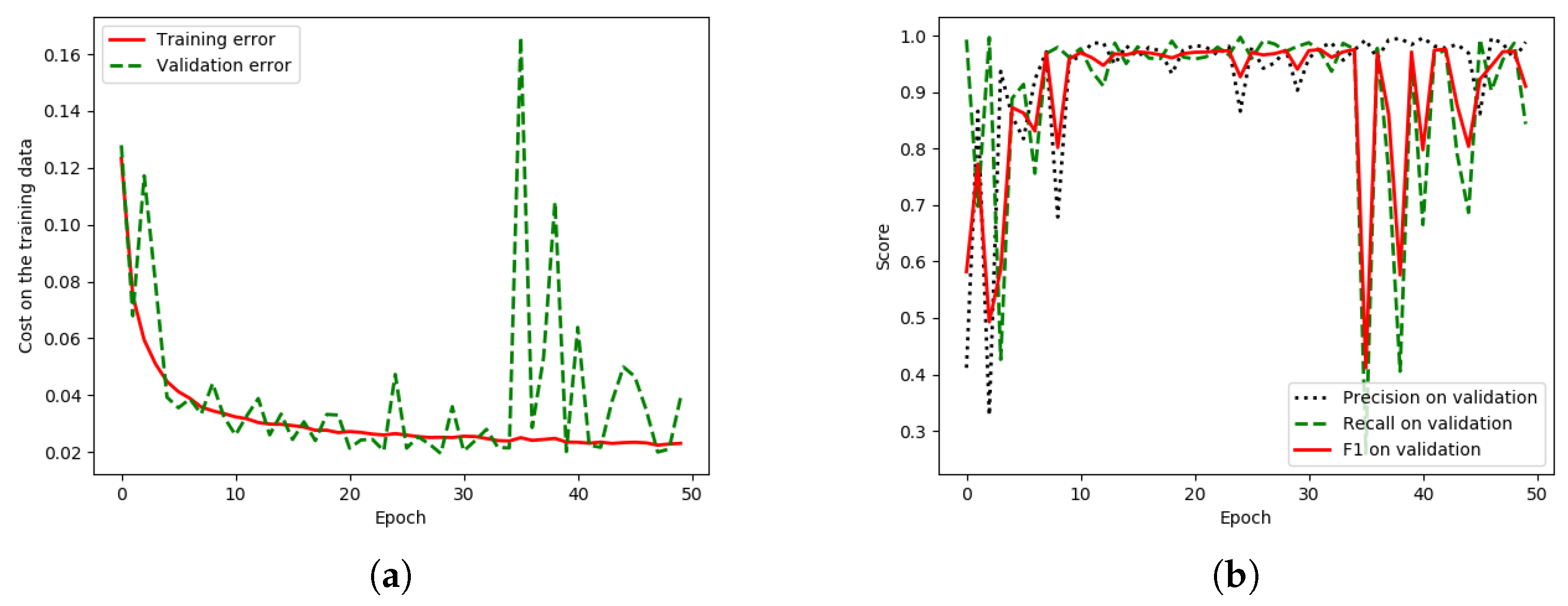
There is a lower discrepancy (peak) in the validation data of “HR-GCN-FF-DA”, Figure 12a, than that in the baseline, Figure 13a. Moreover, Figure 13b and Figure 12b show three learning graphs such as precision, recall, and F1 lines. The loss graph of the “HR-GCN-FF-DA” model seems flatter (very smooth) than the baseline in Figure 13a. The epoch at number 27 was selected to be a pre-trained model for testing and transfer learning procedures.

6.2. The Results on Landsat-8w5c Data Set

In this subsection, the Landsat-8w5c corpus was conducted on all experiments. We compare “HR-GCN-FF-DA” network (column $\left(f\right)$) to CNN baselines via

Table 5. Effects on the testing set of Landsat-8w5c data set.

	Pre-trained	Frontend	Model	$\mathit{Precision}$	$\mathit{Recall}$	$\mathit{F}1$
Baseline	-	VGG16	DCED [19,20,21]	0.8571	0.8441	0.8506
	TL	Res152	GCN-A [12]	0.8616	0.8973	0.8791
Proposed Method	TL	HRNET	GCN-A	0.8918	0.8877	0.8898
	TL	HRNET	GCN-A-FF	0.9209	0.9181	0.9195
	TL	HRNET	GCN-A-FF-DA	0.9338	0.9385	0.9362

and

Table 6. Effects on the testing set of Landsat-8w5c data set among each class with our proposed procedures in terms of $AverageAccuracy$.

	Model	Agriculture	Forest	Misc	Urban	Water
Baseline	DCED [19,20,21]	0.9819	0.9619	0.7628	0.8538	0.7250
	GCN152-TL-A [12]	0.9757	0.9294	0.6847	0.9288	0.7846
Proposed Method	HR-GCN	0.9755	0.9501	0.8231	0.9133	0.7972
	HR-GCN-FF	0.9741	0.9526	0.8641	0.9335	0.8282
	HR-GCN-FF-DA	0.9856	0.9531	0.9176	0.9561	0.8437

. “HR-GCN-FF-DA” is the winner with a $F1$ of 0.9111. Furthermore, it is also the winner in all classes especially water and urban class that are composed with low-level features. More detailed results are described in the next subsection and are presented in Table 5 and Table 6 for the results of this data set, Landsat-8w5c.

6.2.1. HR-GCN Model: Effect of Heightened GCN with High-Resolution Representations on Landsat-8w5c

The $F1$ score of HR-GCN (0.8897) outperforms that of baseline methods: DCED (0.8505) and GCN152-TL-A (0.8791); $F1$ at 3.92% and 1.07% respectively. The main reason is due to both higher recall and precision. This can imply that features extracted from HRNET are also better than those from ResNet-152 on Landsat-8 images as well, shown in Table 5 and Table 6.

For the analysis on each class, HR-GCN achieved an averaging accuracy in agriculture, forest, miscellaneous, urban, and water for 0.9755, 0.9501, 0.8231, 0.9133, and 0.7972, consecutively. Compared to DCED, it won in three classes: forest, miscellaneous and water. However, it won against our previous work (GCN152-TL-A) in the pineapple class, and it showed about the same performance in the agriculture class.

6.2.2. HR-GCN-FF Model: Effect of Using “Feature Fusion” on Landsat-8w5c

The second mechanism focuses on utilizing ‘Feature Fusion” to fuse each level feature for enriching the feature information. From Table 5 and Table 6, the $F1$ of HR-GCN-FF (0.9195) is greater than that of HR-GCN (0.8897), GCN152-TL-A (0.8791), and DCED (0.8505). It produces a more precise $F1$ score at 2.97%, 4.04%, and 6.89%.

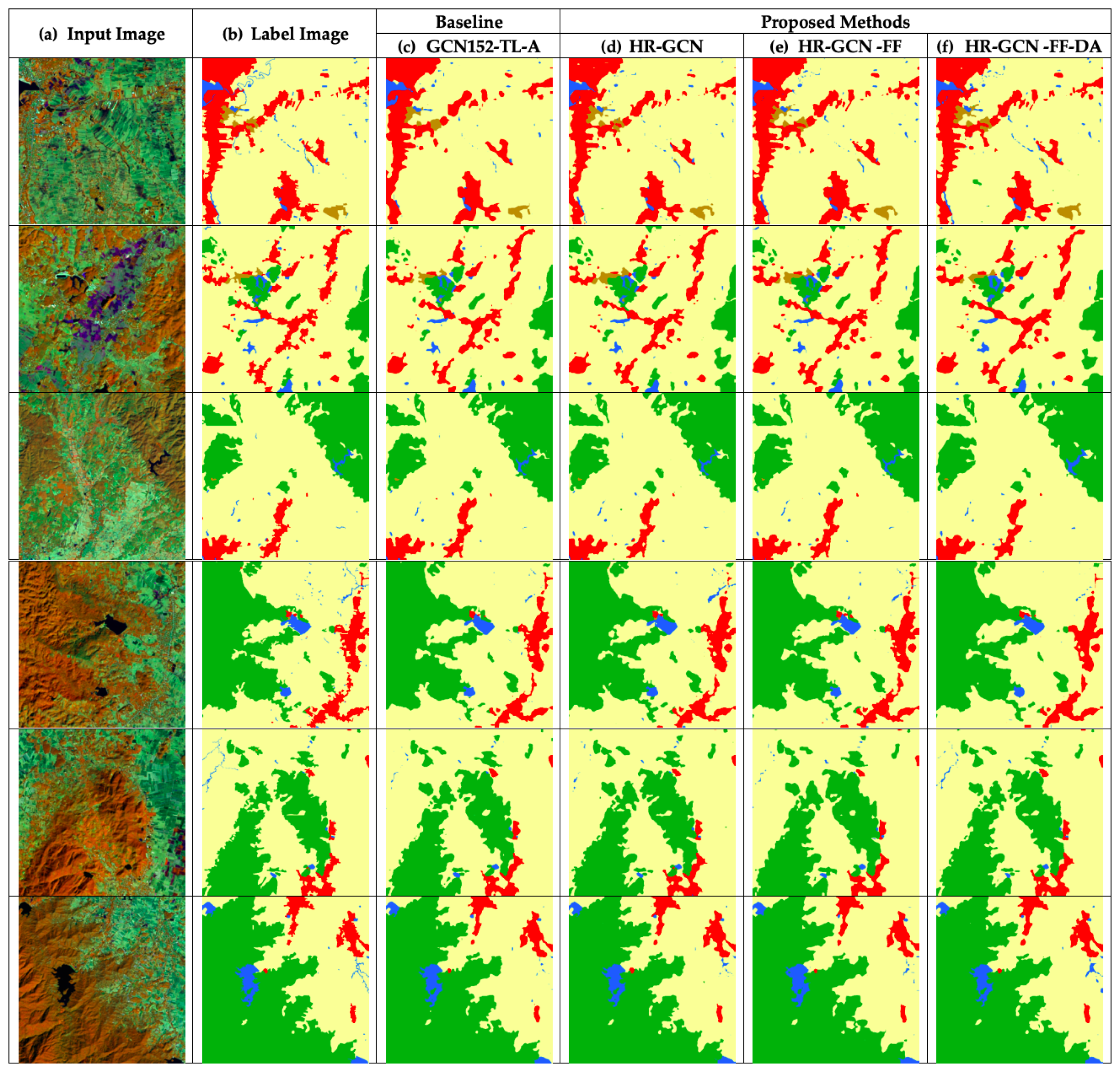
To further analyze the results, Figure 14e and Figure 15e show that the FF module can better capture low-level details. Especially in the water class, it can recover the missing water area, resulting in an improvement of accuracy from 0.7972 to 0.8282 (3.1%).

6.2.3. HR-GCN-FF-DA Model: Effect of Using “Depthwise Atrous Convolution” on Landsat-8w5c

The last policy points to the performance of the method of “Depthwise Atrous Convolution” by enhancing the features of CNN for improving the previous step. The $F1$ score of the “HR-GCN-FF-DA” approach is the conqueror. It is more eminent than DCED and GCN152-TL at 8.56% and 5.71%, consecutively, shown in Table 5 and Table 6.

In the dilated convolution, filters are boarder, which can capture better overview details resulting in (i) larger coverage areas and ($ii$) connected small areas together.

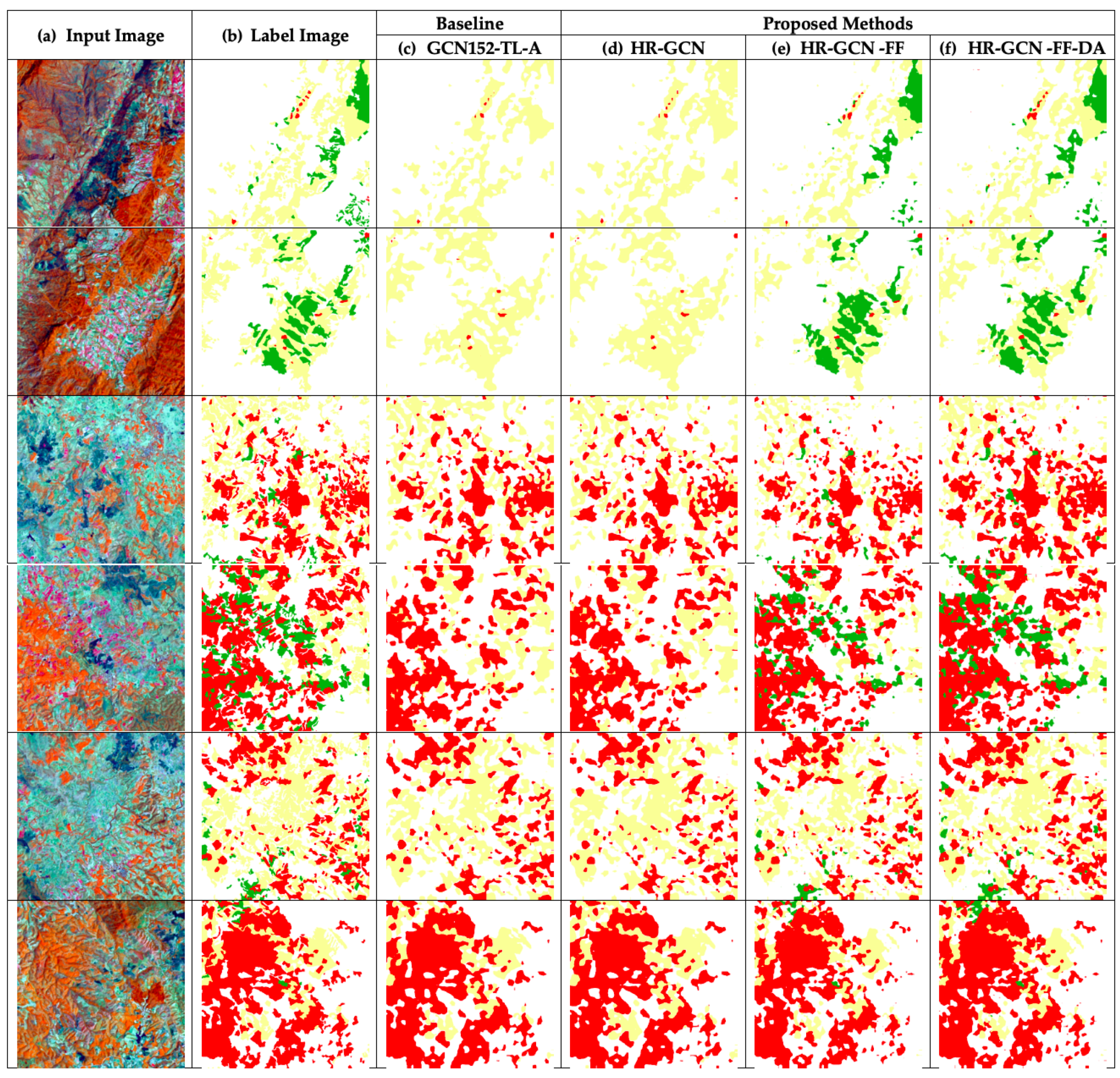
For an analysis of each class, our final model is clearly the winner in all classes with an accuracy beyond 95% in two classes: agriculture and urban classes. Figure 14 and Figure 15 show twelve sample outputs from our proposed methods (column $\left(dtof\right)$) compared to the baseline (column $\left(c\right)$) to expose improvements in its results and that founds that Figure 14f and Figure 15f are likewise to the ground images. From our investigation, we found that the dilated convolutional concept can make our model have better overview information, so it can capture larger areas of data.

Considering the loss graphs, our model in Figure 16a can learn smoother than the baseline (our previous work) in Figure 17a, since the discrepancy (peak) in the validation error (green line) is lower in our model. There is a lower discrepancy (peak) in the validation data of “HR-GCN-FF-DA”, Figure 16a, than that in the baseline, Figure 17a. Moreover, Figure 17b and Figure 16b show three learning graphs such as precision, recall, and F1 lines. The loss graph of the “HR-GCN-FF-DA” model seems flatter (very smooth) than the baseline in Figure 17a and the epoch at number 40 out of 50 was selected to be a pre-trained model for testing and transfer learning procedures.

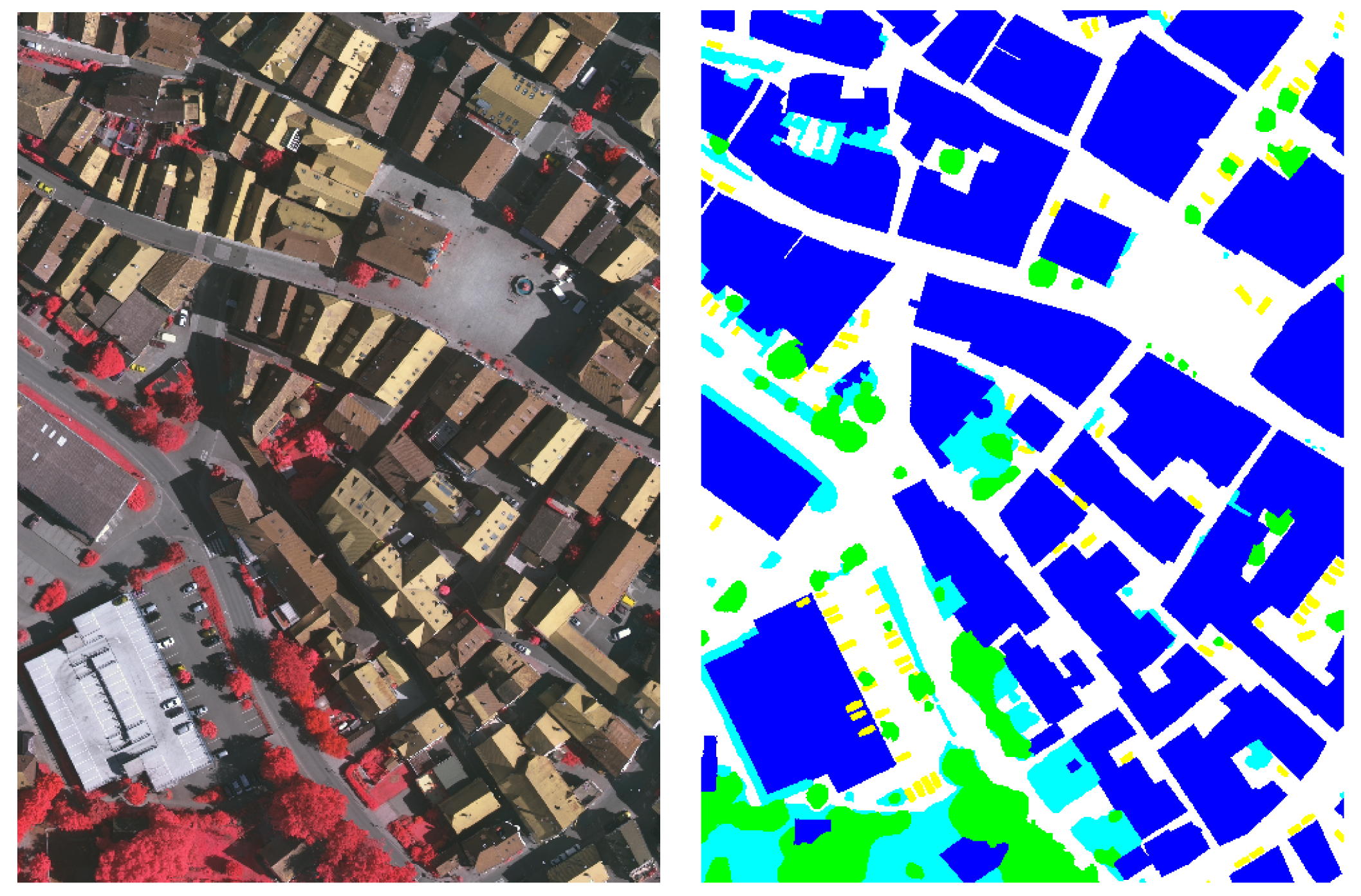
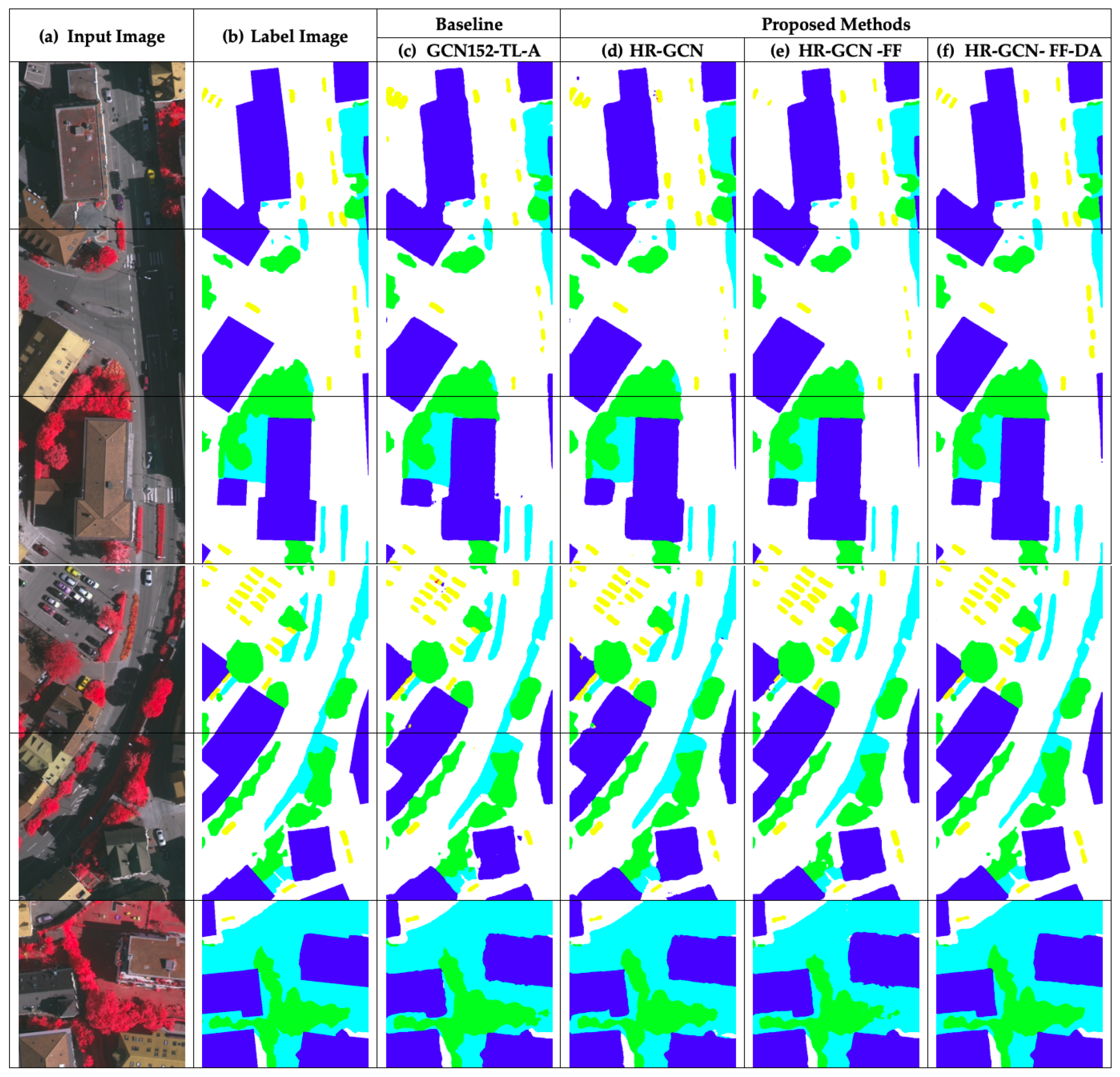
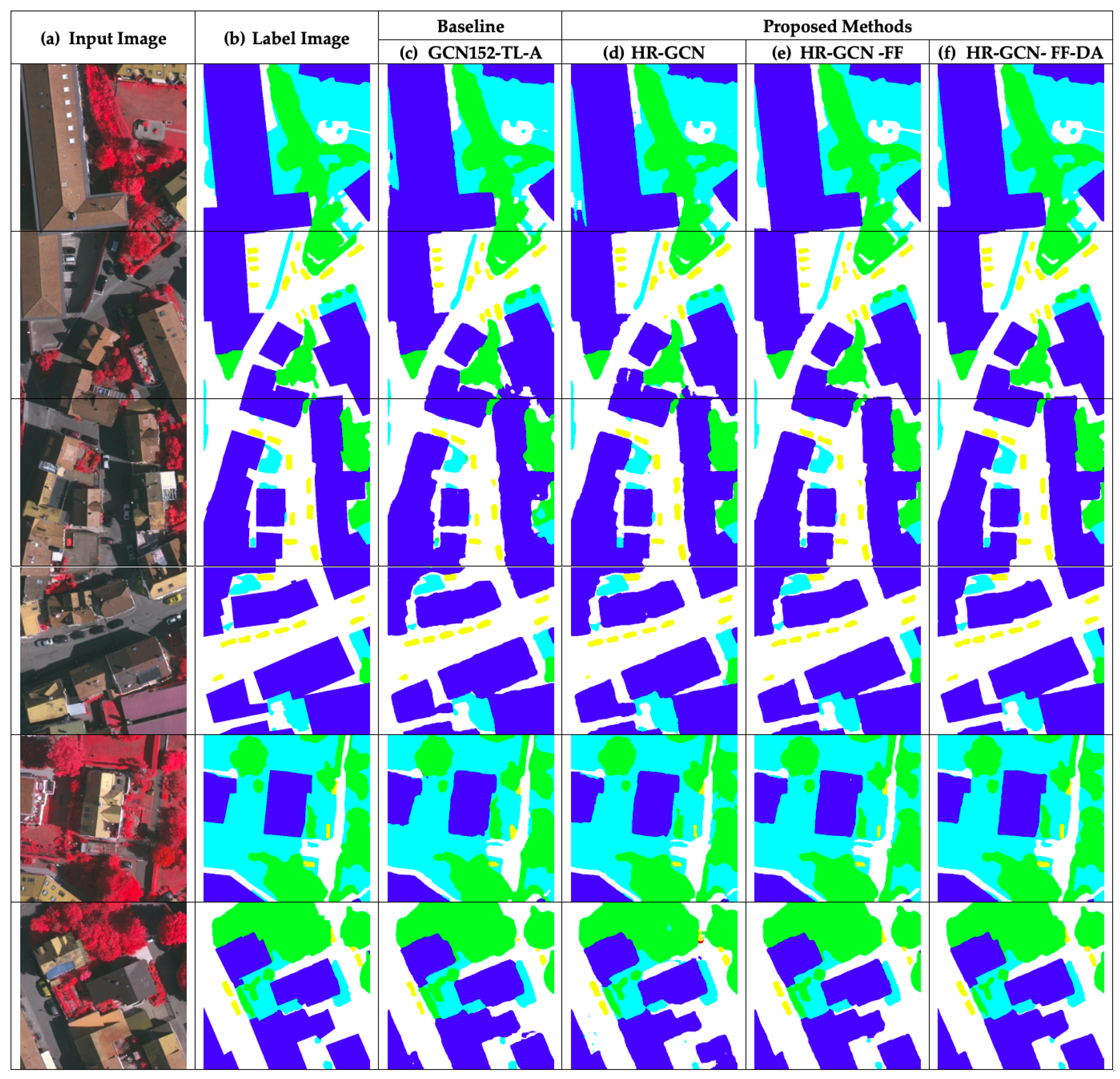
6.3. The Results in ISPRS Vaihingen Challenge Data Set

In this subsection, the ISPRS Vaihingen (Stuttgart) Challenge corpus was used in all experiments. The “HR-GCN-FF-DA” is the winner with $F1$ of 0.9111. Furthermore, it is also the winner of all classes. More detailed results will be provided in the next subsection, and the consequences of our proposed method with CNN baselines for this data set are shown in

Table 7. Effects on the testing set of ISPRS Vaihingen (Stuttgart) challenge data set.

	Pre-trained	Frontend	Model	$\mathit{Precision}$	$\mathit{Recall}$	$\mathit{F}1$
Baseline	-	VGG16	DCED [19,20,21]	0.8672	0.8490	0.8580
	TL	Res152	GCN-A [12]	0.8724	0.8520	0.8620
Proposed Method	TL	HRNET	GCN-A	0.8717	0.8686	0.8701
	TL	HRNET	GCN-A-FF	0.8981	0.8812	0.8896
	TL	HRNET	GCN-A-FF-DA	0.9228	0.8997	0.9111

and

Table 8. Effects on the testing set of ISPRS Vaihingen (Stuttgart) challenge data set among each class with our proposed procedures in terms of $AverageAccuracy$.

	Model	IS	Buildings	LV	Tree	Car
Baseline	DCED [19,20,21]	0.8721	0.8932	0.8410	0.9144	0.8153
	GCN152-TL-A [12]	0.8758	0.8725	0.8567	0.9534	0.8034
Proposed Method	HR-GCN	0.8864	0.9282	0.8114	0.8945	0.8202
	HR-GCN-FF	0.8279	0.9458	0.9264	0.9475	0.8502
	HR-GCN-FF-DA	0.9075	0.9589	0.9266	0.9299	0.8710

.

6.3.1. HR-GCN Model: Effect of Heightened GCN with High-Resolution Representations in ISPRS Vaihingen

The $F1$ score of HR-GCN (0.8701) exceeds that of the baseline methods: DCED (0.8580) and GCN152-TL-A (0.8620). It complies a higher $F1$ at 1.21% and 0.81%, respectively. This shows that the enhanced GCN with HR backbone is also more significantly streamlined than the GCN152-TL-A style, shown in Table 7 and Table 8.

The goal of the HR module is to help prevent the loss of some important features, such as low-level features, so it can significantly improve the accuracy of the car class from 0.8034 to 0.8202 (1.68%) and the building class from 0.8725 to 0.9282 (5.57%).

6.3.2. HR-GCN-FF Model: Effect of Using “Feature Fusion” on ISPRS Vaihingen

Next, we propose “Feature Fusion” to fuse each level feature for enriching the feature information. From Table 7 and Table 8, the $F1$ of HR-GCN-FF (0.8895) is greater than that of HR-GCN (0.8701), GCN152-TL-A (0.8620), and DCED (0.8580). It also returns a higher $F1$ score at 1.95%, 2.76%, and 3.16%, respectively.

The goal of the FF module is to capture low-level features, so it can significantly improve the accuracy of the low vegetation class (LV) from 0.8114 to 0.9264 (11.5%), the accuracy of the tree class from 0.8945 to 0.9475 (5.3%), and the accuracy of the car class from 0.8202 to 0.8502 (3%). This finding is shown in Figure 18e and Figure 19e.

6.3.3. HR-GCN-FF-DA Model: Effect of Using “Depthwise Atrous Convolution” on ISPRS Vaihingen

Finally, our last approach is to apply “Depthwise Atrous Convolution” to intensify the deep features from the previous step. From Table 7 and Table 8 we see that the $F1$ of the “HR-GCN-FF-DA” method is also the conqueror in this data set. The $F1$ score of “HR-GCN-FF-DA” is also more precise than the DCED and GCN152-TL-A at 5.31% and 4.96%, consecutively.

It is very impressive that our model with all its strategies can improve the accuracy in almost all classes to be greater than 90%. Although the accuracy of car is 0.8710, it improves on the baseline (0.8034) by 6.66%.

7. Discussion

In the Landsat-8w3c corpus, for an analysis of each class, our model is clearly the winner in all classes with an accuracy beyond 90% in two classes: para rubber and corn. Figure 10 and Figure 11 show twelve sample outputs from our proposed methods (column $\left(dtof\right)$) compared to the baseline (column $\left(c\right)$) to expose improvements in its results and shows that Figure 10f and Figure 11f are similar to the target images. From our investigation, we found that the dilated convolutional concept can make our model have better overview information, so it can capture larger areas of data.

There is a lower discrepancy (peak) in the validation data of “HR-GCN-FF-DA” Figure 12a than that in the baseline Figure 13a. Moreover, Figure 13b and Figure 12b show three learning graphs such as precision, recall, and F1 lines. The loss graph of the “HR-GCN-FF-DA” model seems flatter (very smooth) than the baseline in Figure 13a. The epoch at number 27 was selected to be a pre-trained model for testing and transfer learning procedures.

In the Landsat-8w5c corpus, for an analysis of each class, our final model is clearly the winner in all classes with an accuracy beyond 95% in two classes: agriculture and urban classes. Figure 14 and Figure 15 show twelve sample outputs from our proposed methods (column $\left(dtof\right)$) compared to the baseline (column $\left(c\right)$) to expose improvements in its results and shows that Figure 14f and Figure 15f are similar to the ground images. From our investigation, we found that the dilated convolutional concept can make our model have better overview information, so it can capture larger areas of data.

Considering the loss graphs, our model in Figure 16a can learn smoother than the baseline (our previous work) in Figure 17a, since the discrepancy (peak) in the validation error (green line) is lower in our model. There is a lower discrepancy (peak) in the validation data of “HR-GCN-FF-DA”, Figure 16a, than that in the baseline Figure 17a. Moreover, Figure 17b and Figure 16b show three learning graphs such as precision, recall, and F1 lines. The loss graph of the “HR-GCN-FF-DA” model seems flatter (very smooth) than the baseline in Figure 17a. The epoch at number 40 out of 50 was selected to be the pre-trained model for testing and transfer-learning procedures.

In the ISPRS Vaihingen corpus, for an analysis of each class, our model is clearly the winner in all classes with an accuracy beyond 90% in four classes: impervious surface, building, low vegetation, and trees. Figure 18 shows twelve sample outputs from our proposed methods (column $\left(dtof\right)$) compared to the baseline (column $\left(c\right)$) to expose improvements in its results and shows that Figure 18f and Figure 19f are similar to the target images. From our investigation, we found that the dilated (atrous) convolutional idea can make our deep CNN model have better overview learning, so that it can capture more ubiquitous areas of data.

For the loss graph, it is similar to the results in our previous experiments. There is a lower discrepancy (peak) in the validation data of our model (Figure 20a) than that in the baseline (Figure 21a). Moreover, Figure 21b and Figure 20b explicate a trend that represents a high-grade model performance. Lastly, the epoch at number 26 (out of 30) was selected to be a pre-trained model for testing and transfer learning procedures.

8. Conclusions

We propose a novel CNN architecture to achieve image labeling on remote-sensed images. Our best-proposed method, “HR-GCN-FF-DA”, delivers an excellent performance in regards to three aspects: (i) modifying the backbone architecture with “High-Resolution Representations (HR)”, (ii) applying the “Feature Fusion (FF)”, and (iii) using the concept of “Depthwise Atrous Convolution (DA)”. Each proposed strategy can really improve $F1$-results by 4.82%, 4.08%, and 2.14% by adding HR, FF, and DA modules, consecutively. The FF module can really capture low-level features, resulting in a higher accuracy of river and low-vegetation classes. The DA module can refine the features and provide more coverage areas, resulting in a higher accuracy of pineapple and miscellaneous classes. The results demonstrate that the “HR-GCN-FF-DA” model significantly exceeds all baselines. It is the victor in all data sets and exceeds more than 90% of $F1$: 0.9114, 0.9362, and 0.9111 of the Landsat-8w3c, Landsat-8w5c, and ISPRS Vaihingen corpora, respectively. Moreover, it reaches an accuracy surpassing 90% in almost all classes.