Enhancing Precipitation Estimates Through the Fusion of Weather Radar, Satellite Retrievals, and Surface Parameters


1
Department of Civil Infrastructure and Environmental Engineering, Khalifa University of Science and Technology, P.O. Box 54224, Abu Dhabi, UAE
2
National Center of Meteorology (NCM), P.O. Box 4815, Abu Dhabi, UAE
3
Earth System Science Interdisciplinary Center, University of Maryland, College Park, MD 20740, USA
*
Author to whom correspondence should be addressed.
Remote Sens. 2020, 12(8), 1342; https://0-doi-org.brum.beds.ac.uk/10.3390/rs12081342
Submission received: 5 February 2020
/
Revised: 5 April 2020
/
Accepted: 8 April 2020
/
Published: 23 April 2020
(This article belongs to the Special Issue Remote Sensing of Water Cycle Essential Climate Variables and Their Applications)
Abstract
:Accurate and timely monitoring of precipitation remains a challenge, particularly in hyper-arid regions such as the United Arab Emirates (UAE). The aim of this study is to improve the accuracy of the Integrated Multi-satellitE Retrievals for the Global Precipitation Measurement (GPM) mission’s latest product release (IMERG V06B) locally over the UAE. Two distinct approaches, namely, geographically weighted regression (GWR), and artificial neural networks (ANNs) are tested. Daily soil moisture retrievals from the Soil Moisture Active Passive (SMAP) mission (9 km), terrain elevations from the Advanced Spaceborne Thermal Emission and Reflection digital elevation model (ASTER DEM, 30 m) and precipitation estimates (0.5 km) from a weather radar network are incorporated as explanatory variables in the proposed GWR and ANN model frameworks. First, the performances of the daily GPM and weather radar estimates are assessed using a network of 65 rain gauges from 1 January 2015 to 31 December 2018. Next, the GWR and ANN models are developed with 52 gauges used for training and 13 gauges reserved for model testing and seasonal inter-comparisons. GPM estimates record higher Pearson correlation coefficients (PCC) at rain gauges with increasing elevation (z) and higher rainfall amounts (PCC = 0.29 z0.12), while weather radar estimates perform better for lower elevations and light rain conditions (PCC = 0.81 z−0.18). Taylor diagrams indicate that both the GWR- and the ANN-adjusted precipitation products outperform the original GPM and radar estimates, with the poorest correction obtained by GWR during the summer period. The incorporation of soil moisture resulted in improved corrections by the ANN model compared to the GWR, with relative increases in Nash–Sutcliffe efficiency (NSE) coefficients of 56% (and 25%) for GPM estimates, and 34% (and 53%) for radar estimates during summer (and winter) periods. The ANN-derived precipitation estimates can be used to force hydrological models over ungauged areas across the UAE. The methodology is expandable to other arid and hyper-arid regions requiring improved precipitation monitoring.

1. Introduction
Despite the widely reported inconsistencies of precipitation products over the Arabian Peninsula [1,2,3,4], a limited number of studies have attempted to improve precipitation monitoring over the progressively water-stressed region. Existing attempts are limited to gauge-based bivariate linear regression approaches [5,6]. Sources of precipitation estimates can be broadly grouped into three classes, namely: (i) ground-based rain gauge and radar observations, (ii) satellite precipitation retrievals, and (iii) reanalysis products fused from numerical weather predictions (NWP) models and observations. Despite the ongoing leaps in computational power, several key processes like convection, phase change, and collision–coalescence occur at the microscale, i.e., nine orders of magnitude less than current weather or climate model resolutions [7].
Remotely sensed precipitation estimates from ground-based radar and satellite platforms offer an attractive alternative to reanalysis products due to their higher spatiotemporal resolutions and coverage. Weather radars generate high-resolution real-time estimates of rainfall above the surface by emitting electromagnetic signals and analyzing backscatters from intercepted hydrometeors [8]. Consequently, the reliability of radar rainfall estimates is diminished by several factors, such as terrain blockage, different sources of clutter and signal attenuation [9,10]. Additionally, the high maintenance costs associated with weather radars limit their deployment at the global scale. With their global coverage, satellite products continue to be the most widely used precipitation data sources. These include products from the Tropical Rainfall Measurement Mission (TRMM) [11] and its successor the Global Precipitation Measurement (GPM) mission [12], the Global Precipitation Climate Center (GPCC) [13], the Climate Research Unit (CRU) [14], and the Climate Prediction Center morphing (CMORPH) technique [15], among others. Despite their widespread applications, their uncertainties remain high, especially over arid regions with absolute and relative biases reaching 100 mm and 300%, respectively [16,17]. The sparse distribution of rain gauges and inhomogeneity of observations hamper the calibration of such products for improved water resource management with rapidly expanding urbanization across the Arabian Peninsula [5].
To ameliorate the uncertainties, both precipitation correction and multi-source estimation approaches have been explored and applied for different regions. Here, we distinguish between (1) the conventional approach of exclusively relying on rain gauge observations [6,18,19] and (2) the more recent approach of incorporating additional explanatory variables [20,21,22,23] to correct precipitation estimates. The latter approach is the focus of the current study. A physically-based selection of explanatory variables is expected to preserve process dynamics and interlinkages within datasets which remain unresolved in conventional statistical correction methods. For example, water content in the uppermost soil layer exhibits an instantaneous response to collocated precipitation and is widely used as a proxy for precipitation occurrence. In fact, most currently used soil moisture retrieval algorithms are corrected by precipitation flags (rain/no rain) from available precipitation sources [24,25,26]. This soil moisture–precipitation dependency is particularly relevant for arid regions and desert environments, where background/residual soil moisture prior to a rain event is relatively uniform as a result of negligible surface flow. Therefore, any soil moisture perturbations are controlled by the spatiotemporal distribution of rainfall events and provide a sustained surface signature beyond the satellite overpass time. Using the Weather Research and Forecasting (WRF) model, Weston, et al. [27] studied the sensitivity of the heat exchange coefficient to surface conditions, including soil moisture, and demonstrated a strong impact on heat fluxes and local meteorological conditions within the United Arab Emirates (UAE). Elevation is another explanatory variable that has been widely used for precipitation correction [28,29,30,31] and is especially relevant to the current study area, given the frequently occurring local orographic rainfall events over the northeastern UAE [32,33,34]. Additional surface and atmospheric variable inputs, such as slope, air temperature, vegetation indices, surface energy fluxes and cloud characteristics have been investigated [35]. The significance of the selected inputs varies based on the geographic and climatic attributes of each study domain and, more importantly, based on the methodology followed.
Several studies report spatial correlations between precipitation and vegetation indices [36], topography [37], and land surface temperature [38]. It is crucial to account for all possible explanatory variables in the estimation of precipitation. In this regard, the geographically weighted regression (GWR) method has proven to be reliable, especially for precipitation product correction and downscaling [29,30,39]. Initially proposed by Brunsdon, et al. [40], GWR was developed to infer spatially varying dependencies between datasets beyond the simplifying assumption of constant relationships in space imposed by linear regression [41]. Using a GWR model, Kamarianakis, et al. [42] tested the hypothesis of null spatial non-stationarity in the relationship between rain gauge observations and collocated satellite estimates over the Mediterranean. Rejecting the null hypothesis, they found statistically significant spatial non-stationary components, with the satellite algorithm performing better in geographical locations with specific terrain attributes. Chao et al. [35] used a GWR-based approach to merge daily CMORPH precipitation with gauge records over the Ziwuhe Basin of China. They incorporated additional surface inputs, namely, slope, aspect, surface roughness, and distance to coastline in their model. Compared to the original CMORPH estimates, their merged product improved the gauge-based correlation from 0.208 to 0.724, and RMSE from 1.208 to 0.706 mm/hr. Relevant to the current study area, Wehbe et al. [3] conducted the first attempt to assess the consistency of different precipitation products over the Arabian Peninsula. They employed geographically-temporally weighted regression to infer water storage variations from inputs of soil moisture, terrain elevation and four different precipitation datasets. The TRMM Multi-Satellite Precipitation Analysis (TMPA V7) product showed the best predictive performance with a goodness-of-fit coefficient (R2) of 0.84.
Blending explanatory variables to enhance precipitation estimates has also been addressed using Artificial Neural Networks (ANNs), a subset of machine learning (ML) techniques, that have been increasingly applied in climate studies for their abilities to perform adaptive, efficient, and holistic mappings of nonlinearities between large datasets [43,44]. Maier, et al. [45] and Gopal [46] give a detailed overview on the development and application of ANNs and their most compatible configurations for geospatial analyses. While several types of ANNs have been developed for different applications, the feedforward multilayer perceptron (MLP) architecture remains the most commonly used framework for modeling precipitation [47,48,49,50,51]. In addition to model- and satellite-based precipitation correction attempts, ANNs have also been successfully applied to improve weather radar rainfall estimates [52,53,54,55,56]. Moghim et al. [18] applied a three-layer feedforward neural network to correct precipitation and temperature model outputs over northern South America. For precipitation correction, they obtained consistent improvements of 8%, 8.5%, and 15.7% in mean square error, bias, and correlation metrics, respectively from the ANN configuration compared to linear regression. On the other hand, without incorporating precipitation inputs, Fereidoon and Koch [22] trained an ANN with daily inputs from the Advanced Microwave Scanning Radiometer - Earth Observing System (AMSR-E) soil moisture product and air temperature measurements against rainfall records at five weather stations. Nevertheless, the ANN performed reasonably well with R2 values reaching 0.65 during testing. Importantly, despite using separate time periods, they locally tested their model at the same stations used for training without attempting to verify the generalized spatial performance of the ANN-based estimates. They also highlighted the need for further case studies to be conducted over other regions with different soil moisture products.
This study provides the first attempt of multivariate nonlinear precipitation estimation over the UAE by correcting the Integrated Multi-satellitE Retrievals for the Global Precipitation Measurement (GPM) mission’s latest daily product release (IMERG V06B) overland using ancillary data and explanatory variables. Two techniques are tested, namely, the GWR and the ANN. First, to assess multi-collinearity of the datasets, the individual performances of both GPM and ground-based radar precipitation estimates are compared against 65 rain gauge records from 1 January 2015 to 31 December 2018. Next, the proposed configuration and development of the GWR and ANN models using 52 out of the 65 available rain gauges is outlined. In addition to the GPM and radar estimates, terrain elevation, and satellite soil moisture estimates are used as explanatory variables to incorporate surface wetting signatures. Finally, both models are inter-compared to the original GPM and radar estimates at 13 gauges left out during the training process. The developed models are expected to outperform both the GPM and radar estimates by overcoming their individual biases.
2. Materials
2.1. Rain Gauge Data
Figure 1 shows the UAE study area and topography derived from the Advanced Spaceborne Thermal Emission and Reflection Radiometer (ASTER) digital elevation model (DEM), described in Toutin [57]. Ground-based rainfall observations are recorded from a network of 72 rain gauges (7 offshore and 65 overland) operated by the UAE National Center of Meteorology (NCM). The training and testing stations used for the model development are also indicated. While rainfall amounts are logged at 15-min intervals by the gauges, the quality-controlled daily accumulations were made available for this study.
The seven offshore gauges are not used in the current work since the correction would be exclusively gauge-based due to the limited extent of the radar estimates and their additional uncertainties from sea clutter. The offshore univariate correction approach would require a simpler model configuration (e.g., ordinary least squares regression), as pursued in [5] for the TMPA V7 product over the same study area. More importantly, the limited number of offshore gauges require a longer study period to ensure representative results which are reserved for future work.
2.2. Radar-Based Rainfall Estimates
Figure 1 also shows the locations of the NCM weather radar network, composed of four dual-polarization radars deployed in Abu Dhabi, Al Ain, Dubai, and Muzaira. All radars operate in the C-band with the following specifications:
- Instrumented range: 200 km
- Range gate: 100 m
- Min-Max elevation angles: 0.5°–32.4°
- 3-dB-Beamwidth: 1°
- Time interval of volume scans: 6 min
The Thunderstorm Identification Tracking and Analyses (TITAN) software [58], which is included in the Lidar Radar Open Software Environment (LROSE), is used for the operational radar data processing. Default algorithms and correction factors are used for de-cluttering, noise filtering and attenuation correction. A fuzzy logic classifier is applied for de-cluttering using the features of: radial velocity, texture of reflectivity, texture of differential reflectivity, and correlation coefficient. This is followed by noise filtering by a moving average window. Next, a standard C-band attenuation correction factor (ACF) of 0.014 dB per degree is applied based on the approximated linear relationship between specific (and differential) attenuation and differential phase [59]. Finally, the merged plan position indicator (PPI) is used to merge multiple radar overlaps based on a maximum reflectivity value approach. The radars are subject to annually-scheduled calibrations by the manufacturer using the dual-pol measurements, as well as routine maintenance to maintain a ±1 dB error margin.
The Z−R relation used for rainfall estimation is set by the manufacturer as Z = 200 R1.455 (adapted from [60]) for mixed-phase cloud processes typical to the UAE. At a range limit of 100 km (outlined in Figure 1), the rainfall intensity R (mm/hr) is estimated for each 6-min, 100-m (range gate) elemental volume scan using vertical levels between 1–3 km. The rainfall amounts are then accumulated to the daily timescale and re-gridded to the 0.5 km resolution provided to the authors. It is important to note the range-dependent variations in the elemental volume scan resolution, where beam widths sampled at ranges beyond ~30 km exceed the 0.5 km resolution used here. Evaporative loss below the 1 km level is not corrected for, and no gauge data is used for calibration/validation.
Apart from the aforementioned quality control steps for the radar data, bias-correction using the gauge observations would prevent the use of the radar data in the multivariate approach sought here. Data pre-processing (Section 3) involves further steps to reduce the impact of remaining data quality issues on the training and model performance. Uncertainties from the aforementioned standard quality control steps remain, but may favor the generalization of model correction performance during the training stage [61]. On the other hand, pronounced errors may exist over the northeastern highlands due to terrain blockage and merging uncertainties. The authors intend to assess different gap-filling methods to improve coverage for this area in separate work.
2.3. GPM IMERG (Version 06B) Precipitation Product
The GPM mission, launched in February 2014, provides higher resolution (30-min, 0.1°) precipitation estimates through the IMERG product, compared to its TRMM TMPA (3-hourly, 0.25°) predecessor. The IMERG algorithm inter-calibrates, merges and interpolates GPM constellation satellite precipitation estimates with microwave-calibrated infrared estimates and rain gauge analyses to produce a higher resolution and more accurate product [12]. The GPM core satellite estimates precipitation from two instruments, the GPM microwave imager (GMI) and the dual-frequency precipitation radar (DPR). More importantly for this study, the DPR adds sensitivity to light precipitation, compared to that of TRMM’s single-frequency radar. The latest release V6 uses an improved morphing scheme with a model-based propagation from the Modern-Era Retrospective analysis for Research and Applications, Version 2 (MERRA-2), compared to the V5 satellite-based propagation vectors of IR cloud-top temperature.
The GPM IMERG V06B Level-3 (L3) daily product without gauge correction is used to ensure no prior dependencies on the rain gauge data as ground truth. Nevertheless, the gauges used here are not included in the World Meteorological Organization’s Global Precipitation Climatology Network which is used for the final IMERG calibration [62].
2.4. SMAP Enhanced L3 (Version 2) Soil Moisture Product
On 31 January 2015, NASA launched the SMAP mission as the first attempt to collect coincident measurements of active (radar) and passive (microwave) soil moisture retrievals [63,64]. Up to 5 cm depth of soil moisture is estimated on a 685-km, near-polar, sun-synchronous orbit, with equator crossings at 6:00 a.m. (descending) and 6:00 p.m. (ascending) local time. However, a permanent fault in the radar instrument on 7 July 2015 left only the radiometer-derived and assimilated soil moisture estimates. To compensate for the active retrieval loss, the European Space Agency’s Sentinel-1A and -1B C-band radar backscatter coefficients were incorporated to derive the L2 SMAP soil moisture product. The enhanced L3 soil moisture product used here is a daily composite of the L2 soil moisture gridded on a 9-km Equal-Area Scalable Earth Grid, Version 2.0 (EASE-Grid 2.0) in a global cylindrical projection. Both the ascending and descending overpasses are used here for the daily estimates, with the higher pixel values retained in case of overlaps.
3. Methods
In this section, the proposed GWR model configuration and ANN architecture, along with their respective training approaches are presented. Then, the k-fold cross-validation method [65] used for model calibration is outlined. Finally, the statistical metrics and testing approach used for inter-comparing model performances are presented.
The daily GPM estimates are available at 0.1° × 0.1° grid scales. Consequently, data pre-processing involved aggregating the weather radar (0.5 km), SMAP (9 km) and ASTER (30 m) datasets to consistent 0.1° (see Figure A1 in Appendix A) and daily resolutions for model training and testing. The statistical significance of each of the considered input predictors is assessed using ordinary least squares regression. The t-test [66] hypothesis testing is adopted as a widely used method to identify and sort predictors among a pool of independent variables [28]. Additionally, the Pearson correlation coefficient (PCC) is used to test independent variables for multi-collinearity [67]. Removing covariates that are highly correlated is suggested to avoid standard errors and biases in a regressive model [68]. All four selected predictors showed to be statistically significant with p-values less than 0.001 and low multi-collinearity potential with all pair-wise PCCs < 0.5.
A detailed sensitivity analysis of the impact of input data quality on predictive accuracy for an ANN with a single hidden layer is reported in [69]. A significant decrease in model performance is recorded for data error rates beyond 20% during the training stage, compared to the base case scenario with unperturbed training data. However, the model performance slightly improves as the input data error rate varies between 5–15%. This is consistent with other findings showing that the involved arithmetic operations can dampen random and systematic errors in input data. Pre-processing involved normalizing all datasets to zero mean and unity standard deviation distributions (i.e., ranging between −1 and 1) for faster convergence [70,71]. The model outputs are then de-normalized and returned to the original form. Details on the normalization and de-normalization steps can be found in Appendix A.
3.1. GWR Model Configuration
Precipitation is typically characterized by large spatial variability, which is especially the case for the UAE’s rainfall regime. As such, inferring weighted relationships irrespective of spatial information (using all pixels) through global regression methods introduces significant bias. Local methods such as GWR are proposed to account for spatial non-stationarity by assigning variable weights at selected locations (pixel-per-pixel). Equation (1) illustrates the generalized form of the GWR model proposed by Brunsdon et al. [40].
where denotes the observation of the dependent variable, is the intercept value at the geographical location , is the set of coefficient weights at each location for independent variable (predictor) values , and is the aggregated residual term. The detailed derivation of Equation (1) and the GWR approach in general is provided by Brunsdon, et al. [72].
For the special case of , Equation (1) can be reduced to a simple linear regression equation. The coefficient weights for the observation can be expressed (without the spatial coordinates and ) as
where is a matrix (n × n) with a diagonal of coefficient weight elements. The Gauss function is used between observations and regression point to provide a continuous and exponential decay relationship between the distance function and the weighting matrix as
where is the Gaussian kernel bandwidth and denotes the distance function. Given the uneven distribution of stations, an adaptive bandwidth is automatically assigned based on cross-validation [73,74]. The developed GWR model can be expressed as
where is the corrected precipitation output, and are the ground-based radar and satellite precipitation, respectively, is the SMAP soil moisture estimate and is the ASTER DEM value, each at any point across the domain at 0.1° resolution.
When time-dependent relationships are expected between input and/or output variables, time-varying weights must be derived. For example, geographically-temporally weighted regression was used by the authors to investigate rainfall-groundwater recharge mechanisms in previous work [3]. However, in the current study, a same-day response is expected between the input and output datasets (i.e., any change in observed rainfall will reflect on both radar and satellite estimates, as well as on soil moisture at the daily scale). Therefore, spatially distributed weights from GWR are used here without temporal variation.
3.2. ANN Architecture
3.2.1. Feedforward MLP Configuration
ANNs can simulate complex nonlinear relationships between variables and resolve higher-order dependencies overlooked by conventional linear regression methods. ANNs were formulated to replicate the functionality and learning ability of biological neural networks, with neurons being their basic functional units. Each neuron is bounded by input and output variables, with intermediary weighting coefficients and activation functions embedded in one or more hidden layers. The widely used feedforward MLP architecture is a type of supervised ANN that requires output information (targets) to be specified. The configuration of a feedforward MLP is defined by the number of hidden layers and hidden neurons as well as the selected activation functions and training algorithms. Table 1 gives an overview of the proposed MLP configuration and reasoning for each selection. One hidden layer is chosen according to the widely recommended three-layer feedforward network configuration [44,46], particularly for precipitation bias correction studies as sought here [18,47,75].
Activation functions, also known as transfer functions, provide sequential connections between neurons in all three layers. First, the input data is weighted and forwarded to the hidden layer where the weighted summations are then converted to output fields. Sigmoid-based functions are reported to be the most applied functions between the input and hidden layers [79,80]. Depending on the application, selected types of activation functions (including sigmoid subtypes) are known to improve the performance of ANNs, but do not constrain the networks’ mapping power [81]. The hyperbolic tangent (tansig) and linear (purelin) transfer functions are selected here for the hidden and output layers, respectively, due to their reported success when used for precipitation bias correction [18,77]. Following the same terminology used for Equation (5) and without explicit listing of spatial coordinates , the general form of the proposed MLP can be expressed as
where is the number of hidden neurons, are the connection weights between the neuron in the hidden layer and the output neuron, are the connection weights between the neuron of the hidden layer and each of the four neurons of the input layer, and are the bias parameters, and and are the activation functions for the output and hidden layers, respectively.
3.2.2. Training Algorithm
As in the case of GWR, weights are the key parameters of the MLP determined by a selected training algorithm. A training algorithm continuously modifies the network’s weights and biases with the aim of minimizing a predefined error function (mean squared error used here) between the gauge observations and network output. The choice of the training algorithm dictates the computation time for the training and, consequently, the memory capacity, especially with a large number of inputs. The Levenberg–Marquardt (LM) algorithm [82] combines the advantages of both the Gauss–Newton (GN) [83] and the gradient descent (GD) methods [84] in terms of fast convergence with randomly assigned initial weights. This dictates its widespread use for training moderate-sized networks with up to several hundred weights [78,85,86,87].
The detailed derivation of the LM method can be found in Marquardt [88]. Similar to the Newton methods, the LM avoids the costly computation of the Hessian matrix, expressed as and gradient , where is the Jacobian matrix that contains first derivatives of the network errors with respect to the weights and biases, and is a vector of the network errors. A standard backpropagation technique is used to compute the Jacobian matrix in place of the Hessian matrix, and the LM algorithm can be expressed as
where is the vector of weights for the iteration, is the identity matrix, and is a nonzero combination coefficient that ensures the Hessian matrix is invertible. For larger and smaller values of , the LM method approaches the GD and GN methods, respectively.
The dimension of the hidden weight matrix is 4 × 16, where each input variable is associated with 16 weights (one per hidden neuron) followed by a 16 × 1 output weight matrix. The neurons are adaptively activated depending on the data fed to the network. This complexity is expected to preserve hidden information (including spatial) when trained with the gauge observations and collocated variables [46].
Figure 2 illustrates the proposed configuration of the feedforward MLP with an input layer consisting of 4 neurons, a hidden layer with 16 neurons, and an output layer consisting of 1 neuron, as well as the selected activation functions. Details on the MLP calibration by k-fold cross-validation can be found in Appendix A.
3.3. Model Testing and Skill Scores
The 4-year (2015–2018) annual average rainfall was computed for each of the 65 gauges and ascendingly ranked. Then, a verification (testing) station was sequentially selected for every 5 ranks, amounting to 13 stations. The remaining 52 stations were used for training. This approach captures the domain’s full precipitation range [89]. The number of testing gauges (13) was determined as 20% of the total 65 gauges. This is in line with the commonly used 80/20 ratio for training/testing samples to ensure proper verification without compromising the training quality [90]. Figure 1 shows the spatial distribution of the training and testing gauges. An alternative approach is temporal sub-setting (TS) by using the full network of stations for training during 2015–2017, and testing during 2018.
After training and calibration, the GWR and ANN models are tested over an independent subsample using both spatial and temporal divisions. The error measures used are listed below and include the root mean squared error (RMSE), relative BIAS (rBIAS), probability of detection (POD) and false alarm ratio (FAR). A threshold of 3 mm was used for computing the POD and FAR values as recommended in [5].
where and are the estimated (model) and observed (gauge) precipitation, respectively, at gauge and is the sample size.
The model performance is also assessed using the PCC and Nash–Sutcliffe Efficiency (NSE) coefficients defined by Equations (11) and (12), respectively [91,92]. The PCC records the statistical association between the model and observational datasets and can range between −1 to 1, where 0 indicates no association and positive/negative values indicate increasing/decreasing relationships between two variables.
The NSE records the absolute difference between observed values and corresponding estimates, normalized by the observational variance to reduce bias. It ranges between −∞ and 1, where values closer to 1 indicate model accuracy. A threshold value of 0.5 is generally used to imply an adequate model performance [93,94].
4. Results
4.1. Inter-Comparison of Spatial Distributions
First, the individual performance of the daily GPM and radar estimates is evaluated against the overland rain gauge network. Figure 3 shows the spatial distribution of annual rainfall amounts accumulated from the daily values of the radar, GPM, and rain gauge data. Annual accumulations are derived for each of the four years (2015–2018) and gridded at their native resolutions. The gauge records indicate that most of the country’s rainfall events occur around Al Ain and the northeastern highlands, with 2017 being the wettest (max. observed >300 mm) and 2015 being the driest (max. observed 121 mm). Relatively low rainfall amounts (<50 mm) are consistently observed in the gauge records over the western region of Abu Dhabi.
The GPM estimates exhibit a similar spatial organization to the gauge records, with the exception of 2017 (Figure 3e) where the highest precipitation amounts (196 mm) are retrieved over the western coastline. The GPM product captures most events in the northeastern highlands but with consistent underestimations compared to the gauge records, which is mainly attributed to the difference in scale and missing the short and small-scale local (orographic) convective events. More importantly, the GPM product severely underestimates rainfall around Al Ain each year. This is more clearly depicted in the seasonal accumulations shown in Figure 4, where inland gauges around Al Ain record heavy winter precipitation events (Figure 4f), which are missed in the GPM product (Figure 4e). On the other hand, large overestimations (over 100 mm) from GPM are shown over the coastal areas, particularly during 2016 and 2017. The coastal contamination in the GPM product is pronounced during the winter seasons (Figure 4e) but absent during the summer seasons (Figure 4b).
The radar-based precipitation pattern agrees with the observed records in terms of the spatial organization, with higher amounts localized in the northeastern highlands and Al Ain, and lower amounts to the west. Due to their higher spatial resolution (0.5 km), the radar estimates match the spatial pattern of observed gauge rainfall more closely than the GPM retrievals (10 km). Contrary to GPM, overestimation in the radar product is pronounced in the summer accumulations (Figure 4a) compared to the gauge amounts (Figure 4c).
The results thus far suggest the importance of accounting for elevation and land cover attributes to address the discrepancies between the satellite, radar, and gauge-based precipitation estimates. The impact of elevation on the performance of the two precipitation estimates is discussed in the following subsection.
4.2. Effect of Topography on Precipitation Estimates
The PCC value at each of the 65 gauges is computed between the daily gauge observations and each of the corresponding GPM and radar estimates. Figure 5a,b show boxplots of the obtained PCC values and their variation as a function of gauge elevation for the GPM and the radar products, respectively. The GPM-derived PCCs varied from 0.21 to 0.76 with a median value of 0.53, whereas those obtained from the radar estimates showed a larger variance from 0.03 to 0.82, but with a comparable median of 0.48. The larger interquartile range observed in the radar data dictates the larger variation observed in the PCCs at lower elevations compared to GPM.
The power law relation provided the best fit to the PCC-elevation dependency and are shown for each case. Figure 5a indicates better agreement for GPM estimates at higher elevations. Conversely, Figure 5b shows a degradation in the radar performance with increasing elevation as a result of orography and mountain blockage. This is in line with the annual-scale results (Figure 3) with the northeastern highlands associated with higher rainfall amounts.
Figure 5c shows the boxplot of the SMAP-derived soil moisture estimates at each gauge location along with the PCC-elevation scatter plot. Correlations with observed rainfall record an interquartile range of 0.38 to 0.58 with upper and lower bounds of 0.78 and 0.13, respectively. However, the fitted power law curve shows a statistically insignificant decreasing relationship (R2 = 0.24). To further illicit the spatial dependencies of the SMAP-rainfall agreement, Figure 6 shows the spatial distribution of the PCC recorded at each rain gauge. The subplot (upper-left corner) displays the time series of the retrieved soil moisture and gauge rainfall from 31 March 2015 to 1 January 2019 at an arbitrary training gauge. Large co-occurring peaks are observed for five days during the winter periods (03/01/2016; 10/03/16; 25/01/2017; 21/03/2017; 17/12/2017), with soil moisture values reaching 0.23 cm3/cm3 at daily observed rainfall amounts over 10 mm. Less pronounced coincident peaks are seen during the summer periods as a result of light summertime precipitation associated with the sea breeze over the western region. Better agreement (PCC > 0.4) is observed for low terrain, while less agreement (PCC < 0.4) can be seen over the northeastern highlands.
The results indicate the complementary performance of the satellite and radar-based precipitation datasets, with GPM recommended for the northeastern highlands and radar estimates for inland and coastal areas, which justifies blending them into one model framework. SMAP soil moisture estimates record statistically significant correlations (PCC > 0.5) with observed rainfall at more than 70% of the gauges, showing that the daily overpasses (6 am/pm LST) of SMAP soil moisture retrievals preserve surface signature of observed rainfall events. This is particularly true for the inland and low topography areas, whereas less agreement is observed in the northern highlands. Nevertheless, the recorded agreement corroborates the use of the SMAP soil moisture estimates as proxies for daily observed rainfall events.
4.3. Evaluation of Model Performances
In this section, the results of the fully trained GWR and ANN models are presented. For the same arbitrary training gauge used in the previous section, Figure 7 shows the time series of daily SMAP soil moisture and rainfall records from the gauges and GPM product, in addition to the corrected rainfall estimates from the ANN and GWR models. The GPM product shows consistent underestimation (rBIAS = −24.4%) of observed gauge rainfall, except for large overestimations for three events in the last quarter of the study period. This is in line with the previous work reporting the biases in GPM estimates over the UAE, attributed to ice-scattering microwave retrieval deficiencies over desert land cover [5] and difference in spatial scales [95]. Both models significantly reduce the bias of the uncorrected GPM product compared to the rain gauge record. The GWR model reduced the bias to −14.6%, while the ANN recorded a more significant reduction to 0.7%.
For a selected weather event on 3 January 2016, Figure 8 depicts the precipitation amounts (mm/day) retrieved by radar and GPM data, generated by the ANN and GWR models, recorded by the rain gauges, as well as the corresponding soil moisture retrievals from the SMAP product. The rain gauges record between 30 and 50 mm/day with the event predominantly impacting the northeastern UAE, while lighter rainfall between 10 and 15 mm/day is recorded inland near Al Ain and parts of the northern coastline.
In line with the previous results from the SMAP-rain gauge comparison (Figure 6), the soil moisture conditions (Figure 8f) capture the spatial extent of the weather event observed by the rain gauge distribution (Figure 8e). Higher soil moisture values between 0.2 and 0.3 cm3/cm3 exist within areas of observed rainfall, while lower values (residual moisture as low as 0.09 cm3/cm3) are recorded in areas not impacted by the event. The GPM (Figure 8b) estimates capture the event pattern, with lower underestimations (5–15 mm) over the northeastern areas and higher underestimations (20–25 mm) inland and around Al Ain. More importantly, the GPM product shows erroneous rainfall estimates coincident with residual soil moisture values and null gauge rainfall, which is also evident during the fourth quarter of 2018 in Figure 7b.
Figure 8a shows the highest radar estimates collocated with the highest observed gauge values, but with overestimations of up to 25 mm inland and around Al Ain. Furthermore, the radar pattern shows clear gaps from mountain blockage over the farthest northeastern area bordering Oman, where the maximum observed rain gauge values are located.
Both the ANN and GWR precipitation outputs in Figure 8c,d, respectively, exhibit an intermediary pattern between the radar and GPM representations. Both models increase the event extent and resulting rainfall over the northeastern domain and more closely match the gauge and soil moisture distributions. The major differences between the ANN and GWR results exist over the poorly gauged western region. Compared to the GWR pattern, the ANN pattern more closely matches the soil moisture fields from SMAP. This suggests the ANN model’s capability to integrate soil moisture response into the precipitation correction process more effectively than the GWR process.
4.4. Model Testing: Spatial (SS) and Temporal (TS) Sub-Setting
To further diagnose the models’ inter-comparison, Figure 9 shows the Taylor diagrams [96] of the radar, GPM, GWR, and ANN daily rainfall estimates using both SS and TS approaches during summer (JJAS) and winter (DJFM) periods. Taylor diagrams depict the relative skill of each precipitation source (0.1° grid) while simultaneously accounting for the PCC, RMSE and standard deviation with respect to the gauge values. The Euclidean distance between each of the four precipitation sources and the rain gauge-labeled markers gives the pooled test result, with the smallest distance indicating the best performance.
Figure 9a,b show the results from SS using the 13 testing gauges during the full period of 2015–2018. During the summer period (Figure 9a), the radar estimates outperform the GPM estimates and vice versa for the winter period (Figure 9b), which further corroborates the results in Section 4.2. The ANN records the best performance during both periods, with the highest agreement during the summer period. The poorest correction is recorded by the GWR model during summer, with a comparable performance to the original radar estimates which captured summertime precipitation better than the original GPM estimates (Section 4.2). Any improvement in the model corrections of summertime precipitation over the poorly gauged western region is mainly attributed to the soil moisture representation. Hence, the ANN outperforms the GWR model in terms of addressing the precipitation–soil moisture dependencies during the summer period. On the other hand, the winter correction is largely controlled by the initial GPM estimates rather than the soil moisture conditions, with the intense orographic events localized over the northeastern highlands. The GWR captures the variance of the gauge data with a standard deviation of 18.3 mm, almost matching that of the gauges. However, the ANN records a slightly lower RMSE (10 mm) compared to that obtained from the GWR (11.6 mm). Overall, both models perform comparatively well with small differences in PCC, RMSE and standard deviation of 0.04, 1.6 mm and 4.37 mm, respectively, in slight favor of the ANN model.
Figure 9c,d show the results from the TS approach using all stations for the summer and winter periods of 2018. The ANN continues to outperform the GWR results, as well as the original radar and GPM estimates during both periods. The GPM and radar estimates record the most comparable performance during winter TS, suggesting input collinearity when using the full network of gauges, which results in the ANN’s lowest corrective performance (shortest Euclidean distance to the gauge marker).
To further analyze the differences between the TS and SS approaches and their impact on the models’ performance, Table 2 lists the rBIAS, NSE, POD and FAR measures obtained from both approaches. For summer SS, the radar estimates outperform the GPM and both model estimates in terms of the POD (0.83) and FAR (0.28) measures, while the ANN leads in terms of rBIAS (2.42%) and NSE (0.56) values. Similarly, for summer TS, the radar estimates outperform the other sources with a comparable POD (0.76) and FAR (0.31) to those obtained from summer SS. Furthermore, the ANN leads again with further comparable measures of rBIAS (2.81%) and NSE (0.51). On the other hand, for both winter SS and TS, the ANN consistently outperforms the remaining three sources across all four metrics, with slightly lower improvements from TS (as reported in the Taylor analysis). However, when considering relative rates of improvement in NSE compared to the original GPM estimates in each case, the winter TS records a 65% increase compared to a 24% increase from the winter SS. This suggests the robustness of the ANN model in both training approaches, as well as the value of performing a fully distributed spatiotemporal division as future work with longer dataset coverages.
5. Discussion
The overall spatial distributions of the GPM- and radar-based estimates are consistent with the 10-year rainfall regime reported by the authors in a previous study [5]. The coastal contamination observed in the GPM estimates is likely attributed to uncertainties in the land mask used in IMERG, which assigns sea pixels to recent coastal expansions and significantly impacts the microwave (passive) signal during rainfall events. Most of the radar-intercepted rainfall aloft (>1 km) is evaporated before reaching the surface, which explains the pronounced overestimation in the radar-based estimates during summer periods (Figure 4a). Conversely, during the colder winter seasons (Figure 4d), evaporative loss is overridden by attenuation errors, which affect both the transmitted and reflected radar waves. Intercepted precipitation within the volume scan weakens the signal, particularly when intense convective cells are situated near the radar, which is the case of the Al Ain radar. Also, gaps and merging uncertainties are evident in the radar precipitation field over the far northeastern highlands due to terrain blockage (Figure 4d), where four gauges are situated on the leeward slopes.
Limited agreement between SMAP soil moisture and observed rainfall over the northeastern highlands is noted. This is explained by the rapid lateral propagation of surface moisture with gravity-driven runoff reported for the same study area [32], characterized by short lag times (<1 h) for surface moisture transport between upstream and downstream locations (1 km apart). Topography also largely contributes to macro roughness, particularly in the absence of vegetation [97]. This leads to additional emissions from mountain sites which are still not accounted for in satellite-based soil moister products, including SMAP. Also, water vapor accumulated from the high daytime evaporation and land/sea breeze is subject to condensation during nighttime cooling. With low wind speeds and low dew point temperatures, such condensation leads to frequent fog events in desert environments, as well as surface condensation (i.e., dew) in cases with high mixing ratios [33,98,99]. Hence, surface condensation causes spikes in the coincident SMAP morning overpass (6:00 a.m. LST), but rapidly evaporates as temperatures warm up. Moreover, the retrieval of soil moisture from passive microwave data should correspond to the depth of the effective temperature which varies depending on soil properties [100,101]. Furthermore, the discrepancy between the used soil temperature in the retrieval of soil moisture and the actual effective temperature may lead to some uncertainty in soil moisture estimates [102].
To evaluate the model performance, an independent set of testing data left out during training is commonly used. Ideally, sub-setting is carried out both spatially and temporally, i.e., using separate rain gauges over time periods beyond the training temporal coverage. However, for the relatively small dataset size (24,245) used here, a spatiotemporal sub-set further limits the available training sample size which increases the risk of under-fitting. For limited rain gauge data, sub-setting can be done either spatially [89,103] or temporally, with the latter being more relevant to assess the performance of forecast models. In the current work, The GWR and ANN are not developed for prediction, but instead for post-processing with a focus on spatial interdependency between the explanatory variables over ungauged areas. Nevertheless, both models were tested using TS and ST approaches with the ANN recording the highest agreement with the testing rain gauge samples. This finding motivates future work using a fully independent spatiotemporal testing approach with longer dataset coverages, which are currently limited by the radar dataset.
A sensitivity analysis is carried out to investigate the contribution of each input variable within both GWR and ANN model configurations. The relative contribution of input variables is assessed by recording the change in performance obtained from their individual exclusion, in turn, compared to the base case (all variables included), during the testing stage. The largest increase in RMSE indicates the most influential input variable. The results are summarized in Figure 10 below.
For both models, the GPM product is ranked as the most influential variable with the largest increases in RMSE. Conversely, elevation is ranked as the least important variable with the smallest increases in RMSE. Radar rainfall and SMAP soil moisture show contradicting levels of importance between the two models. The ANN shows a slightly higher increase in RMSE from the exclusion of SMAP (4.82) compared to that of radar data (4.63), while the GWR shows a larger increase in RMSE from the exclusion of radar data (3.91) compared that of SMAP (2.96). This corroborates the results of Section 4.4, suggesting that the ANN outperforms the GWR model in better resolving precipitation–soil moisture dependencies.
6. Conclusions
The objective of this study is to derive a multi-source precipitation product with local gauge adjustment over the hyper-arid region of the UAE by implementing two widely used approaches, namely, GWR and ANNs.
Elevation-dependent biases are widely reported in the literature with larger biases in GPM-derived estimates at elevations exceeding 4000 m [104]. However, the current work shows that for narrow ranges between 0 to 1800 m in the UAE, the GPM IMERG daily product performs better over the northeastern highlands. Conversely, the weather radar-derived precipitation estimates show better agreement over flat inland and coastal locations with lower rainfall amounts avoiding mountain blockage. GWR and ANN-based merging of the radar and GPM estimates is employed to complementarily preserve the performance of both sources. Uncertainties from the standard de-cluttering, attenuation correction, and merging approaches remain evident in the radar-based rainfall estimates. Similarly, the GPM and SMAP input datasets exhibit their own sources of spatiotemporal uncertainties. However, errors in the training data are demonstrated to favor the generalization of regression models and improve their corrective performance against an output target [61]. This is particularly expected from the more robust ANN architecture which is capable of resolving nonlinear uncertainties compared to GWR [105].
SMAP soil moisture shows adequate agreement with the gauge observations with PCC values reaching 0.78 around Al Ain, while lower consistency over the northeastern highlands is attributed to rapid surface drainage. Nevertheless, the SMAP product is shown to preserve surface signatures of actual rain events that may be missed during the GPM constellation overpass times. The incorporation of soil moisture resulted in improved corrections by the ANN model compared to the GWR during summer. Taylor diagrams show that both GWR and ANN models outperform the individual GPM and radar estimates, with the poorest correction obtained by GWR during the summer period. Higher agreement is consistently obtained by the ANN compared to GWR with NSE improvement rates of 56% (and 25%) for GPM estimates and 34% (and 53%) for radar estimates during summer (and winter) periods. Therefore, multiple linear regression approaches, including GWR, still fail to map important processes due to the complex and spatiotemporal nonlinearities between precipitations and other land/atmospheric variables, especially over heterogeneous domains [38].
The overland ANN-based correction framework proposed here can be used to generate more reliable inputs for hydrological studies over ungauged areas across the UAE. These include hydrological assessments from the catchment-scale and beyond (e.g., the macro- and regional-scale) [106]. While the developed ANN configuration is set up locally for the UAE, the methodology followed is applicable to other arid and hyper-arid regions requiring improved precipitation monitoring. Future work with additional surface variables, particularly soil texture and land cover, is suggested to account for soil moisture drawdown and its spatial variation to further improve the physically-based ANN representation.
Author Contributions
Conceptualization, Y.W. and M.T.; Methodology, Y.W. and M.T.; Data curation, Y.W.; Software, Y.W.; Visualization, R.F.A. and Y.W.; Writing—original draft preparation, Y.W.; Writing—review and editing, M.T. and R.F.A.; Funding acquisition, M.T. All authors have read and agreed to the published version of the manuscript.
Funding
This research was funded by Khalifa University of Science and Technology, grant number KUX-8434000101.
Acknowledgments
The authors acknowledge the support received from the UAE National Center of Meteorology (NCM) by providing the quality-controlled rain gauge and radar-derived precipitation datasets. The authors also thank Dr. George Huffman, Research Scientist at NASA Goddard Space Flight Center (GSFC), and the three anonymous reviewers for their comments that improved the analyses. The GPM IMERG products can be downloaded from the Goddard Space Flight Center, Precipitation Measurement Missions at the National Aeronautics and Space Administration (NASA) portal: https://pmm.nasa.gov/data-access/downloads/gpm. The SMAP data can be accessed through National Snow and Ice Data Center at http://nsidc.org/data/smap.
Conflicts of Interest
The authors declare no conflict of interest.
Abbreviations
The following abbreviations are used in the manuscript:
| AMSR-E | Advanced Microwave Scanning Radiometer—Earth Observing System |
| ASTER | Advanced Spaceborne Thermal Emission and Reflection |
| ANN | Artificial Neural Network |
| CMORPH | Climate Prediction Center morphing |
| CRU | Climate Research Unit |
| CVE | Cross-validation Error |
| DJFM | December January February March |
| DEM | Digital Elevation Model |
| DPR | Dual-frequency Precipitation Radar |
| EASE-Grid 2.0 | Equal-Area Scalable Earth Grid, Version 2.0 |
| FAR | False Alarm Ration |
| GN | Gauss–Newton |
| GWR | Geographically Weighted Regression |
| GPCC | Global Precipitation Climate Center |
| GPM | Global Precipitation Measurement |
| GMI | GPM Microwave Imager |
| GD | Gradient Descent |
| IR | Infrared Radiation |
| IMERG | Integrated Multi-satellitE Retrievals for GPM |
| JJAS | June July August September |
| LM | Levenberg–Marquardt |
| LROSE | Lidar Radar Open Software Environment |
| LST | Local Solar Time |
| ML | Machine Learning |
| MSE | Mean Squared Error |
| MLP | Multilayer Perceptron |
| MERRA-2 | Modern-Era Retrospective analysis for Research and Applications, Version 2 |
| NSE | Nash–Sutcliffe efficiency |
| NCM | National Center of Meteorology |
| PCC | Pearson Correlation Coefficient |
| POD | Probability of Detection |
| rBIAS | Relative Bias |
| RMSE | Root Mean Squared Error |
| SMAP | Soil Moisture Active Passive |
| TITAN | Thunderstorm Identification Tracking and Analyses |
| TMPA | TRMM Multi-Satellite Precipitation Analysis |
| UAE | United Arab Emirates |
Appendix A
Figure A1.
Example of the (a) radar, (b) GPM, (c) SMAP and (d) DEM input variables resampled to a consistent 0.1° resolution.
Figure A1.
Example of the (a) radar, (b) GPM, (c) SMAP and (d) DEM input variables resampled to a consistent 0.1° resolution.

A.1. MLP Calibration: k-Fold Cross Validation
Having specified the number of hidden layers, activation functions and training algorithms, a careful selection of the number of neurons (nodes) in the hidden layer is critical for the network performance. The hidden nodes are the units that establish nonlinear parallel mapping of inputs to the output target. A small number of hidden nodes may cause under-fitting, while larger numbers favor increasing accuracy but with a larger risk of over-fitting. Instead of a trial and error approach to optimize this tradeoff, the k-fold cross-validation (CV) is pursued here for selecting an optimal number of neurons [107,108]. The CV approach sequentially partitions the entire datasets into pre-defined folds. The model is re-run for every fold to obtain a generalized result for the optimal number of neurons as explained below.
A 10-fold CV is shown to generate the best performance for network sizes similar to that of the present study [76,109,110]. Hence, 10 equally sized subsamples are randomly partitioned from the original sample, with 9 subsamples used for training and a varying single (unseen) sample used for the mean squared error (MSE). The CV error (CVE) is then computed as the mean of the obtained MSE values as
where and are the estimated and observed values for location i, respectively, and is the subsample size. This was repeated for N = 1 to 50 hidden neurons and the lowest CVE value (best fit) was recorded for 16 neurons (Table 1).
The fact that the training subsamples are subject to overlap (not independent) during this CV, introduces inherent biases into the CVE estimates [111]. Therefore, the CV approach used here is limited to network parameter selection (number of hidden neurons) and is not used for evaluating generalized model performance (testing) which is presented in Section 3.3.
A.2. Data Pre-Processing: Normalization and De-Normalization
Preprocessing involved normalizing all datasets to zero mean and unity standard deviation distributions (i.e., ranging between −1 and 1) for faster convergence [70,71] and compatibility with the tansig activation function range in the case of the ANN model. The output of the models is then de-normalized and returned to the original form. Details on the normalization and de-normalization steps can be found in [71] and are summarized below
where is the initial (actual) value and is the respective normalized value. By definition, and are 1 and −1 respectively, which reduces Equation (AE2) to
The output data is then de-normalized as
References
- El Kenawy, A.M.; McCabe, M.F. A multi-decadal assessment of the performance of gauge-and model-based rainfall products over Saudi Arabia: Climatology, anomalies and trends. Int. J. Climatol. 2016, 36, 656–674. [Google Scholar] [CrossRef] [Green Version]
- Mahmoud, M.T.; Al-Zahrani, M.A.; Sharif, H.O. Assessment of global precipitation measurement satellite products over Saudi Arabia. J. Hydrol. 2018, 559, 1–12. [Google Scholar] [CrossRef]
- Wehbe, Y.; Temimi, M.; Ghebreyesus, D.T.; Milewski, A.; Norouzi, H.; Ibrahim, E. Consistency of precipitation products over the Arabian Peninsula and interactions with soil moisture and water storage. Hydrol. Sci. J. 2018, 63, 408–425. [Google Scholar] [CrossRef]
- Sultana, R.; Nasrollahi, N. Evaluation of remote sensing precipitation estimates over Saudi Arabia. J. Arid Environ. 2018, 151, 90–103. [Google Scholar] [CrossRef]
- Wehbe, Y.; Ghebreyesus, D.; Temimi, M.; Milewski, A.; Al Mandous, A. Assessment of the consistency among global precipitation products over the United Arab Emirates. J. Hydrol. Reg. Stud. 2017, 12, 122–135. [Google Scholar] [CrossRef]
- Almazroui, M. Calibration of TRMM rainfall climatology over Saudi Arabia during 1998–2009. Atmos. Res. 2011, 99, 400–414. [Google Scholar] [CrossRef]
- Stensrud, D.J. Parameterization Schemes: Keys to Understanding Numerical Weather Prediction Models; Cambridge University Press: Cambridge, UK, 2009. [Google Scholar]
- Collier, C.G. Applications of Weather Radar Systems: A Guide to Uses of Radar Data in Meteorology and Hydrology; Ellis Horwood Chichester: Chichester, UK, 1989. [Google Scholar]
- Tesfagiorgis, K.; Mahani, S.; Krakauer, N.; Khanbilvardi, R. Bias correction of satellite rainfall estimates using a radar-gauge product--a case study in Oklahoma (USA). Hydrol. Earth Syst. Sci. 2011, 15. [Google Scholar] [CrossRef] [Green Version]
- Tesfagiorgis, K.B.; Mahani, S.E.; Krakauer, N.Y.; Norouzi, H.; Khanbilvardi, R. Evaluation of radar precipitation estimates near gap regions: A case study in the Colorado River basin. Remote Sens. Lett. 2015, 6, 165–174. [Google Scholar] [CrossRef]
- Huffman, G.J.; Bolvin, D.T.; Nelkin, E.J.; Wolff, D.B.; Adler, R.F.; Gu, G.; Hong, Y.; Bowman, K.P.; Stocker, E.F. The TRMM multisatellite precipitation analysis (TMPA): Quasi-global, multiyear, combined-sensor precipitation estimates at fine scales. J. Hydrometeorol. 2007, 8, 38–55. [Google Scholar] [CrossRef]
- Huffman, G.J.; Bolvin, D.T.; Braithwaite, D.; Hsu, K.; Joyce, R.; Xie, P.; Yoo, S.-H. NASA global precipitation measurement (GPM) integrated multi-satellite retrievals for GPM (IMERG). Algorithm Theor. Basis Doc. Version 2015, 4, 30. [Google Scholar]
- Becker, A.; Finger, P.; Meyer-Christoffer, A.; Rudolf, B.; Ziese, M. GPCC Full Data Reanalysis Version 6.0 at 1.0: Monthly Land-Surface Precipitation from Rain-Gauges Built on GTS-Based and Historic Data; The Global Precipitation Climatology Centre: Berlin, Germany, 2011. [Google Scholar]
- Mitchell, T.D.; Jones, P.D. An improved method of constructing a database of monthly climate observations and associated high-resolution grids. Int. J. Climatol. A J. R. Meteorol. Soc. 2005, 25, 693–712. [Google Scholar] [CrossRef]
- Joyce, R.J.; Janowiak, J.E.; Arkin, P.A.; Xie, P. CMORPH: A method that produces global precipitation estimates from passive microwave and infrared data at high spatial and temporal resolution. J. Hydrometeorol. 2004, 5, 487–503. [Google Scholar] [CrossRef]
- Fekete, B.M.; Vörösmarty, C.J.; Roads, J.O.; Willmott, C.J. Uncertainties in precipitation and their impacts on runoff estimates. J. Clim. 2004, 17, 294–304. [Google Scholar] [CrossRef]
- El Kenawy, A.M.; McCabe, M.F.; Lopez-Moreno, J.I.; Hathal, Y.; Robaa, S.; Al Budeiri, A.L.; Jadoon, K.Z.; Abouelmagd, A.; Eddenjal, A.; Domínguez-Castro, F. Spatial assessment of the performance of multiple high-resolution satellite-based precipitation data sets over the Middle East. Int. J. Climatol. 2019, 39, 2522–2543. [Google Scholar] [CrossRef]
- Moghim, S.; Bras, R.L. Bias correction of climate modeled temperature and precipitation using artificial neural networks. J. Hydrometeorol. 2017, 18, 1867–1884. [Google Scholar] [CrossRef]
- Alharbi, R.; Hsu, K.; Sorooshian, S. Bias adjustment of satellite-based precipitation estimation using artificial neural networks-cloud classification system over Saudi Arabia. Arab. J. Geosci. 2018, 11, 508. [Google Scholar] [CrossRef] [Green Version]
- Bellerby, T.; Todd, M.; Kniveton, D.; Kidd, C. Rainfall estimation from a combination of TRMM precipitation radar and GOES multispectral satellite imagery through the use of an artificial neural network. J. Appl. Meteorol. 2000, 39, 2115–2128. [Google Scholar] [CrossRef]
- Tao, Y.; Gao, X.; Hsu, K.; Sorooshian, S.; Ihler, A. A deep neural network modeling framework to reduce bias in satellite precipitation products. J. Hydrometeorol. 2016, 17, 931–945. [Google Scholar] [CrossRef]
- Fereidoon, M.; Koch, M. Rainfall Prediction with AMSR–E Soil Moisture Products Using SM2RAIN and Nonlinear Autoregressive Networks with Exogenous Input (NARX) for Poorly Gauged Basins: Application to the Karkheh River Basin, Iran. Water 2018, 10, 964. [Google Scholar] [CrossRef] [Green Version]
- Brocca, L.; Filippucci, P.; Hahn, S.; Ciabatta, L.; Massari, C.; Camici, S.; Schüller, L.; Bojkov, B.; Wagner, W. SM2RAIN-ASCAT (2007–2018): Global daily satellite rainfall from ASCAT soil moisture. Earth Syst. Sci. Data Discuss 2019, 1–31. [Google Scholar] [CrossRef] [Green Version]
- Jackson, T.J.; Bindlish, R.; Cosh, M.H.; Zhao, T.; Starks, P.J.; Bosch, D.D.; Seyfried, M.; Moran, M.S.; Goodrich, D.C.; Kerr, Y.H. Validation of Soil Moisture and Ocean Salinity (SMOS) soil moisture over watershed networks in the US. IEEE Trans. Geosci. Remote Sens. 2011, 50, 1530–1543. [Google Scholar] [CrossRef] [Green Version]
- Chan, S.; Bindlish, R.; Hunt, R.; Jackson, T.; Kimball, J. Soil Moisture Active Passive (SMAP) Ancillary Data Report: Vegetation Water Content; Jet Propulsion Laboratory: Pasadena, CA, USA, 2013. [Google Scholar]
- Brocca, L.; Ciabatta, L.; Massari, C.; Moramarco, T.; Hahn, S.; Hasenauer, S.; Kidd, R.; Dorigo, W.; Wagner, W.; Levizzani, V. Soil as a natural rain gauge: Estimating global rainfall from satellite soil moisture data. J. Geophys. Res. Atmos. 2014, 119, 5128–5141. [Google Scholar] [CrossRef]
- Weston, M.; Chaouch, N.; Valappil, V.; Temimi, M.; Ek, M.; Zheng, W. Assessment of the sensitivity to the thermal roughness length in Noah and Noah-MP land surface model using WRF in an arid region. Pure Appl. Geophys. 2019, 176, 2121–2137. [Google Scholar] [CrossRef]
- Staub, C.G.; Stevens, F.R.; Waylen, P.R. The geography of rainfall in Mauritius: Modelling the relationship between annual and monthly rainfall and landscape characteristics on a small volcanic island. Appl. Geogr. 2014, 54, 222–234. [Google Scholar] [CrossRef]
- Ninyerola, M.; Pons, X.; Roure, J.M. Monthly precipitation mapping of the Iberian Peninsula using spatial interpolation tools implemented in a Geographic Information System. Theor. Appl. Climatol. 2007, 89, 195–209. [Google Scholar] [CrossRef] [Green Version]
- Brunsdon, C.; McClatchey, J.; Unwin, D. Spatial variations in the average rainfall–altitude relationship in Great Britain: An approach using geographically weighted regression. Int. J. Climatol. A J. R. Meteorol. Soc. 2001, 21, 455–466. [Google Scholar] [CrossRef] [Green Version]
- Li, Y.; Zhang, Y.; He, D.; Luo, X.; Ji, X. Spatial Downscaling of the Tropical Rainfall Measuring Mission Precipitation Using Geographically Weighted Regression Kriging over the Lancang River Basin, China. Chin. Geogr. Sci. 2019, 29, 446–462. [Google Scholar] [CrossRef] [Green Version]
- Wehbe, Y.; Temimi, M.; Weston, M.; Chaouch, N.; Branch, O.; Schwitalla, T.; Wulfmeyer, V.; Zhan, X.; Liu, J.; Mandous, A.A. Analysis of an extreme weather event in a hyper-arid region using WRF-Hydro coupling, station, and satellite data. Nat. Hazards Earth Syst. Sci. 2019, 19, 1129–1149. [Google Scholar] [CrossRef] [Green Version]
- Chaouch, N.; Temimi, M.; Weston, M.; Ghedira, H. Sensitivity of the meteorological model WRF-ARW to planetary boundary layer schemes during fog conditions in a coastal arid region. Atmos. Res. 2017, 187, 106–127. [Google Scholar] [CrossRef]
- Yousef, L.A.; Temimi, M.; Wehbe, Y.; Al Mandous, A. Total cloud cover climatology over the United Arab Emirates. Atmos. Sci. Lett. 2019, 20, e883. [Google Scholar] [CrossRef]
- Chao, L.; Zhang, K.; Li, Z.; Zhu, Y.; Wang, J.; Yu, Z. Geographically weighted regression based methods for merging satellite and gauge precipitation. J. Hydrol. 2018, 558, 275–289. [Google Scholar] [CrossRef]
- Chen, S.; Zhang, L.; She, D.; Chen, J. Spatial Downscaling of Tropical Rainfall Measuring Mission (TRMM) Annual and Monthly Precipitation Data over the Middle and Lower Reaches of the Yangtze River Basin, China. Water 2019, 11, 568. [Google Scholar] [CrossRef] [Green Version]
- Meersmans, J.; Van Weverberg, K.; De Baets, S.; De Ridder, F.; Palmer, S.; van Wesemael, B.; Quine, T. Mapping mean total annual precipitation in Belgium, by investigating the scale of topographic control at the regional scale. J. Hydrol. 2016, 540, 96–105. [Google Scholar] [CrossRef] [Green Version]
- Jing, W.; Yang, Y.; Yue, X.; Zhao, X. A comparison of different regression algorithms for downscaling monthly satellite-based precipitation over North China. Remote Sens. 2016, 8, 835. [Google Scholar] [CrossRef] [Green Version]
- Fotheringham, A.S.; Brunsdon, C.; Charlton, M. Geographically Weighted Regression: The Analysis of Spatially Varying Relationships; John Wiley & Sons: Hoboken, NJ, USA, 2003. [Google Scholar]
- Brunsdon, C.; Fotheringham, A.S.; Charlton, M.E. Geographically weighted regression: A method for exploring spatial nonstationarity. Geogr. Anal. 1996, 28, 281–298. [Google Scholar] [CrossRef]
- Foody, G. Geographical weighting as a further refinement to regression modelling: An example focused on the NDVI–rainfall relationship. Remote Sens. Environ. 2003, 88, 283–293. [Google Scholar] [CrossRef]
- Kamarianakis, Y.; Feidas, H.; Kokolatos, G.; Chrysoulakis, N.; Karatzias, V. Evaluating remotely sensed rainfall estimates using nonlinear mixed models and geographically weighted regression. Environ. Model. Softw. 2008, 23, 1438–1447. [Google Scholar] [CrossRef]
- Hsu, K.-l.; Gao, X.; Sorooshian, S.; Gupta, H.V. Precipitation estimation from remotely sensed information using artificial neural networks. J. Appl. Meteorol. 1997, 36, 1176–1190. [Google Scholar] [CrossRef]
- Hsu, K.l.; Gupta, H.V.; Sorooshian, S. Artificial neural network modeling of the rainfall-runoff process. Water Resour. Res. 1995, 31, 2517–2530. [Google Scholar] [CrossRef]
- Maier, H.R.; Jain, A.; Dandy, G.C.; Sudheer, K.P. Methods used for the development of neural networks for the prediction of water resource variables in river systems: Current status and future directions. Environ. Model. Softw. 2010, 25, 891–909. [Google Scholar] [CrossRef]
- Gopal, S. Artificial neural networks in geospatial analysis. Int. Encycl. Geogr. People Earth Environ. Technol. 2016, 1–7. [Google Scholar] [CrossRef]
- Esteves, J.T.; de Souza Rolim, G.; Ferraudo, A.S. Rainfall prediction methodology with binary multilayer perceptron neural networks. Clim. Dyn. 2019, 52, 2319–2331. [Google Scholar] [CrossRef]
- Bolandakhtar, M.K.; Golian, S. Determining the best combination of MODIS data as input to ANN models for simulation of rainfall. Theor. Appl. Climatol. 2019, 138, 1323–1332. [Google Scholar] [CrossRef]
- Nasrollahi, N.; Hsu, K.; Sorooshian, S. An artificial neural network model to reduce false alarms in satellite precipitation products using MODIS and CloudSat observations. J. Hydrometeorol. 2013, 14, 1872–1883. [Google Scholar] [CrossRef]
- Di Piazza, A.; Conti, F.L.; Noto, L.V.; Viola, F.; La Loggia, G. Comparative analysis of different techniques for spatial interpolation of rainfall data to create a serially complete monthly time series of precipitation for Sicily, Italy. Int. J. Appl. Earth Obs. Geoinf. 2011, 13, 396–408. [Google Scholar] [CrossRef]
- Coulibaly, P.; Evora, N. Comparison of neural network methods for infilling missing daily weather records. J. Hydrol. 2007, 341, 27–41. [Google Scholar] [CrossRef]
- Liu, H.; Chandrasekar, V.; Xu, G. An adaptive neural network scheme for radar rainfall estimation from WSR-88D observations. J. Appl. Meteorol. 2001, 40, 2038–2050. [Google Scholar] [CrossRef] [Green Version]
- Xiao, R.; Chandrasekar, V. Multiparameter Radar Rainfall Estimation Using Neural Network Techniques. In Proceedings of the 27th Conference on Radar Meteorology, Vail, CO, USA, 9–13 October 1995; pp. 199–201. [Google Scholar]
- Tsintikidis, D.; Haferman, J.L.; Anagnostou, E.N.; Krajewski, W.F.; Smith, T.F. A neural network approach to estimating rainfall from spaceborne microwave data. IEEE Trans. Geosci. Remote Sens. 1997, 35, 1079–1093. [Google Scholar] [CrossRef]
- Xiao, R.; Chandrasekar, V. Development of a neural network based algorithm for rainfall estimation from radar observations. IEEE Trans. Geosci. Remote Sens. 1997, 35, 160–171. [Google Scholar] [CrossRef] [Green Version]
- Teschl, R.; Randeu, W.L.; Teschl, F. Improving weather radar estimates of rainfall using feed-forward neural networks. Neural Netw. 2007, 20, 519–527. [Google Scholar] [CrossRef] [PubMed]
- Toutin, T. ASTER DEMs for geomatic and geoscientific applications: A review. Int. J. Remote Sens. 2008, 29, 1855–1875. [Google Scholar] [CrossRef]
- Dixon, M.; Wiener, G. TITAN: Thunderstorm identification, tracking, analysis, and nowcasting—A radar-based methodology. J. Atmos. Ocean. Technol. 1993, 10, 785–797. [Google Scholar] [CrossRef]
- Bringi, V.; Chandrasekar, V.; Balakrishnan, N.; Zrnić, D. An examination of propagation effects in rainfall on radar measurements at microwave frequencies. J. Atmos. Ocean. Technol. 1990, 7, 829–840. [Google Scholar] [CrossRef]
- Marshall, J.; Langille, R.; Palmer, W.M.K. Measurement of rainfall by radar. J. Meteorol. 1947, 4, 186–192. [Google Scholar] [CrossRef]
- Klein, B.D.; Rossin, D.F. Data Quality in Linear Regression Models: Effect of Errors in Test Data and Errors in Training Data on Predictive Accuracy. InformingSciJ 1999, 2, 33–43. [Google Scholar] [CrossRef]
- Schneider, U.; Becker, A.; Finger, P.; Meyer-Christoffer, A.; Ziese, M.; Rudolf, B. GPCC’s new land surface precipitation climatology based on quality-controlled in situ data and its role in quantifying the global water cycle. Theor. Appl. Climatol. 2014, 115, 15–40. [Google Scholar] [CrossRef] [Green Version]
- Entekhabi, D.; Njoku, E.G.; O’Neill, P.E.; Kellogg, K.H.; Crow, W.T.; Edelstein, W.N.; Entin, J.K.; Goodman, S.D.; Jackson, T.J.; Johnson, J. The soil moisture active passive (SMAP) mission. Proc. IEEE 2010, 98, 704–716. [Google Scholar] [CrossRef]
- Entekhabi, D.; Yueh, S.; O’Neill, P.; Kellogg, K.; Allen, A.; Bindlish, R.; Brown, M.; Chan, S.; Colliander, A.; Crow, W. SMAP Handbook, JPL Publication JPL 400-1567; Jet Propulsion Laboratory: Pasadena, CA, USA, 2014; Volume 182. [Google Scholar]
- Refaeilzadeh, P.; Tang, L.; Liu, H. Cross-validation. Encycl. Database Syst. 2009, 532–538. [Google Scholar] [CrossRef]
- Pearson, E.S.; Gosset, W.S.; Plackett, R.; Barnard, G.A. Student: A statistical biography of William Sealy Gosset; Oxford University Press: New York, NY, USA, 1990. [Google Scholar]
- Benesty, J.; Chen, J.; Huang, Y.; Cohen, I. Noise Reduction in Speech Processing; Springer Science & Business Media: Berlin/Heidelberg, Germany, 2009; Volume 2. [Google Scholar]
- Field, A. Discovering Statistics Using SPSS; Sage Publications Inc.: Thousand Oaks, CA, USA, 2009. [Google Scholar]
- Klein, B.; Rossin, D. Data quality in neural network models: Effect of error rate and magnitude of error on predictive accuracy. Omega 1999, 27, 569–582. [Google Scholar] [CrossRef]
- Shi, J.J. Reducing prediction error by transforming input data for neural networks. J. Comput. Civ. Eng. 2000, 14, 109–116. [Google Scholar] [CrossRef]
- Demuth, H.; Beale, M. MATLAB®: The Language of Technical Computing; Computing, Visualization, Programming. Neural Network Toolbox for Use with MATLAB®: User’s Guide; Version 3; Math Works Incorporated: Natick, MA, USA, 1998. [Google Scholar]
- Brunsdon, C.; Fotheringham, A.S.; Charlton, M. Some notes on parametric significance tests for geographically weighted regression. J. Reg. Sci. 1999, 39, 497–524. [Google Scholar] [CrossRef]
- Rohlfs, C.; Zahran, M. Optimal Bandwidth Selection for Kernel Regression Using a Fast Grid Search and a GPU. In Proceedings of the 2017 IEEE International Parallel and Distributed Processing Symposium Workshops (IPDPSW), Orlando, FL, USA, 29 May–2 June 2017; pp. 550–556. [Google Scholar]
- Zhang, T.; Gong, W.; Zhu, Z.; Sun, K.; Huang, Y.; Ji, Y. Semi-physical estimates of national-scale PM10 concentrations in China using a satellite-based geographically weighted regression model. Atmosphere 2016, 7, 88. [Google Scholar] [CrossRef] [Green Version]
- Sharifi, E.; Saghafian, B.; Steinacker, R. Downscaling satellite precipitation estimates with multiple linear regression, artificial neural networks, and spline interpolation techniques. J. Geophys. Res. Atmos. 2019, 124, 789–805. [Google Scholar] [CrossRef] [Green Version]
- Weiss, S.M.; Kulikowski, C.A. Computer Systems that Learn: Classification and Prediction Methods from Statistics, Neural Nets, Machine Learning, and Expert Systems; Morgan Kaufmann Publishers Inc.: Burlington, MA, USA, 1991. [Google Scholar]
- Barman, S.; Bhattacharjya, R. Comparison of linear regression, non-linear regression and artificial neural network model for downscaling of rainfall at Subansiri river basin, Assam, India. Eur. Water 2015, 51, 51–62. [Google Scholar]
- Kim, J.-W.; Pachepsky, Y.A. Reconstructing missing daily precipitation data using regression trees and artificial neural networks for SWAT streamflow simulation. J. Hydrol. 2010, 394, 305–314. [Google Scholar] [CrossRef]
- Funahashi, K.-I. On the approximate realization of continuous mappings by neural networks. Neural Netw. 1989, 2, 183–192. [Google Scholar] [CrossRef]
- Blum, E.K.; Li, L.K. Approximation theory and feedforward networks. Neural Netw. 1991, 4, 511–515. [Google Scholar] [CrossRef]
- Hornik, K.; Stinchcombe, M.; White, H. Multilayer feedforward networks are universal approximators. Neural Netw. 1989, 2, 359–366. [Google Scholar] [CrossRef]
- Hagan, M.T.; Menhaj, M.B. Training feedforward networks with the Marquardt algorithm. IEEE Trans. Neural Netw. 1994, 5, 989–993. [Google Scholar] [CrossRef] [PubMed]
- Battiti, R. First-and second-order methods for learning: Between steepest descent and Newton’s method. Neural Comput. 1992, 4, 141–166. [Google Scholar] [CrossRef]
- Møller, M.F. A scaled conjugate gradient algorithm for fast supervised learning. Neural Netw. 1993, 6, 525–533. [Google Scholar] [CrossRef]
- Kermani, B.G.; Schiffman, S.S.; Nagle, H.T. Performance of the Levenberg–Marquardt neural network training method in electronic nose applications. Sens. Actuators B Chem. 2005, 110, 13–22. [Google Scholar] [CrossRef]
- Mishra, N.; Soni, H.K.; Sharma, S.; Upadhyay, A. Development and analysis of artificial neural network models for rainfall prediction by using time-series data. Int. J. Intell. Syst. Appl. 2018, 11, 16. [Google Scholar] [CrossRef]
- Zeroual, A.; Meddi, M.; Assani, A.A. Artificial neural network rainfall-discharge model assessment under rating curve uncertainty and monthly discharge volume predictions. Water Resour. Manag. 2016, 30, 3191–3205. [Google Scholar] [CrossRef]
- Marquardt, D.W. An algorithm for least-squares estimation of nonlinear parameters. J. Soc. Ind. Appl. Math. 1963, 11, 431–441. [Google Scholar] [CrossRef]
- Duan, Z.; Bastiaanssen, W. First results from Version 7 TRMM 3B43 precipitation product in combination with a new downscaling–calibration procedure. Remote Sens. Environ. 2013, 131, 1–13. [Google Scholar] [CrossRef]
- Crowther, P.S.; Cox, R.J. A Method for Optimal Division of Data Sets for Use in Neural Networks. In Proceedings of the International Conference on Knowledge-Based and Intelligent Information and Engineering Systems, Melbourne, VIC, Australia, 14–16 September 2015; pp. 1–7. [Google Scholar]
- Pearson, K. VII. Note on Regression and Inheritance in the Case of Two Parents. Available online: https://royalsocietypublishing.org/doi/10.1098/rspl.1895.0041 (accessed on 23 April 2020).
- Nash, J.E.; Sutcliffe, J.V. River flow forecasting through conceptual models part I—A discussion of principles. J. Hydrol. 1970, 10, 282–290. [Google Scholar] [CrossRef]
- Ritter, A.; Muñoz-Carpena, R. Performance evaluation of hydrological models: Statistical significance for reducing subjectivity in goodness-of-fit assessments. J. Hydrol. 2013, 480, 33–45. [Google Scholar] [CrossRef]
- Moriasi, D.N.; Arnold, J.G.; Van Liew, M.W.; Bingner, R.L.; Harmel, R.D.; Veith, T.L. Model evaluation guidelines for systematic quantification of accuracy in watershed simulations. Trans. Asabe 2007, 50, 885–900. [Google Scholar] [CrossRef]
- Mahmoud, M.T.; Hamouda, M.A.; Mohamed, M.M. Spatiotemporal evaluation of the GPM satellite precipitation products over the United Arab Emirates. Atmos. Res. 2019, 219, 200–212. [Google Scholar] [CrossRef]
- Taylor, K.E. Summarizing multiple aspects of model performance in a single diagram. J. Geophys. Res. Atmos. 2001, 106, 7183–7192. [Google Scholar] [CrossRef]
- Neelam, M.; Colliander, A.; Mohanty, B.P.; Cosh, M.H.; Misra, S.; Jackson, T.J. Multiscale Surface Roughness for Improved Soil Moisture Estimation. IEEE Trans. Geosci. Remote Sens. 2020. [Google Scholar] [CrossRef]
- AlJassar, H.K.; Temimi, M.; Entekhabi, D.; Petrov, P.; AlSarraf, H.; Kokkalis, P.; Roshni, N. Forward Simulation of Multi-Frequency Microwave Brightness Temperature over Desert Soils in Kuwait and Comparison with Satellite Observations. Remote Sens. 2019, 11, 1647. [Google Scholar] [CrossRef] [Green Version]
- Aldababseh, A.; Temimi, M. Analysis of the long-term variability of poor visibility events in the UAE and the link with climate dynamics. Atmosphere 2017, 8, 242. [Google Scholar] [CrossRef] [Green Version]
- Fares, A.; Temimi, M.; Morgan, K.; Kelleners, T.J. In-situ and remote soil moisture sensing technologies for vadose zone hydrology. Vadose Zone J. 2013, 12. [Google Scholar] [CrossRef] [Green Version]
- Temimi, M.; Lakhankar, T.; Zhan, X.; Cosh, M.H.; Krakauer, N.; Fares, A.; Kelly, V.; Khanbilvardi, R.; Kumassi, L. Soil moisture retrieval using ground-based L-band passive microwave observations in northeastern USA. Vadose Zone J. 2014, 13. [Google Scholar] [CrossRef]
- Norouzi, H.; Temimi, M.; AghaKouchak, A.; Azarderakhsh, M.; Khanbilvardi, R.; Shields, G.; Tesfagiorgis, K. Inferring land surface parameters from the diurnal variability of microwave and infrared temperatures. Phys. Chem. Earth Parts A/B/C 2015, 83, 28–35. [Google Scholar] [CrossRef]
- Teegavarapu, R.S.; Tufail, M.; Ormsbee, L. Optimal functional forms for estimation of missing precipitation data. J. Hydrol. 2009, 374, 106–115. [Google Scholar] [CrossRef]
- Xu, R.; Tian, F.; Yang, L.; Hu, H.; Lu, H.; Hou, A. Ground validation of GPM IMERG and TRMM 3B42V7 rainfall products over southern Tibetan Plateau based on a high-density rain gauge network. J. Geophys. Res. Atmos. 2017, 122, 910–924. [Google Scholar] [CrossRef]
- Bansal, A.; Kauffman, R.J.; Weitz, R.R. Comparing the modeling performance of regression and neural networks as data quality varies: A business value approach. J. Manag. Inf. Syst. 1993, 10, 11–32. [Google Scholar] [CrossRef]
- Jiang, D.; Wang, K. The Role of Satellite-Based Remote Sensing in Improving Simulated Streamflow: A Review. Water 2019, 11, 1615. [Google Scholar] [CrossRef] [Green Version]
- Shao, C.; Paynabar, K.; Kim, T.H.; Jin, J.J.; Hu, S.J.; Spicer, J.P.; Wang, H.; Abell, J.A. Feature selection for manufacturing process monitoring using cross-validation. J. Manuf. Syst. 2013, 32, 550–555. [Google Scholar] [CrossRef]
- Jiang, P.; Chen, J. Displacement prediction of landslide based on generalized regression neural networks with K-fold cross-validation. Neurocomputing 2016, 198, 40–47. [Google Scholar] [CrossRef]
- Borra, S.; Di Ciaccio, A. Measuring the prediction error. A comparison of cross-validation, bootstrap and covariance penalty methods. Comput. Stat. Data Anal. 2010, 54, 2976–2989. [Google Scholar] [CrossRef]
- Singh, G.; Panda, R.K. Daily sediment yield modeling with artificial neural network using 10-fold cross validation method: A small agricultural watershed, Kapgari, India. Int. J. Earth Sci. Eng. 2011, 4, 443–450. [Google Scholar]
- Bengio, Y.; Grandvalet, Y. No unbiased estimator of the variance of k-fold cross-validation. J. Mach. Learn. Res. 2004, 5, 1089–1105. [Google Scholar]
Figure 1.
Terrain elevation map derived from the ASTER DEM for the UAE study domain with locations of rain gauges (7 offshore and 65 overland: 52 for training and 13 for testing) and the weather radar network.
Figure 1.
Terrain elevation map derived from the ASTER DEM for the UAE study domain with locations of rain gauges (7 offshore and 65 overland: 52 for training and 13 for testing) and the weather radar network.

Figure 2.
Architecture of the proposed feedforward MLP with an input layer consisting of 4 neurons, a hidden layer of 16 neurons, and an output layer of 1 neuron. The two intermediary activation functions (tansig and purelin) are displayed below their mapping stage.
Figure 2.
Architecture of the proposed feedforward MLP with an input layer consisting of 4 neurons, a hidden layer of 16 neurons, and an output layer of 1 neuron. The two intermediary activation functions (tansig and purelin) are displayed below their mapping stage.

Figure 3.
Spatial distribution of daily accumulated annual rainfall for 1 January 2015 to 31 December 2018 (bottom-top) from the radar (a,d,g,j; 0.5 km), GPM (b,e,h,k; 0.1°), and gauge (c,f,i,l; point) datasets.
Figure 3.
Spatial distribution of daily accumulated annual rainfall for 1 January 2015 to 31 December 2018 (bottom-top) from the radar (a,d,g,j; 0.5 km), GPM (b,e,h,k; 0.1°), and gauge (c,f,i,l; point) datasets.

Figure 4.
Spatial distribution of accumulated seasonal rainfall (2015–2018) from radar (a,d), GPM (b,e), and gauge datasets (c,f) during summer (JJAS) and winter (DJFM) periods.
Figure 4.
Spatial distribution of accumulated seasonal rainfall (2015–2018) from radar (a,d), GPM (b,e), and gauge datasets (c,f) during summer (JJAS) and winter (DJFM) periods.

Figure 5.
Scatterplots of recorded PCC values between rain gauge observations and (a) GPM, (b) radar precipitation, (c) SMAP soil moisture estimates versus terrain elevation. Fitted power law curves are displayed for each scatterplot.
Figure 5.
Scatterplots of recorded PCC values between rain gauge observations and (a) GPM, (b) radar precipitation, (c) SMAP soil moisture estimates versus terrain elevation. Fitted power law curves are displayed for each scatterplot.

Figure 6.
Spatial distribution of PCC values recorded between SMAP soil moisture and gauge rainfall. Subplot shows the time series of daily SMAP soil moisture and gauge rainfall from 31 March 2015 to 1 January 2019 at an arbitrary training gauge.
Figure 6.
Spatial distribution of PCC values recorded between SMAP soil moisture and gauge rainfall. Subplot shows the time series of daily SMAP soil moisture and gauge rainfall from 31 March 2015 to 1 January 2019 at an arbitrary training gauge.

Figure 7.
Time series of daily SMAP soil moisture retrievals versus rainfall records from (a) rain gauges and (b) GPM and corrected estimates from the (c) ANN and (d) GWR.
Figure 7.
Time series of daily SMAP soil moisture retrievals versus rainfall records from (a) rain gauges and (b) GPM and corrected estimates from the (c) ANN and (d) GWR.

Figure 8.
Precipitation amounts (mm/day) on 3 January 2016 retrieved by (a) radar and (b) GPM data, inferred by the (c) ANN and (d) GWR models, and observed at (e) rain gauges. Coincident SMAP soil moisture retrievals are also shown (f).
Figure 8.
Precipitation amounts (mm/day) on 3 January 2016 retrieved by (a) radar and (b) GPM data, inferred by the (c) ANN and (d) GWR models, and observed at (e) rain gauges. Coincident SMAP soil moisture retrievals are also shown (f).

Figure 9.
Seasonal Taylor diagrams for the testing stage obtained from spatial (SS) and temporal (TS) sub-setting approaches during the (a,c) summer (JJAS) and (b,d) winter (DJFM) periods. SS uses 13 testing gauges during the full period of 2015–2018, while TS uses all stations during 2018.
Figure 9.
Seasonal Taylor diagrams for the testing stage obtained from spatial (SS) and temporal (TS) sub-setting approaches during the (a,c) summer (JJAS) and (b,d) winter (DJFM) periods. SS uses 13 testing gauges during the full period of 2015–2018, while TS uses all stations during 2018.

Figure 10.
Sensitivity analysis results generated by exclusion of input variables, in turn, and recording the increase in RMSE compared to the base case (all variables included) during testing.
Figure 10.
Sensitivity analysis results generated by exclusion of input variables, in turn, and recording the increase in RMSE compared to the base case (all variables included) during testing.


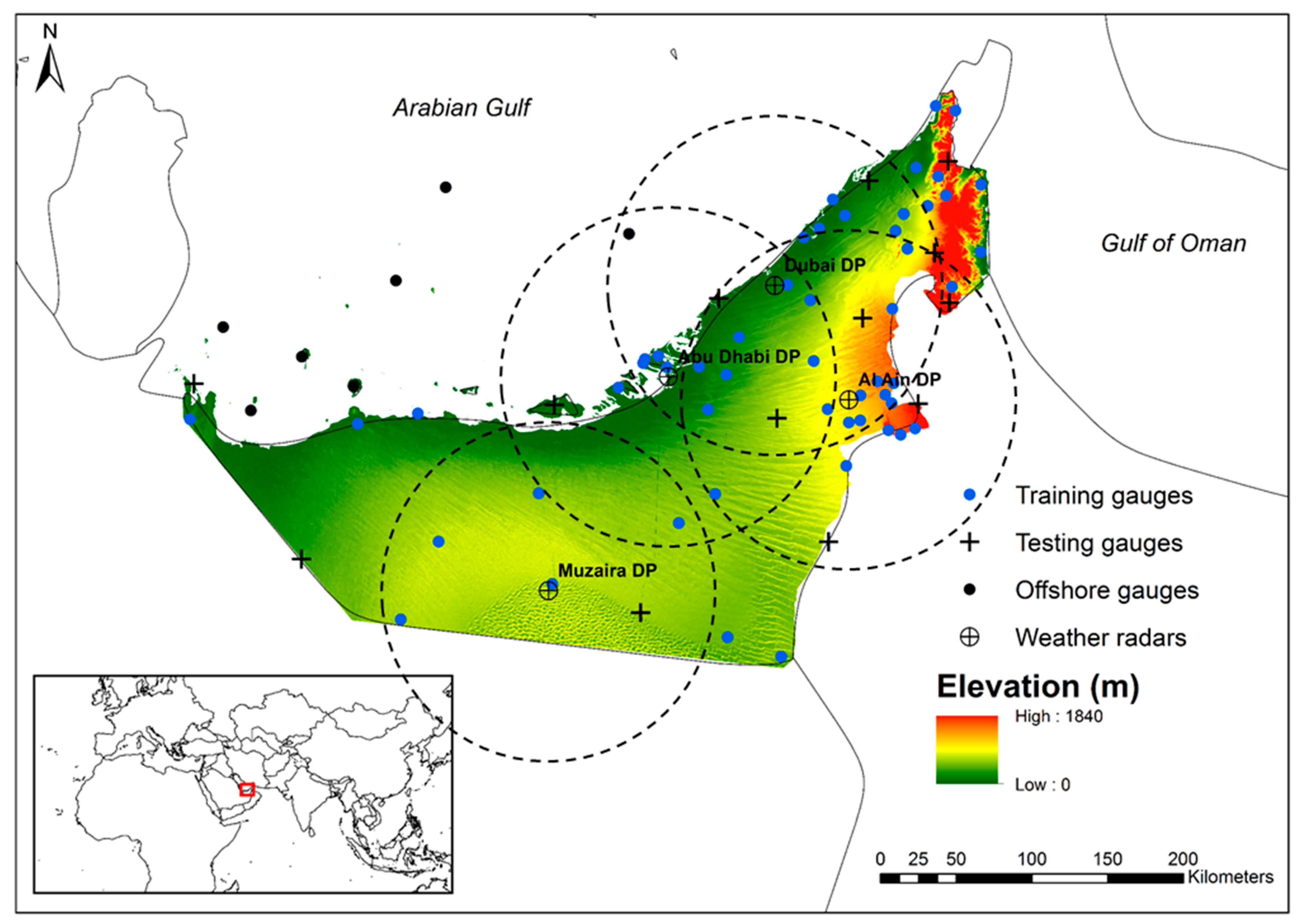
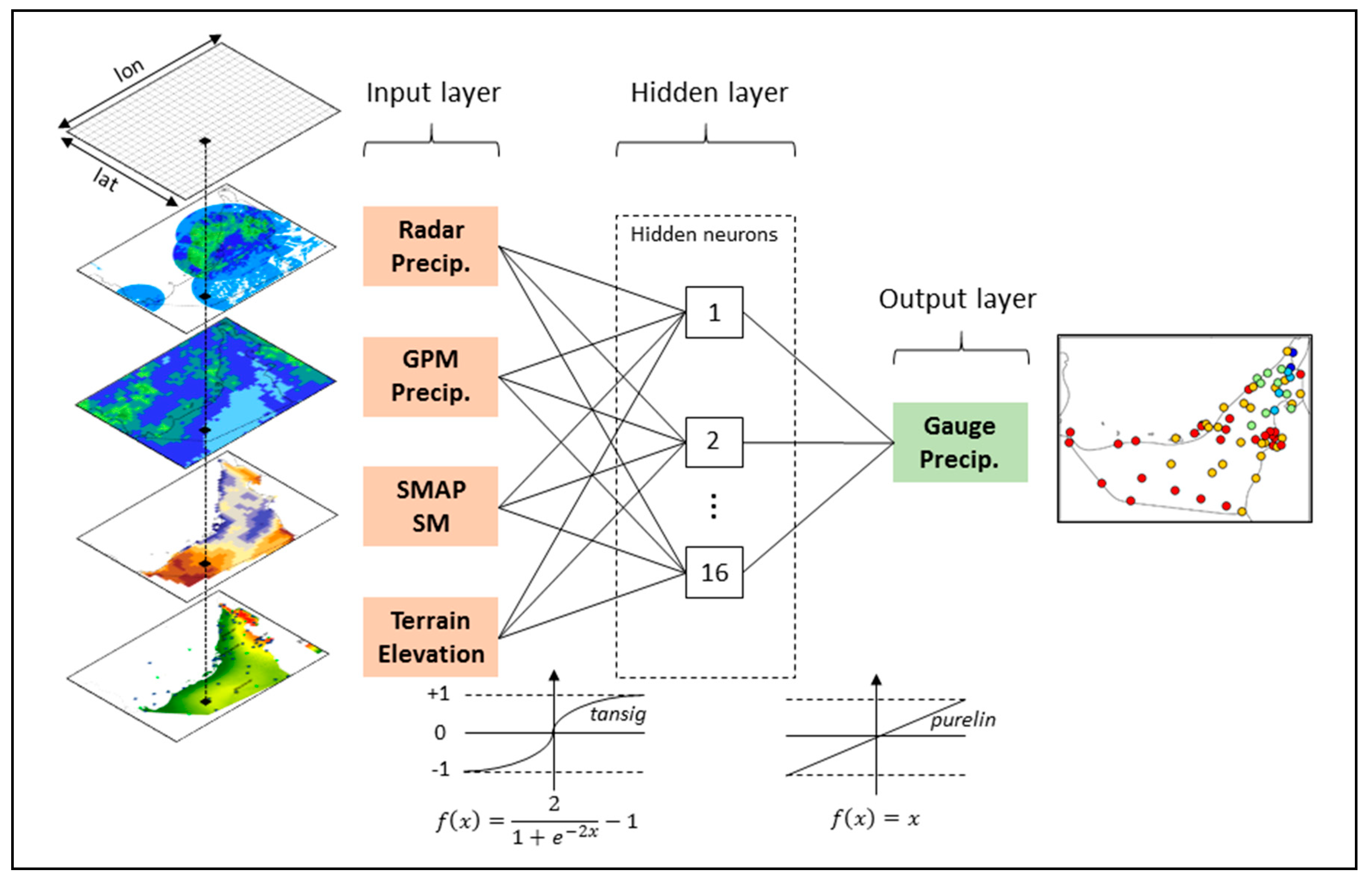
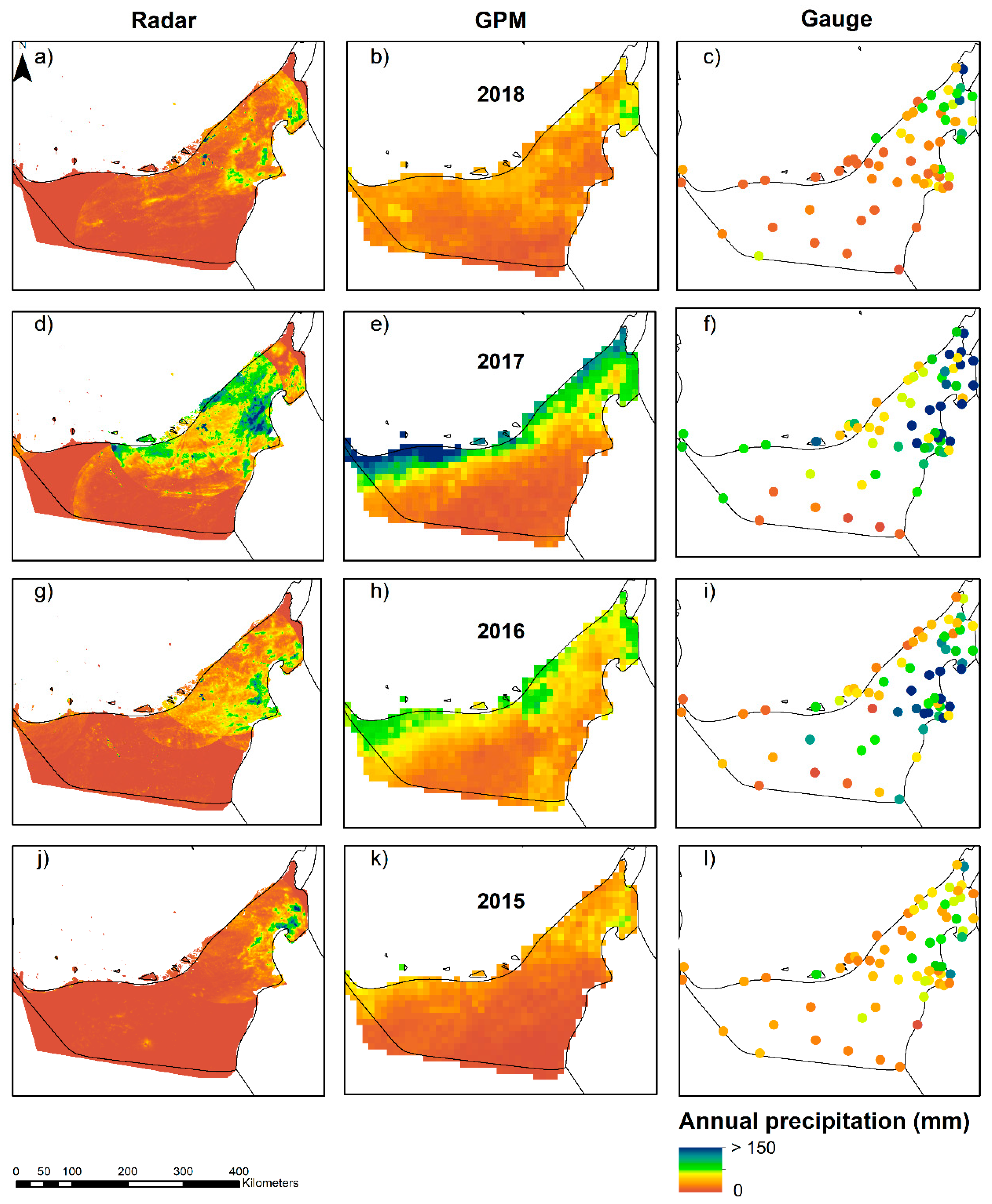
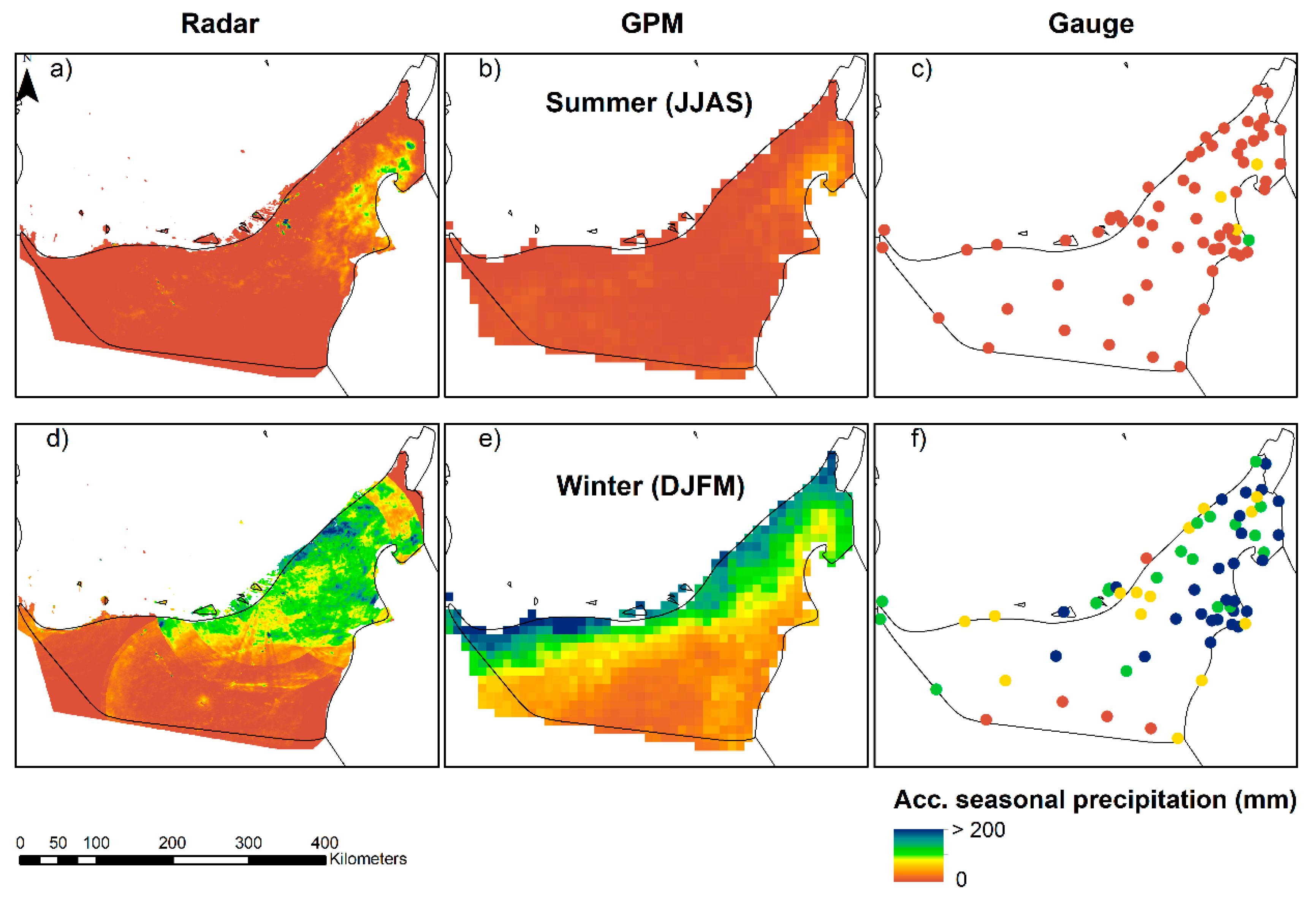
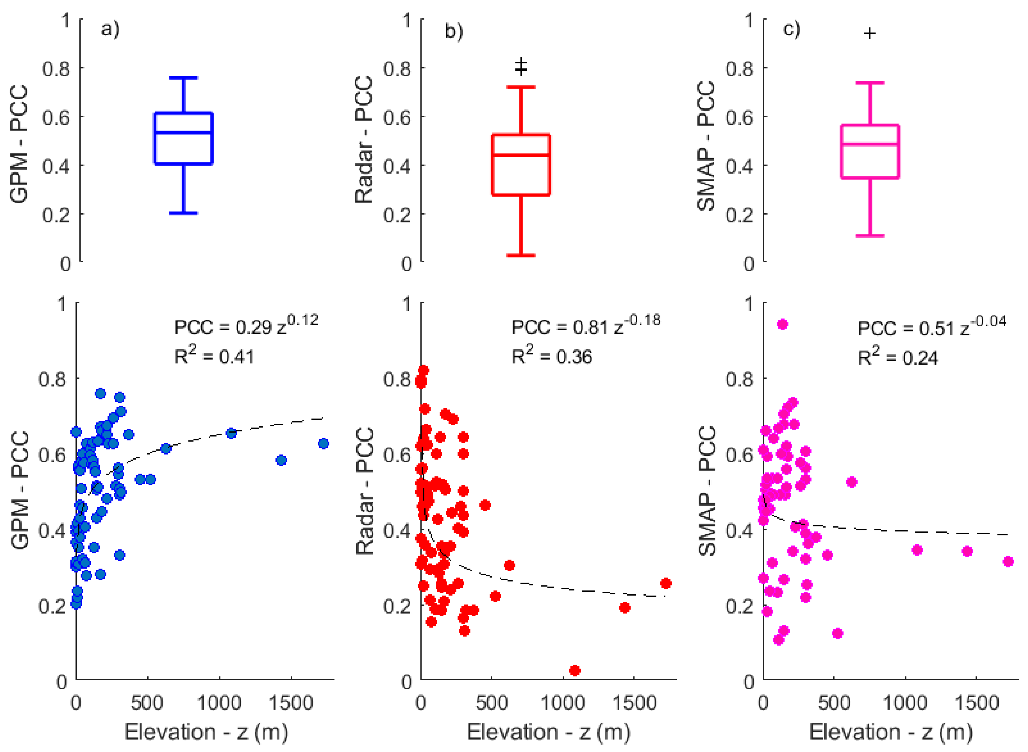
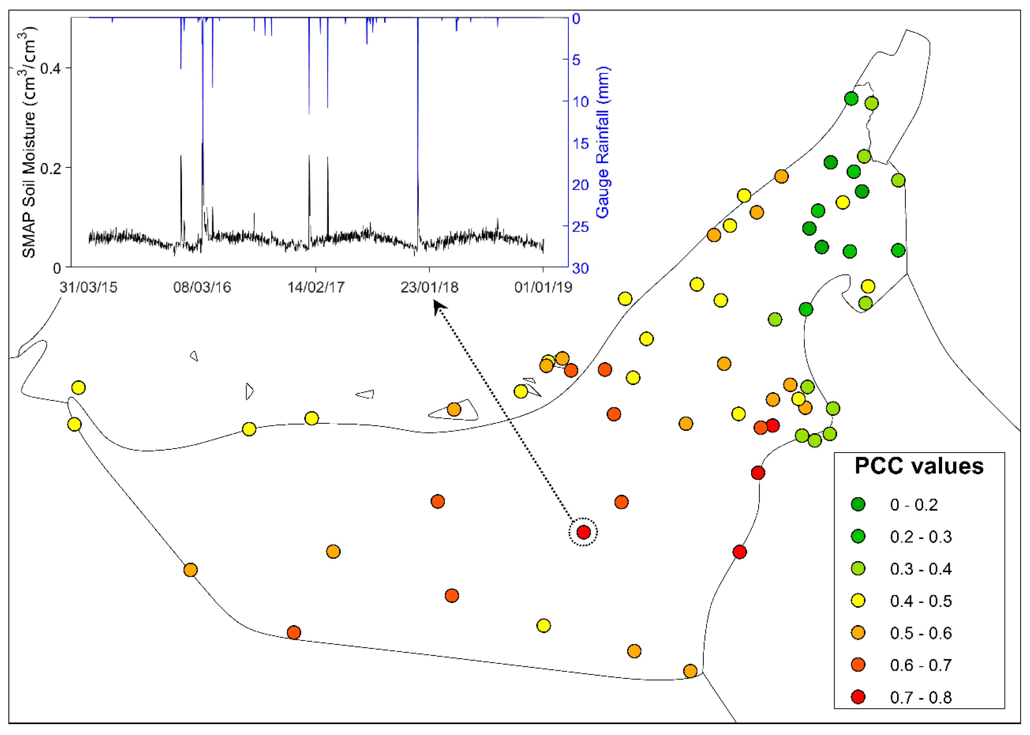
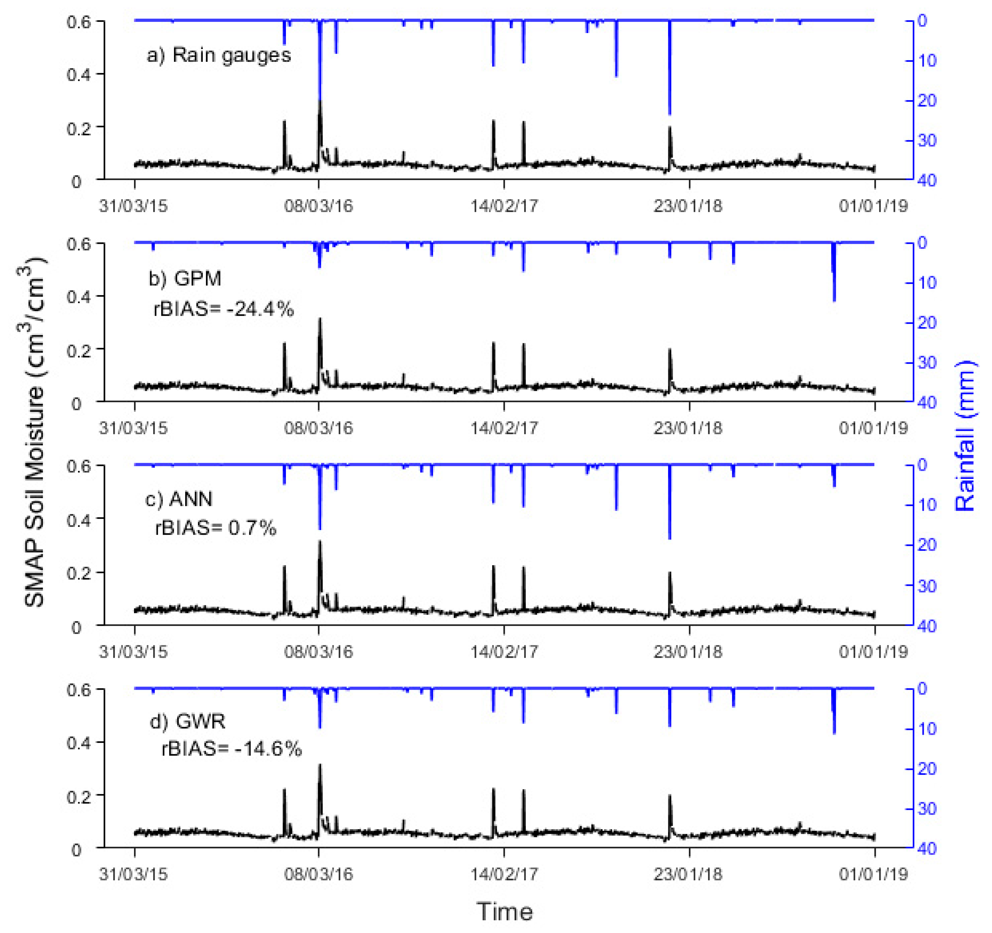
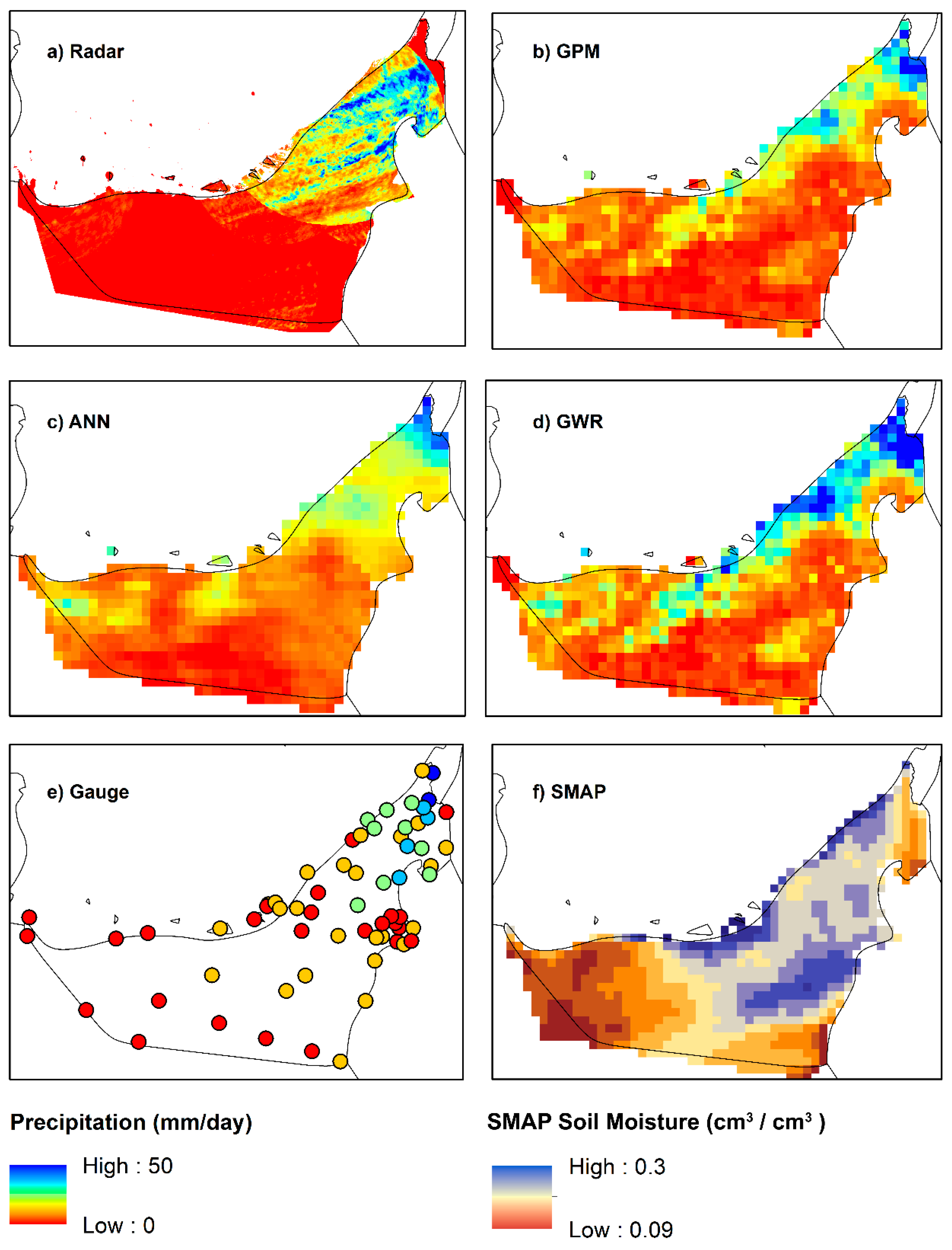
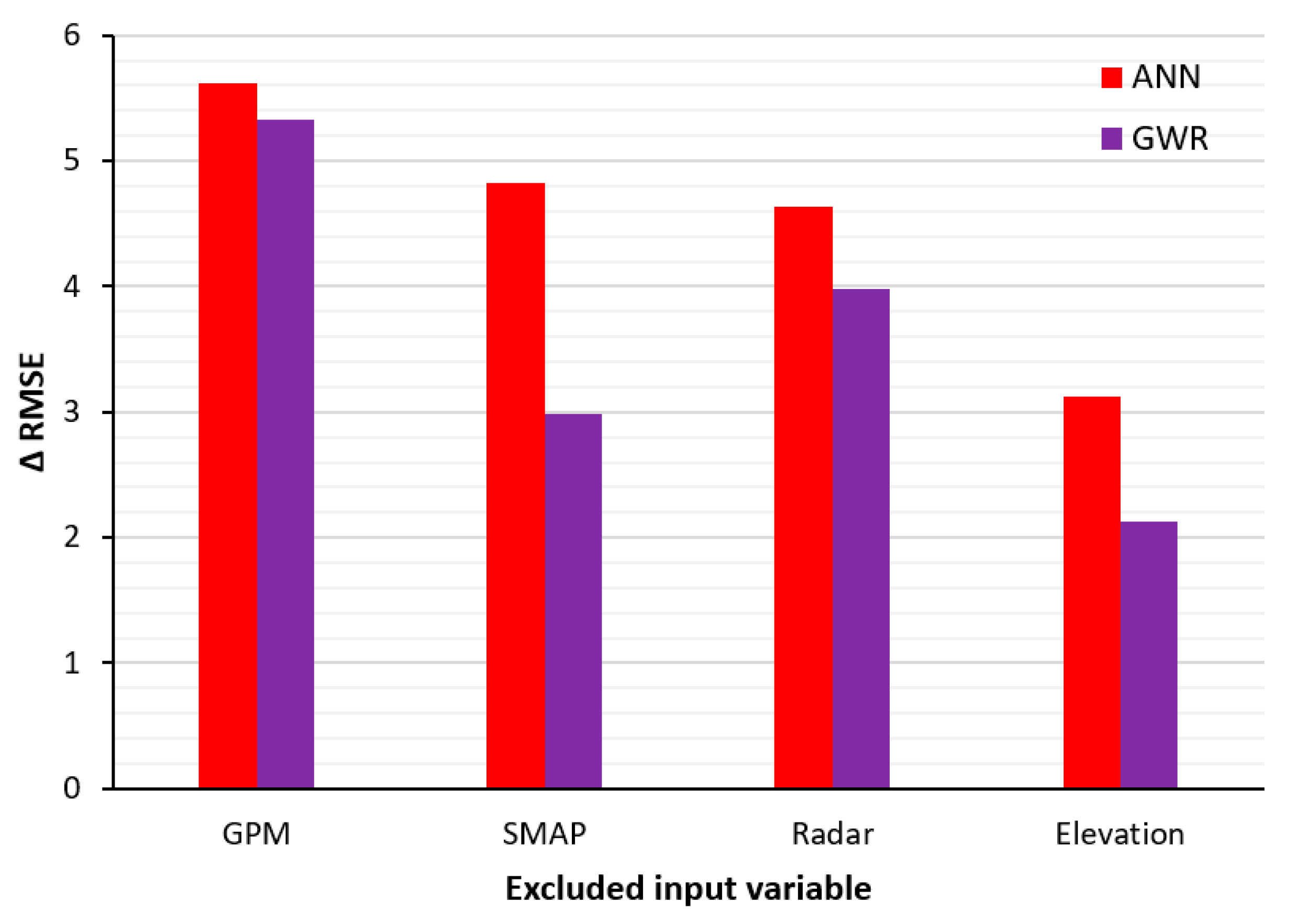
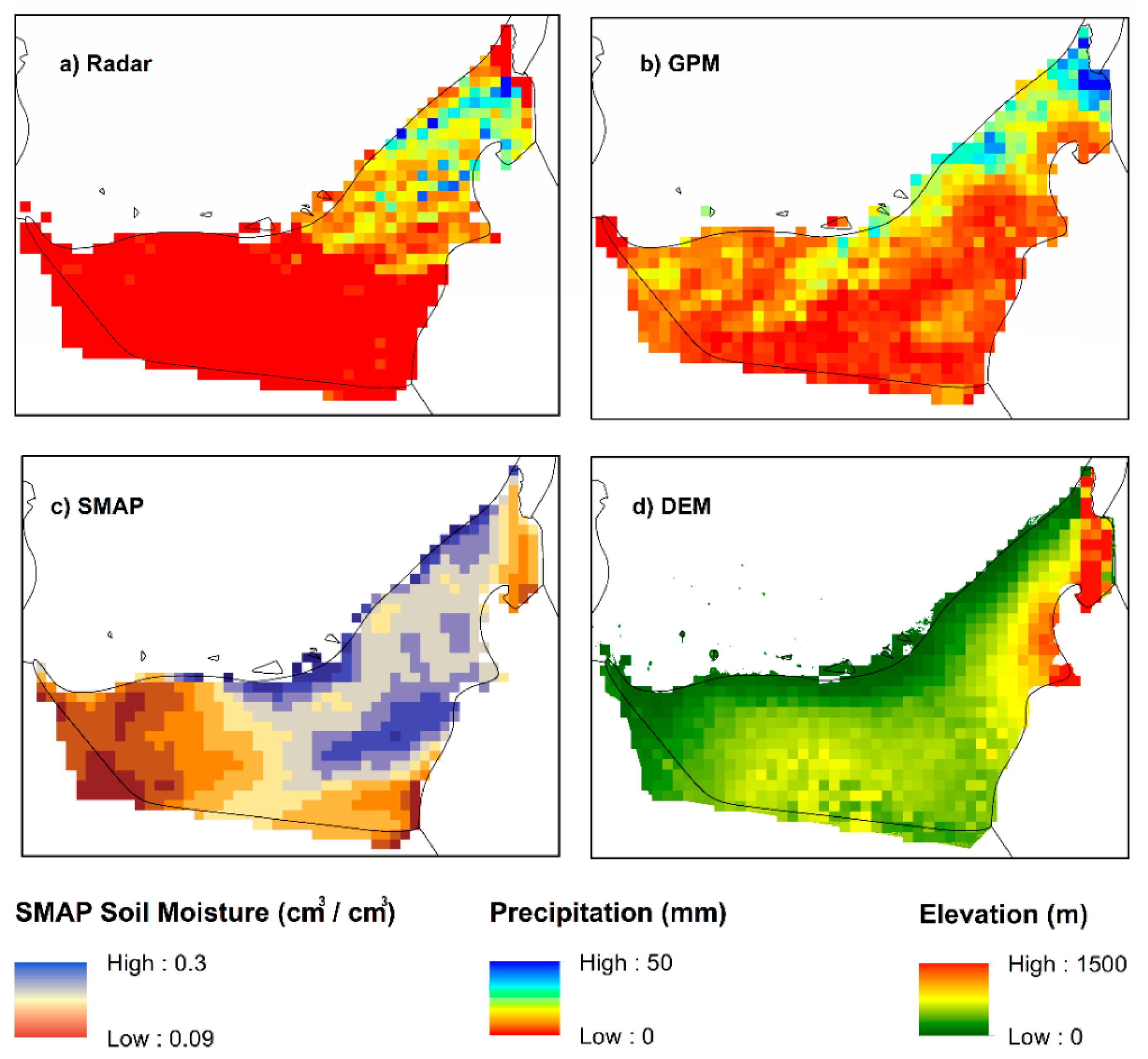
Table 1.
Overview of selected configuration and parameter values for the proposed ANN.
| Network Attribute | Value/Selection | Reasoning |
|---|---|---|
| No. of hidden layers | 1 | See [18,47,75] |
| No. of hidden neurons (n) | 16 | From 10-fold cross-validation [76] |
| Hidden and output layer activation functions | Hyperbolic tangent (tansig) and linear (purelin) transfers | See [18,77] |
| Training algorithm | Levenberg–Marquardt algorithm (trainlm) | See [18,71] |
Table 2.
Seasonal statistical error measures and skill scores recorded by the GPM, radar, GWR, and ANN estimates from SS (using the 13 testing gauges during the full period of 2015–2018) and TS (using all stations during 2018).
Table 2.
Seasonal statistical error measures and skill scores recorded by the GPM, radar, GWR, and ANN estimates from SS (using the 13 testing gauges during the full period of 2015–2018) and TS (using all stations during 2018).
| Source | rBIAS (%) | NSE | POD | FAR 1 | ||||
|---|---|---|---|---|---|---|---|---|
| Summer (JJAS) | ||||||||
| SS | TS | SS | TS | SS | TS | SS | TS | |
| GPM | −6.35 | −4.7 | 0.23 | 0.28 | 0.54 | 0.48 | 0.43 | 0.38 |
| Radar | 11.68 | 8.24 | 0.38 | 0.21 | 0.83 | 0.76 | 0.28 | 0.31 |
| GWR | −4.78 | −5.12 | 0.43 | 0.32 | 0.68 | 0.62 | 0.41 | 0.36 |
| ANN | 2.42 | 2.81 | 0.56 | 0.51 | 0.74 | 0.71 | 0.33 | 0.34 |
| Winter (DJFM) | ||||||||
| GPM | 18.42 | 14.21 | 0.41 | 0.29 | 0.72 | 0.61 | 0.36 | 0.43 |
| Radar | −9.12 | −11.13 | −0.19 | 0.11 | 0.68 | 0.58 | 0.41 | 0.48 |
| GWR | 7.84 | 10.42 | 0.44 | 0.38 | 0.76 | 0.67 | 0.33 | 0.39 |
| ANN | 5.43 | 6.89 | 0.54 | 0.48 | 0.81 | 0.73 | 0.27 | 0.35 |
1 3 mm threshold.
© 2020 by the authors. Licensee MDPI, Basel, Switzerland. This article is an open access article distributed under the terms and conditions of the Creative Commons Attribution (CC BY) license (http://creativecommons.org/licenses/by/4.0/).
Share and Cite
MDPI and ACS Style
Wehbe, Y.; Temimi, M.; Adler, R.F. Enhancing Precipitation Estimates Through the Fusion of Weather Radar, Satellite Retrievals, and Surface Parameters. Remote Sens. 2020, 12, 1342. https://0-doi-org.brum.beds.ac.uk/10.3390/rs12081342
AMA Style
Wehbe Y, Temimi M, Adler RF. Enhancing Precipitation Estimates Through the Fusion of Weather Radar, Satellite Retrievals, and Surface Parameters. Remote Sensing. 2020; 12(8):1342. https://0-doi-org.brum.beds.ac.uk/10.3390/rs12081342
Chicago/Turabian StyleWehbe, Youssef, Marouane Temimi, and Robert F. Adler. 2020. "Enhancing Precipitation Estimates Through the Fusion of Weather Radar, Satellite Retrievals, and Surface Parameters" Remote Sensing 12, no. 8: 1342. https://0-doi-org.brum.beds.ac.uk/10.3390/rs12081342
Note that from the first issue of 2016, this journal uses article numbers instead of page numbers. See further details here.