Coastal Wind Measurements Using a Single Scanning LiDAR
by
 , ,
, ,
Susumu Shimada
1,* ,
,
Jay Prakash Goit
1,2,
Teruo Ohsawa
3,
Tetsuya Kogaki
1 and
Satoshi Nakamura
4 1
Renewable Energy Research Center, National Institute of Advanced Industrial Science and Technology, Koriyama 963-0298, Japan
2
Department of Mechanical Engineering, Kindai University, Higashi-Hiroshima, Hiroshima 739-2116, Japan
3
Graduate School of Maritime Sciences, Kobe University, Kobe 658-0022, Japan
4
Coastal and Estuarin Environment Division, Port and Airport Research Institute, Yokosuka 239-0826, Japan
*
Author to whom correspondence should be addressed.
Remote Sens. 2020, 12(8), 1347; https://0-doi-org.brum.beds.ac.uk/10.3390/rs12081347
Submission received: 22 March 2020
/
Revised: 18 April 2020
/
Accepted: 21 April 2020
/
Published: 24 April 2020
(This article belongs to the Special Issue Assessment of Renewable Energy Resources with Remote Sensing)
Abstract
:A wind measurement campaign using a single scanning light detection and ranging (LiDAR) device was conducted at the Hazaki Oceanographical Research Station (HORS) on the Hazaki coast of Japan to evaluate the performance of the device for coastal wind measurements. The scanning LiDAR was deployed on the landward end of the HORS pier. We compared the wind speed and direction data recorded by the scanning LiDAR to the observations obtained from a vertical profiling LiDAR installed at the opposite end of the pier, 400 m from the scanning LiDAR. The best practice for offshore wind measurements using a single scanning LiDAR was evaluated by comparing results from a total of nine experiments using several different scanning settings. A two-parameter velocity volume processing (VVP) method was employed to retrieve the horizontal wind speed and direction from the radial wind speed. Our experiment showed that, at the current offshore site with a negligibly small vertical wind speed component, the accuracy of the scanning LiDAR wind speeds and directions was sensitive to the azimuth angle setting, but not to the elevation angle setting. In addition to the validations for the 10-minute mean wind speeds and directions, the application of LiDARs for the measurement of the turbulence intensity (TI) was also discussed by comparing the results with observations obtained from a sonic anemometer, mounted at the seaward end of the HORS pier, 400 m from the scanning LiDAR. The standard deviation obtained from the scanning LiDAR measurement showed a greater fluctuation than that obtained from the sonic anemometer measurement. However, the difference between the scanning LiDAR and sonic measurements appeared to be within an acceptable range for the wind turbine design. We discuss the variations in data availability and accuracy based on an analysis of the carrier-to-noise ratio (CNR) distribution and the goodness of fit for curve fitting via the VVP method.
1. Introduction
The global offshore wind energy market has been continuously growing with 4.5 GW of new wind turbines installed in the year of 2018, bringing the total cumulative installations to 23 GW [1]. Although offshore wind energy, which currently represents a global share of four percent of the total cumulative wind power generation, is significantly smaller compared to the onshore wind market, offshore wind has huge potential and is poised to grow with a stable addition from Europe and significant contributions from the emerging markets of Asia. According to the Global Wind Energy Council (GWEC), the annual offshore installations is expected to exceed 6 GW in the near future [1]. For instance, the interest in offshore wind installations in Japan was stimulated by the recently announced maritime renewable energy policy of the Japanese government [2]. However, offshore wind energy poses several challenges right from the early phase of development. One of the foremost challenges faced by the developer is the accurate and economic means of wind resource assessment at the prospective offshore wind farm sites. Unlike onshore sites, where a meteorological mast (met mast) can be constructed with relative ease, building offshore met masts for the same purpose can involve serious technical and financial challenges. As an alternative to met masts, wind resource assessment using light detection and ranging (LiDAR) has received significant interest in the wind energy community [3,4,5,6,7]. The current work aims to investigate the performance of a scanning Doppler LiDAR for wind resource assessment in the nearshore region, which is considered promising for the development of fixed-bottom offshore wind farms.
In several emerging markets, including Japan, most offshore wind farms are likely to be constructed just a few kilometers off the coast, because the water depth increases rapidly further offshore and the development becomes more costly. Therefore, accurate characterization of the coastal wind is crucial. In this regard, Shimada et al. [7] conducted measurements using two profiling LiDARs at the landward and seaward ends near the coast and found that the wind speeds could increase by up to 120% at a distance of 2 km off the coast. They also showed that the differences between the onshore and offshore winds were less pronounced at higher altitudes. In the follow-up study, they performed mesoscale simulations assimilating profiling LiDAR observations from the coast to reduce the uncertainty in nearshore wind resource predictions [8].
Contrary to the vertical profiling LiDARs, scanning Doppler LiDARs can accommodate measurement ranges from 3 to 10 km [9]. Therefore, they offer the potential for assessing offshore wind from the coast, thus obviating the need for offshore met masts or floating LiDARs [10,11,12]. To date, scanning LiDARs have been used for the measurements of wind fields and, most importantly, turbulence in single or multi-LiDAR modes [13,14,15,16]. Scanning LiDARs have also been used in the measurements of flow fields around a wind turbine or to evaluate wind turbine power performance [17,18]. However, these studies and other similar works in the literature mainly conducted short-term measurement campaigns, while actual wind resource assessment requires long-term wind statistics, e.g., mean wind speeds over a period of a few months to one year.
Several projects on the application of scanning LiDARs for wind resource assessment are introduced here [19,20,21,22]. Cameron et al. [19] reported validation results using a dual scanning LiDAR system in Dublin Bay. Two scanning LiDARs used in the study were at distances of 15.9 and 8.8 km from the validation target. Courtney et al. [20] and Simon and Courtney [22] conducted validation campaigns at a test site at the Danish Technical University, testing several scanning patterns from a point 1.5 km from the target met mast. The results indicate that a scanning configuration with an azimuth width of 45° and a scan rate of 3°/s showed the best performance. Coutts et al. [21] also showed validation results with a distance of approximately 1.8 km at a German test site. Some of the reports have shown good agreement with observations obtained from met masts. However, details of the validation methods employed, such as the horizontal wind retrieving algorithm used in the analysis, have not been made available. Thus, the usefulness of a scanning LiDAR for wind resource assessment over coastal waters has remained ambiguous.
In the current study, we conducted an offshore wind measurement campaign with a single scanning Doppler LiDAR installed at a coast in central Japan. The horizontal wind speeds and wind directions were retrieved from the LiDAR-measured radial wind speeds using the velocity volume processing method. One of the objectives of this study was to investigate the effect of the scan parameters, such as the azimuth range and elevation angle on the quality of measured wind speeds. Furthermore, the effects of the wind direction and data availability on the accuracy of the retrieved wind speeds is also analyzed. The ability of a scanning LiDAR to measure the turbulence intensity (TI) was also investigated. To that end, scanning LiDAR measurements were compared against the data from a profiling LiDAR and a sonic anemometer at the site.
The paper is organized as follows. In Section 2, we describe the measurement site and devices. The measurement cases and velocity retrieval techniques are also presented in this section. In Section 3 and Section 4, we present our results and related discussions. The main conclusions of this work are summarized in Section 5.
2. Materials and Methods
2.1. Experimental Setup
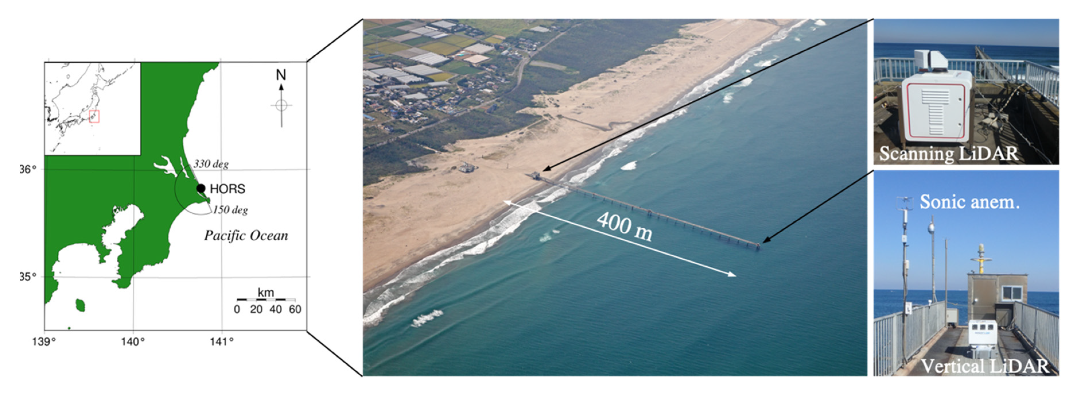
The measurement campaign was conducted from January to September 2019 at the Hazaki Oceanographic Research Station (HORS) [23]. The HORS is located at the coastline of the Pacific Ocean in Ibaraki prefecture, Japan. This region has a rectilinear coastline running from 150° to 330° and is surrounded by flat terrain with mixed vegetation. Figure 1 shows the instruments used in the study and the positions on the HORS pier where they were placed. The pier is 427 m long and at a height of 7 m above sea level (ASL). As 1.5 MW wind turbines with a hub height of 64.5 m and a rotor diameter of 62 m align along the coast, the winds on the pier at a wind direction of approximately 207° are directly influenced by the wind turbine wake. Detailed wind conditions on the HORS research platform can be found in Shimada et al. (2018) [7].
Table 1 summarizes the list of the measurement devices used in this study. The scanning LiDAR (Windcube 100s, hereafter referred to as the 100s) was deployed on the roof of a 3.5-m-high observational facility located at the landward end of the HORS pier. The dimensions of the scanning LiDAR were approximately 0.8 m × 1.0 m × 1.2 m and it weighed 235 kg. This LiDAR had a measurement range from 50 to 3000 m, with a horizontal resolution, which can be set between 25 and 100 m. Further specifications of the 100s are available on the manufacturer’s website [9]. For validation of the wind speeds and directions obtained from the 100s, the offshore measurements from a sonic anemometer (hereafter referred to as SA) and a vertical profiling LiDAR (Windcube V1, hereafter referred to as V1) installed at the seaside end of the pier were used. The measurements from the V1 were mainly used for the validation of the 10-minute mean wind speeds, while those from the sonic anemometer (SA) were used to assess the accuracy of the turbulence intensity (TI) measurements.
2.2. Leveling Calibration of the Scannig LiDAR
It is best to have the scanning LiDAR installed in a perfectly level position, as a tilted device results in differences between the target and the actual measurement points. In particular, a tilt angle in the vertical direction can significantly affect the accuracy of wind speed measurements taken with a scanning LiDAR due to the strong vertical wind shear that exists within the surface layer. The impact of a tilt angle increases linearly with the distance from the device. For instance, a device deployed with a tilt angle of 1° leads to vertical height errors of 17.5 and 35 m, respectively, at the ranges of 1000 and 2000 m. This will consequently introduce extra uncertainty into the wind speed measurements.
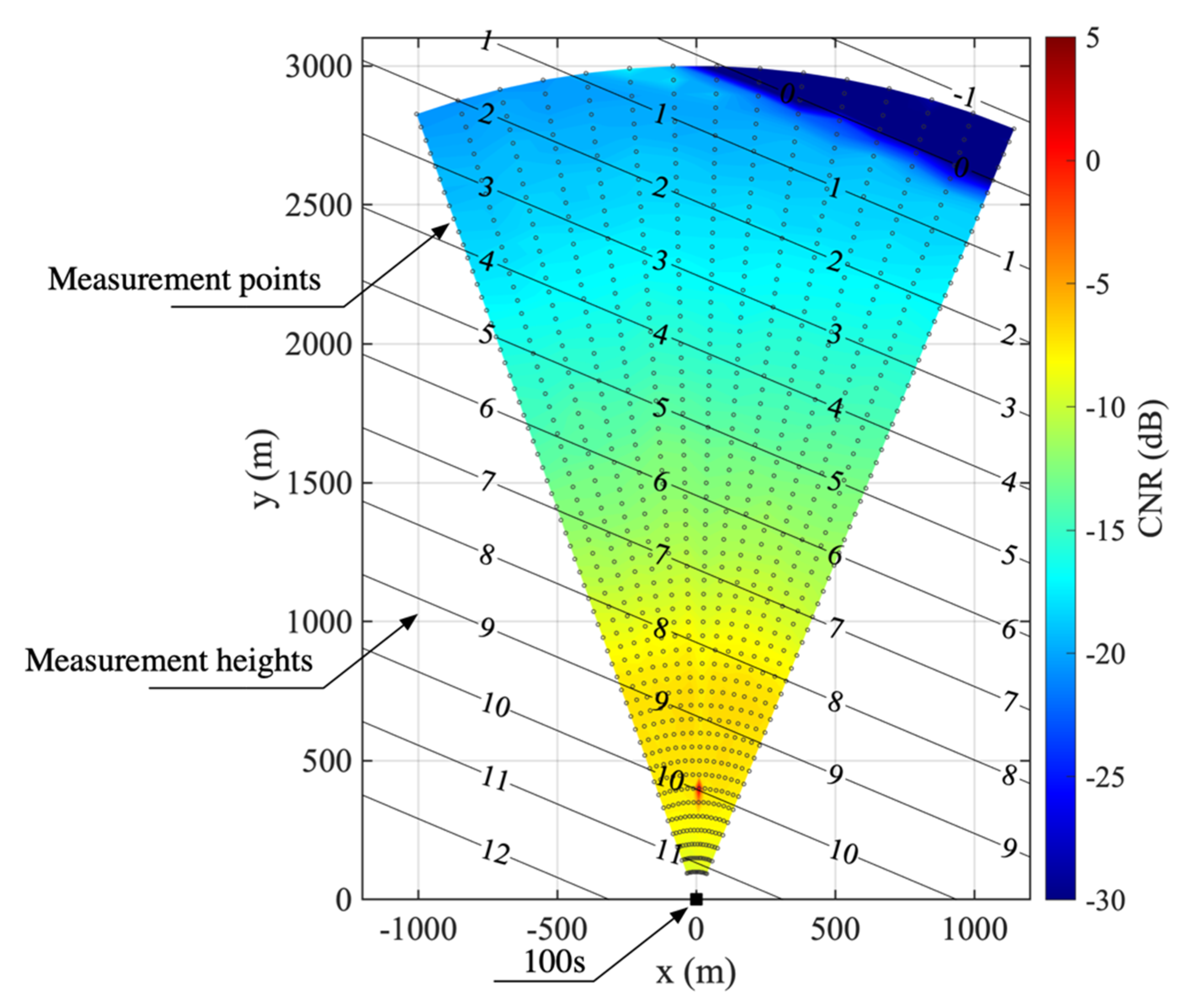
Field measurement environments differ from laboratory environments, and it appears difficult to deploy a scanning LiDAR with a tilt angle error of less than 0.1° (the impact of which can be assumed to be negligibly small), even using extremely precise digital levels. Therefore, a calibration method referred to as hard target calibration (HTC) [19] was used for the leveling calibration. In HTC, the tilt angle is generally estimated by analyzing the carrier-to-noise ratio (CNR) values, which are used for checking the quality of measurements. Generally, the CNR values peak near the device, then decrease as the distance increases. Moreover, it is also known that scanning LiDARs record dramatically higher CNR values when the laser is reflected by obstacles such as a meteorological tower or light house.
By using characteristics of the CNR recorded by scanning LiDARs when striking an obstacle, the pitch and roll angles of the device, which are the tilt angles in the x and y directions, respectively, can be estimated from the difference between the actual location of the obstacle and the position detected by the CNR distribution of the scanning LiDAR. After calculating the pitch and roll angles, they are added to the original LiDAR-registered azimuth and elevation angles as an offset. This approach, using the reflection from obstacles, is applicable with fewer constraints over land, but is difficult to apply to offshore wind measurements due to the difficulty of finding suitable targets offshore.
Therefore, in the current study, another characteristic of the CNR distribution of the LiDAR was used to estimate the pitch and roll angles misalignment. At the time of installation, we noticed that the CNR appeared to rapidly decline when the laser beam hit the sea surface. Figure 2 shows a snapshot of the CNR distribution obtained from the 100s with an azimuth width of 45° and for an elevation angle of 0°. The Japanese Local Standard Time (LST), which is +9 hours from UTC, is used in this study. The high CNR values at the x and y positions of 0 and 400 m were due to the reflection from the observational hut on the pier. Much lower CNR values are observed in the upper right region of the figure. As an elevation angle of 0° was set in this case and no obstacle was present, this must be the result of the laser beam hitting the water surface in this region. From this CNR distribution, we were able to estimate the pitch and roll error using planar fitting, as the horizontal and vertical positions of the LiDAR device are the given information. The equation of the planar fitting is given by
where is the deployment height of the 100s (= 11.5 m ASL), and and are the pitch and roll angles. For the LiDAR installation in the current study, a pitch angle of −0.092° and a roll angle of −0.217° were obtained by applying this method. In Figure 2, the contour of the measurement heights, taking into account the pitch and roll angles derived from the planar equation, is overlaid. The pitch and roll angles estimated here were used when calculating the height at each measurement point from the azimuth and elevation angles in the wind speed retrieval process. In contrast to the HTC approach, we call this approach soft target calibration (STC).
2.3. Scanning Mode and the Velocity Volume Processing (VVP) Method
2.3.1. Scanning Mode
Four scanning modes were available for the 100s: the plan position indicator (PPI) mode, range height indicator (RHI) mode; Doppler beam swinging (DBS) mode, and fixed mode. The choice of scanning mode depends on the purpose of the measurements. The RHI mode and the fixed mode are frequently used for wind turbine wake measurements [15,16] and virtual met tower measurements [24], respectively. The current study uses the PPI mode, as it is compatible with the VVP method [25,26,27] for retrieving horizontal wind speeds and directions from the LiDAR-measured radial wind speeds.
In the PPI mode, the scanning LiDAR measures the radial wind speeds by sweeping the scanning head over a range of azimuth angles while the elevation angle is fixed. In this study, a scanning range of up to 3000 m, with a radial resolution of 50 m and a data accumulation time of 1 s, were employed as the scan settings. The data accumulation time is the integration interval used to derive each radial wind speed. As the azimuth and elevation angle settings, such as the scanning width and scan rate, would be the primary factors affecting the accuracy of the wind speed measurements, the PPI measurements were carried out using different azimuth and elevation angles in this study.
Table 2 lists the experimental duration and scan settings for each experimental case. The reference sensor (V1 or SA) used for each validation is shown in the column. The evaluation height for each case is also described in the table. The impacts of the azimuth angle settings were investigated in the experiments for Cases 1 through 5. In Cases 1 to 4, the accuracies of the wind speeds at a height of 47 m were compared for four different azimuth widths. In Case 5, the settings were identical to those in Case 4 except for the scan rate, which was reduced to 1° (from 3°) so that the number of data at the given radial position increased. This allowed us to investigate the effect of the number of input data on the quality of wind speed computed using the VVP method. In Case 6 and Case 7, the impact of the elevation angle on the measurement accuracy was investigated by comparing the results for different elevation angles. Case 8 had identical settings to those of Case 2, but ran for a longer period, to assess the impact of the wind direction. In addition to the validation of the 10-minute mean wind speeds and wind directions, the accuracy of the TI values was also examined by comparing them against the measurements obtained from the SA in Case 9.
2.3.2. Velocity Volume Processing (VVP)
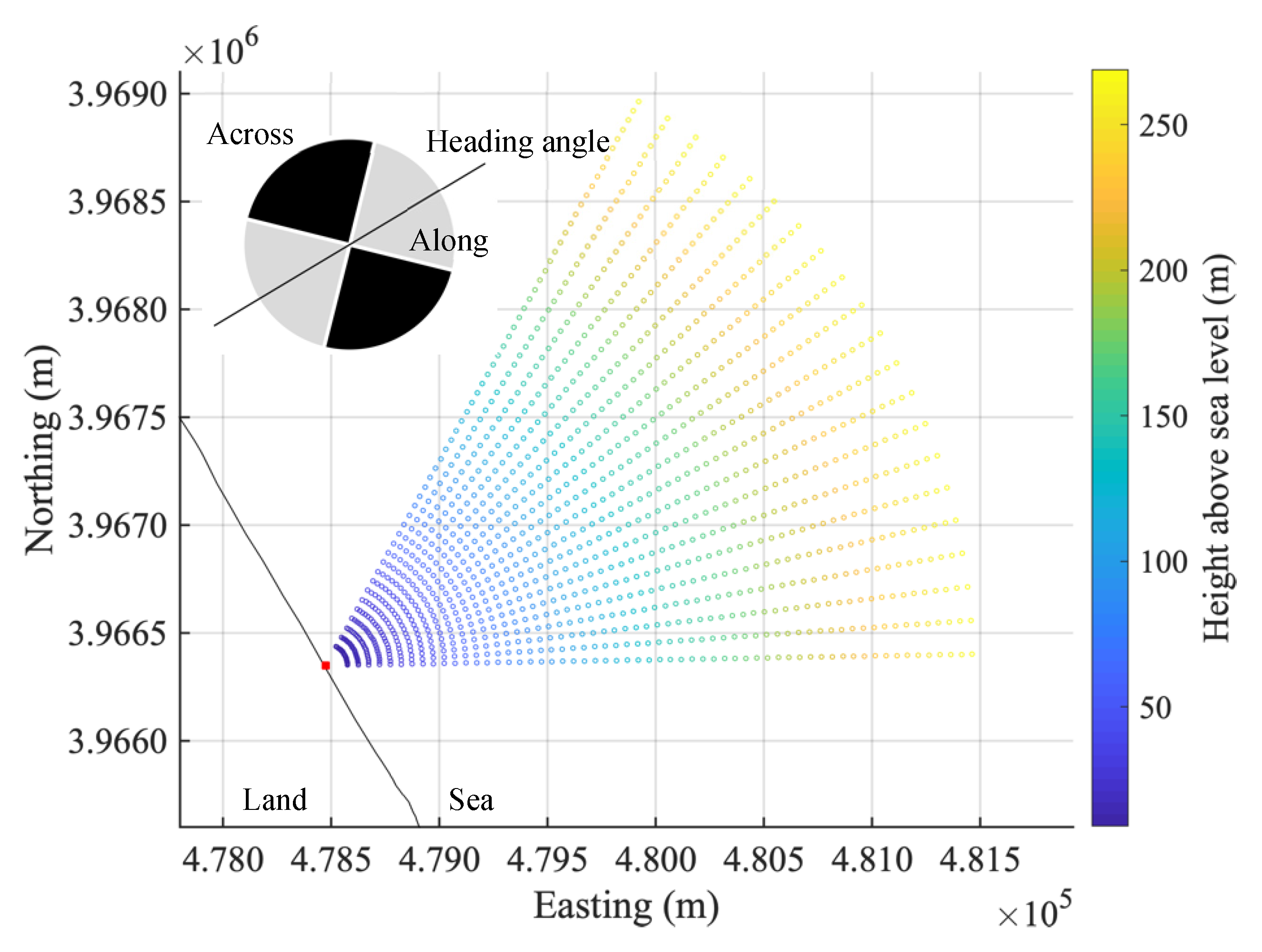
Figure 3 illustrates the schematic of the measurement positions and heights for Case 1. The small red square and the diagonal line passing through indicate the 100s and the coastline, respectively. The heading angle of the 100s and the along- and across-wind direction sectors are shown in the pie chart in the upper left corner. The radial wind speeds were measured along the line of the colored dots, with the measurement line moving to the next position at an interval of 1 s. For this case (i.e., Case 1), it takes roughly 20 s to complete a cycle; the device then repeats the operation. A set of radial wind speeds for an arc at the same radial distance was used to compute the horizontal wind speeds and directions in the process of wind vector retrieval using the VVP method.
As noted earlier, the radial wind speeds obtained from the 100s were converted to horizontal wind speeds using the VVP method, which is discussed next. The radial wind speed can be expressed as the projection of the actual velocity vector along the radial direction, i.e.,
where is the radial wind speed, , , and are the horizontal and vertical wind speed components, is the elevation angle, and is the azimuth angle. In the original VVP, the wind speed is assumed to vary linearly about the analysis point, thus resulting in derivative terms of each wind speed component along all three spatial directions [26,27]. Therefore, in total, there will be 12 parameters on the right-hand side of Equation (2). As it is unnecessary to have the full set of these parameters for wind resource assessment considered in this study, we used an assumption to simplify the equation, following previous studies [25]. If we assume that the wind field is homogeneous in time and space for one scan cycle, and that the vertical component is negligibly small compared to the horizontal wind speed components, Equation (2) can be written as
As , , and are obtained from the 100s, and can be simply computed using the linear-least-squares method. The equation used in the least square method can be expressed as the following cost functional, which can be minimized for and :
where N is the number of scans during a sweep and Vr’ = Vr/cosθ. The condition for the minimization the cost functional is that its gradient with respect to the velocity is 0, i.e.,
This leads to the following equation that is solved in this study:
We tested other more sophisticated numerical approaches for solving Equation (3), such as a non-linear fitting method; however, the results are not significantly different for the above discussed approach. This can be attributed to the simplicity of the equation.
Before retrieving the horizontal wind speeds and directions using the VVP method, some pre-processing of the raw radial wind speed data was necessary. The raw measurements recorded by the V1 included not only instantaneous radial wind speeds but also a confidence index indicating the reliability of the various measurements diagnosed by the hardware. To screen out unreliable data, observations without a confidence flag were excluded from the analysis. As a pre-processing step for the curve fitting, a linear interpolation in the vertical direction was applied to the radial wind speed to adjust for the measurement height difference between the reference sensor (V1 or SA) and the 100s. The pitch and roll angle offsets described in Section 2.2 were also taken into account during this vertical interpolation procedure.
Following this vertical interpolation, we applied noise reduction to the measured radial wind speed. The measurement uncertainty of the scanning LiDARs was higher than that of the vertical profiling LiDARs. According to the device specifications, the 100s has a measurement uncertainty of 0.5 m/s for radial wind speed, while most vertical profiling LiDARs have an uncertainty of less than 0.2 m/s for horizontal wind speed. To reduce the noise in the raw data, a first-order low-pass filter with a recursive expression was applied. This is given by
where indicates the filtered radial wind speed at the previous time step and (= 0.3) is a smoothing factor. This process is useful for eliminating spikes in the data time-series.
In the analysis code, the values of and were calculated by solving Equation (6) using the radial wind speeds for a sweep, i.e., one cycle in the PPI scan. Thus, the temporal resolution of the wind speed obtained from the 100s depended on the azimuth width and scan rate. For example, the wind speeds and directions for Case 1 ( = 60°, = 3°/s) had a temporal resolution of approximately 20 s. From the instantaneous wind speeds and directions with an interval of 20 s, we calculated the 10-minute means and standard deviations. These were then compared to the reference observations from V1 or SA. As the data availability of the LiDARs depends on the atmospheric conditions, if the availability during the 10-minute interval was less than 80%, the measurements were excluded from the validation.
3. Results
3.1. Wind Condition during the Experimental Campaign
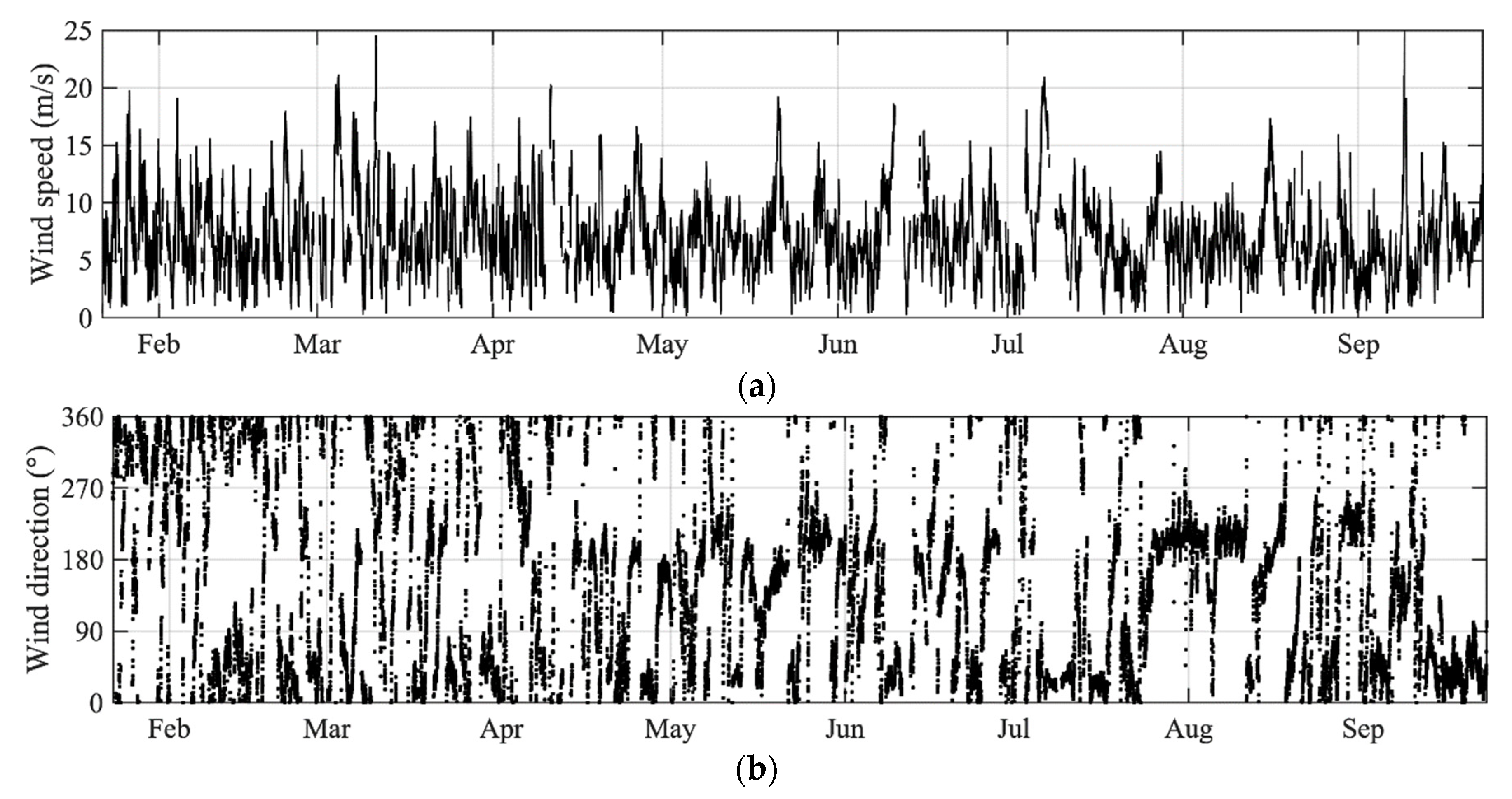
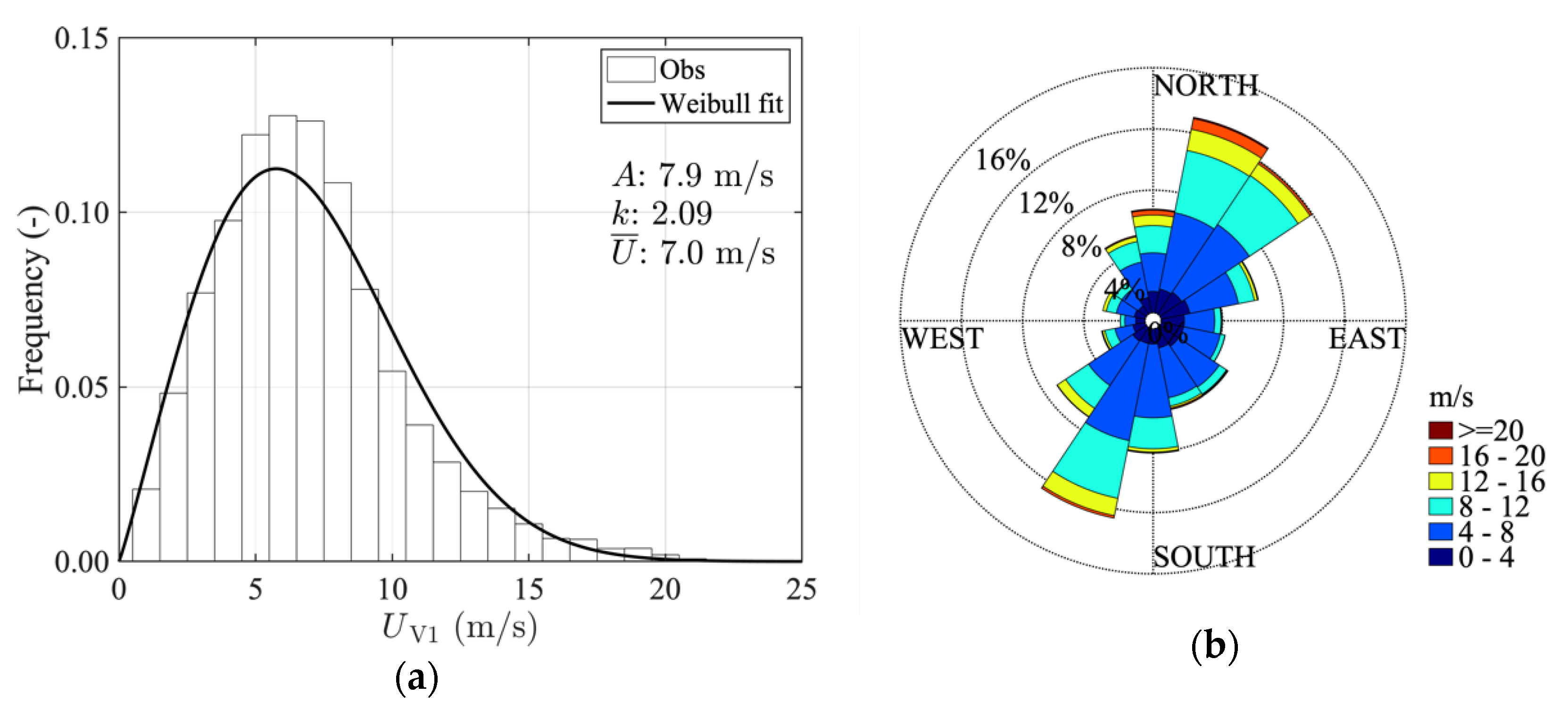
Before presenting the VVP-processed results, we briefly describe the wind characteristics of the measurement site. Figure 4 shows the time series of wind speeds and wind directions at a height of 107 m ASL obtained from V1 during the current measurement period (22 January to 23 September 2019). The data availability for V1 during this period was 91%. Figure 5 presents the distribution of these wind speeds and wind directions in the form of occurrence frequencies and a wind rose. Figure 5a also presents the Weibull probability density function (PDF) obtained by fitting to the following Weibull function:
where indicates the horizontal wind speed, is the shape parameter and is the scale parameter. For the current site, and . Furthermore, a mean wind speed of 7.0 m/s was observed. A north-easterly wind was dominant during the experimental period, though a south-westerly wind was also significant. A typhoon approached HORS on 8 to 9 September 2019, when strong winds with more than a 35 m/s 10-minute mean were observed.
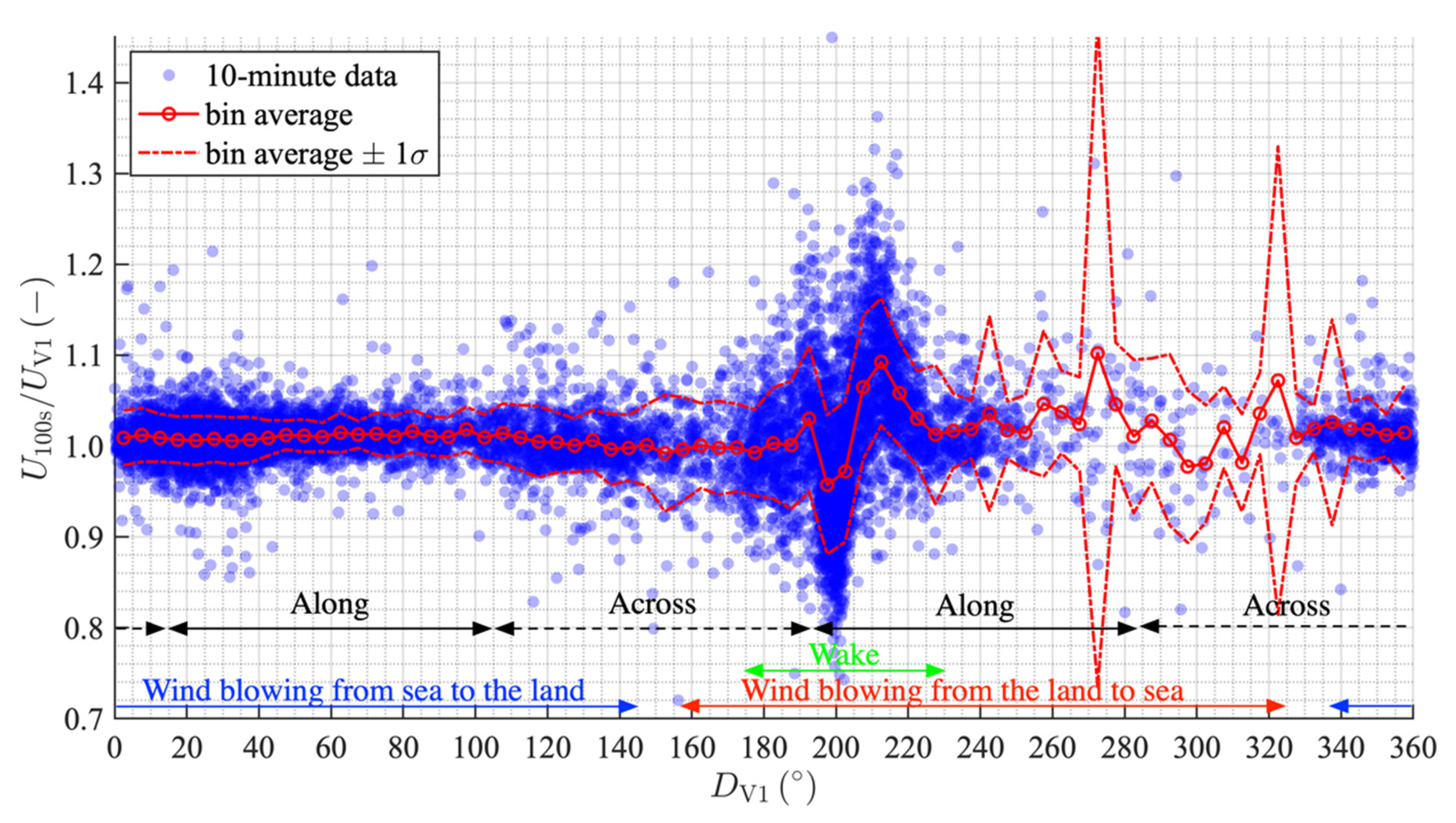
As described in Shimada et al. (2018) [7], at the HORS site, winds coming from 335° to 145° were categorized as sea winds (from sea to land sectors), while those from 155° to 325° were categorized as land winds (from land to sea sectors). Notably, land winds coming from between 175° and 230° were influenced by the neighboring wind turbines situated on the coastline. As a homogeneous wind field was assumed in the VVP method, the winds blowing from the wake sector may reduce the measurement accuracies, relative to the other sectors. Consequently, observations with a wind direction that was directly disturbed by the wake of the wind turbines were excluded from the validation.
3.2. Validation of 10-Minute Mean Wind Speeds and Wind Directions
3.2.1. Sensitivity to the Azimuth Angle Settings
Following the validation approaches recommended in previous studies [10,28,29], the accuracy of the offshore wind measurements using a single scanning LiDAR and the VVP method was quantitatively evaluated. The observations recorded during low wind conditions, when the V1 wind speeds were less than 2 m/s, were excluded from the analysis. Finally, as the measurements of V1 for wind directions around 207° were directly influenced by the wind turbines situated on the coast, the observations with a wind direction range of 207° ± 10° were also excluded from the analysis.
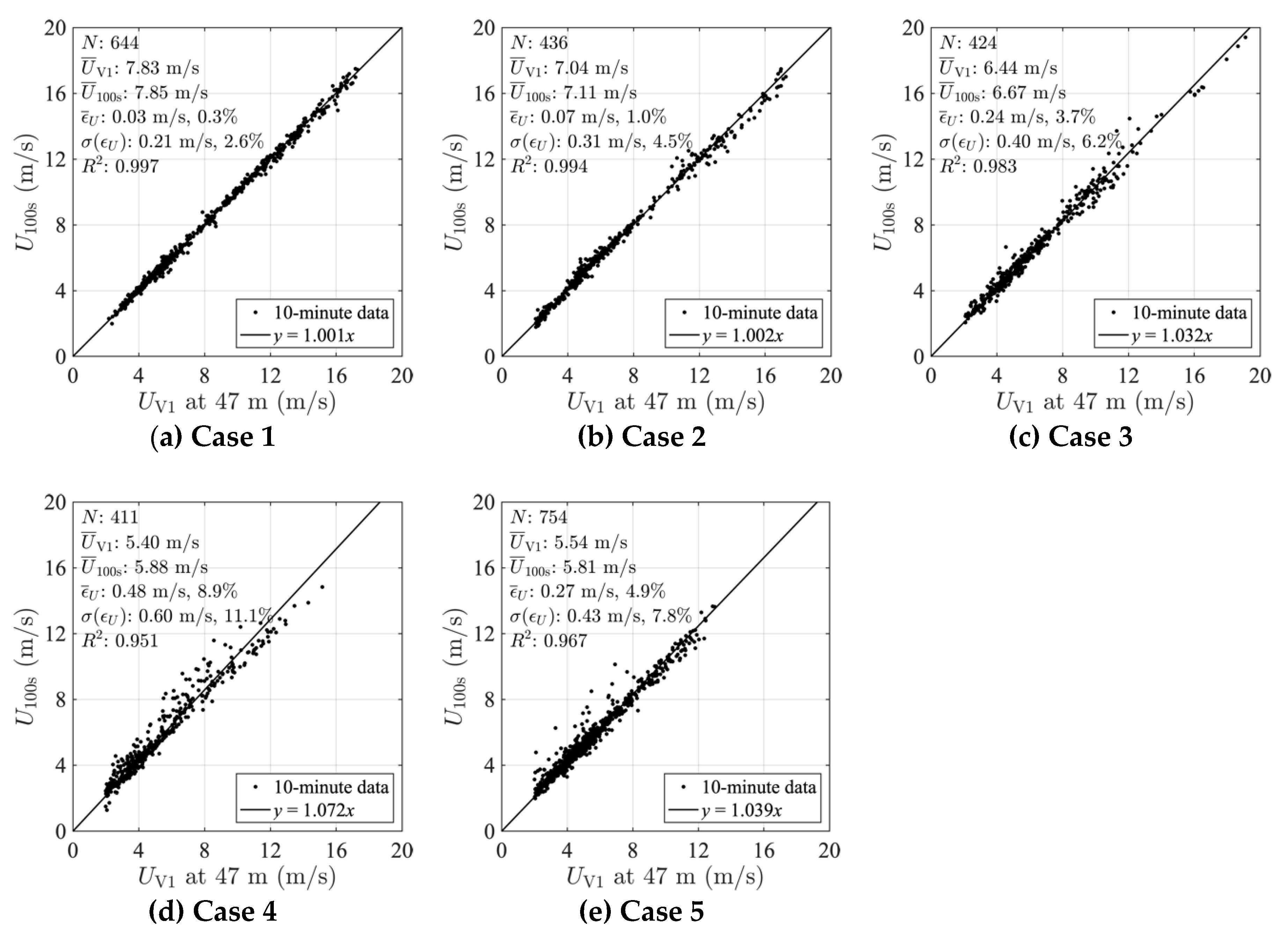
Figure 6 shows the scatter plots comparing wind speeds from the V1 () and 100s () for Cases 1–5. In order to quantitatively compare the accuracies between experiment cases, the deviations of the V1 and 100s wind speeds () were first calculated. The mean deviation and the standard deviation of the deviation were then computed. Table 3 presents the number of samples (), the mean wind speeds of the V1 () and 100s (), the mean deviation (), and the standard deviation of the deviation (). In addition, the coefficient of the regression line () and the determination coefficient () are also presented. For the mean deviation and the standard deviation, the relative values, which are normalized by the mean wind speeds of V1, are also given. In terms of the regression line, according to a previous study [10], one-parameter fitting was used for the validations of wind speed, while two-parameter fitting was used for the validations of wind direction.
The comparisons between the experiments with different azimuth ranges (Cases 1 to 4) show that the accuracy of the VVP-based wind speed retrieval was significantly affected by the azimuth angle range. The results for Case 1 and Case 2, which had azimuth angle ranges of 60° and 45°, were found to have good agreement with the V1 wind speeds. On the other hand, the measurement accuracy decreased as the azimuth range narrowed, as shown in the figures for Case 3 and Case 4. In Case 5, the settings are identical to those in Case 4 except for the scan rate. The slower scan rate in Case 5 was used to increase the number of radial wind speeds data in the curve fitting. It was found that the results for Case 5 were relatively improved compared to Case 4, but the points for this case were still more scattered than those for Case 1 and Case 2.
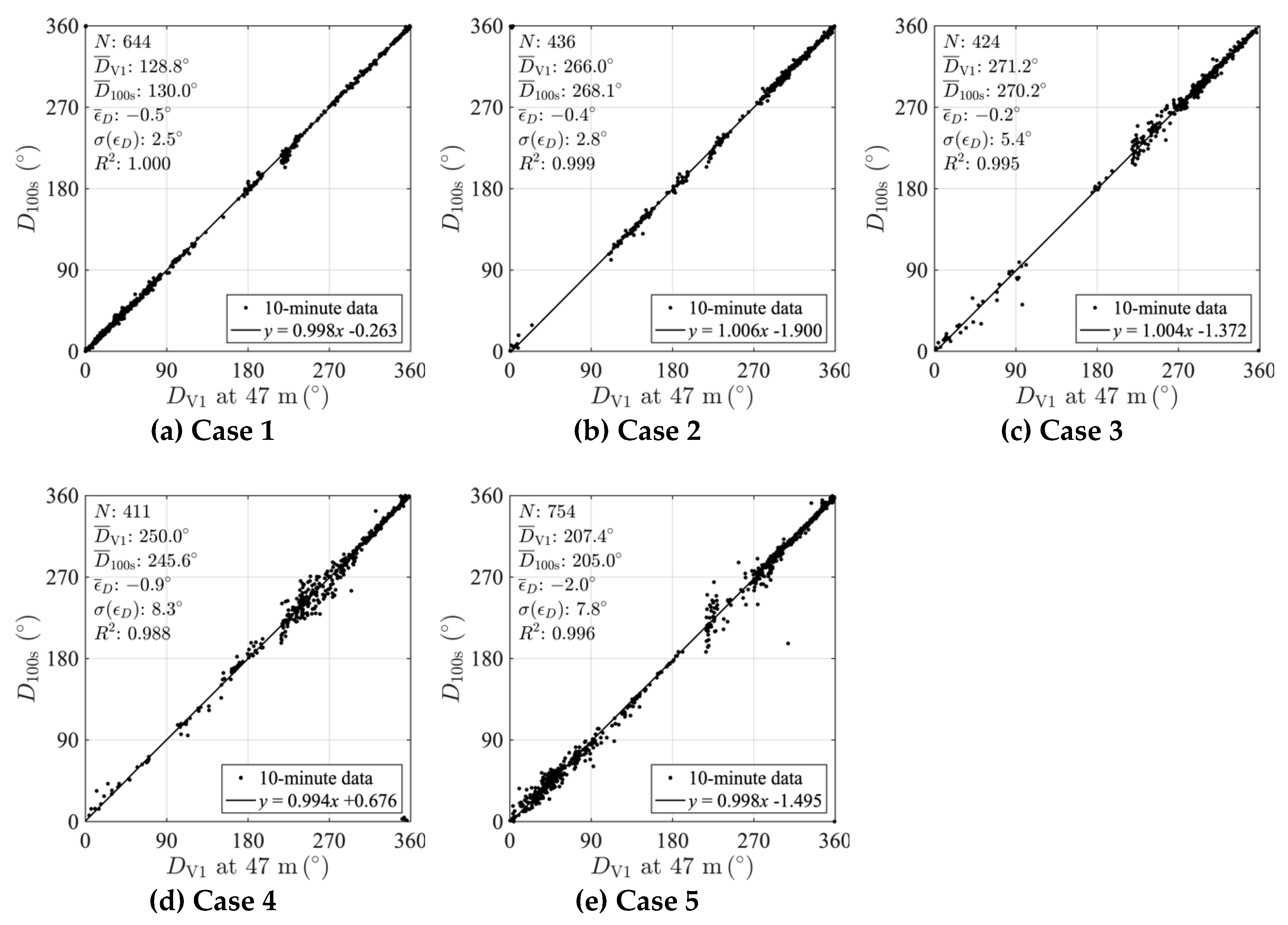
Figure 7 shows the wind direction plots. Here, and indicate the mean wind directions for V1 and 100s, respectively. The statistics for the mean wind direction for all of the experiments are described in Table 4. In calculating the error metrics for wind direction , , , and R2), the direction difference was limited to values between −180° and +180° to cancel the effect of periodicity between 0° and 360°. Similar to the results obtained for wind speeds, the wind direction accuracy of the 100s depended strongly on the azimuth range. When the azimuth ranges were less than 45°, the wind direction accuracy of the 100s decreased. A comparison between Case 4 ( = 3°/s) and Case 5 ( = 1°/s ) showed that decreasing the scan rate so that more radial wind speed data can be used for curve fitting did not improve the wind direction accuracy of the 100s.
Figure 6 and Figure 7 indicate that a wider azimuth angle produced better results for scanning LiDARs with the VVP method. The question arises as to how large of an azimuth angle is reasonable for wind resource assessment. In terms of LiDAR accuracy, previous studies [19,29] established acceptance criteria based on the International Electrotechnical Commission (IEC) standard 61400-12-1 [28], which included a technical note for remote sensing devices used for the power performance testing of wind turbines. Strictly speaking, the details of the criteria presented in the literature differ slightly. However, it is commonly accepted that for both wind speed and wind direction accuracy, the slope of the regression line should be between 0.98 and 1.02 and the determination coefficient should at least be greater than 0.98. Case 1 and Case 2 satisfy these acceptance criteria. The indication is that an azimuth width of more than 45° would be preferable for offshore wind measurements using the 100s and the VVP method.
3.2.2. Sensitivity to Elevation Angle Setting
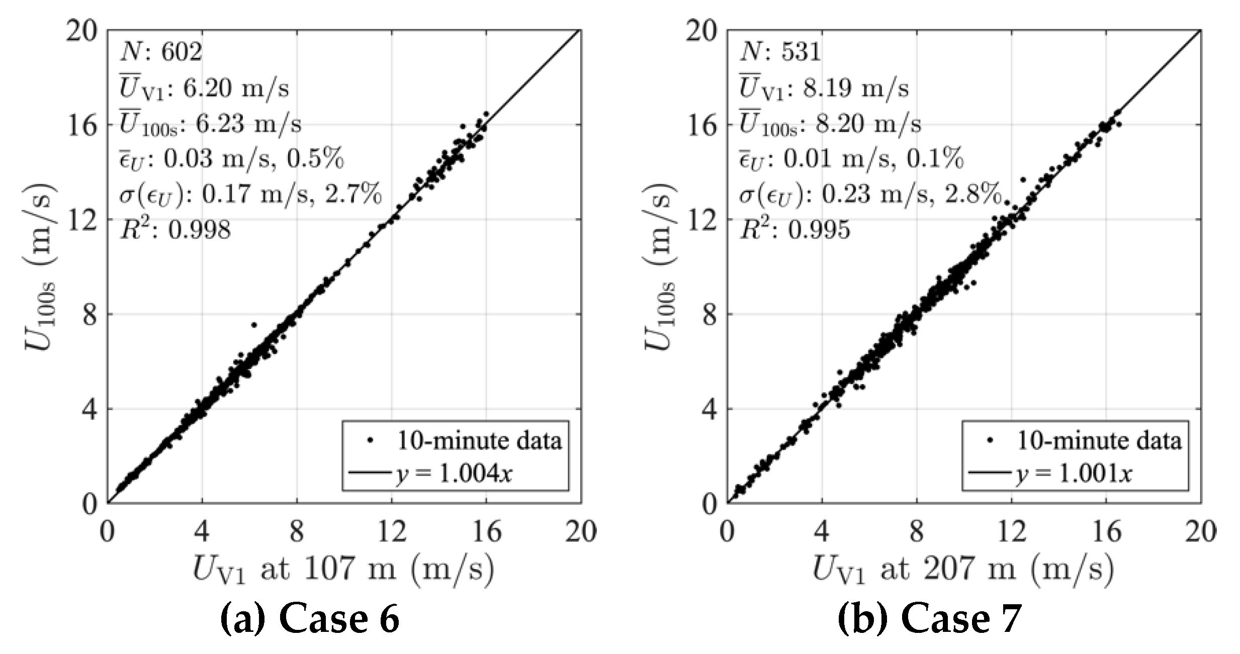
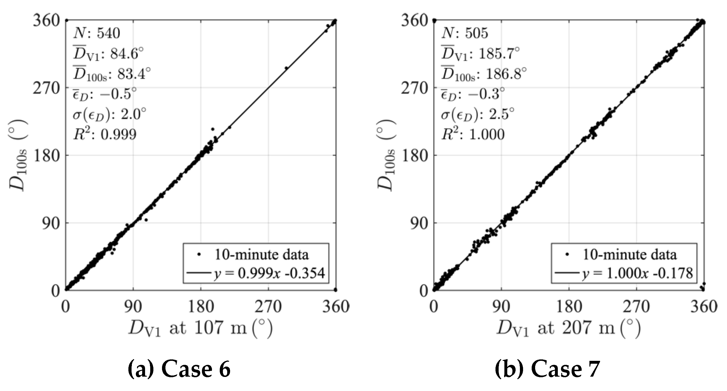
Figure 8 and Figure 9 show the scatter plots of the V1 and 100s wind speeds and directions for Case 6 ( = 14.11°) and Case 7 ( = 26.05°). The evaluation heights for Case 6 and Case 7 are 107 and 207 m ASL, respectively. The azimuth angle settings in these cases were identical to Case 2, i.e., φrange = 45°. The two-parameter fitting VVP, which ignores the vertical wind speed component (cf. Equation (6)) included in the original equation, was used for the analysis. Thus, if the vertical component of wind speeds was not negligibly small compared to the horizontal components, the accuracy of the wind speeds and directions should decrease as the elevation angle increases. However, these figures show that the accuracy of the 100s wind speeds and directions aloft did not deteriorate as the elevation angle increased. In fact, the accuracies for Case 6 and Case 7 increased in comparison to Case 2. This may be associated with the tendency of the wind to become more homogeneous at higher altitudes.
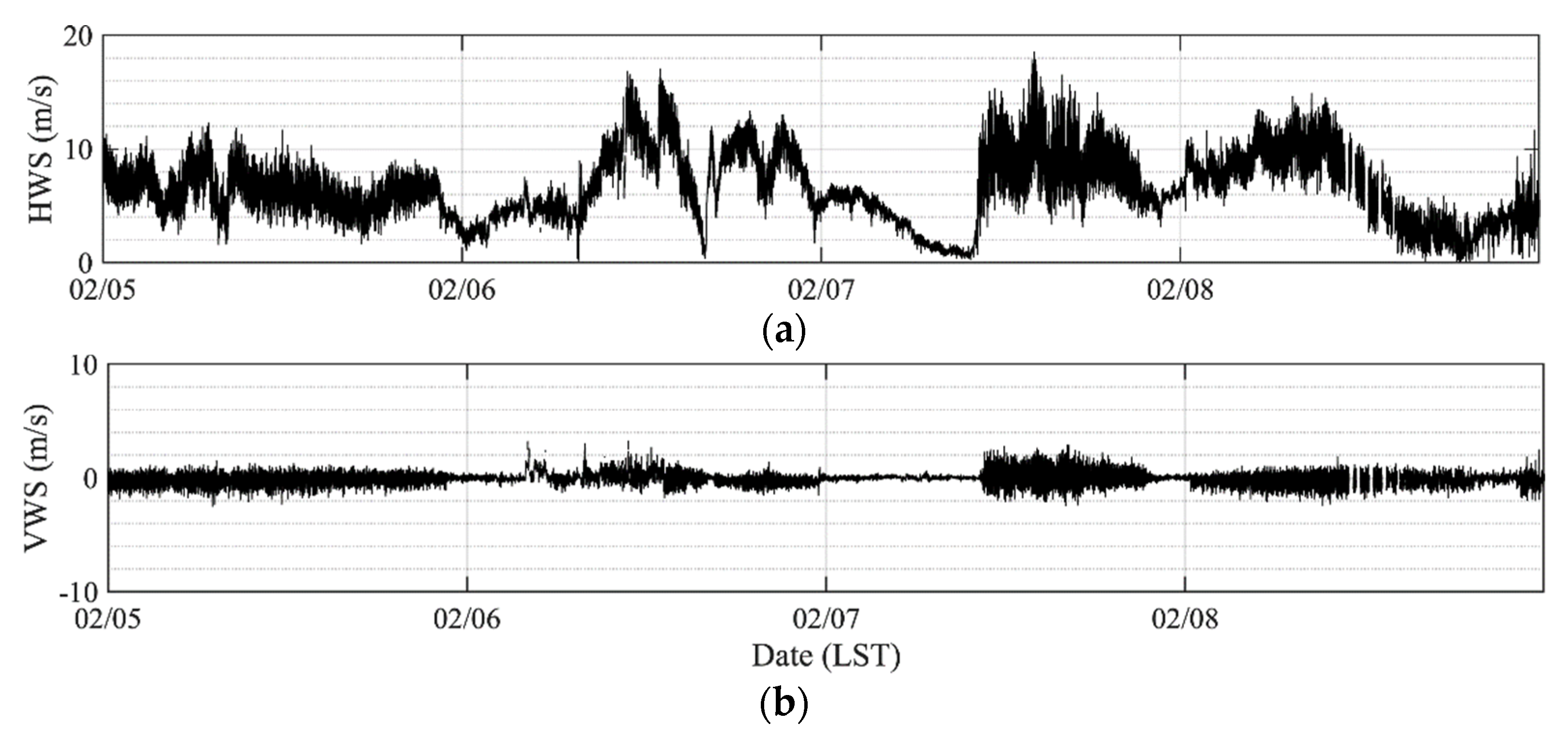
Figure 10 shows the time series of the horizontal and vertical wind speed components observed by V1 at a height of 107 m ASL for the period from 5 to 8 February 2019. The component of velocity was not directly observed by V1, as it is calculated from a transformation conversion of the line-of-sight wind speed using the DBS method. From Figure 10, it appears that the magnitude of is mostly less than 10% of the horizontal wind speed. Thus, these results indicate that neglecting the vertical wind speed component in the two-parameter fitting VVP is quite acceptable for measuring offshore winds, which have a small vertical wind speed component. Therefore, we concluded that the elevation angle setting between 5° and 26° did not produce any significant difference in the measurement accuracy for the same distance from the position of the scanning LiDAR.
3.2.3. Impact of Wind Direction on Wind Speed Accuracy
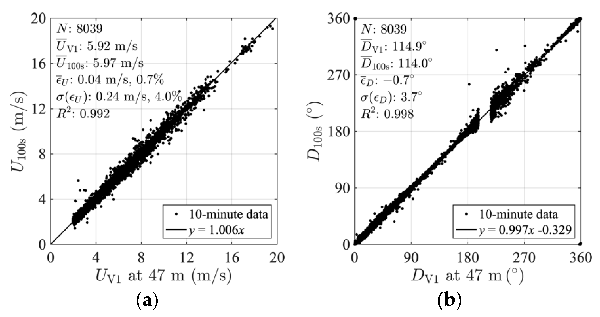
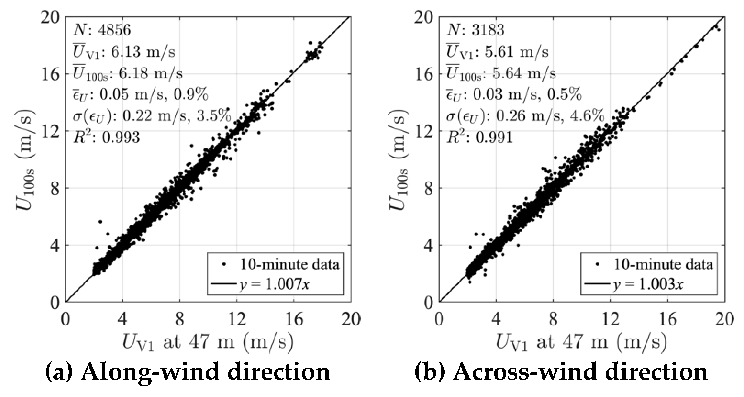
Previous studies [19] indicated that the accuracy of wind speeds obtained from a single scanning LiDAR were significantly affected by the wind direction. The accuracy of the wind speeds with an across-wind direction, defined as perpendicular to the LiDAR heading angle ±45°, might be lower than those with an along-wind direction, defined as parallel to the LiDAR heading angle ±45°(cf. Figure 3 for the definitions). In order to investigate the impact of wind direction on the accuracy of the retrieved horizontal wind speeds, an experiment with the same setting as Case 2 but covering a longer period of time (62 days) was conducted and is defined as Case 8 in Table 2.
Scatter plots of the V1 and 100s wind speeds and wind directions for Case 8 are shown in Figure 11. The 100s wind speeds have a mean deviation of 0.04 m/s (0.7%), a standard deviation of deviation of 0.24 m/s (4.0%), and a determination coefficient of 0.992; the 100s wind directions have a mean deviation of −0.7°, a standard deviation of deviation of 3.8°, and a determination coefficient of 0.998. To identify the impact of wind direction, Figure 12 shows two scatter plots for wind speed—one for along direction cases (as defined above) and one for across direction cases, based on the wind direction obtained from V1. As shown here, the results for the along-wind direction exhibit slightly better results in the standard deviation of the deviation, but no significant differences were observed between the two cases.
To investigate the influence of the wind direction in greater detail, the ratios of the V1 wind speeds and the 100s wind speeds were plotted as a function of the V1 wind direction at a height of 47 m (Figure 13). The bin-averaged values with a 5° bin width and the associated 1 standard deviation bounds were also plotted. The along and across direction classifications were indicated by the dark solid and dashed horizontal lines. The blue and red arrows, respectively, indicate wind blowing from the sea to the land and wind blowing from the land to the sea. As can be seen here, most of the bin-averaged values were plotted for directions between 335° and 145°, with the winds coming from the sea sectors, had a ratio close to 1.0. On the other hand, the bin-averaged ratios for directions between 155° and 325°, with the winds coming from the land sectors, were more widely scattered. The ratios between 175° and 230° were greatly scattered due to the influence from the nearby wind turbines. Thus, the accuracy of the wind speed measurements appears to be less sensitive to whether the wind is an along or across wind compared to whether the wind is an onshore or offshore wind. This result indicates how important a homogeneous wind field is to the accurate observation of horizontal wind speeds and directions using a scanning LiDAR with the VVP method.
3.3. Data Availability and Accuracy Indicators
Overall, the wind measurements using the 100s and the VVP method agreed with the V1 values in the current study. Our validation results suggest that using offshore wind measurements via a single scanning LiDAR would be a promising way to assess the nearshore wind conditions. However, the comparisons above were made with references located only 400 m from the scanning LiDAR position. In reality, the wind turbines would be situated a few kilometers off the coast even for nearshore wind farms. Accordingly, the data availability further offshore and the indicators for assessing the data quality were investigated by analyzing the CNR value and the goodness of fit obtained from the curve fitting in the VVP method.
3.3.1. CNR Variation on the Measurement Range
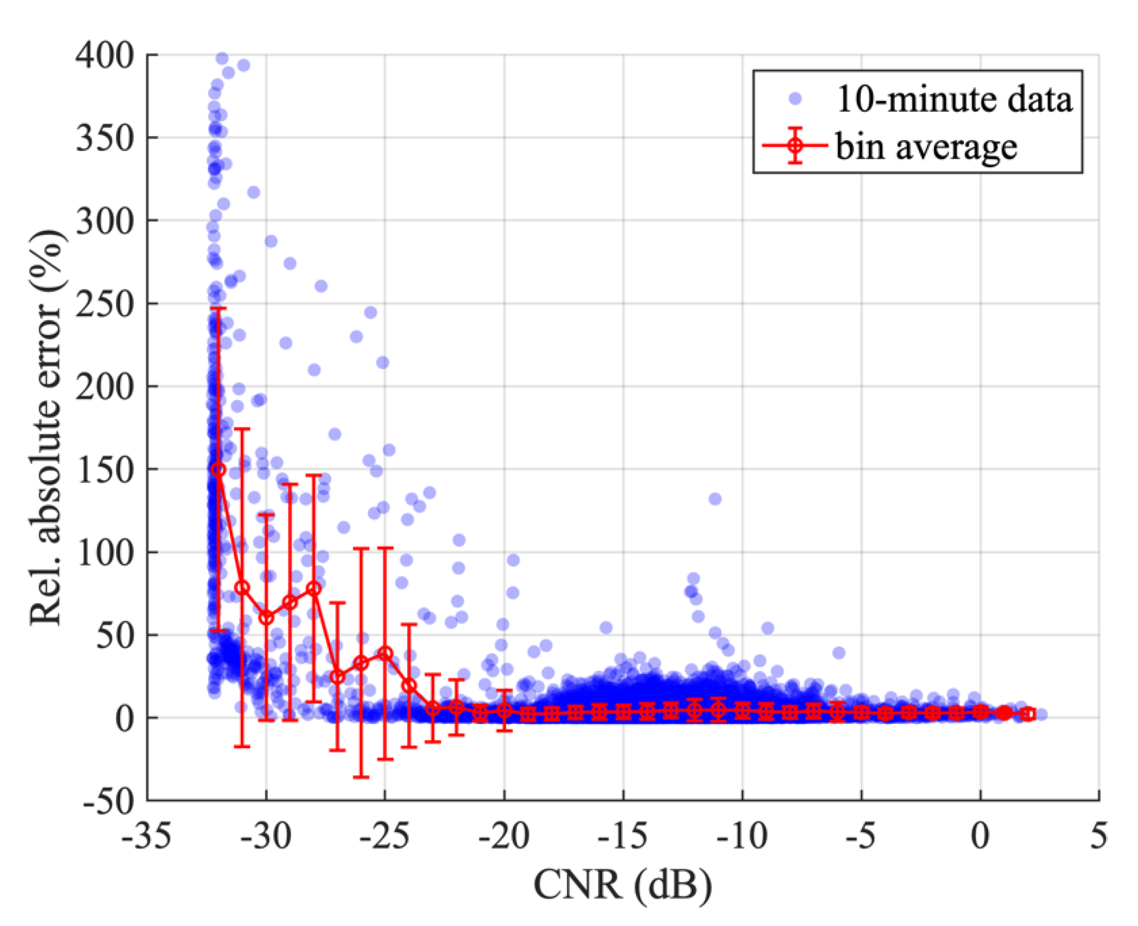
As shown in previous studies [30], the CNR can serve as a good indicator for evaluating the reliability of LiDAR-generated measurement data. Generally, the fraction of the unreliable contaminated data increased as the CNR value decreased. Before estimating the variation in data availability and accuracy associated with the measurement range, the relationship between the CNR value and the accuracy of the 100s wind speed were investigated. Here, the relative absolute errors (RAEs) for the 10-minute means were employed as an index of accuracy. The definition of RAE is given by
Figure 14 shows a plot of the RAEs for the 100s as a function of the CNR values for Case 8. The red circles and error bars indicate the bin-averaged and the standard deviation values, respectively. As expected, the CNR values were obviously correlated with the RAEs. The accuracy of the 100s tended to gradually decline, as the CNR took on values below −23 dB. The accuracy worsened significantly when the CNR value fell below −30 dB.
Figure 15 shows the frequency distribution of the CNR values for measurement ranges from 500 to 3000 m as determined from the Case 8 data collected over a three-month period. As shown, the peak frequency in the CNR distribution at a 500 m range occurred around −15 dB. As the distance increased, the peak frequency shifted toward lower CNR values. The CNR distribution for the 3000 m distance had one peak around −25 dB and the other smaller peak around −33 dB. While it is preferable to set a higher CNR threshold to increase the quality of data used for actual assessment, a higher CNR threshold will reduce the data availability, especially further away from the LiDAR position. For example, if a CNR value of −30 dB is used as the data reliability threshold, 33% of the raw measurements at a distance of 3000 m should be excluded from the analysis. The greatest number of usable observations are available at the 500 m distance.
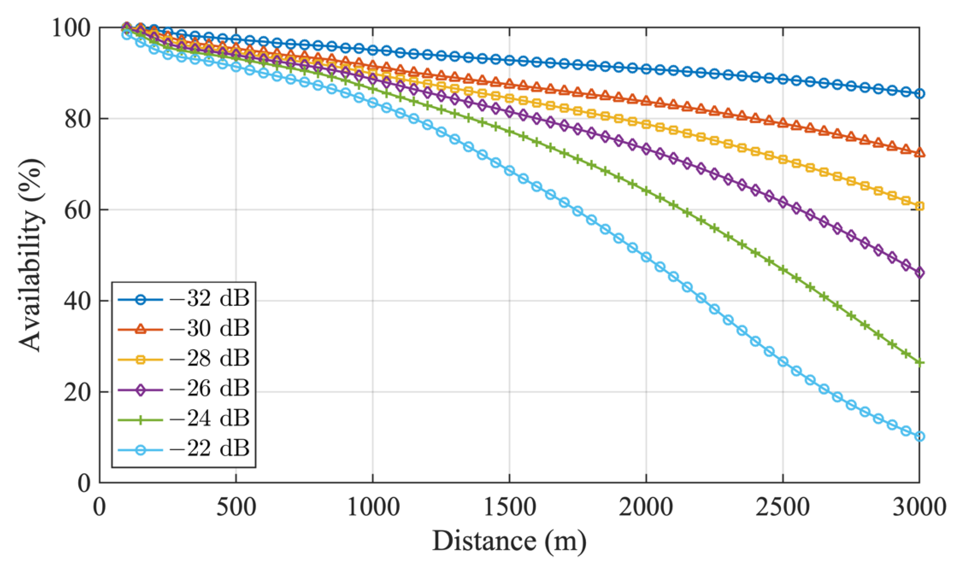
Figure 16 shows the data availability for various CNR thresholds as a function of the distance from the 100s for Case 8. As illustrated in the figure, the CNR threshold of −30 dB was set, and we can expect data availability of 85%, 80%, and 70% at distances of 2000, 2500, and 3000 m, respectively. According to the report from the Carbon Trust on the acceptance criteria for floating LiDAR technologies [10], a data availability of 85% is required in order to qualify as an acceptable method to tradition measurement with met masts. Given this requirement, a distance of 2000 m would appear to be the maximum effective range for the application of offshore wind measurements using the current scanning LiDAR. The CNR variation along the measurement range is likely influenced by factors including the specific device, height, and atmospheric conditions.
3.3.2. Goodness of Fit for the Curve Fitting
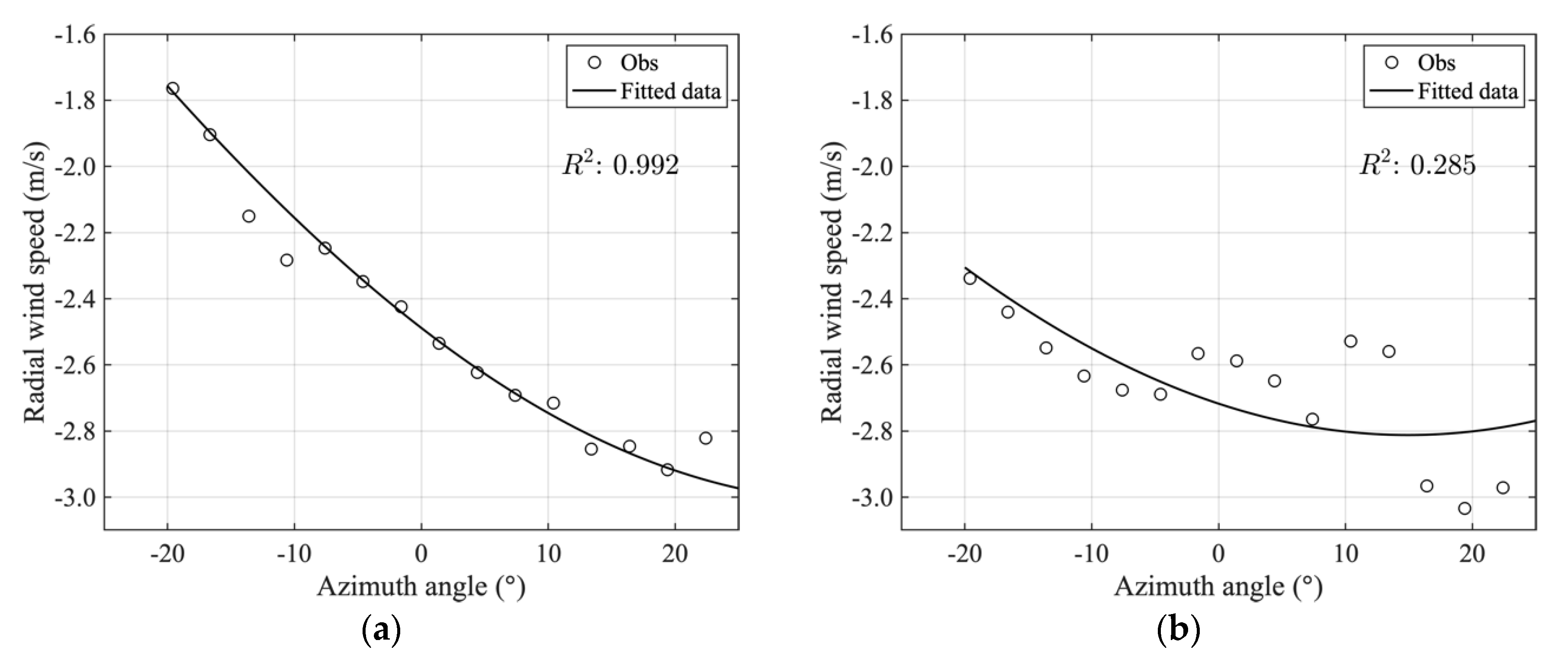
As well as the CNR value, the quality of the curve fitting is an indicator for investigating the accuracy of the retrieved velocities with the VVP method. For this examination, we analyzed the goodness of fit for the curve fitting performed for the VVP method. Figure 17 shows the instantaneous value of the radial wind speed and fitted curve for two illustrative cases. In one, the determination coefficient was relatively high (0.992), while in another it was relatively low (0.285). Cases in which the determination coefficient is close to 1.0 are compatible with the assumption used in the VVP method—that the wind field is homogeneous in time and space—whereas cases in which the coefficient value is low are not.
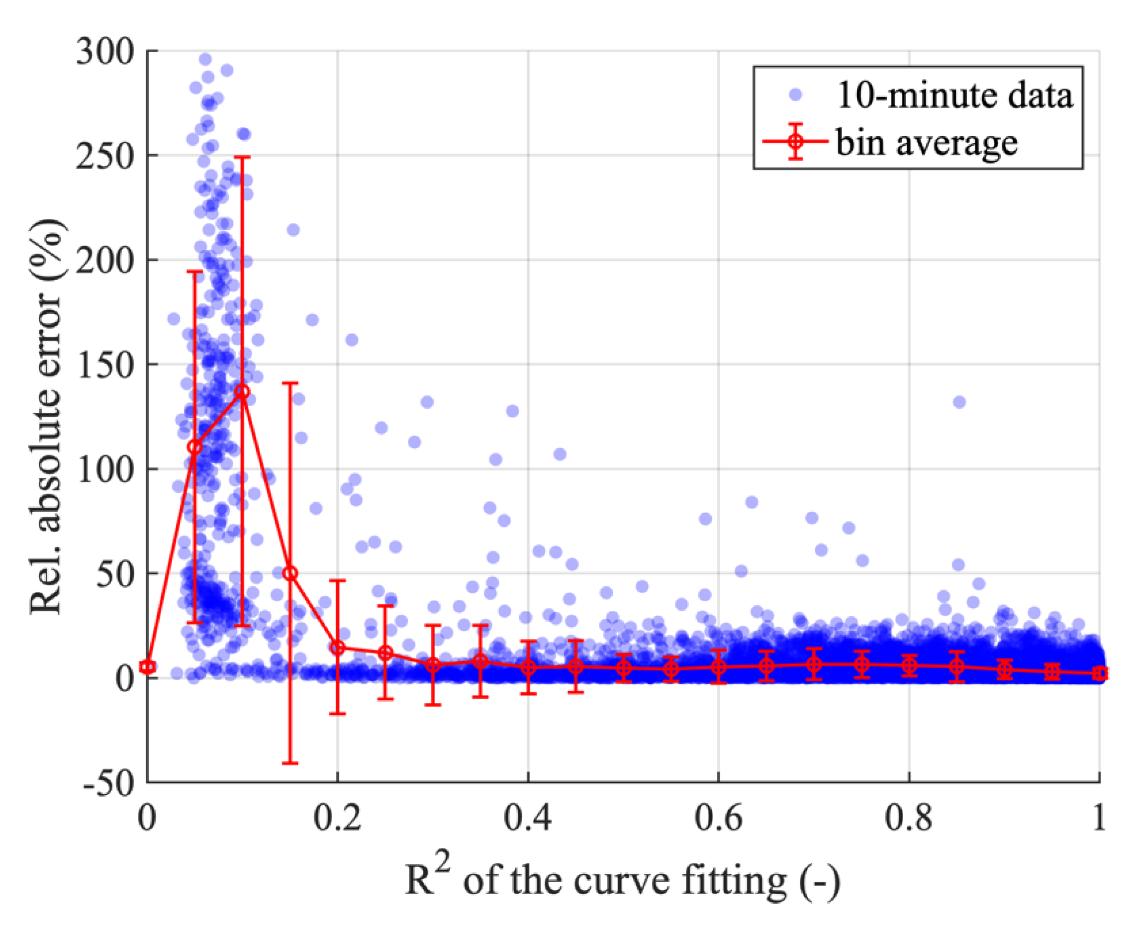
Similar to the analysis of the relationship between the CNR values and the accuracy of the wind speed measurement (cf. Figure 14), the relationship between the RAE and the coefficient of determination () for Case 8 was investigated and the results are presented in Figure 18. The red circles with error bars in Figure 18 indicate the bin-averaged values and their standard deviation. As can be seen here, the RAE values increase rapidly when the value of falls below 0.2. This result indicates that if the quality of the curve fitting decreases, the accuracy of the measurements also decreases. In other words, the determination coefficient derived from the curve-fitting process serves as an indicator for estimating the quality of the horizontal wind speed measurements using a single scanning LiDAR with the VVP method.
4. Discussion
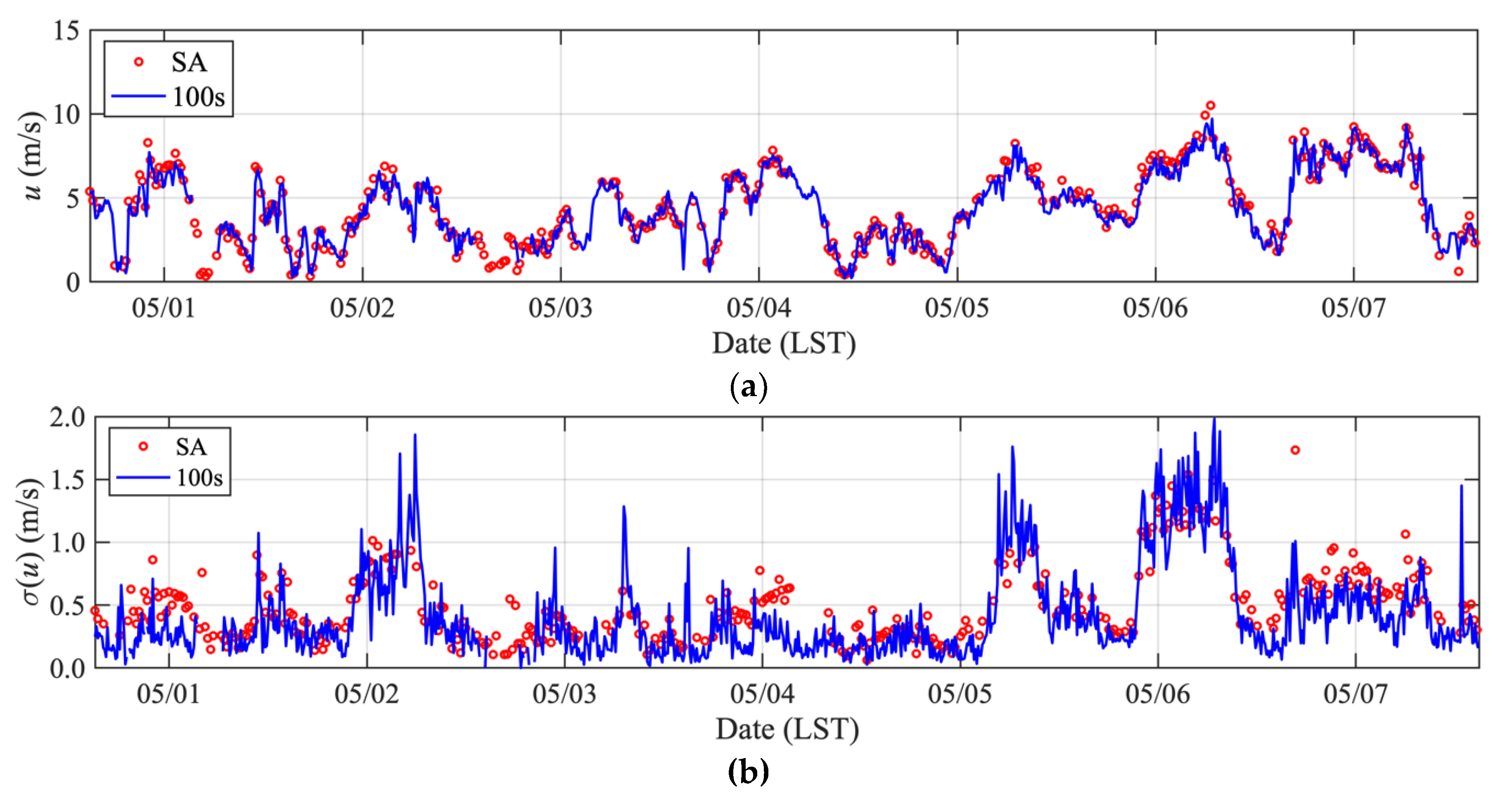
For assessing offshore wind conditions, in addition to the mean wind speeds and wind directions, the accuracy of the turbulence intensity (TI) measurements using a scanning LiDAR is also crucial. This parameter is tightly associated with wind turbine design. We discussed the applicability of a single scanning LiDAR for TI measurements by comparing the observations from the 100s with those from the SA at a height of 10 m ASL. Figure 19 shows the time series of the 10-minute mean and standard deviation of wind speed values from the SA and 100s for the period of one week from 1 to 7 May 2019. This corresponds to Case 9 in Table 2. As the SA measurements were strongly influenced by the presence of the neighboring observational hut, observations with wind directions between 49° and 89° were excluded from the analysis.
The match between the time series of the mean wind speeds recorded by the 100s and the time series of the mean wind speeds recorded by the SA was not quite as good as it was for the 100s–V1 comparisons. In comparing the mean 100s wind speeds to the mean SA wind speeds, we found that the 100s wind speeds compared to the SA wind speeds had a mean deviation of −0.17 m/s (−3.4%) and a standard deviation of 0.55 m/s (10.8%), and the linear regression equation was y = 0.959x, with a determination coefficient of 0.963. The comparatively poor match may be due to the non-homogeneous nature of the wind field near the surface.
Figure 19 indicates that measuring the standard deviations of wind speeds with scanning LiDARs was more challenging than measuring the 10-minute mean wind speeds. We found that, for a time scale of 2 h, the standard deviation of the 100s values followed a trend similar to that of the standard deviations obtained from the SA. However, large differences were observed for the shorter time scales. The sonic anemometer used in this study had a 0.25-second temporal interval (= 4 Hz), while the 100s required approximately 15 s (= 0.067 Hz) to measure horizontal wind speeds and directions with the VVP method. As a result, the 100s collected only 40 samples in a 10-minute duration, while the SA collected 2400 samples during the same time. This difference may explain why the 100s time series of standard deviation values shows greater fluctuations than that the SA time series, as well as the difference in the measurement volumes between the 100s and SA.
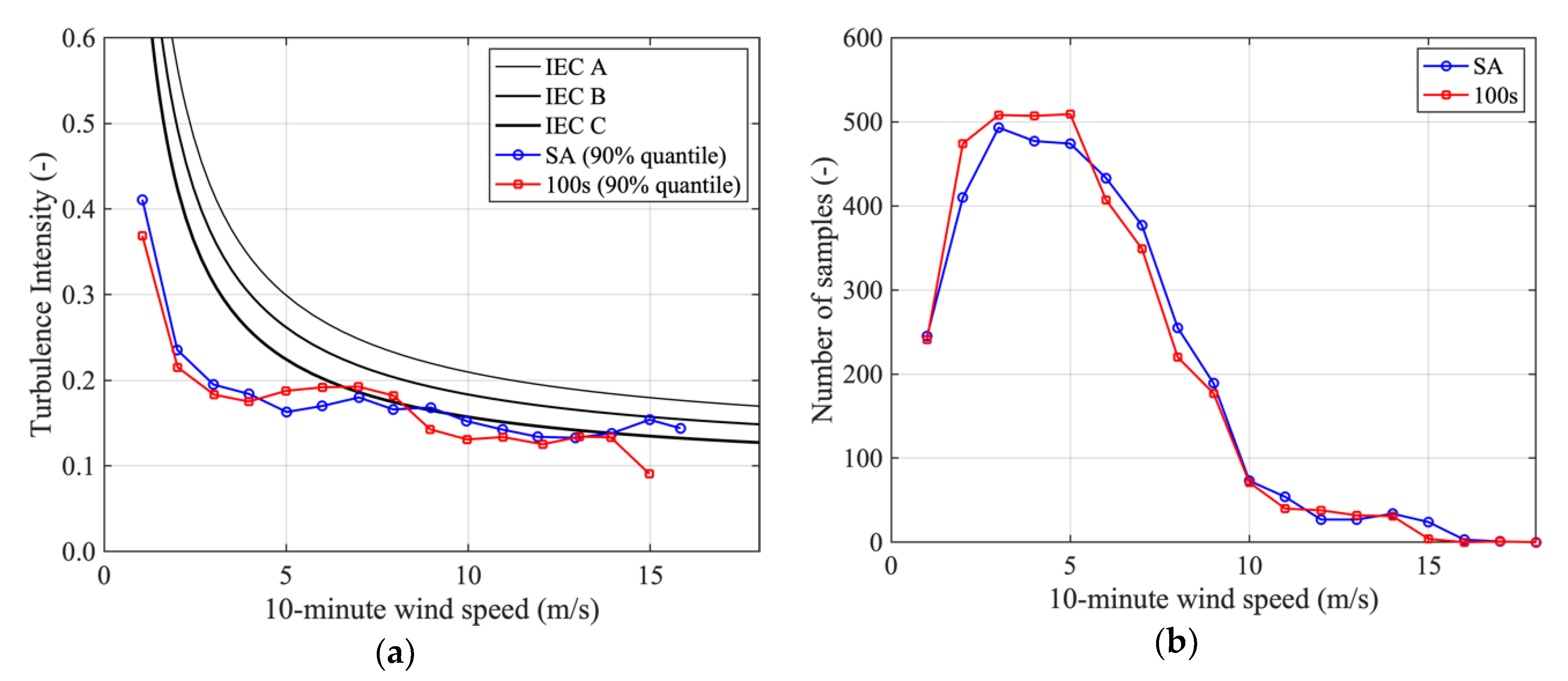
The accuracy of the standard deviations obtained from the 100s was worse than that of the mean wind speeds. However, the instantaneous values of the standard deviation of wind speeds are not directly used for wind turbine design. In practice, TI, which is the 10-minute standard deviation of wind speed, normalized by the mean wind speed, is first calculated. The 90% quantile values of TI with a bin width of 1 or 2 m/s are then plotted as a function of the mean wind speed to evaluate the turbulence condition. Figure 20a shows the relationships between the 10-minute mean wind speed and TI of the SA and 100s for Case 9. The dark lines indicate the IEC standards [30] for classifying wind turbines based on site-specific turbulence conditions. The number of samples for each bin is shown in Figure 20b.
The TI values produced by the 100s were slightly larger than those by the SA for mean wind speeds in the range of 5–8 m/s; for a mean wind speed of 9–11 m/s, the 100s values were lower. We found that the difference between the SA and 100s values was comparable to or less than the difference between the IEC categories for most ranges. Given that the comparisons here were with an SA installed near the surface, the accuracy of the standard deviation measurements for the 100s at the height of a wind turbine hub might well improve, as might the accuracy of the mean wind speeds and directions. Consequently, the turbulence intensity obtained from the 100s with the VVP method would appear to have potential as an alternative to in situ wind measurements using meteorological masts. However, this is just a speculation based on the data from two months. The accuracy of the TI measurements from a single scanning LiDAR would be impacted by the scanning configurations. Thus, further investigations are necessary to reach any conclusions regarding the accuracy of scanning LiDAR-measured turbulence intensity at the hub height level of utility scale wind turbines.
5. Conclusions
This study investigated the accuracy of offshore wind speed measurements using a single scanning LiDAR and a two-parameter curve-fitting VVP method. The accuracies of the 10-minute mean wind speeds and directions at heights of 47, 107, and 207 m ASL, that were obtained from a scanning LiDAR positioned at the water’s edge, were quantitatively examined by comparing the scanning LiDAR values to observations from a vertical profiling LiDAR. The accuracy of the LiDAR-generated turbulence intensity value, which is a parameter used in wind turbine design, was also investigated by comparing the scanning LiDAR values with the observations from an SA mounted on the pier. A methodology for estimating the pitch and roll angles of the instrument after deployment was also described. The results obtained from the experiments can be summarized as follows:
In Case 1, the 100s mean wind speeds were found to have a mean deviation of 0.03 m/s (0.3% of the mean value), a standard deviation of deviation of 0.21 m/s (2.6%), and a determination coefficient of 0.997. The 100s wind direction values were found to have a mean deviation of −0.5°, a standard deviation of deviation of 2.5°, and a determination coefficient of 1.000. These values satisfied the criteria used in vertical and floating LiDAR verification by the IEC. We also investigated the influences of the azimuth width on the wind speed and direction accuracy. As a result, the accuracy of the 100s was found to decline with decreases in the azimuth width (Cases 2–4). In Case 5, an attempt was made to improve the accuracy by decreasing the scan rate for a smaller azimuth range. However, we found that this did not increase the accuracy. An azimuth width of more than 45° was preferred for use with the VVP method.
During a three-month long validation (Case 8), the impact of the wind direction on the accuracy of the wind speed retrievals was investigated. Previous studies indicated that the accuracy for winds in the across-wind sectors (winds perpendicular to the LiDAR heading angle) was worse than that for winds in the along-wind sectors (winds parallel to the LiDAR heading angle). However, we found no clear differences in wind speed accuracy between the sectors. The measurement accuracy differences between the land- and sea-sector winds were also examined. We found that the wind speed measurements for the sea sector showed distinctly better results. The poorer results for the land sector may be due to the non-homogeneous wind field induced by the land surface.
We also investigated the impact of the elevation angle. The results from the relevant cases (Case 6 and Case 7) showed that the wind speed obtained from the 100s was insensitive to the elevation angle setting. This may be due to the vertical wind speed being negligibly small compared to the horizontal wind speed in coastal areas. We also found that the accuracy of the wind speed and direction increased as the height increased. The wind speed at the height of 107 m ASL had a mean bias of 0.03 m/s (0.5%) and a determination coefficient of 0.998, while the (less accurate) wind speeds measured near the surface showed a mean deviation of −0.18 m/s (−3.5%) and a determination coefficient of 0.963 against the SA observations. The wind field near the surface is likely to be much more disturbed by surface factors, which can result in large variations in the wind conditions in time and space. Our results suggest that the more homogeneous wind field near the hub height of a wind turbine would be compatible with the homogeneity assumption in the VVP method.
In addition, the data availability and indicators for the data quality were investigated by analyzing the CNR value and the determination coefficients calculated in the curve-fitting process of the VVP method. We first confirmed that the CNR value was closely associated with the accuracy of the measurements by making comparisons with the vertical profiling LiDAR observations. The additional analysis for Case 8 showed that we can expect a data availability level of 85%, 80%, and 70% at distances of 2000, 2500, and 3000 m, respectively, if we employ a CNR value of −30 dB as the threshold for the data reliability index. We also confirmed that the determination coefficient was connected with the measurement accuracy. The determination coefficient obtained via the curve fitting process in the VVP method was an additional indicator for assessing the data quality.
Finally, we also examined the measurement accuracy of TI by comparing the scanning LiDAR-based measurements with the SA measurements near the surface in Case 9. We found that the differences between the standard deviations of the SA and 100s wind speeds were much larger than the differences between the 10-minute mean wind speeds and directions. Due to the coarse temporal resolution and large measurement volume of the 100s, the 10-minute standard deviations from the 100s were expected to be more scattered than those from the SA. In addition, the 90% quantiles of the standard deviations for the SA and 100s measurements were compared. As a result, the difference in the TI was less than the difference between the IEC standard categories. Thus, we found that using a single scanning LiDAR for offshore wind measurements had potential not only for wind resource assessment but also for assessing the site-specific conditions considered in wind turbine design.
Overall, the offshore wind measurements using a single scanning LiDAR with the VVP method showed good performance when compared to the reference observations obtained at a distance of 400 m from the scanning LiDAR. An attempt to evaluate the data availability further offshore showed that this measurement method would be equally as accurate within a range from 2000 to 2500 m. Accordingly, we argue that using a single scanning LiDAR with the VVP offers a promising and cheaper alternative to in situ observations using offshore meteorological masts and floating LiDAR technologies. For future research, we plan to conduct measurement campaigns with an offshore met mast and a vertical profiling LiDAR located 2 to 3 km away from the two scanning LiDARs installed on the coast to compare the performance with dual LiDAR measurements.
Author Contributions
Conceptualization, S.S. and J.P.G.; Data curation, S.S., J.P.G., T.O., T.K. and S.N.; Funding acquisition, S.S. and T.K.; Methodology, S.S. and J.P.G.; Project administration, S.S.; Writing—original draft, S.S. and J.P.G.; Writing—review and editing, T.O., T.K. and S.N. All authors have read and agreed to the published version of the manuscript.
Funding
This work was supported by the Japan Society for the Promotion of Science (JSPS) KAKENHI Grant Number 17H03492. This research was also supported by an international collaboration project for energy technologies funded by the Japanese Ministry of Economy, Trade and Industry (METI).
Conflicts of Interest
The authors declare no conflict of interest.
Abbreviations
| 100s | Windcube 100s |
| ASL | Above Sea Level |
| CNR | Carrier-to-Noise Ratio |
| DBS | Doppler Beam Swinging |
| HORS | Hazaki Oceanographic Research Station |
| HTC | Hard Target Calibration |
| IEC | International Electrotechnical Commission |
| LiDAR | Light Detection and Ranging |
| METI | Ministry of Economy, Trade and Industry |
| PPI | Plan Position Indicator |
| RAE | Relative Absolute Error |
| RHI | Range Height Indicator |
| SA | Sonic Anemometer |
| STC | Soft Target Calibration |
| TI | Turbulence Intensity |
| V1 | Windcube V1 |
| VVP | Velocity Volute Processing |
References
- Global Wind Energy Council (GWEC). Global Wind Report 2019; GWEC: Maharashtra, India, 2019. [Google Scholar]
- METI. Promising Sea Areas and Sites Selected for Targeted Promotion. Available online: https://www.meti.go.jp/english/press/2019/0730_001.html (accessed on 12 August 2019).
- Barthelmie, R.J.; Wang, H.; Doubrawa, P.; Pryor, S. Best Practice for Measuring Wind Speeds and Turbulence Offshore through In-Situ and Remote Sensing Technologies; Report to the Department of Energy as Partial Fulfilment of Grant EE0005379; Cornell University: Ithaca, NY, USA, 2016. [Google Scholar]
- Goit, J.P.; Shimada, S.; Kogaki, T. Can LiDARs Replace Meteorological Masts in Wind Energy? Energies 2019, 12, 3680. [Google Scholar] [CrossRef] [Green Version]
- Hasager, C.B.; Sjoholm, M. Editorial for the Special Issue “Remote Sensing of Atmospheric Conditions for Wind Energy Applications”. Remote Sens. 2019, 11, 781. [Google Scholar] [CrossRef] [Green Version]
- Sathe, A.; Banta, R.; Pauscher, L.; Vogstad, K.; Schlipf, D.; Wylie, S. Estimating Turbulence Statistics and Parameters from Ground-and nAcelle-Based Lidar Measurements: IEA Wind Expert Report; DTU Wind Energy: Roskilde, Denmark, 2015. [Google Scholar]
- Shimada, S.; Takeyama, Y.; Kogaki, T.; Ohsawa, T.; Nakamura, S. Investigation of the Fetch Effect Using Onshore and Offshore Vertical LiDAR Devices. Remote Sens. 2018, 10, 1408. [Google Scholar] [CrossRef] [Green Version]
- Shimada, S.; Takeyama, Y.; Kogaki, T.; Ohsawa, T.; Nakamura, S.; Kawaguchi, K. Enhanced offshore wind simulations with WRF using LiDAR observation nudging. J. JWEA 2018, 42, 17–24. (In Japanese) [Google Scholar]
- Leosphere. Scanning Windcube. Available online: https://www.leosphere.com (accessed on 11 March 2020).
- Carbon Trust. Roadmap for the Commercial Acceptance of Floating LiDAR Technology; Carbon Trust: London, UK, 2018. [Google Scholar]
- Gottschall, J.; Wolken-Mohlmann, G.; Viergutz, T.; Lange, B. Results and conclusions of a floating-lidar offshore test. Enrgy Procedia 2014, 53, 156–161. [Google Scholar] [CrossRef]
- Hsuan, C.-Y.; Tasi, Y.-S.; Ke, J.-H.; Prahmana, R.A.; Chen, K.-J.; Lin, T.-H. Validation and Measurements of Floating LiDAR for Nearshore Wind Resource Assessment Application. Energy Procedia 2014, 61, 1699–1702. [Google Scholar] [CrossRef] [Green Version]
- Fuertes, F.C.; Iungo, G.V.; Porte-Agel, F. 3D Turbulence Measurements Using Three Synchronous Wind Lidars: Validation against Sonic Anemometry. J. Atmos. Ocean Technol. 2014, 31, 1549–1556. [Google Scholar] [CrossRef]
- Mann, J.; Cariou, J.P.; Courtney, M.S.; Parmentier, R.; Mikkelsen, T.; Wagner, R.; Lindelow, P.; Sjoholm, M.; Enevoldsen, K. Comparison of 3D turbulence measurements using three staring wind lidars and a sonic anemometer. Meteorol. Z. 2009, 18, 135–140. [Google Scholar] [CrossRef]
- Newsom, R.K.; Berg, L.K.; Shaw, W.J.; Fischer, M.L. Turbine-scale wind field measurements using dual-Doppler lidar. Wind Energy 2015, 18, 219–235. [Google Scholar] [CrossRef]
- Pena, A.; Mann, J. Turbulence Measurements with Dual-Doppler Scanning Lidars. Remote Sens. 2019, 11, 2444. [Google Scholar] [CrossRef] [Green Version]
- Newman, J.F.; Bonin, T.A.; Klein, P.M.; Wharton, S.; Newsom, R.K. Testing and validation of multi-lidar scanning strategies for wind energy applications. Wind Energy 2016, 19, 2239–2254. [Google Scholar] [CrossRef]
- Wagner, R.; Vignaroli, A.; Courtney, M.; McKeown, S.; Cussons, R.; Murthy, R.K.; Boquet, M. Real world offshore power curve using nacelle mounted and scanning Doppler lidars. In Proceedings of the EWEA Offshore 2015, Copenhagen, Denmark, 10–12 March 2015. [Google Scholar]
- Cameron, L.; Clerc, A.; Feeney, S.; Stuart, P. Remote Wind Measurements Offshore Using Scanning LiDAR Systems; OWA Report; Carbon Trust: London, UK, 2014. [Google Scholar]
- Courtney, M.; Wagner, R.; Murthy, R.K.; Boquet, M. Optimized Lidar Scanning Patterns for Reduced Project Uncertainty. In Proceedings of the EWEA 2014, Barcelona, Spain, 10–13 March 2014. [Google Scholar]
- Coutts, E.; Oldroyd, A.; Stein, D.; Boque, M.; Krishna, R.; Akhoun, M.; Espin, F.; Miguel Gonzalez Garcia, L. Cost Effective Offshore Wind Measurement. In Proceedings of the EWEA Resource Assessment 2015, Helsinki, Finland, 2–3 June 2015. [Google Scholar]
- Simon, E.; Courtney, M. A Comparison of Sector-Scan and Dual Doppler Wind Measurements at Høvsøre Test Station—One Lidar or Two? Technical Report DTU Wind Energy E-0112 (EN); DTU Wind Energy: Roskilde, Denmark, 2016. [Google Scholar]
- PARI. Hazaki Oceanographical Research Station (HORS). Available online: https://www.pari.go.jp/unit/edosy/en/main-facility/2.html (accessed on 10 September 2019).
- Calhoun, R.; Heap, R.; Princevac, M.; Newsom, R.; Fernando, H.; Ligon, D. Virtual towers using coherent Doppler lidar during the Joint Urban 2003 dispersion experiment. J. Appl. Meteorol. Clim. 2006, 45, 1116–1126. [Google Scholar] [CrossRef]
- Zhou, S.H.; Wei, M.; Wang, L.J.; Zhao, C.; Zhang, M.X. Sensitivity Analysis of the VVP Wind Retrieval Method for Single-Doppler Weather Radars. J. Atmos. Ocean Technol. 2014, 31, 1289–1300. [Google Scholar]
- Waldteufel, P.; Corbin, H. On the Analysis of Single-Doppler Radar Data. J. Appl. Meteorol. 1979, 18, 532–542. [Google Scholar] [CrossRef]
- Koscielny, A.J.; Doviak, R.J.; Rabin, R. Statistical Considerations in the Estimation of Divergence from Single-Doppler Radar and Application to Pre-Storm Boundary-Layer Observations. J. Appl. Meteorol. 1982, 21, 197–210. [Google Scholar] [CrossRef] [Green Version]
- International Electrotechnical Commision (IEC). IEC 61400-12-1 Wind Energy Generation Systems—Part 12-1: Power Performance Measurements of Electricity Producing Wind Turbines, 2nd ed.; IEC Central Office: Geneva, Switzerland, 2017. [Google Scholar]
- Hasager, C.B.; Stein, D.; Courtney, M.; Pena, A.; Mikkelsen, T.; Stickland, M.; Oldroyd, A. Hub Height Ocean Winds over the North Sea Observed by the NORSEWInD Lidar Array: Measuring Techniques, Quality Control and Data Management. Remote Sens. 2013, 5, 4280–4303. [Google Scholar] [CrossRef] [Green Version]
- Gryning, S.E.; Floors, R. Carrier-to-Noise-Threshold Filtering on Off-Shore Wind Lidar Measurements. Sensors 2019, 19, 592. [Google Scholar] [CrossRef] [PubMed] [Green Version]
Figure 1.
Experimental setup.

Figure 2.
Snapshot of the carrier-to-noise ratio (CNR) distribution obtained from the 100s with an azimuth width of 45° and an elevation angle of 0° for the period 2019-05-11 09:05:33 to 09:05:47 LST.
Figure 2.
Snapshot of the carrier-to-noise ratio (CNR) distribution obtained from the 100s with an azimuth width of 45° and an elevation angle of 0° for the period 2019-05-11 09:05:33 to 09:05:47 LST.

Figure 3.
Measurement of horizontal and vertical positions of the radial wind speed for Case 1. The red square indicates the location of the 100s. The pie chart shows the definition of the along and across wind direction sectors.
Figure 3.
Measurement of horizontal and vertical positions of the radial wind speed for Case 1. The red square indicates the location of the 100s. The pie chart shows the definition of the along and across wind direction sectors.

Figure 4.
Time series of (a) wind speeds and (b) wind directions obtained from V1 at a height of 107 m above sea level (ASL) for the period from January to September 2019 at Hazaki Oceanographical Research Station (HORS).
Figure 4.
Time series of (a) wind speeds and (b) wind directions obtained from V1 at a height of 107 m above sea level (ASL) for the period from January to September 2019 at Hazaki Oceanographical Research Station (HORS).

Figure 5.
Distributions of (a) the wind speeds and (b) wind directions at a height of 107 m ASL for the period from January to September 2019 at HORS.
Figure 5.
Distributions of (a) the wind speeds and (b) wind directions at a height of 107 m ASL for the period from January to September 2019 at HORS.

Figure 6.
Scatter plots of the V1 and 100s wind speeds for (a) Case 1, (b) Case 2, (c) Case 3, (d) Case 4, and (e) Case 5.
Figure 6.
Scatter plots of the V1 and 100s wind speeds for (a) Case 1, (b) Case 2, (c) Case 3, (d) Case 4, and (e) Case 5.

Figure 7.
Scatter plots of the V1 and 100s wind directions for (a) Case 1, (b) Case 2, (c) Case 3, (d) Case 4, and (e) Case 5.
Figure 7.
Scatter plots of the V1 and 100s wind directions for (a) Case 1, (b) Case 2, (c) Case 3, (d) Case 4, and (e) Case 5.

Figure 8.
Scatter plots between the V1 and the 100s wind speeds for (a) Case 6 and (b) Case 7.

Figure 9.
Scatter plots of the V1 and 100s wind directions for (a) Case 6 and (b) Case 7.

Figure 10.
Time series of (a) horizontal wind speeds and (b) vertical wind speeds, obtained from V1 at a height of 107 m ASL for the period from 5 to 8 February 2019.
Figure 10.
Time series of (a) horizontal wind speeds and (b) vertical wind speeds, obtained from V1 at a height of 107 m ASL for the period from 5 to 8 February 2019.

Figure 11.
Scatter plots of (a) wind speeds and (b) wind directions for V1 and 100s for Case 8 (all directions).
Figure 11.
Scatter plots of (a) wind speeds and (b) wind directions for V1 and 100s for Case 8 (all directions).

Figure 12.
Scatter plots of (a) wind speeds with an along-wind direction (parallel to the LiDAR heading angle ±45°) and (b) an across-wind direction (perpendicular to the LiDAR heading angle ±45°).
Figure 12.
Scatter plots of (a) wind speeds with an along-wind direction (parallel to the LiDAR heading angle ±45°) and (b) an across-wind direction (perpendicular to the LiDAR heading angle ±45°).

Figure 13.
Ratio of 100s to V1 wind speeds for Case 8, as a function of the wind direction obtained from V1 at a height of 47 m ASL.
Figure 13.
Ratio of 100s to V1 wind speeds for Case 8, as a function of the wind direction obtained from V1 at a height of 47 m ASL.

Figure 14.
Scatter plot of relative absolute errors (RAE) as a function of the sweep averaged CNR for Case 8. The red circles and error bars indicate the bin-averaged values and the standard deviations, respectively, at a bin width of 1 dB for each CNR range.
Figure 14.
Scatter plot of relative absolute errors (RAE) as a function of the sweep averaged CNR for Case 8. The red circles and error bars indicate the bin-averaged values and the standard deviations, respectively, at a bin width of 1 dB for each CNR range.

Figure 15.
Occurrence frequency of the CNR values at distances of (a) 500 m, (b) 1000 m, (c) 2000 m and (d) 3000 m from the LiDAR position. Analyzed for Case 8.
Figure 15.
Occurrence frequency of the CNR values at distances of (a) 500 m, (b) 1000 m, (c) 2000 m and (d) 3000 m from the LiDAR position. Analyzed for Case 8.

Figure 16.
Data availability for various CNR thresholds (−32, −30, −28, −26, −24, and −22 dB) as a function of the distance from 100s for Case 8.
Figure 16.
Data availability for various CNR thresholds (−32, −30, −28, −26, −24, and −22 dB) as a function of the distance from 100s for Case 8.

Figure 17.
Instantaneous radial wind speeds as a function of azimuth angles and the corresponding fits for the cases of (a) high and (b) low determination coefficients.
Figure 17.
Instantaneous radial wind speeds as a function of azimuth angles and the corresponding fits for the cases of (a) high and (b) low determination coefficients.

Figure 18.
Distribution of the RAE as a function of the 10-minute mean R2 from the VVP method. Results are presented for Case 8.
Figure 18.
Distribution of the RAE as a function of the 10-minute mean R2 from the VVP method. Results are presented for Case 8.

Figure 19.
Time series of the wind speeds of (a) 10-minute mean and (b) standard deviation, obtained from the SA and 100s for the period from 1 to 7 May 2019 (Case 9).
Figure 19.
Time series of the wind speeds of (a) 10-minute mean and (b) standard deviation, obtained from the SA and 100s for the period from 1 to 7 May 2019 (Case 9).

Figure 20.
(a) 90% quantiles of turbulence intensity (TI) from SA and 100s, as a function of the 10-minute mean wind speed, and (b) the number of samples for each wind speed range for Case 9.
Figure 20.
(a) 90% quantiles of turbulence intensity (TI) from SA and 100s, as a function of the 10-minute mean wind speed, and (b) the number of samples for each wind speed range for Case 9.


Table 1.
List of the instruments used in the study.
| Instrument | Location on the Pier | Height Above Sea Level | Measurement Parameters (Sampling Interval) |
|---|---|---|---|
| Scanning light detection and ranging (LiDAR) (Windcube 100s (100s)) | Landward end | 10.5 m | Radial wind speeds (1 Hz) |
| Vertical profiling LiDAR (Windcube V1 (V1)) | Seaward end | 7 m | Horizontal and vertical wind speeds and directions at heights of 40–200 m (1 Hz) |
| Sonic anemometer (Young Model 81000) | Seaward end | 10 m | Horizontal and vertical wind speeds, virtual temperature (4 Hz) |
Table 2.
The experimental period and scanning settings for each case. The Japanese Local Standard Time (LST) is +9 hours from UTC, sonic anemometer (SA).
Table 2.
The experimental period and scanning settings for each case. The Japanese Local Standard Time (LST) is +9 hours from UTC, sonic anemometer (SA).
| Case | Start Date (LST) | End Date (LST) | Duration (Hours) | (°) | (°/s) | (°) | Height (m) | |
|---|---|---|---|---|---|---|---|---|
| 1 | 2019-02-20 | 2019-02-25 | 119.6 | 60 | 3 | 5.07 | V1 | 47 |
| 2 | 2019-01-22 | 2019-01-26 | 97.5 | 45 | 3 | 5.07 | V1 | 47 |
| 3 | 2019-01-26 | 2019-01-30 | 96.1 | 30 | 3 | 5.07 | V1 | 47 |
| 4 | 2019-01-30 | 2019-02-04 | 112.5 | 15 | 3 | 5.07 | V1 | 47 |
| 5 | 2019-02-13 | 2019-02-20 | 169.3 | 15 | 1 | 5.07 | V1 | 47 |
| 6 | 2019-04-19 | 2019-04-23 | 100.2 | 45 | 3 | 14.11 | V1 | 107 |
| 7 | 2019-02-04 | 2019-02-08 | 102.5 | 45 | 3 | 26.05 | V1 | 207 |
| 8 | 2019-06-25 | 2019-09-22 | 2150.6 | 45 | 3 | 5.07 | V1 | 47 |
| 9 | 2019-04-23 | 2019-06-25 | 1512.2 | 45 | 3 | 0.00 | SA | 7 |
φrange: azimuth angle range; ω: scan rate; θ: elevation angle; Uref: reference sensor for the validation; Height: validation height.
Table 3.
Statistics of the 10-minute wind speed from 100s for Cases 1–9.
| Case | Uref | N (-) | (m/s) | (m/s) | (m/s, %) | (m/s, %) | R2 (-) | |
|---|---|---|---|---|---|---|---|---|
| m | ||||||||
| 1 | V1 | 644 | 7.83 | 7.85 | 0.03, 0.3% | 0.21, 2.6% | 1.001 | 0.997 |
| 2 | V1 | 436 | 7.04 | 7.11 | 0.07, 1.0% | 0.31, 4.5% | 1.002 | 0.994 |
| 3 | V1 | 424 | 6.44 | 6.67 | 0.24, 3.7% | 0.40, 6.2% | 1.032 | 0.983 |
| 4 | V1 | 411 | 5.40 | 5.88 | 0.48, 8.9% | 0.60, 11.1% | 1.072 | 0.951 |
| 5 | V1 | 754 | 5.54 | 5.81 | 0.27, 4.9% | 0.43, 7.8% | 1.039 | 0.967 |
| 6 | V1 | 602 | 6.20 | 6.23 | 0.03, 0.5% | 0.17, 2.7% | 1.004 | 0.998 |
| 7 | V1 | 531 | 8.19 | 8.20 | 0.01, 0.1% | 0.23, 2.8% | 1.001 | 0.995 |
| 8 | V1 | 8039 | 5.92 | 5.97 | 0.04, 0.7% | 0.24, 4.0% | 1.006 | 0.992 |
| 9 | SA | 3557 | 5.08 | 4.90 | −0.17, −3.4% | 0.55, 10.8% | 0.959 | 0.963 |
Table 4.
Statistics of the 10-minute wind direction from 100s for Cases 1–9.
| Case | Uref | N (-) | (°) | (°) | (°) | (°) | R2 (-) | ||
|---|---|---|---|---|---|---|---|---|---|
| m | b | ||||||||
| 1 | V1 | 644 | 128.8 | 130.0 | −0.5 | 2.5 | 0.998 | −0.263 | 1.000 |
| 2 | V1 | 436 | 266.0 | 268.1 | −0.4 | 2.8 | 1.006 | −1.900 | 0.999 |
| 3 | V1 | 424 | 271.2 | 270.2 | −0.2 | 5.4 | 1.004 | −1.372 | 0.995 |
| 4 | V1 | 411 | 250.0 | 245.6 | −0.9 | 8.3 | 0.994 | 0.676 | 0.988 |
| 5 | V1 | 754 | 207.4 | 205.0 | −2.0 | 7.8 | 0.998 | −1.495 | 0.996 |
| 6 | V1 | 540 | 84.6 | 83.4 | −0.5 | 2.0 | 0.999 | −0.354 | 0.999 |
| 7 | V1 | 505 | 185.7 | 186.8 | −0.3 | 2.5 | 1.000 | −0.178 | 1.000 |
| 8 | V1 | 8039 | 114.9 | 114.0 | −0.7 | 3.7 | 0.997 | −0.329 | 0.998 |
| 9 | SA | 3557 | 158.7 | 157.8 | 1.4 | 12.1 | 0.995 | 2.254 | 0.984 |
© 2020 by the authors. Licensee MDPI, Basel, Switzerland. This article is an open access article distributed under the terms and conditions of the Creative Commons Attribution (CC BY) license (http://creativecommons.org/licenses/by/4.0/).
Share and Cite
MDPI and ACS Style
Shimada, S.; Goit, J.P.; Ohsawa, T.; Kogaki, T.; Nakamura, S. Coastal Wind Measurements Using a Single Scanning LiDAR. Remote Sens. 2020, 12, 1347. https://0-doi-org.brum.beds.ac.uk/10.3390/rs12081347
AMA Style
Shimada S, Goit JP, Ohsawa T, Kogaki T, Nakamura S. Coastal Wind Measurements Using a Single Scanning LiDAR. Remote Sensing. 2020; 12(8):1347. https://0-doi-org.brum.beds.ac.uk/10.3390/rs12081347
Chicago/Turabian StyleShimada, Susumu, Jay Prakash Goit, Teruo Ohsawa, Tetsuya Kogaki, and Satoshi Nakamura. 2020. "Coastal Wind Measurements Using a Single Scanning LiDAR" Remote Sensing 12, no. 8: 1347. https://0-doi-org.brum.beds.ac.uk/10.3390/rs12081347
Note that from the first issue of 2016, this journal uses article numbers instead of page numbers. See further details here.