Integration of TanDEM-X and SRTM DEMs and Spectral Imagery to Improve the Large-Scale Detection of Opencast Mining Areas


1
Key Laboratory of Watershed Geographic Sciences, Nanjing Institute of Geography and Limnology, Chinese Academy of Sciences, Nanjing 210008, China
2
Department of Earth Sciences, The University of Hong Kong, Hong Kong, China
3
School of Earth Sciences and Engineering, Hohai University, Nanjing 211100, China
*
Author to whom correspondence should be addressed.
Remote Sens. 2020, 12(9), 1451; https://0-doi-org.brum.beds.ac.uk/10.3390/rs12091451
Submission received: 9 March 2020
/
Revised: 1 May 2020
/
Accepted: 2 May 2020
/
Published: 4 May 2020
Abstract
:Land use and land cover (LULC) is a key variable of the Earth’s system and has become an important indicator to evaluate the impact of human activities on the Earth’s ecosystems. With the increasing demand of mine resources, widespread opencast mining has led to significant changes in LULC and caused substantial damage to the environment. An efficient approach of detecting mining activities at large scales is of critical importance in mitigating their potential impacts on downstream settlements and in assessing LULC characteristics. In this study, we present a novel approach for enabling large-scale automatic detection of opencast mining areas by integrating multitemporal digital elevation models (DEMs, including the SRTM DEM and the recently released TanDEM-X DEM) and multispectral imagery in object-based image analysis and random forest (RF) algorithms. A sequence of data preparation, image segmentation, threshold analysis, calculation of metrics, and influence factor regulation was developed and tested on the Landsat 8 sample dataset in Inner Mongolia in China, which is a mineral-rich area. Aside from spectral metrics, such as brightness and reflectance value, introduced topographical features enhanced the modeling and classification significantly, and the overall performance is greatly influenced by feature selection (the out-of-bag error rate in the RF algorithm is 7.54% for the integrated DEM method in comparison with 12.70% for the only-optical images method). The integrated use of spectral imagery and multitemporal DEMs reveals that the identified mining area is about 1100 km2 in the study area and period, and the topographic changes of opencast mining in terms of elevation difference is between −258 and 162 m. The results show that the method can map the locations and extents of mining areas automatically from spectral and DEM data and can potentially be applied to larger areas.
1. Introduction
Land use and land cover (LULC) constitutes a key variable of the Earth’s system that has been influenced noticeably by physical processes and intensified human activities [1,2,3]. Quantifying the spatiotemporal change patterns of LULC and its corresponding consequences have also been recognized as a highly significant topic in geosciences [4]. Mines are an important energy resource of Earth, and mining as an important economic activity has been resulting in substantial long-term changes in LULC. Opencast mining, also known as open-pit mining and opencut mining, refers to a method of extracting rock or minerals from the Earth by their removal from an open pit or borrow. Removal of topsoil and vegetative due to mining activity may dramatically affect hydrological processes such as canopy interception and surface and underwater runoff, accelerate soil erosion and desertification [5], lead to aesthetic degradation of the natural landscape [6], increase the potential for extreme flooding disasters, and cause land surface subsidence, air pollution, and contamination of soil and water. Thus, surface mining has been widely proven to have substantial consequences in terms of landscape, hydrosphere, environment, and ecosystems. As such, being able to specifically quantify the extent and period of mining activities at large scales is of critical importance in mitigating their potential impacts on downstream settlements and assessing LULC impacts on the Earth system.
Remote sensing has been used widely to characterize land cover changes. It is especially useful for detecting the conversion of natural vegetation cover to other land cover types, e.g., deforestation, urbanization-induced impervious surface growth, and opencast mining [7,8,9,10,11,12,13,14,15,16,17]. Surface mining areas can be visually distinguishable from satellite images in certain cases. Therefore, various computational techniques have been proposed for this purpose. Various investigators have examined the use of medium spatial resolution sensors such as Landsat or SPOT in mapping and monitoring mining activity and its effects (e.g., Abuelgasim et al. [18]; Gillanders et al. [19]). Furthermore, high-spatial-resolution image data have been used for mining applications. Ieronimidi et al. [20] applied different image fusion techniques on QuickBird images to maximize the spectral and spatial resolution of the original image for studying mined areas. The rapid development in image processing algorithms that are used to derive LULC maps has also opened up new opportunities for mapping mining activity. Pagot et al. [21] constructed an object-oriented, maximum-likelihood classification scheme to process bi-temporal IKONOS images of diamond mines. More recently, Demirel et al. [22] applied machine learning classification techniques to detect changes in mines again by using IKONOS imagery. All these attempts have demonstrated the high capability of remote sensing in mining activity mapping and related applications. However, the subject has been the topic of limited reports.
In comparison, fewer studies examined the use of remote sensing to map the extent of a large-scale surface mine [23,24,25]. Identifying a comprehensive and consistent distribution map of mining locations is a challenge. The difficulties in mapping mines are manifested in different background signals, mine sizes, and underlying geology. The deficiency of existing large-scale mining data sets can be due to a few reasons. First, mine records are most commonly found in tabular form without spatial parameterization. Yet, even data with spatial references tend to have poor correspondence to the real location of the mine. According to the National Land Cover Database project [26], using remote sensing to identify differences between extractive mining activities with significant surface expression and barren lands such as sand and gravel typically results in low accuracy classifications. The second problem is that public records tend to be outdated [27]. Remote sensing measurements have the great potential to update the inventory of opencast mining activities on a large scale. Opencast mining activity not only alters the spectral characteristics of land cover but also thoroughly changes the natural landform and topography of mining areas. The combined utilization of spectral and topographic information may open up new opportunities for mapping mining activity.
Digital elevation models (DEMs) are increasingly used for visual and mathematical analysis of topography, as well as modeling of surface processes [28,29]. A DEM greatly assists in the analysis and interpretation of slopes, flow direction, drainage patterns, and surface material [30]. Since September 2016, the newly released TerraSAR-X add-on for Digital Elevation Measurement (TanDEM-X) DEM has been considered one of the most consistent, highly accurate, and complete global DEM datasets of the Earth’s surface [31]. The GPS assessment at the global scale proves an absolute vertical mean error of TanDEM-X DEM smaller than ±0.20 m, a root mean square error smaller than 1.4 m, and an excellent absolute 90% linear height error below 2 m [32,33].
This study aims to develop a novel, spatially explicit approach of detecting the extents and locations of open mining areas applicable to large scales. It employs TanDEM-X and SRTM DEMs to characterize the topographical changes due to opencast mining activity during the period from 2000 to 2012 (around 2010–2014), which will be combined with spectral imagery to map the distribution of mining areas. The random forest (RF) algorithm is used to identify surface mining areas from other non-mining areas. The arid and semi-arid region of northern China, an important base of coal production in the country, was chosen as the test study area. Since China’s Western Development Policy was issued in 2000, opencast mining in this region has experienced dramatic growth to meet the increasing demand due to rapid socioeconomic development.
2. Materials and Methods
2.1. Study Area
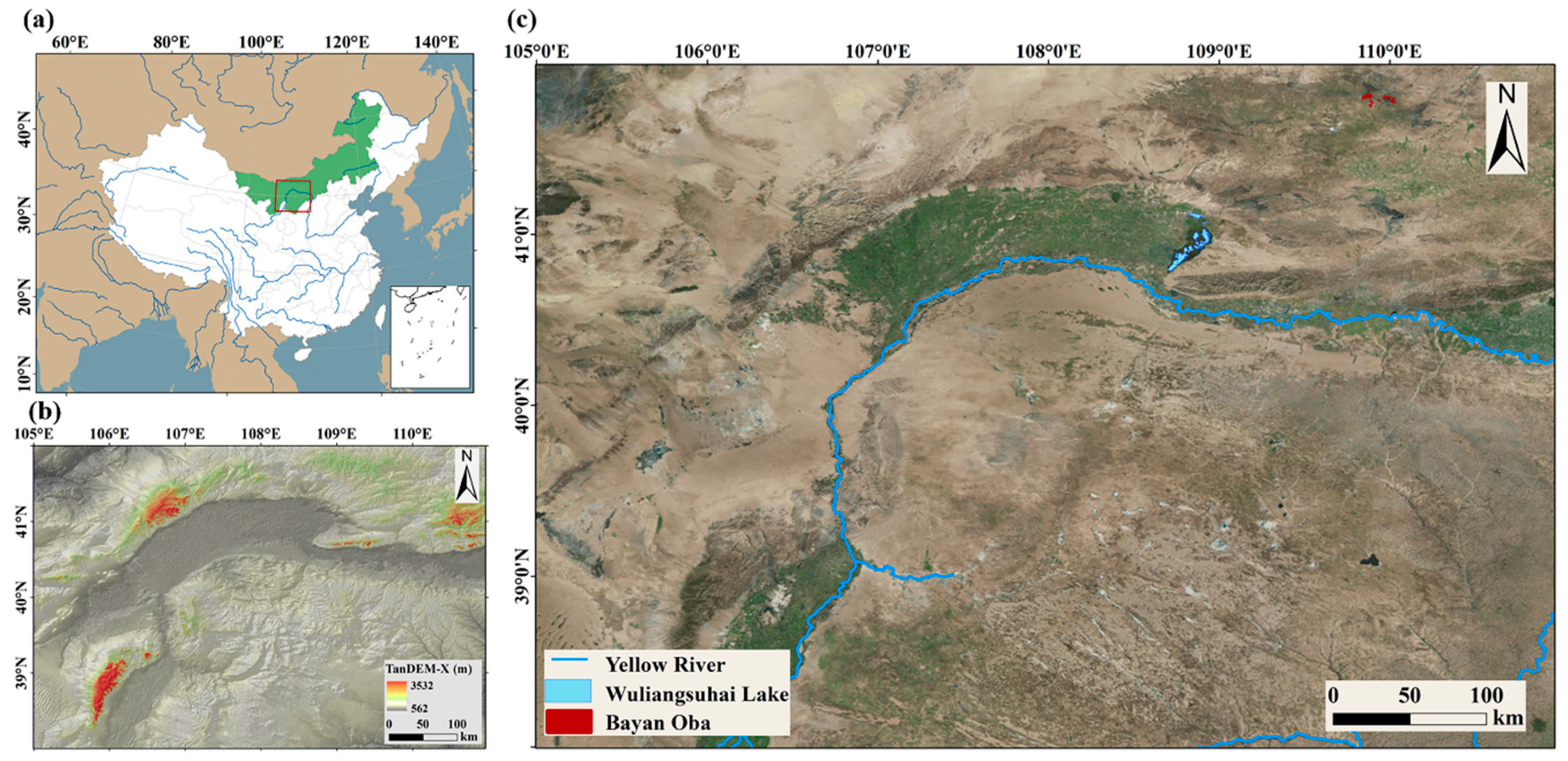
The study area is located in the southwest part of the Inner Mongolia Autonomous Region and a small proportion of the northern part of the Ningxia Hui Autonomous Region in northern China (38°00′N to 42°00′N, 105°00′E to 111°00′E), as shown in Figure 1. Eight cities are found in the study area, namely, Baotou, Bayan Nur, Ordos, Wuhai, Shizuishan, Yinchuan, Yulin, and Alxa League. It covers an area of approximately 227,500 km2 with altitudes ranging from 562 m to 3532 m. The climate of this region belongs to the temperate monsoon regime featured by few and irregular rainfalls, annual precipitation of 100–500 mm, and strong solar radiation. The temperature is around 25 °C in summer, and the lowest temperature is below −20 °C in winter. The vegetation cover mainly consists of trees, shrubs, subshrubs, and herbs [34,35]. This region is the flow area of the Yellow River, the second-longest river in China, and the Ulan Moron River. Wuliangsuhai Lake, one of the eight largest freshwater lakes in China, is also located in the study area. Dense open-pit mining areas are distributed in the study area, including Bayan Obo Mining Area, the world’s largest rare earth mine.
2.2. Data
2.2.1. Multitemporal DEM Data for Delineating Topographic Changes
Multitemporal DEMs were used to reveal the topographic changes due to mining activities. The Shuttle Radar Topography Mission Global Coverage DEM at 3” (~90 m) resolution (SRTM3), which measured land elevations by using space-borne radar measurements in February 2000, was utilized to represent the original topographic condition before the mining activities [36]. To contrast the topography after mining during the study period, we used the TanDEM-X DEM at 90 m resolution, which was acquired during the period from December 2010 to January 2015 by using space-borne synthetic aperture radar operating at X-band (accessed at https://geoservice.dlr.de/web/dataguide/tdm90/#access). The detailed description of the TanDEM-X mission and global DEM generation can be referred to in Rizzoli et al. [37].
2.2.2. Landsat Imagery for Delineating Land Surface Spectral Changes
The U.S. Geological Survey (USGS) provides Landsat 8 Collection 1 Tier 1 and real-time data calibrated top-of-atmosphere (TOA) reflectance raw scenes with the highest available data quality placed into Tier 1. The Tier 1 database includes Level-1 Precision and Terrain (L1TP) corrected data that have well-characterized radiometry and are intercalibrated across the different Landsat instruments. In this study, the selected imagery data was composed of four channels (red, green, blue, and near-infrared [NIR]) at 30 m resolution taken by USGS downloaded from the Google Earth Engine (GEE) website [38]. In the GEE website, 22 satellite imagery tiles between June and November from 2017 to 2018, with cloud cover features less than 0.1% were selected. These channels are used to calculate the normalized difference vegetation index (NDVI) [39], the index employed to detect surface vegetation changes, as well as the normalized difference water index (NDWI) [40], which is used to monitor changes related to water content in water bodies.
2.3. Methods
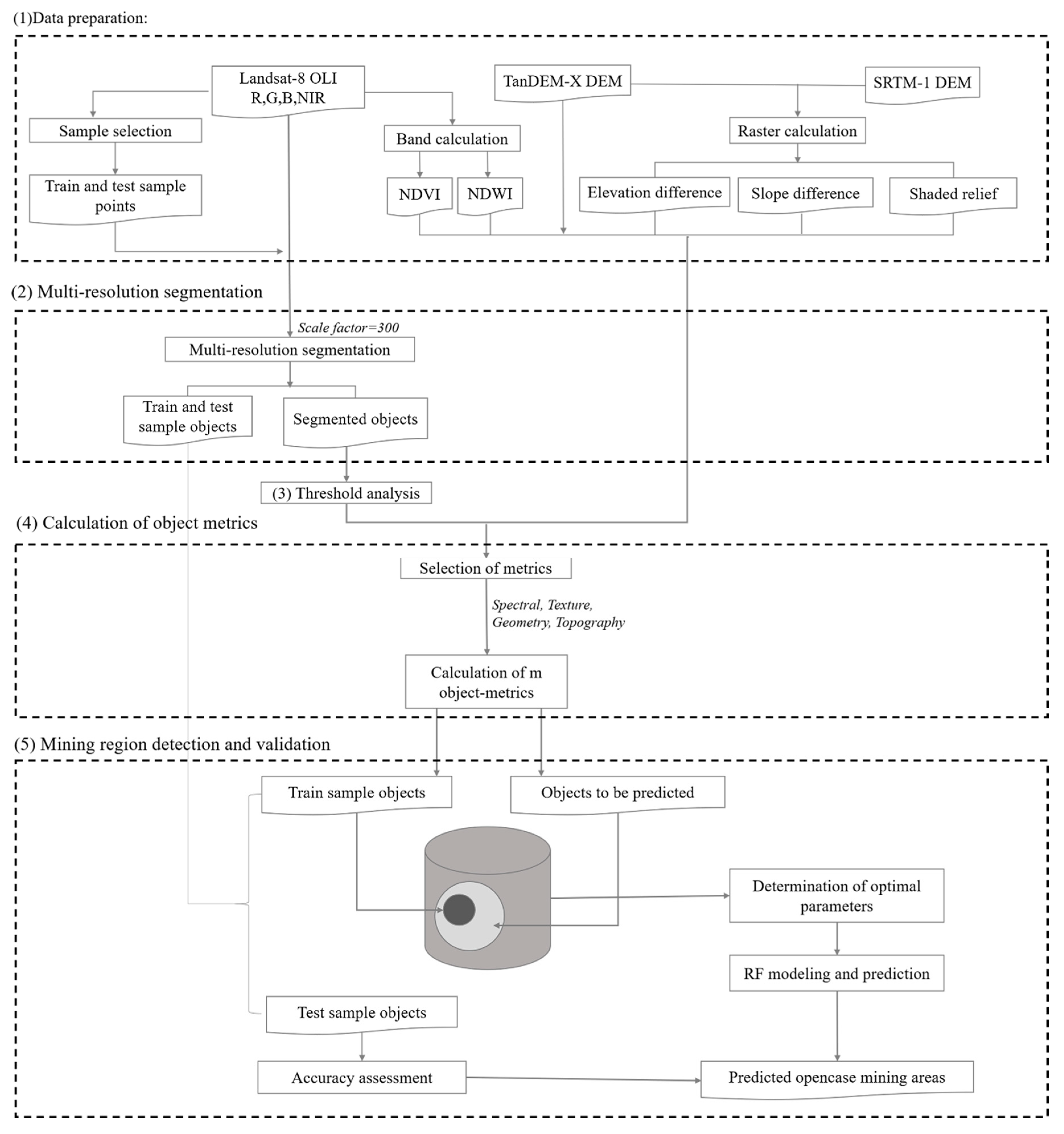
The proposed method includes five main steps, as illustrated in Figure 2: (1) data preparation with Landsat data and DEMs before and after mining activities, including the calculation of NDVI [39], NDWI [40], elevation difference, slope difference, and terrain relief, as well as the selection of train and test sample points (2) image segmentation using multiresolution segmentation methods [41], (3) threshold analysis to reduce the obvious non-mining area objects, (4) object metrics selection and calculation, and (5) RF modeling and prediction through the random Forest package in RStudio [42], and accuracy assessment. Details are given in the following sections.
2.3.1. Data Preparation
To enhance the contrasting information between the original and post-mining land surface and to improve the detection accuracy, aside from the raw spectral bands of the selected Landsat images and two epochs of DEM data (SRTM3 and TanDEM-X DEMs), a set of secondary variables from optical and topographic data was generated, including the NDVI and NDWI images, the elevation and slope difference maps, and a shaded relief map after mining activity. NDVI, which is an indicator employed for assessing live green vegetation, and NDWI, which is employed to monitor water content change in water bodies, were computed according to Equations (1) and (2) below [39,40]).
Hundreds of sample points were randomly selected and evenly distributed based on high-resolution imagery to generate train and test samples of mines and non-mines on Google Earth and the GIS software for further RF modeling. These sample points were then transferred to sample objects with a variety of features in eCognition. The number of test samples is about one-fifth that of the training set (test samples: train samples = 52:253).
2.3.2. Spectral Image Segmentation
Unlike pixel-based classification, OBIA uses both spectral and spatial information for classification based on information from a set of similar pixels called objects, while pixel-based classification is based solely on the spectral information in each pixel and mostly ignores the spatial context [43]. The use of OBIA to segment objects is effective in obtaining the extent of mining areas much more accurately than the pixel-based approach does, because some pixel values vary from different parts of a mining area, such as excavation and accumulation areas, making the delineation of the mines’ extents challenging.
Image segmentation is an important processing step of object-based image classification. Compared with other segmentation methods, MRIS implemented in eCognition software is evaluated well and has been widely used in many prior Earth science studies [41,44]. MRIS, a bottom-up segmentation algorithm that is also called the region growing algorithm, which starts from a single pixel and gradually merges larger objects according to the homogeneity criterion until the segmentation parameter is satisfied [45,46,47]. The criterion is composed by the scale parameter controlling the size of the merged regions (the process terminates when the smallest increase in homogeneity exceeds a user-defined threshold), the shape of segments, the influence of color (equal to 1 minus the shape of the segments), the weight of the compactness, and the smoothness of objects (equal to 1 minus the weight of the compactness) [48,49,50].
The four spectral bands—red, green, blue, and NIR—were used to segment the imagery covering the entire study area into multiple small objects by weighting with the same value. Multilevel segmented data with different scale parameters of 150, 300, and 450 were further used for RF classification on the basis of their shape and compactness (before determining the three factors with optimized results, we tested a wider range of different scale parameters). The scale parameters were chosen through trial and error to visually judge whether the segmented objects are too large or fracture (i.e., the object extent that is drawn is considerably outside the real extent, or many objects are found in one target area) so that the segmented object scale can be as optimum as possible in the target area. By default, the shape and compactness parameters were weighted with 0.1 and 0.5, respectively. We also tested other setting schemes for the two parameters, and the results have no obvious differences in detecting the targets. DEM and other data were not involved in the segmentation step as other variables (e.g., topographic factor based on DEM) are not featured with spectral-based segmentation (e.g., Red, Green, Blue).
2.3.3. Threshold Analysis
To decrease the time consumption of the segmentation as well as the calculation of characteristics and to effectively reduce misclassification, loose threshold ranges of the elevation and slope difference for potential mining target areas were set to mask out the absolutely non-mineral areas.
To explain the process of threshold analysis in an understandable way, the study area could be conceptually separated into three parts—mining areas, non-mining areas but similar to the mining areas in the spectral and topographic characteristics (non-mining areas I), and non-mining areas that could be identified easily (non-mining areas II). For the purpose of achieving the approximate region that must include whole mining areas and a small part of non-mining areas (i.e., non-mining areas I), the region where exact non-mineral areas exist (non-mining areas II) should be identified first (i.e., the whole study area minus the non-mining areas II to obtain the non-mining areas I and mining areas). Hence, a comparison of the elevation and slope difference between the mine and non-mine indicates that some certain ranges are applicable for both mines and non-mines. Therefore, to obtain the absolute non-mining areas, the threshold range should be set smaller than that of the real non-mining existing areas. For this study, for non-mining areas II, the range of elevation difference was roughly set from −0.5 m to 1 m and that of the slope difference was from 0° to 0.5°, the range to exclude water bodies and mountain areas. These ranges were set in eCognition and applied to all objects obtained from the segmentation process. These masked objects will not participate in the further object metrics calculation and RF classification. Consequently, the excluded area is about 92,000 km2, accounting for 40% of the entire study area.
2.3.4. Calculation of Object Metrics
According to previous studies, an overview of the features (Table 1) introduced a number of object metrics for all segments and will be applied for RF mining area prediction. Spectral features recommended in Nichol and Wong [51] applied in landslides include mean band values (red, green, blue, NIR, NDVI, and NDWI), mean brightness [50], and maximum difference index ( [52]. Both mines and landslides lead to the removal of land cover (e.g., vegetation) and exposure of underground materials (e.g., soil, rock). The mean brightness is defined as the sum of each object mean values in visible bands ( divided by the number of corresponding visible bands ( using the equation as follows:
The same visible bands were used to calculate for each object, which is defined as the absolute value of the difference of the maximum object mean ( and the minimum object mean divided by the mean brightness [52,53]:
In this study, the difference between mining regions and non-mining regions is reflected not only in the spectrum but also in the texture. Thus, a variety of derivatives of the gray-level co-occurrence matrix (GLCM) [53,54,55] derived by image object pixels and the mean value of all the layers has been adopted. Eight texture features of GLCM measures were selected: homogeneity, dissimilarity, entropy, correlation, contrast, angular second moment, mean, and standard deviation. These features were computed by using eCognition after segmentation.
The geometric information involving shape index, length–width, roundness, asymmetry, compactness, area, length, and the rectangular fit was also used for further classification. Apart from that, topographic properties (elevation difference, slope difference, DEM after mining activity, and terrain relief described in Section 3.1) were highly correlated with surface morphological changes and have good sensitivity to mine identification.
Although a total of 60 parameters, including spectral information, texture information, geometric information, and topographic information, were chosen, only some of them were used in the classification and were identified by using the RF cross-validation (RFCV), and variable importance (VI) functions based on the random Forest package. These two functions filter the most important parameters, rank them, and provide the most appropriate number of parameters. Therefore, parameters that are best suited for classification will be provided and involved in RF modeling and prediction.
2.3.5. Mining Region Detection and Validation
RF is an ensemble learning method for classification and regression proposed by Breiman [42]. This algorithm uses a bootstrap resampling method to extract a subset of training samples (referred to as in-bag samples) for decision tree modeling and then combines these decision trees to obtain the final predicted classification results [42]. Two key parameters in the RF classifier need to be set in advance: the number of decision trees (Ntree) and the number of variables set for the best split (Mtry). For classification accuracy, the Mtry parameter, is much more sensitive than the Ntree parameter. A prior study [56,57] empirically suggested that the Ntree parameter can be as large as possible because RF has high computational efficiency, although the error will tend to stabilize when it reaches 500. Theoretically, the Mtry parameter is usually set to the square root of the number of input variables [58]. Therefore, in this study, the Mtry parameter was set as 7, and the Ntree was set as 2000 by the random Forest package [59] in the R environment.
Feature selection, the most influential factor in the RF algorithm, can be determined by VI and the number of variables. For VI, the extract variable importance measure function was used in the random Forest package. At present, different ways can be used to measure VI, such as the mean decrease in accuracy (MDA) and the mean decrease in Gini (MDG) [42]. Many previous studies tend to use MDA to obtain VI [60]. The number of variables in the feature selection was calculated by the RFCV [61] function showing the cross-validated prediction performance of the models with a sequentially reduced number of predictors (ranked by variable importance) via a nested cross-validation procedure in the random Forest package. In this study, two groups of features were measured by VI and RFCV on the basis of the DEM data combined with spectral information and the spectral data only to compare the detection results of opencast mining regions. For the former multi-band image combination, the most accurate parameters are set as 13 variables (Combination I) in Table 2, while 25 variables were determined by the same method for the latter combination (Combination II). More features are speculated to be needed to participate in the classification without integrating DEMs to achieve high accuracy. Combinations I and II represent a certain number (13, 25) of variables for the DEM data combined with spectral information and the spectral data only, respectively. Out-of-bag (OOB) error is a method of measuring the prediction error of random forest to sub-sample data samples used for training. The OOB error rates of Combination I and Combination II are 7.54% and 12.70%, respectively. The detection accuracies for different combination methods to identify whether the object is the mining area or not were also validated by overlapping the test objects and predicted mapping mining regions and will be further analyzed in Section 3.1. Five accuracy measures are used: precision, recall, overall accuracy, the kappa coefficient, and the F-measure, which is able to measure classification performance-independent class imbalance [62]. The test samples for the mining area and non-mining area are about one-fifth of the training samples, that is, 32 and 20, respectively.
3. Results
3.1. Assessment of the Detection Result of Opencast Mining Regions
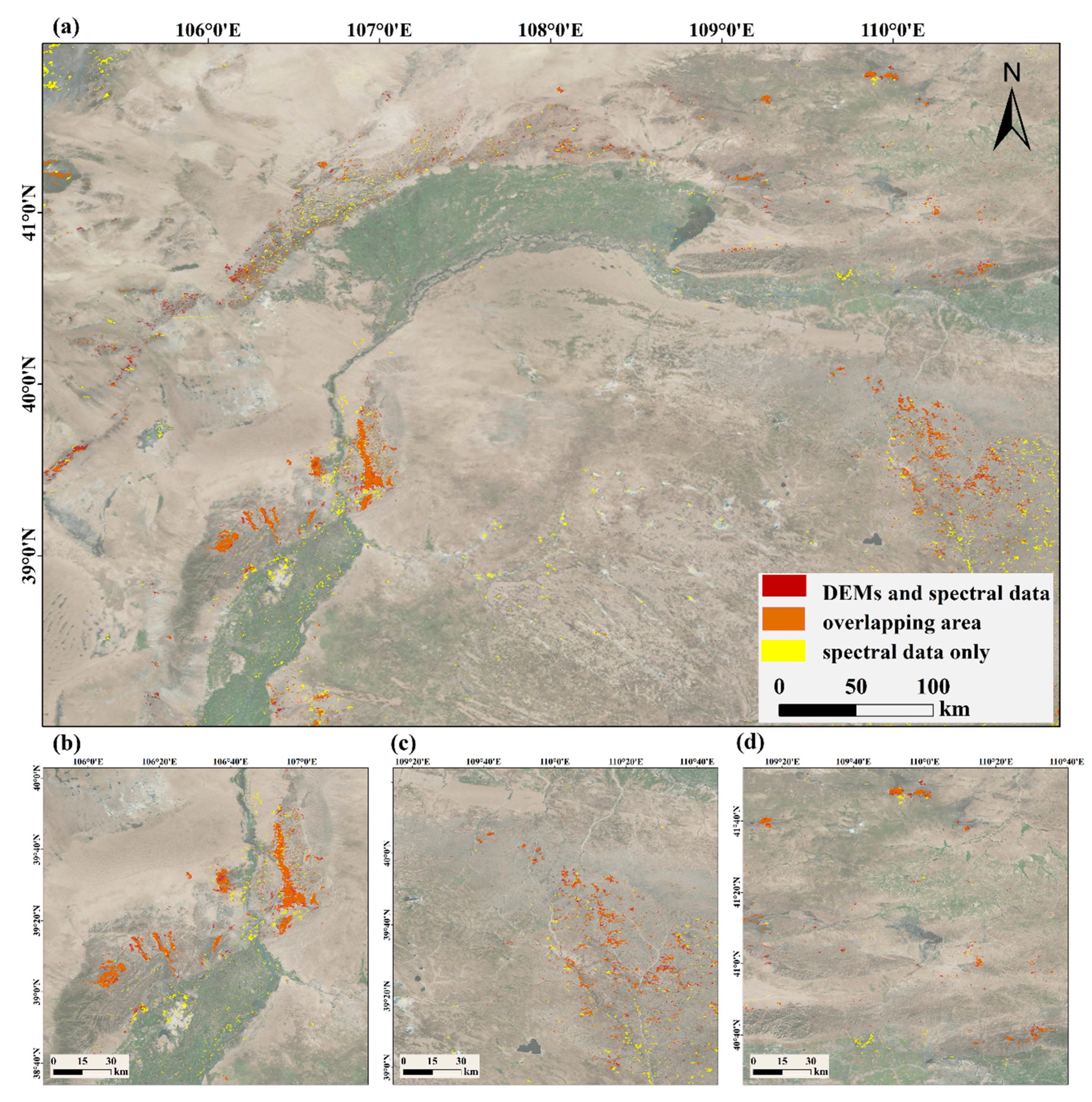
To indicate the effectiveness of the DEM data combined with other remote sensing measurements, the comparison of the predicted mining region results based on two different combination methods—spectral information only and the integration of DEM data and spectral information—was conducted in this study. For the scheme that uses DEM data combined with spectral information with 13 variables (i.e., Combination I), the classification result of mining areas is labeled in red and orange colors in Figure 3. In comparison, the yellow and orange colors show the identification result of the scheme that used only spectral data with 25 certain variables (i.e., Combination II). The orange-filled extents represent the overlapping mining areas detected by both Combinations I and II.
Without DEM-derived information (Figure 3a), a large number of sparsely distributed falsely identified targets exist in the classification results, which are mainly concentrated in the northwest, southeast, and central parts of the study region, as validated by high-resolution Google Earth imagery. In addition, the areas where the opencast mines are concentrated, especially in the southwest (Figure 3b) and the southeast area (Figure 3c), tend to have more misclassified spots. These misclassified regions are mainly concentrated in mountainous areas with shady slopes and rugged topographical relief as well as water bodies, such as lakes and river wetland because their spectral signals are similar to that of the mining area to some extent. However, significant improvements can be observed when DEM information in the form of elevation difference, slope difference, and terrain relief model was integrated into the step of object metrics calculation.
The area of mining fields identified by using spectral data (about 1300 km2, 9696 objects) is obviously larger than that derived from the combination of spectral data with DEMs (about 1100 km2, 8093 objects), while the mean area (0.1358 km2) of the mining objects without DEM parameters involved in the classification is slightly smaller than that with DEM participation (0.1394 km2). The object sizes for some surface features (e.g., shady slopes and rugged terrain) are relatively small due to the MRIS rules. Consequently, mining objects without the participation of DEM information are more fragmented, mainly because many misclassified piecemeal spots exist.
The fact that the accuracy measures of Combination I are all higher than that of Combination II (Table 3) indicates that the method of integrating DEM data and spectral imagery (i.e., adding both the topographic and spectral information in the classification) outperforms the method that used spectral data only.
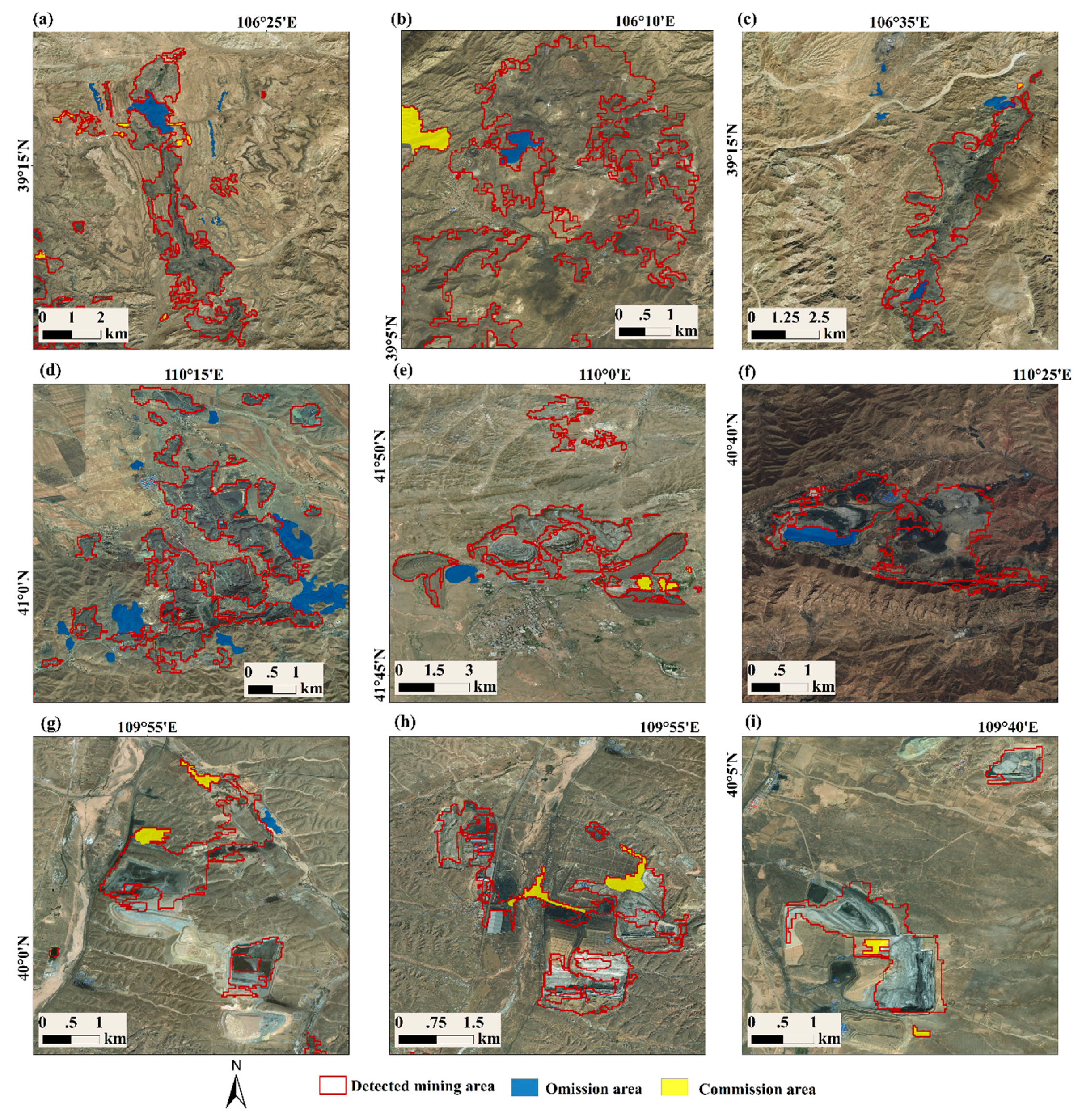
To assess the accuracy of the result of RF classification with metrics obtained from spectral and DEM data on a finer scale, we randomly selected nine sub-areas to locally observe the superposition of the classified objects of mining pits and mining areas boundaries, as well as the omission and commission areas (Figure 4). Note that the high-resolution background is not the imagery that was used in the segmentation. Therefore, the mapped mine objects do not exactly coincide with the spatial extent. The boundary of mapping opencast mines can reach about 90% of the actual boundary because the mining areas and the surrounding surface features (e.g., vegetation) perform differently in the spectrum. Thus, the mining area is likely to be distinguished from the other ground objects during segmentation according to the MRIS rules. Figure 4a–c shows places southwest of the study area, Figure 4d–e shows locations in the northeastern part, and Figure 4f–i presents locations in the southeastern part. An inevitable but not commonly seen phenomenon is that built-up areas with variable surface heights and the mountain terrains where the landslide occurred may pose negative influences on the classification result and were identified as commission areas. However, the classification result derived from the combination of the MRIS and RF algorithm can obviously capture well the shape of mining areas and produce relatively accurate locations of mining areas, including accumulation areas and excavation areas. Some tiny mining areas and the edge of large mining fields with relatively inapparent topographical changes are the main forms of omission areas. This study aims to detect the mining areas rather than map each pixel of the mines because this approach accepts a few differences in the boundaries between the real mines and the detected mines.
3.2. Spatial Characteristics of Opencast Mining Areas in the Study Area
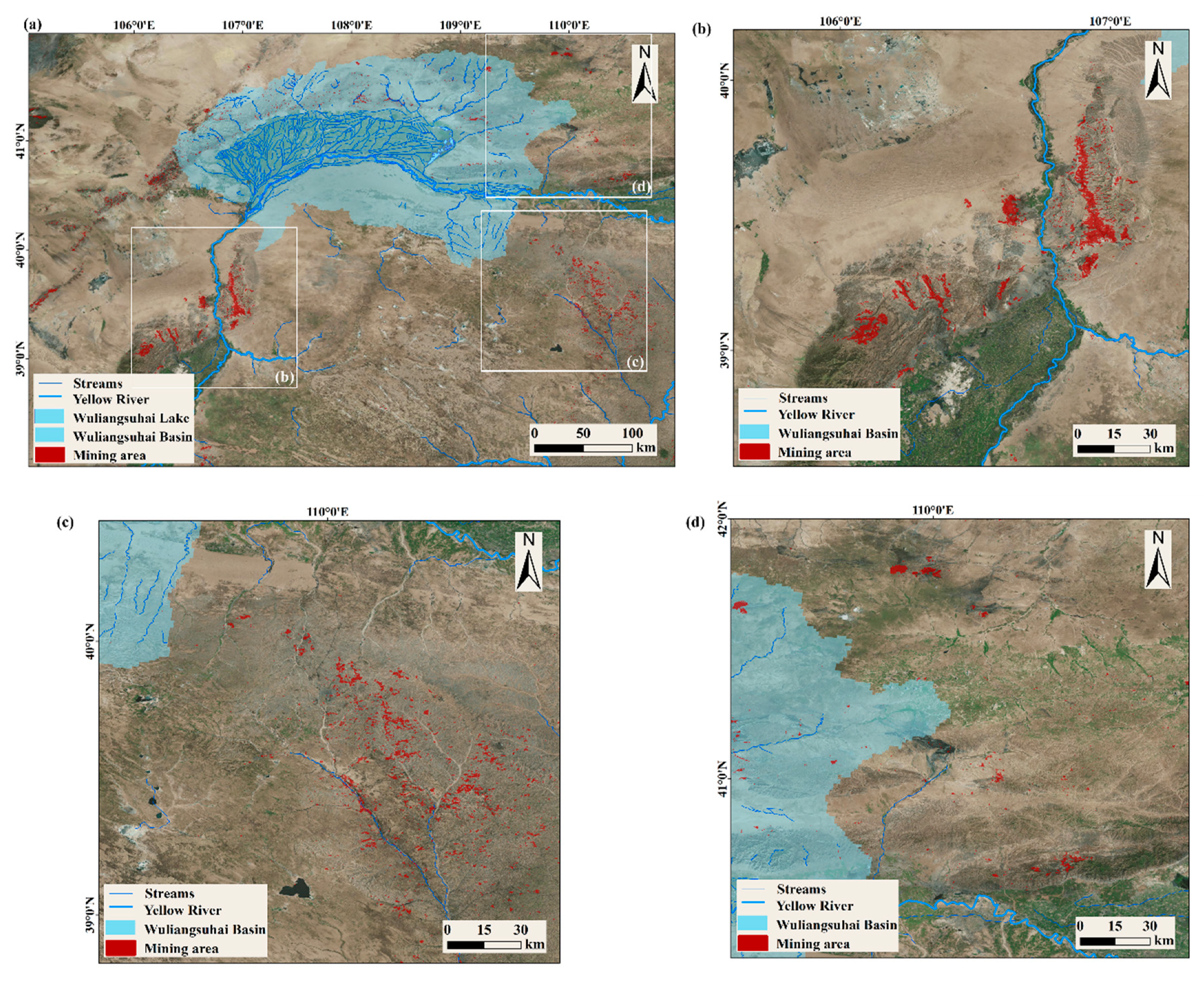
The distribution of the mining area tested by different parameters combination is shown in Figure 5a. In the southwestern part near Wuhai (Figure 5b), several large strip-shaped mining areas are found. A large number of small but densely distributed mining spots are also found in the southeast corner, between Yulin and Ordos (as shown in Figure 5c). In addition, several mining regions are scattered throughout the northeast or near Baotou (Figure 5d), including the world’s largest rare earth mine, Bayan Obo. Notably, many open-pit mining areas are close to the mainstream of the Yellow River, the second-longest river in China, and the upstream region of the Wuliangsuhai Lake basin, which is the main source of domestic freshwater for residents and irrigation water for vegetation and crops. Thus, the slag produced by mining could have an extremely negative impact on the water quality through surface runoff and groundwater flow and lead to surrounding ecological environment pollution.
3.3. Topographic Changes in Opencast Mining Areas
To reveal the influences of open-mining activities on geomorphologic landform in the study area, we compared the topographic features of the study area between pre-mining and post-mining periods on the basis of two different DEMs. The SRTM3 DEM acquired in February 2000 represents the surface morphology before mining activities. Some blank areas indicate missing SRTM data but have no effect on analyses results. By contrast, the terrain information provided by TanDEM-X DEM around 2012 indicates that the mining activities had substantially changed the local topography. The lowest post-mining elevation value is much lower than the lowest pre-mining value from 702 m to 562 m. Figure 6 reveals the explicit spatial changes in surface elevation after the detected mining activities to verify whether the elevation drops are due to the mining activities. The elevation change for each pixel in three local areas with dense mining areas was derived from the difference between SRTM3 DEM and TanDEM-X DEM. The deepest elevation dropped down to −258 m, and the highest rose to 162 m in the whole study area; both values were observed in the southwest of the study area (Figure 6b). The mean elevation was −0.9362 m due to the offset of excavation and accumulation areas. The classified area of open-pit mines was about 1,100 km2.
4. Discussion
4.1. Analysis of the Selection of the Classified Sample Points
The location and number of sample points that were chosen uniformly and randomly distributed in space and transferred to sample segmentation objects in eCognition directly determine the quality of the RF modeling result. The model was built through learning various object metrics of mining and non-mining sample objects and then lead to different classification results. Four sample combinations (i.e., Samples I, II, III, and VI) with different numbers and distribution overlapping with the Landsat imagery are shown in Figure 7. The numbers of mining points and non-mining points, as well as the OOB errors and the mean prediction error on each training sample, are shown in Table 4.
The rules for selecting these sample points took into account the sample location, the proportion, and the number of mining and non-mining samples. To be more specific, the difference between Samples I and II has almost the same proportional increase in both mining samples and non-mining samples, while the difference between Samples II and III is the increase only in non-mining areas. The similarity between Samples I and IV is the same proportion of mining and non-mining points, and the difference was the number of total points. To compare Samples I and II with Sample III, the total sample points were set as 72,213 and 253, respectively, and the resultant OOB errors were 11.11%, 9.91%, and 9.52%, respectively (Table 4). This finding means that the accuracy of RF prediction increases with the increase in the number of sample points. However, compared with that of Sample II, the sample point number in Sample IV (239) is larger, but the OOB error of Sample II is unexpectedly lower than that of Sample IV (Table 4). Their difference lies in the different proportions of samples for various classifiers. Therefore, the number of sample points could not be the only factor that determines the accuracy of the prediction result; the proportion of mining and non-mining sample points may also have an obvious impact on the classification [52]. Apart from the number and proportion of training points, the locations of those points also play an unignorable role. In this study, as the number of sample points increases, the training points of non-mining areas are mainly located in those areas with complex terrain, constantly changing elevation, and large topographic relief, such as mountainous areas, lakes, riverbanks, and desert area, which would expand the negative sample (i.e., non-mining samples) set and help correctly classify these terrains as non-mining areas. Consequently, Sample III was chosen eventually to produce the analyzed results due to the relatively low OOB error rate. A detail that is worth mentioning is that the RF algorithm focuses only on the data of each sample object metric for each segment, that is, the geographic coordination of training set objects will not be considered and do not have an influence on the further classification. Hence, even if a number of mining areas are set as sample points in Sample III, doing so will not affect the prediction step for the whole study region. Even the sample points were chosen as optimum as possible. Future work will focus on adjusting the distribution, proportion, and the number of sample points in the training set to further improve the accuracy of the open-pit mining detection results.
4.2. Variable Selection according to the Importance Ranking
A certain number of top-ranked object metrics was used in the RF algorithm to improve the mining pit recognition accuracy. The functions of RFCV and VI were used to rank the top 13 features from the 10-fold replicate runs on the basis of the random Forest package. These functions are listed in Table 2 to establish the RF model. In this study, from the result of RFCV and VI, the conclusion was that factors that are mostly related to topography and spectrum have relatively significant impact on RF classification, while texture information is important only in standard deviation. All terrain-related factors were chosen, including TanDEM-X, terrain relief, elevation difference, and slope difference. Six out of eight spectral information also ranked high. This finding suggests that topographic information plays a vital role in such a machine learning classification method, and texture-related and geometric features can be less focused on due to the high time-cost in the large-scale object metrics calculation. The difference between the top 13 variables and the 60 variables shown in Table 1 is that the identification accuracy is improved in reducing the error of omission and commission, and the overall accuracies for 13 variables and all 60 variables are 0.9423 and 0.9231, respectively.
4.3. Analysis of the Influences of Segmentation Scale Parameter on Detection Accuracy
The scale parameter plays a significant role in further RF modeling and open-pit mine prediction. That is, if the scale parameter was set too large, the MRIS algorithm might combine mining and non-mining areas as one object, which will result in the mine being wrongly identified as non-mine when the object value is less than the mean value, or vice versa. Conversely, if it is too small, then one mining region would be separated into multiple objects, and geometric information such that the area would be too small to be identified. In this study, the 13 variables calculated by RFCV and VI coincidentally excluded all the geometric information. Hence, the merge operation was performed, which might have caused the loss of tiny scattered objects and was not applicable to newly developed mining fields. However, no absolutely accurate standard is typically available to define the most appropriate scale parameter, although the Estimation of Scale Parameters tool for a single band (ESP tool) [48] and for multiband images (ESP2 tool) [63] are widely used in choosing a relatively optimum scale factor of the MRIS. In this study, the ESP2 tool was not suggested for use in such a large area because it requires multiple iterations and requires long processing time. RF is adapted for large datasets and can be used to calculate intrinsic measures of the variable through the calculation of permuting the value in the OOB sample and measuring the difference of the OOB errors before and after the permutation [64]. Those measures allow us to know which segmentation scale is more recommended for identifying a particular geographic object [65].
In this study, we compared three different segmentation scales at 150, 300, and 450, respectively. The corresponding total objects at different scales were 27.62 × 10⁵, 6.92 × 10⁵, and 2.99 × 10⁵, and their OOB errors wre 9.52%, 9.52%, and 9.64%, respectively. Considering the computing effectiveness for the large area, for example, the number of generated objects with a segmentation scale of 150 is about four times larger than that at the scale of 300, and the OOB errors for the scales of 150 and 300 are nearly the same, the relatively appropriate scale parameter was recommended to be about 300 in this study. The detection result may inevitably deviate from mine distribution in the real world because of the temporal offset of DEM data and high-resolution images.
5. Conclusions
Mineral resources are a necessary support for human activities. With the increasingly frequent mining activities in the world, open-pit mining has an impact on LULC, and poses a serious threat to downstream settlements, and the environment. Therefore, being able to identify the location, extent, and period of mining activities by using a robust and efficient algorithm is of critical importance to investigate mining areas and illegal mining activities. In this study, by integrating DEMs (TanDEM-X and SRTM3) and Landsat spectral data, we used image segmentation and object-based image analysis to divide a large area into tens of thousands of small objects on the basis of their spectral features. Through the innovation of combining spectral and topographic change information, 60 spectral, topographic, and textural features of each object were obtained for classification by using the RF algorithm. Our results suggest that the RF algorithm can effectively detect the attribute characteristics of opencast mining samples through integrating spectral imagery and multitemporal DEMs at a large scale. This finding was derived from our test result on open-mining development in the mineral-rich inner Mongolia area. The identified mining area is about 1,100 km2, with an elevation change ranging from −258 m to 162 m in this study area and period.
A comparison between the identified mine boundary and the actual mine boundary, as validated by high-resolution images, shows that the proposed method can well capture the location and delineate the boundary of the mining fields. The detection results obtained by integrating spectral signal and topographical change information can obviously outperform some mapping methods based on optical images only, 94.23%, in comparison with 90.38% in the overall accuracy. An analysis of the classified samples indicates that the number of training samples and the proportion of targeted mining and non-mining areas could obviously affect the OOB accuracy. In future research, we will further optimize the method and inventory of opencast mining areas worldwide.
Author Contributions
Conceptualization, C.S. and K.L.; Data curation, Q.W.; Funding acquisition, C.S.; Methodology, Q.W., C.S., K.L. and L.K.; Project administration, C.S.; Software, Q.W.; Supervision, C.S., K.L. and L.K.; Validation, Q.W.; Visualization, Q.W.; Writing—original draft, Q.W. and C.S.; Writing—review & editing, C.S., K.L. and L.K. All authors have read and agreed to the published version of the manuscript.
Funding
This work was partly funded by the Strategic Priority Research Program of the Chinese Academy of Sciences (Grant No. XDA23100102), the Thousand Young Talents Program in China (Grant No. Y7QR011001), the National Key Research and Development Program of China (Grant No. 2019YFA0607101, 2018YFD1100101), and the National Natural Science Foundation of China (No. 41971403, 41801321).
Acknowledgments
We are grateful for the U.S. Geological Survey’s Earth Resources Observation and Science (EROS) Center and the Earth Observation Center of the German Aerospace Center for providing Landsat imagery, SRTM DEM and TanDEM-X DEM data.
Conflicts of Interest
The authors declare no conflict of interest.
References
- Otukei, J.R.; Blaschke, T. Land cover change assessment using decision trees, support vector machines and maximum likelihood classification algorithms. Int. J. Appl. Earth Obs. Geoinf. 2010, 12, S27–S31. [Google Scholar] [CrossRef]
- Petropoulos, G.P.; Partsinevelos, P.; Mitraka, Z. Change detection of surface mining activity and reclamation based on a machine learning approach of multi-temporal Landsat TM imagery. Geocarto Int. 2013, 28, 323–342. [Google Scholar] [CrossRef]
- Styers, D.M.; Chappelka, A.H. Urbanization and atmospheric deposition: Use of bioindicators in determining patterns of land-use change in west Georgia. Water Air Soil Pollut. 2009, 200, 371–386. [Google Scholar] [CrossRef] [Green Version]
- Latifovic, R.; Fytas, K.; Chen, J.; Paraszczak, J. Assessing land cover change resulting from large surface mining development. Int. J. Appl. Earth Obs. Geoinf. 2005, 7, 29–48. [Google Scholar] [CrossRef]
- Moreno-de Las Heras, M.; Merino-Martín, L.; Nicolau, J.M. Effect of vegetation cover on the hydrology of reclaimed mining soils under Mediterranean-Continental climate. Catena 2009, 77, 39–47. [Google Scholar] [CrossRef]
- Gesch, D.B. Analysis of multi-temporal geospatial data sets to assess the landscape effects of surface mining. In Proceedings of the National Meeting of the American Society of Mining and Reclamation, Lexington, KY, USA, 19–23 June 2005; pp. 415–432. [Google Scholar]
- Carlson, T.N.; Ripley, D.A.; Schmugge, T.J. Rapid soil drying and its implications for remote sensing of soil moisture and the surface energy fluxes. In Thermal Remote Sensing in Land Surface Processing; CRC Press: Boca Raton, FL, USA, 2004; pp. 207–226. [Google Scholar]
- De Smedt, F.; Liu, Y.; Gebremeskel, S.; Hoffmann, L.; Pfister, L. Application of GIS and remote sensing in flood modelling for complex terrain. IAHS Publ. 2004, 289, 23–32. [Google Scholar]
- DeFries, R.; Eshleman, K.N. Land-use change and hydrologic processes: A major focus for the future. Hydrol. Process. 2004, 18, 2183–2186. [Google Scholar] [CrossRef]
- Finch, D.M. Habitat use and habitat overlap of riparian birds in three elevational zones: Ecological archives E070-001. Ecology 1989, 70, 866–880. [Google Scholar] [CrossRef]
- Foley, J.A.; Asner, G.P.; Costa, M.H.; Coe, M.T.; DeFries, R.; Gibbs, H.K.; Howard, E.A.; Olson, S.; Patz, J.; Ramankutty, N.; et al. Amazonia revealed: Forest degradation and loss of ecosystem goods and services in the Amazon Basin. Front. Ecol. Environ. 2007, 5, 25–32. [Google Scholar] [CrossRef]
- Foody, G.M.; Mathur, A. Toward intelligent training of supervised image classifications: Directing training data acquisition for SVM classification. Remote Sens. Environ. 2004, 93, 107–117. [Google Scholar] [CrossRef]
- Genxu, W.; Yibo, W.; Ju, Q.; Qingbo, W. Land cover change and its impacts on soil C and N in two watersheds in the center of the Qinghai-Tibetan Plateau. Mt. Res. Dev. 2006, 26, 153–163. [Google Scholar] [CrossRef]
- Griffith, J.A. Geographic techniques and recent applications of remote sensing to landscape-water quality studies. Water Air Soil Pollut. 2002, 138, 181–197. [Google Scholar] [CrossRef]
- Miller, J.D.; Yool, S.R. Mapping forest post-fire canopy consumption in several overstory types using multi-temporal Landsat TM and ETM data. Remote Sens. Environ. 2002, 82, 481–496. [Google Scholar] [CrossRef]
- Shuster, W.D.; Bonta, J.; Thurston, H.; Warnemuende, E.; Smith, D. Impacts of impervious surface on watershed hydrology: A review. Urban Water J. 2005, 2, 263–275. [Google Scholar] [CrossRef]
- Weng, Q. A remote sensing GIS evaluation of urban expansion and its impact on surface temperature in the Zhujiang Delta, China. Int. J. Remote Sens. 2001, 22, 1999–2014. [Google Scholar]
- Abuelgasim, A.; Chung, C.-j.; Champagne, C.; Staenz, K.; Monet, S.; Fung, K. Use of multi-temporal remotely sensed data for monitoring land reclamation in Sudbury, Ontario (Canada). In Proceedings of the 2005 International Workshop on the Analysis of Multi-Temporal Remote Sensing Images, Sydney, Australia, 31 May 2005; Institute of Electrical and Electronics Engineers: Sydney, Australia, 2005; pp. 229–235. [Google Scholar]
- Gillanders, S.N.; Coops, N.C.; Wulder, M.A.; Gergel, S.E.; Nelson, T. Multitemporal remote sensing of landscape dynamics and pattern change: Describing natural and anthropogenic trends. Prog. Phys. Geogr. 2008, 32, 503–528. [Google Scholar] [CrossRef]
- Ieronimidi, E.; Mertikas, S.P.; Hristopoulos, D. Fusion of Quickbird satellite images for vegetation monitoring in previously mined reclaimed areas. In Proceedings of the Remote Sensing for Environmental Monitoring, GIS Applications, and Geology VI, Stockholm, Sweden, 11–14 September 2006; International Society for Optics and Photonics: Bellingham, WA, USA, 2006; p. 636611. [Google Scholar]
- Pagot, E.; Pesaresi, M.; Buda, D.; Ehrlich, D. Development of an object-oriented classification model using very high resolution satellite imagery for monitoring diamond mining activity. Int. J. Remote Sens. 2008, 29, 499–512. [Google Scholar] [CrossRef]
- Demirel, N.; Emil, M.K.; Duzgun, H.S. Surface coal mine area monitoring using multi-temporal high-resolution satellite imagery. Int. J. Coal Geol. 2011, 86, 3–11. [Google Scholar] [CrossRef]
- Li, J.; Zipper, C.E.; Donovan, P.F.; Wynne, R.H.; Oliphant, A.J. Reconstructing disturbance history for an intensively mined region by time-series analysis of Landsat imagery. Environ. Monit. Assess. 2015, 187, 557. [Google Scholar] [CrossRef]
- Sen, S.; Zipper, C.E.; Wynne, R.H.; Donovan, P.F. Identifying revegetated mines as disturbance/recovery trajectories using an interannual Landsat chronosequence. Photogramm. Eng. Remote Sens. 2012, 78, 223–235. [Google Scholar] [CrossRef]
- Townsend, P.A.; Helmers, D.P.; Kingdon, C.C.; McNeil, B.E.; de Beurs, K.M.; Eshleman, K.N. Changes in the extent of surface mining and reclamation in the Central Appalachians detected using a 1976–2006 Landsat time series. Remote Sens. Environ. 2009, 113, 62–72. [Google Scholar] [CrossRef]
- Homer, C.H.; Fry, J.A.; Barnes, C.A. The national land cover database. US Geol. Surv. Fact Sheet. 2012, 3020, 1–4. [Google Scholar]
- Price, S.J.; Dorcas, M.E.; Gallant, A.L.; Klaver, R.W.; Willson, J.D. Three decades of urbanization: Estimating the impact of land-cover change on stream salamander populations. Biol. Conserv. 2006, 133, 436–441. [Google Scholar] [CrossRef]
- Hayakawa, Y.S.; Oguchi, T.; Lin, Z. Comparison of new and existing global digital elevation models: ASTER G-DEM and SRTM-3. Geophys. Res. Lett. 2008, 35, 17404. [Google Scholar] [CrossRef]
- Quinn, M.A.; Kepner, R.; Walgenbach, D.; Foster, R.N.; Bohls, R.; Pooler, P.; Reuter, K.; Swain, J. Effect of habitat characteristics and perturbation from insecticides on the community dynamics of ground beetles (Coleoptera: Carabidae) on mixed-grass rangeland. Environ. Entomol. 1991, 20, 1285–1294. [Google Scholar] [CrossRef]
- Srivastava, S.; Thakur, I.S. Evaluation of biosorption potency of Acinetobacter sp. for removal of hexavalent chromium from tannery effluent. Biodegradation 2007, 18, 637–646. [Google Scholar] [CrossRef]
- Gruber, A.; Wessel, B.; Huber, M.; Roth, A. Operational TanDEM-X DEM calibration and first validation results. ISPRS J. Photogramm. Remote Sens. 2012, 73, 39–49. [Google Scholar] [CrossRef]
- Gdulová, K.; Marešová, J.; Moudrý, V. Accuracy assessment of the global TanDEM-X digital elevation model in a mountain environment. Remote Sens. Environ. 2020, 241, 111724. [Google Scholar] [CrossRef]
- Wessel, B.; Huber, M.; Wohlfart, C.; Marschalk, U.; Kosmann, D.; Roth, A. Accuracy assessment of the global TanDEM-X Digital Elevation Model with GPS data. ISPRS J. Photogramm. Remote Sens. 2018, 139, 171–182. [Google Scholar] [CrossRef]
- Chen, X.; Wang, H. Spatial and temporal variations of vegetation belts and vegetation cover degrees in Inner Mongolia from 1982 to 2003. Acta Geogr. Sin. 2009, 64, 84–94. [Google Scholar]
- Chuai, X.W.; Huang, X.J.; Wang, W.J.; Bao, G. NDVI, temperature and precipitation changes and their relationships with different vegetation types during 1998-2007 in Inner Mongolia, China. Int. J. Climatol. 2013, 33, 1696–1706. [Google Scholar] [CrossRef]
- Farr, T.G.; Kobrick, M. Shuttle Radar Topography Mission produces a wealth of data. Eos Trans. Am. Geophys. Union 2000, 81, 583–585. [Google Scholar] [CrossRef]
- Rizzoli, P.; Martone, M.; Gonzalez, C.; Wecklich, C.; Tridon, D.B.; Bräutigam, B.; Bachmann, M.; Schulze, D.; Fritz, T.; Huber, M.; et al. Generation and performance assessment of the global TanDEM-X digital elevation model. ISPRS J. Photogramm. Remote Sens. 2017, 132, 119–139. [Google Scholar] [CrossRef] [Green Version]
- Gorelick, N.; Hancher, M.; Dixon, M.; Ilyushchenko, S.; Thau, D.; Moore, R. Google Earth Engine: Planetary scale geospatial analysis for everyone. Remote Sens. Environ. 2017, 202, 18–27. [Google Scholar] [CrossRef]
- Tucker, C.J.; Pinzon, J.E.; Brown, M.E.; Slayback, D.A.; Pak, E.W.; Mahoney, R.; Vermote, E.F.; El Saleous, N. An extended AVHRR 8-km NDVI dataset compatible with MODIS and SPOT vegetation NDVI data. Int. J. Remote Sens. 2005, 26, 4485–4498. [Google Scholar] [CrossRef]
- McFeeters, S.K. The use of the Normalized Difference Water Index (NDWI) in the delineation of open water features. Int. J. Remote Sens. 1996, 17, 1425–1432. [Google Scholar] [CrossRef]
- Blaschke, T. Object based image analysis for remote sensing. ISPRS J. Photogramm. Remote Sens. 2010, 65, 2–16. [Google Scholar] [CrossRef] [Green Version]
- Breiman, L. Random forests. Mach. Learn. 2001, 45, 5–32. [Google Scholar] [CrossRef] [Green Version]
- Hussain, M.; Chen, D.; Cheng, A.; Wei, H.; Stanley, D. Change detection from remotely sensed images: From pixel-based to object-based approaches. ISPRS J. Photogramm. Remote Sens. 2013, 80, 91–106. [Google Scholar] [CrossRef]
- Baatz, M.; Schäpe, A. Multiresolution segmentation—An optimization approach for high quality multi-scale image segmentation. In Angewandte Geographische Informations-Verarbeitung XII; Strobl, J., Blaschke, T., Griesebner, G., Eds.; Wichmann Verlag: Karlsruhe, Germany, 2000; pp. 12–23. [Google Scholar]
- Benz, U.C.; Hofmann, P.; Willhauck, G.; Lingenfelder, I.; Heynen, M. Multi-resolution, object-oriented fuzzy analysis of remote sensing data for GIS-ready information. ISPRS J. Photogramm. Remote Sens. 2004, 58, 239–258. [Google Scholar] [CrossRef]
- Ding, H.; Liu, K.; Chen, X.; Xiong, L.; Tang, G.; Qiu, F.; Strobl, J. Optimized Segmentation Based on the Weighted Aggregation Method for Loess Bank Gully Mapping. Remote Sens. 2020, 12, 793. [Google Scholar] [CrossRef] [Green Version]
- Liu, K.; Ding, H.; Tang, G.; Zhu, A.-X.; Yang, X.; Jiang, S.; Cao, J. An object-based approach for two-level gully feature mapping using high-resolution DEM and imagery: A case study on hilly loess plateau region, China. Chin. Geogr. Sci. 2017, 27, 415–430. [Google Scholar] [CrossRef]
- Drǎguţ, L.; Tiede, D.; Levick, S.R. ESP: A tool to estimate scale parameter for multiresolution image segmentation of remotely sensed data. Int. J. Geogr. Inf. Sci. 2010, 24, 859–871. [Google Scholar] [CrossRef]
- Espindola, G.; Câmara, G.; Reis, I.; Bins, L.; Monteiro, A. Parameter selection for region-growing image segmentation algorithms using spatial autocorrelation. Int. J. Remote Sens. 2006, 27, 3035–3040. [Google Scholar] [CrossRef]
- Martha, T.R.; Kerle, N.; Jetten, V.; van Westen, C.J.; Kumar, K.V. Characterising spectral, spatial and morphometric properties of landslides for semi-automatic detection using object-oriented methods. Geomorphology 2010, 116, 24–36. [Google Scholar] [CrossRef]
- Nichol, J.; Wong, M. Satellite remote sensing for detailed landslide inventories using change detection and image fusion. Int. J. Remote Sens. 2005, 26, 1913–1926. [Google Scholar] [CrossRef]
- Stumpf, A.; Kerle, N. Object-oriented mapping of landslides using Random Forests. Remote Sens. Environ. 2011, 115, 2564–2577. [Google Scholar] [CrossRef]
- Trimble. eCognition Developer Reference Book 9.0; Trimble: Munich, Germany, 2014. [Google Scholar]
- Haralick, R.M.; Shanmugam, K.; Dinstein, I.H. Textural features for image classification. IEEE Trans. Syst. Man Cybern. 1973, SMC-3, 610–621. [Google Scholar] [CrossRef] [Green Version]
- Marceau, D.J.; Howarth, P.J.; Dubois, J.-M.M.; Gratton, D.J. Evaluation of the grey-level co-occurrence matrix method for land-cover classification using SPOT imagery. IEEE Trans. Geosci. Remote Sens. 1990, 28, 513–519. [Google Scholar] [CrossRef]
- Belgiu, M.; Drăguţ, L. Random forest in remote sensing: A review of applications and future directions. ISPRS J. Photogramm. Remote Sens. 2016, 114, 24–31. [Google Scholar] [CrossRef]
- Guan, H.; Li, J.; Chapman, M.; Deng, F.; Ji, Z.; Yang, X. Integration of orthoimagery and lidar data for object-based urban thematic mapping using random forests. Int. J. Remote Sens. 2013, 34, 5166–5186. [Google Scholar] [CrossRef]
- Gislason, P.O.; Benediktsson, J.A.; Sveinsson, J.R. Random forests for land cover classification. Pattern Recognit. Lett. 2006, 27, 294–300. [Google Scholar] [CrossRef]
- Liaw, A.; Wiener, M. Classification and regression by randomForest. R News 2002, 2, 18–22. [Google Scholar]
- Schmidt, A.; Niemeyer, J.; Rottensteiner, F.; Soergel, U. Contextual classification of full waveform lidar data in the Wadden Sea. IEEE Geosci. Remote Sens. Lett. 2014, 11, 1614–1618. [Google Scholar] [CrossRef]
- Svetnik, V.; Liaw, A.; Tong, C.; Wang, T. Application of Breiman’s random forest to modeling structure-activity relationships of pharmaceutical molecules. In Proceedings of the Multiple Classifier Systems, International Workshop, MCS 2004, Cagliari, Italy, 9–11 June 2004; pp. 334–343. [Google Scholar]
- Bekkar, M.; Djemaa, H.K.; Alitouche, T.A. Evaluation measures for models assessment over imbalanced data sets. J. Inf. Eng. Appl. 2013, 3, 27–38. [Google Scholar]
- Drăguţ, L.; Csillik, O.; Eisank, C.; Tiede, D. Automated parameterisation for multi-scale image segmentation on multiple layers. ISPRS J. Photogramm. Remote Sens. 2014, 88, 119–127. [Google Scholar] [CrossRef] [Green Version]
- Puissant, A.; Rougier, S.; Stumpf, A. Object-oriented mapping of urban trees using Random Forest classifiers. Int. J. Appl. Earth Obs. Geoinf. 2014, 26, 235–245. [Google Scholar] [CrossRef]
- Duro, D.C.; Franklin, S.E.; Dubé, M.G. Multi-scale object-based image analysis and feature selection of multi-sensor earth observation imagery using random forests. Int. J. Remote Sens. 2012, 33, 4502–4526. [Google Scholar] [CrossRef]
Figure 1.
Study area in the southwestern Inner Mongolia Autonomous Region in northern China. (a) The location of the study area in southern Inner Mongolia Autonomous Region, China. (b) The study area in relation to the TanDEM-X scene. (c) The study area in true color image with the Yellow River, Wuliangsuhai Lake, and Bayan Obo Mining District.

Figure 2.
Workflow of the proposed method for detecting large-scale mining-ruined land by object-based image analysis (OBIA) and RF. The process includes data preparation, multiresolution image segmentation (MRIS), threshold analysis, object metrics calculation, and mine detection and validation.
Figure 2.
Workflow of the proposed method for detecting large-scale mining-ruined land by object-based image analysis (OBIA) and RF. The process includes data preparation, multiresolution image segmentation (MRIS), threshold analysis, object metrics calculation, and mine detection and validation.

Figure 3.
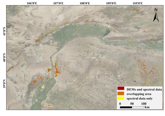
Comparison of mining area identification results on the basis of spectral data combined with Digital Elevation Model data and only spectral data. (a) the distribution of mining areas in the whole study area, (b) in the southwestern part, (c) in the southeast, and (d) in the northeast of the study area.
Figure 3.
Comparison of mining area identification results on the basis of spectral data combined with Digital Elevation Model data and only spectral data. (a) the distribution of mining areas in the whole study area, (b) in the southwestern part, (c) in the southeast, and (d) in the northeast of the study area.

Figure 4.
Superimposed map of real mining areas and identified geological areas with omission and commission areas. (a–c) are located in the southwest of the study area, (d,e) lie in the northeastern part, and (f–i) are situated in the southeastern part.
Figure 4.
Superimposed map of real mining areas and identified geological areas with omission and commission areas. (a–c) are located in the southwest of the study area, (d,e) lie in the northeastern part, and (f–i) are situated in the southeastern part.

Figure 5.
Distribution of mining areas segmented and classified by the MRIS and RF algorithm with streams, Yellow River, Wuliangsuhai Lake, and basin. (a) The distribution of mining areas and the distance to water bodies in the whole study area, (b) the southwestern part of the study area where the Yellow River goes through, (c) the southeast of the study area with streams, and (d) the northeast of the study area close to or in the Wuliangsuhai Basin.

Figure 6.
Elevation difference derived from the TanDEM-X and SRTM3. (a) the distribution of mining areas in the whole study area with elevation difference, (b) in the southwestern part, (c) in the southeast, and (d) in the northeast of the study area.
Figure 6.
Elevation difference derived from the TanDEM-X and SRTM3. (a) the distribution of mining areas in the whole study area with elevation difference, (b) in the southwestern part, (c) in the southeast, and (d) in the northeast of the study area.

Figure 7.
Distribution and number of sample points. (a) Sample I has only 72 sample points (mine points:non-mine points = 26:46), (b) Sample II has 213 sample points (mine points:non-mine points = 71:142, (c) Sample III has 253 sample points (mine points:non-mine points = 71:182, (d) Sample IV has 239 points (mine points:non-mine points = 85:154).


Table 1.
Overview of features used in mineral area detection.
| Feature Type | Feature Name | Acronym | Number |
|---|---|---|---|
| Spectral Information | Mean brightness | Brightness | 1 |
| Maximum difference index | Max_diff | 1 | |
| Mean band value | Red; Green; Blue; NIR; NDVI; NDWI; | 6 | |
| Texture information | GLCM homogeneity | All.dir; 0°;45°;90°;135° | 5 |
| GLCM dissimilarity | All.dir; 0°;45°;90°;135° | 5 | |
| GLCM entropy | All.dir; 0°;45°;90°;135° | 5 | |
| GLCM correlation | All.dir; 0°;45°;90°;135° | 5 | |
| GLCM contrast | All.dir; 0°;45°;90°;135° | 5 | |
| GLCM angular second moment | All.dir; 0°;45°;90°;135° | 5 | |
| GLCM mean | All.dir; 0°;45°;90°;135° | 5 | |
| GLCM standard deviation | All.dir; 0°;45°;90°;135° | 5 | |
| Geometric information | Shape index | Shape index | 1 |
| Length-width | Length-width | 1 | |
| Roundness | Roundness | 1 | |
| Asymmetry | Asymmetry | 1 | |
| Compactness | Compactness | 1 | |
| Area | Area | 1 | |
| Length | Length | 1 | |
| Rectangular fit | Rectangular fit | 1 | |
| Topographic information | Mean DEM | TanDEM-X | 1 |
| Mean elevation difference | Elevation difference | 1 | |
| Mean slope difference | Slope difference | 1 | |
| Mean terrain relief | Terrain relief | 1 |
Table 2.
Top 13 features ranked by Random Forest Cross-Validation and Variable Importance in RStudio.
Table 2.
Top 13 features ranked by Random Forest Cross-Validation and Variable Importance in RStudio.
| Feature Type | Feature Name | MDA |
|---|---|---|
| Spectral Information | Max_diff | 54.0082 |
| Topographic information | Terrain relief | 45.5290 |
| Topographic information | TanDEM-X | 38.3774 |
| Spectral Information | Blue | 31.7928 |
| Spectral Information | NIR | 29.8755 |
| Spectral Information | NDVI | 26.9931 |
| Spectral Information | NDWI | 26.6775 |
| Topographic information | Elevation difference | 26.2670 |
| Topographic information | Slope difference | 24.1456 |
| Spectral Information | Brightness | 22.8597 |
| Texture information | GCLM.StdDev.90° | 22.0214 |
| Texture information | GCLM.StdDev.all.dir | 19.2742 |
| Texture information | GCLM.StdDev.45° | 18.6994 |
Table 3.
Precision, recall, overall accuracy, the kappa coefficient, and the F-measure of the confusion matrix based on test data and each superimposed mask of the predicted mines by different combination methods to show the effectiveness. (TP: true positive, TN: true negative, FP: false positive, and FN: false negative).
| Spectral and DEMs Data | Predicted Class | Spectral Data | Predicted Class | ||||
|---|---|---|---|---|---|---|---|
| Non-Mining Area | Mining Area | Non-Mining Area | Mining Area | ||||
| ACTUAL CLASS | Non-mining area | 31(TN) | 1(FP) | Actual Class | Non-mining area | 30(TN) | 2(FP) |
| Mining area | 2(FN) | 18(TP) | Mining area | 3(FN) | 17(TP) | ||
| PRECISION (%) | 94.74 | Precision (%) | 89.47 | ||||
| RECALL (%) | 90.00 | Recall (%) | 85.00 | ||||
| OVERALL ACCURACY (%) | 94.23 | Overall Accuracy (%) | 90.38 | ||||
| KAPPA (%) | 87.38 | Kappa (%) | 78.96 | ||||
| F-MEASURE (%) | 92.31 | F-measure (%) | 87.18 | ||||
Table 4.
The data shows four different sample point combinations, total points, and the Out-of-bag (OOB) errors, a method of measuring the prediction error of random forests achieved by the RF algorithm in R studio.
Table 4.
The data shows four different sample point combinations, total points, and the Out-of-bag (OOB) errors, a method of measuring the prediction error of random forests achieved by the RF algorithm in R studio.
| Sample | Number of Mining Area Points | Number of Non-Mining Area Points | Total Points | OOB Error (%) |
|---|---|---|---|---|
| Sample I | 26 | 46 | 72 | 11.11 |
| Sample II | 71 | 142 | 213 | 9.91 |
| Sample III | 71 | 182 | 253 | 9.52 |
| Sample IV | 85 | 154 | 239 | 10.5 |
© 2020 by the authors. Licensee MDPI, Basel, Switzerland. This article is an open access article distributed under the terms and conditions of the Creative Commons Attribution (CC BY) license (http://creativecommons.org/licenses/by/4.0/).
Share and Cite
MDPI and ACS Style
Wu, Q.; Song, C.; Liu, K.; Ke, L. Integration of TanDEM-X and SRTM DEMs and Spectral Imagery to Improve the Large-Scale Detection of Opencast Mining Areas. Remote Sens. 2020, 12, 1451. https://0-doi-org.brum.beds.ac.uk/10.3390/rs12091451
AMA Style
Wu Q, Song C, Liu K, Ke L. Integration of TanDEM-X and SRTM DEMs and Spectral Imagery to Improve the Large-Scale Detection of Opencast Mining Areas. Remote Sensing. 2020; 12(9):1451. https://0-doi-org.brum.beds.ac.uk/10.3390/rs12091451
Chicago/Turabian StyleWu, Qianhan, Chunqiao Song, Kai Liu, and Linghong Ke. 2020. "Integration of TanDEM-X and SRTM DEMs and Spectral Imagery to Improve the Large-Scale Detection of Opencast Mining Areas" Remote Sensing 12, no. 9: 1451. https://0-doi-org.brum.beds.ac.uk/10.3390/rs12091451
Note that from the first issue of 2016, this journal uses article numbers instead of page numbers. See further details here.