Timing of Landsat Overpasses Effectively Captures Flow Conditions of Large Rivers
by
 , , , and
George H. Allen
1,* ,
,
Xiao Yang
2,
John Gardner
2,
Joel Holliman
1,
Cédric H. David
3 and
Matthew Ross
4 1
Department of Geography, Texas A&M University, College Station, TX 77843, USA
2
Department of Geological Sciences, University of North Carolina at Chapel Hill, Chapel Hill, NC 27599, USA
3
Jet Propulsion Laboratory, California Institute of Technology, Pasadena, CA 91109, USA
4
Natural Resources Ecology Laboratory, Colorado State University, Fort Collins, CO 80523, USA
*
Author to whom correspondence should be addressed.
Remote Sens. 2020, 12(9), 1510; https://0-doi-org.brum.beds.ac.uk/10.3390/rs12091510
Submission received: 24 February 2020
/
Revised: 5 May 2020
/
Accepted: 7 May 2020
/
Published: 9 May 2020
(This article belongs to the Special Issue Remote Sensing of Flow Velocity, Channel Bathymetry, and River Discharge)
Abstract
:Satellites provide a temporally discontinuous record of hydrological conditions along Earth’s rivers (e.g., river width, height, water quality). The degree to which archived satellite data effectively capture the overall population of river flow frequency is unknown. Here, we use the entire archives of Landsat 5, 7, and 8 to determine when a cloud-free image is available over the United States Geological Survey (USGS) river gauges located on Landsat-observable rivers. We compare the flow frequency distribution derived from the daily gauge record to the flow frequency distribution derived from ideally sampling gauged discharge based on the timing of cloud-free Landsat overpasses. Examining the patterns of flow frequency across multiple gauges, we find that there is not a statistically significant difference between the flow frequency distribution associated with observations contained within the Landsat archive and the flow frequency distribution derived from the daily gauge data (α = 0.05), except for hydrological extremes like maximum and minimum flow. At individual gauges, we find that Landsat observations span a wide range of hydrological conditions (97% of total flow variability observed in 90% of the study gauges) but the degree to which the Landsat sample can represent flow frequency distribution varies from location to location and depends on sample size. The results of this study indicate that the Landsat archive is, on average, representative of the temporal frequencies of hydrological conditions present along Earth’s large rivers with broad utility for hydrological, ecologic and biogeochemical evaluations of river systems.
Keywords:
Landsat; rivers; streamflow; discharge; flow frequency; satellite revisit time; flow regime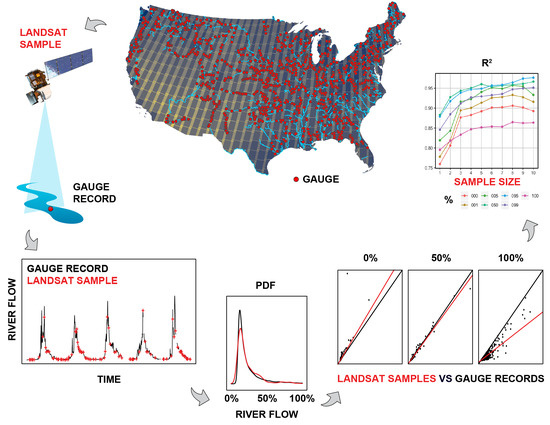
1. Introduction
Rivers serve as the chief source of renewable water to humans and to freshwater habitats [1] and thus they represent an important nexus between the water cycle, civilization, and aquatic ecology. Effective water resource management depends on the ability to monitor river systems and understand how they are responding to changes in climate and land use. While hydrological simulations can provide useful data for evaluating river system dynamics, they are often unable to resolve unpredictable processes and events, leading to high uncertainty, particularly when operating over large areas [2]. Observational monitoring of rivers is therefore essential for a complete understanding of the real-world complexities of river systems.
The stream gauge is the traditional instrument used for monitoring river hydrology. Gauges provide temporally continuous data that can be highly accurate given proper gauge maintenance. From gauge records, flow frequency distributions, or the frequency distribution of river flow through time, can be used to calculate return period and estimate future flood hazard under the assumption of stationarity [3]. However, gauges only monitor fixed points along river reaches and thus are unable to provide a comprehensive view of surface water hydrology across river networks [4]. Additionally, gauges tend to be biased in their geographic location, most often being installed along narrow, stable reaches, near populated regions, in developed countries, and on perennial river types [5]. Further, the availability of gauge data has been declining since the 1970s [6], limiting the ability to understand how changes in land use and the water cycle are impacting global rivers.
Satellite remote sensing of Earth’s rivers offers an alternative, complementary approach to in situ gauging [7]. Remote sensing data are often spatially continuous and thus can be used to observe an entire river network within the constraints of a given satellite’s payload and orbit. Remote sensing also enables non-intrusive measurement of rivers that avoids the inconsistencies associated with individually-maintained gauge stations. While optical remote sensing is the most popular method for studying rivers from space, it is susceptible to cloud cover, low sun angle, seasonal darkness, and nighttime conditions [8]. Other approaches like microwave remote sensing can be used to observe rivers during the day and night, and during almost all weather conditions [9,10,11], and high-resolution commercial imagery is emerging as a useful tool for unprecedented fine-scale monitoring of river and stream processes [12,13].
Satellite instruments cannot directly detect river discharge itself, but they can measure other properties of rivers that vary with discharge including river width [14], river height [15], and river velocity [16], as well as water quality [17]. Earth observation satellites have been operational since the early 1970s and have yielded long-term remote sensing data archives that serve as a valuable resource for monitoring rivers [18,19,20]. For example, remote sensing observations can be related to gauged discharge and can be used to build percentile-based rating curves [21,22]. However, the vast majority of Earth’s river reaches are ungauged [23] and for these ungauged reaches, the range of hydrological conditions that satellite data cover is uncertain. A satellite’s record is a discontinuous temporal sample of the overall population of hydrological conditions along rivers. However, the ability of satellite remote sensing data archives to represent flow frequency is unquantified. Does the satellite sample effectively represent flow frequency distribution in rivers?
Recent technological innovations have made this question more germane. Cloud computing image processing platforms like Google Earth Engine have substantially lowered the barriers to entry of planetary-scale analysis of entire satellite image archives [24]. These platforms have led to the development of freely-available global-scale maps of surface water occurrence and change from long-term aggregations of optical imagery [25,26] as well as open-source image processing algorithms that can be used to track changes in river morphology over decades [27]. Additionally, new global datasets of rivers including the Global River Widths from Landsat (GRWL) database [28], which contains the location and width of rivers observable by Landsat, allows for improved classification and analysis of rivers from satellites.
We are nearing the half-century anniversary of the first civilian satellite focused on Earth’s land surface (ERTS-1 launched in 1972 and later renamed Landsat 1). Indeed, Landsat is the longest running Earth observation satellite program and it is a standard source of remote sensing data for land cover characterization used in hydrological applications [29]. In particular the archives of Landsat 5, 7 and 8 (hereinafter simply referred to as Landsat), which all share the same Worldwide Reference System (WRS-2), contain freely-available, cross-calibrated sensor data with compatible spatial and temporal resolutions. Landsat provides ~30 m optical and infrared observations across a 185 km swath along a sun-synchronous near-polar 16 day repeat orbit. Thus, Landsat produces consistent multispectral imagery at a high spatial resolution but at a temporally sparse interval, particularly when cloud cover prevents land surface retrieval. We focus on Landsat here because it is the most commonly used remote sensing platform for studying surface water from space [8] and it has been the basis for several popular geospatial products for studying rivers [25,28,30,31,32].
However, an important unknown is whether the accumulated observations of rivers from Landsat, or the Landsat sample, correspond to the true population of hydrological conditions in rivers. If the available Landsat sample adequately captures the on-the-ground frequency distribution of river flow, then Landsat-based surveys of river characteristics can be interpreted to be representative of the hydrological conditions present along Earth’s rivers. Quantifying the ability of the Landsat archive to represent hydrological conditions, represented here by flow frequency, is motivated by several unexplored applications in the field of remote sensing of rivers. These include (1) using water occurrence information from the Landsat archive to estimate discharge by constructing river width-based rating curves; (2) using water occurrence information to quantify the seasonality of river and stream inundation extent, an important metric for estimating biogeochemical exchange between rivers and the atmosphere [33]; (3) using water color information to understand the variability and dynamics of river water quality [19].
If the Landsat archive is of adequate length or, in other words, if the Landsat sample size is large enough, then fundamental assumptions can be made regarding the representativeness of the Landsat record of hydrological conditions along Earth’s large rivers. Thus, given the long Landsat archive (Landsat 5 launched on 1 March 1984), we hypothesize that long-term aggregations of Landsat imagery capture the flow frequency of Earth’s large rivers. Here, we test this hypothesis by conducting a simple temporal sampling analysis of the United States Geological Survey (USGS) gauge records based on cloud-free overpass timing of Landsat 5, 7 and 8 (Figure 1). While a similar approach has been taken to predict the observational potential of the future Surface Water and Ocean Topography (SWOT) satellite mission [34], there has been no evaluation conducted for the widely used Landsat archive.
2. Materials and Methods
2.1. Gauge Data
We represent the true flow frequency of rivers using daily streamflow records from gauge stations in the United States (US) and operated by the USGS (Figure 1). To exclude gauges that are located on rivers too narrow to be observable by Landsat, we only consider the 1134 USGS gauges that were used to validate the Global River Widths from Landsat (GRWL) database [28]. These gauges (1) have upstream drainage areas larger than 1000 km2; (2) have records that span at least 10 years; (3) are located within 1 km Euclidean distance of a GRWL centerline; (4) are not immediately adjacent to lakes, reservoirs or river confluences (determined using the GRWL flag field and by visually examining each gauge location [28]); (5) have in situ river width data available [35]. We only analyze discharge records occurring between 1 March 1984 and 14 August 2019, because this time period spans the range of available data from the Landsat 5, 7 and 8 missions at the time of this study’s analysis. To help ensure a representative distribution of discharge at each gauge, we omit from our analysis 102 gauges that contain less than 5 years of discharge records within the 35 year study period. Additionally, because discharge conditions can be obscured by the presence of river ice [36], we exclude all gauge measurements that were taken when river ice was recorded at the gauge (USGS Quality Code set to “ice”). Similarly, we exclude discharge records that the USGS reported as provisional, estimated, underestimated, or overestimated (USGS Quality Code set to “p”, “E”, “<”, or “>”). Combined, these exclusions remove 5.2% of the daily discharge measurements but they produce a more accurate and representative discharge record for this study. The gauges used here are located on rivers, with a median width at mean annual discharge of 76 m and a first and third quartile of 50 to 117 m, respectively, as measured by the USGS [28].
2.2. Landsat Data
To assess the ability of Landsat to capture the true flow frequency distribution, we match coincident Landsat 5, 7, and 8 overpasses with daily discharge measurements at each USGS gauge over the 35-year study period (Figure 2a,c). Note that this matching process is idealized in that the discharge value at the gauge is exactly assigned to the corresponding Landsat image. This approach effectively assumes that river discharge can be accurately estimated from Landsat width measurements, an active field of research [7,22,27,37,38,39]. This simplifying assumption is a necessary first step that neglects potential errors in remote sensing and discharge algorithms, but allows for our stated focus on analyzing Landsat sampling capabilities. We conduct this Landsat availability analysis using the Google Earth Engine platform [24], which hosts the entire digitized Landsat archive. Each Landsat satellite observes the same location at least once every 16 days, although in areas with frequent cloud cover, the actual interval of cloud-free observations can be much longer (Figure 1). To account for the impact of cloud cover, we also determine when an available Landsat scene is cloud-free within a 500-m radius around the gauge. We use a 500-m radius around each gauge because this distance is longer than the corresponding in situ river width at mean discharge of all but 14 gauges considered in this study [28]. We identify clouds based on the USGS Landsat Bitwise Quality Assessment (BQA) product [40]. To account for the impact of the ETM+ Scan Line Corrector failure on data quality [41], we conservatively omit all Landsat 7 observation dates after 31 May 2003, when the failure occurred. In total, the number of observations considered in this analysis after excluding clouds and problematic gauge measurements is 327,177.
2.3. Statistical Comparison at Individual Gauges
At each individual USGS gauge, we compare the flow frequency distribution of the idealized Landsat sample to the flow frequency distribution of the daily gauge record (Figure 2). The upper panel in Figure 2 shows an example of where the Landsat sample and the gauge record have flow distributions that are relatively similar, whereas the lower panel shows an example where the Landsat sample does not represent the gauged flow distribution with high fidelity. We use the non-parametric Kolmogorov–Smirnov (K-S) test [42] to characterize the statistical difference between the Landsat sample and the daily record of flow at each gauge. We use a significance level of α = 0.05 for all statistical tests in this study.
Note that the K-S p-value is highly sensitive to sample size, causing it to be an impractical statistic for comparing across individual gauges. For example, a gauge with more Landsat observations (a larger sample size) is more likely to be considered significantly different than the same gauge with fewer observations (a smaller sample size), according to the K-S p-value [43,44]. Thus, the K-S p-value often yields contrary results, in which a large sample with a distribution that appears similar to that of its population will be considered to be significantly different (e.g., Figure 2a,b), while a small sample that appears to highly deviate from the gauge record will not be considered to be significantly different (e.g., Figure 2c,d). Due to this contradictory behavior, we do not place emphasis on the K-S p-value in this analysis but rather focus on the descriptive K-S D-statistic (KSD statistic), which provides a clear summary of the difference in flow frequency distributions between the Landsat sample and gauge record.
Additionally, we analyze the ability of Landsat to capture hydrological extremes at each individual gauge by determining the maximum and minimum percentile of gauged flows sampled by Landsat. We then explore potential factors affecting the ability of the Landsat sample to represent true flow frequency distributions across gauges including climate (cloudiness), watershed area and flow regime (flashiness). Flashiness is quantified according to the Richards–Baker Flashiness Index that sums the differences in daily flow divided by the total flow over a given time period [45]. This non-dimensional index is commonly used and has been observed to vary from 0 to ~1.5, although large rivers are generally less flashy and tend to exhibit index values of less than ~0.5 [34]. We correlate these factors with the KSD statistic using the Spearman rank correlation test [46] across all gauges and we examine the spatial patterns in the KSD statistic.
2.4. Statistical Comparison Across Multiple Gauges
To determine the ability of Landsat to represent river flow frequency across space, we compare the Landsat sample to the daily gauge record at different flow frequencies (Figure 2e). This approach tests whether different locations can be combined to represent flow frequency and is analogous to the classic hydrological concept of downstream hydraulic geometry [47]. In such a conceptual framework, the approach taken in Section 2.3 is equivalent to at-a-station hydraulic geometry. At each gauge, we calculate (1) discharge from the full gauge record and (2) discharge from the Landsat sample at multiple flow percentiles. Figure 2b,d shows two examples of calculating these two metrics at the 50th flow percentile (median flow). In addition to median flow, we calculate the two metrics at the following flow percentiles: 0% (minimum flow), 5%, 10%, 90%, 95%, and 100% (maximum flow).
For each of these percentiles, we compare the Landsat sample discharge to the gauge record discharge at every gauge using the non-parametric Mann–Whitney–Wilcoxon test (MWW) [48]. To avoid bias from outliers, we use the Theil–Sen median estimator [49] to derive a robust linear regression between the Landsat-sampled discharge and the gauge record discharge at each percentile. Additionally, we also calculate relative root mean square error,
and the relative bias,
where N is the total number of gauges used in this study, Qi,j is the flow (m3s−1) from the Landsat sample distribution at a given percentile, j, at gauge i and is the flow from the gauge distribution at the same percentile and same gauge. By comparing the Landsat sample to the gauge record across all the gauges at each selected percentile, we evaluate the ability of Landsat to represent a given flow frequency through spatial averaging.
2.5. Minimum Length of Landsat Observations
We expect that the ability of satellites to effectively represent river flow frequency is related to the length of the observational archive and hence the sample size. Theoretically, longer sampling periods enable better capture of the flow frequency distribution during the sample period. To examine the effect of observation length on Landsat’s capacity to represent flow frequency, we simulated different observation period lengths over which Landsat-sampled discharge from the gauge record. For each gauge in our analysis, we created 50 random permutations of a continuous temporal range with an n year duration (n = 1, 2, 3, …, 10). To allow for random permutations of a 10 year period, we only included gauges that contained more than 15 years of continuous data (N = 927). Within each temporal range, we compared the Landsat-sampled flows and those from daily gauge records from the same period. Specifically, we calculated flow values at 0%, 1%, 5%, 50%, 95%, 99%, and 100% percentiles. From these data, we calculated the coefficient of determination (R2), relative error metrics (rBias, rMAE, and rRMSE), and absolute error metrics (Bias, MAE, and RMSE). Together, these statistics help characterize the ability of Landsat to represent flow conditions with increasing observation duration.
3. Results
3.1. How Well Can the Landsat Archive Capture Flow Conditions at Individual Gauges?
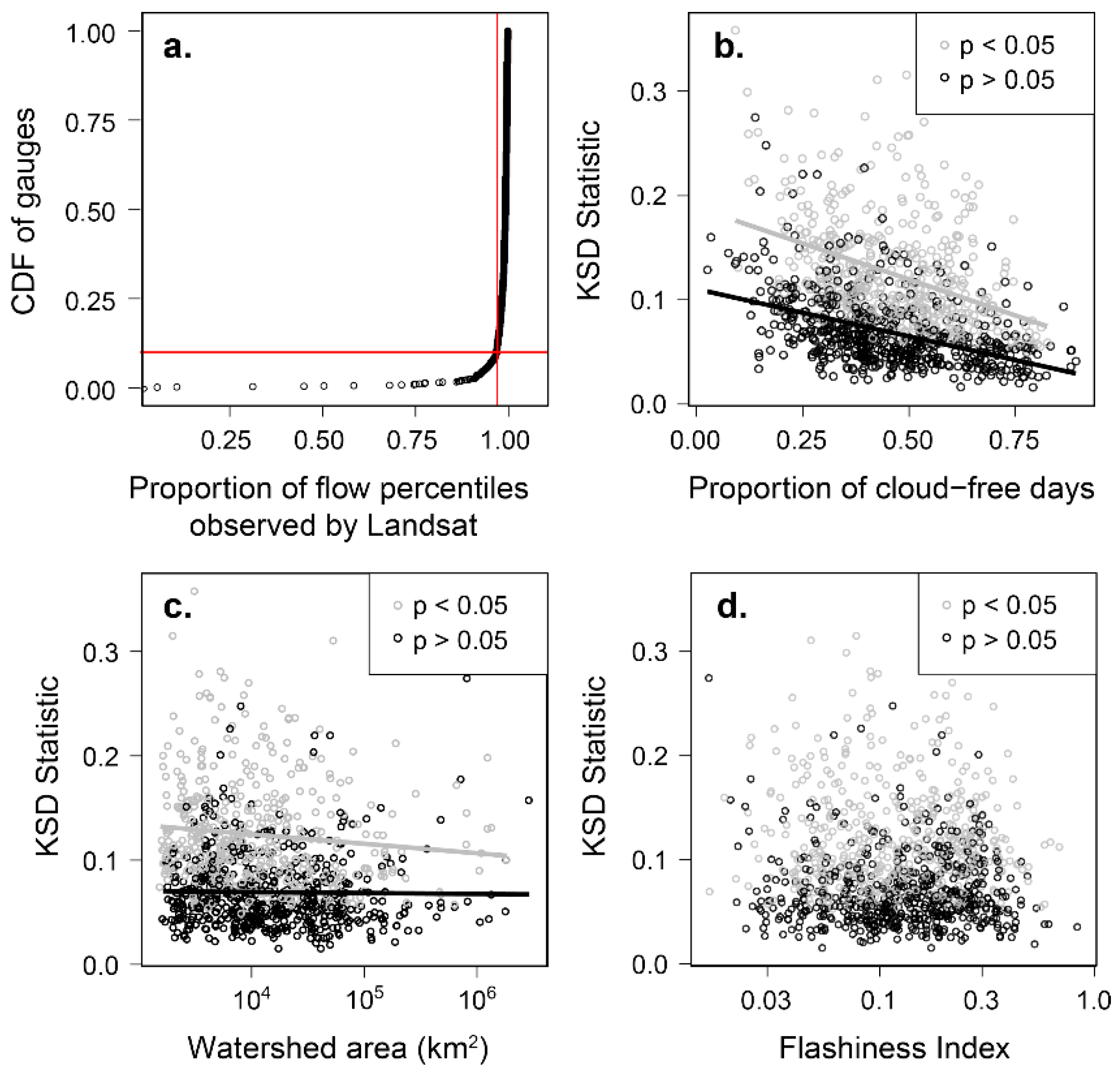
We find that the Landsat archive contains observations corresponding to the near full range of discharge conditions for the vast majority of gauges (Figure 3a). For example, at 90% of the study gauges, the idealized Landsat sample captures at least 97% of the full range of discharge percentiles recorded by the gauge. The majority of gauges (55%) show no significant difference between the Landsat sample and the gauge record of flow according to the K-S p-value at the 95% confidence interval. However, as previously noted, the K-S p-value is exceedingly sensitive to sample size and often produces contradictory results when comparing samples of different sizes, as we do here. On the other hand, the descriptive KSD statistic, which does not exhibit this contradictory behavior, ranges from 0.016 to 0.36, with a median value of 0.083. Among the sites with no significant difference between the Landsat-sampled and gauged flow frequency, the KSD statistic ranged from 0.016 to 0.27, with a median value of 0.06. Thus, while there is considerable variation in the potential ability of Landsat to reconstruct flow frequency from gauge to gauge, the average difference between the idealized Landsat sample and the gauge flow frequency distribution is small.
To determine potential drivers of Landsat’s ability to capture river flow frequency, we examine correlations between the KSD statistic and the environmental variables of cloudiness, watershed area, and flow flashiness. We find a negative correlation (p < 0.001) between the proportion of cloud-free observations at a gauge and the KSD statistic (Figure 3b). This pattern is evident for locations where there is a statistically significant difference between the Landsat sample and the gauge record (gray points in Figure 3b) as well as locations that exhibit no significant difference (black points in Figure 3b; Spearman rank correlation coefficients of r = −0.40 and r = −0.47, respectively). We also find a weak negative correlation between the KSD statistic and watershed area (r = −0.09 and −0.16; p = 0.02 and p < 0.001; Figure 3c) for locations with significant difference and locations with a significant difference, respectively. Conversely, we find no significant correlations between flow flashiness and the KSD statistic at sites with statistically significant differences (r = 0.012, p = 0.78) nor at sites with statistically insignificant differences (r = 0.018, p = 0.66; Figure 3d). Landsat-observable rivers are large and span a relatively narrow range of the Richards–Baker Flashiness Index, from 0.016 to 0.84, compared to small streams that can vary up to 1.5 [34]. The lack of correlation between flashiness and the KSD statistic implies that flow regimes on large Landsat-observable rivers do not affect Landsat’s ability to capture flow frequency distribution. We find no readily apparent spatial patterns in the D-statistic (see Figure S1 for an interactive map showing flow frequency distributions of the Landsat sample and the gauge record for each stream gauge). While more sophisticated statistical approaches could be employed to predict locations where Landsat best captures river flow frequency, this task is beyond the scope of this study.
3.2. How Well Can the Landsat Archive Capture Flow Conditions across Multiple Gauges?
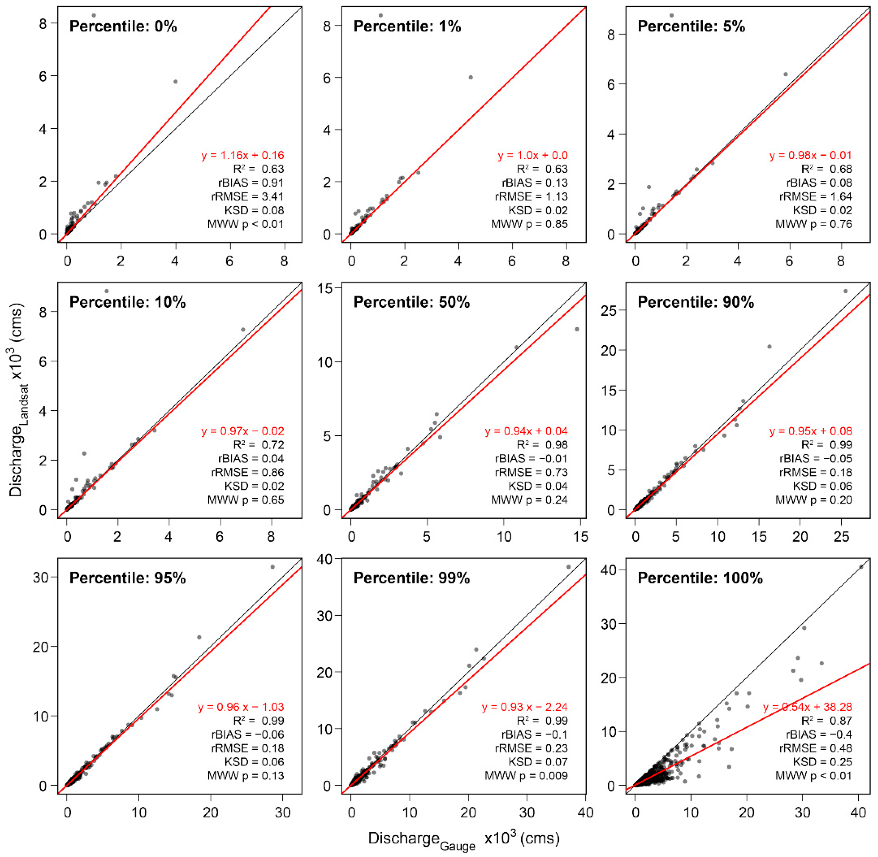
Comparing the Landsat sample to the gauge record across all gauge stations reveals consistent patterns between a given flow percentile and the ability of Landsat to potentially represent flow at that percentile (Figure 4). For a wide range of flows (i.e., the 1% through the 95% percentiles in Figure 4), we find no statistically significant difference between the Landsat sample and the full gauge record according to the MWW test. Thus, except for extreme hydrological conditions like maximum and minimum flow, the idealized Landsat sample is not statistically different from the daily flow measured by multiple gauges (α = 0.05). Error metrics tend to be highest at extreme flow conditions and lowest at median flow. For intermediate percentiles that show no statistically significant difference, rRMSE values range from 12% to 78% and rBIAS values range from −6.4% to 8%.
Examining the error statistics of the extreme flow percentiles yields additional insights. At minimum flow, the Landsat sample always either matches or overestimates minimum flow, as seen by the points always being above the 1:1 line in the 0% percentile panel of Figure 4, resulting in a high positive relative bias of 200%. Conversely, at maximum flow, the Landsat sample either equals or underestimates maximum flow, producing a negative relative bias of −31%. These underestimates tend to increase in magnitude with increasing discharge (errors exhibit heteroscedasticity), resulting in a Theil–Sen median estimator that significantly deviates from unity at the 100% percentile (red line). These patterns also persist at the 99% percentile, in which the Landsat sample tends to underestimate discharge, albeit to a lesser degree than at maximum flow.
3.3. What Is the Minimum Length of Landsat Observations Needed to Represent Flow Frequency?
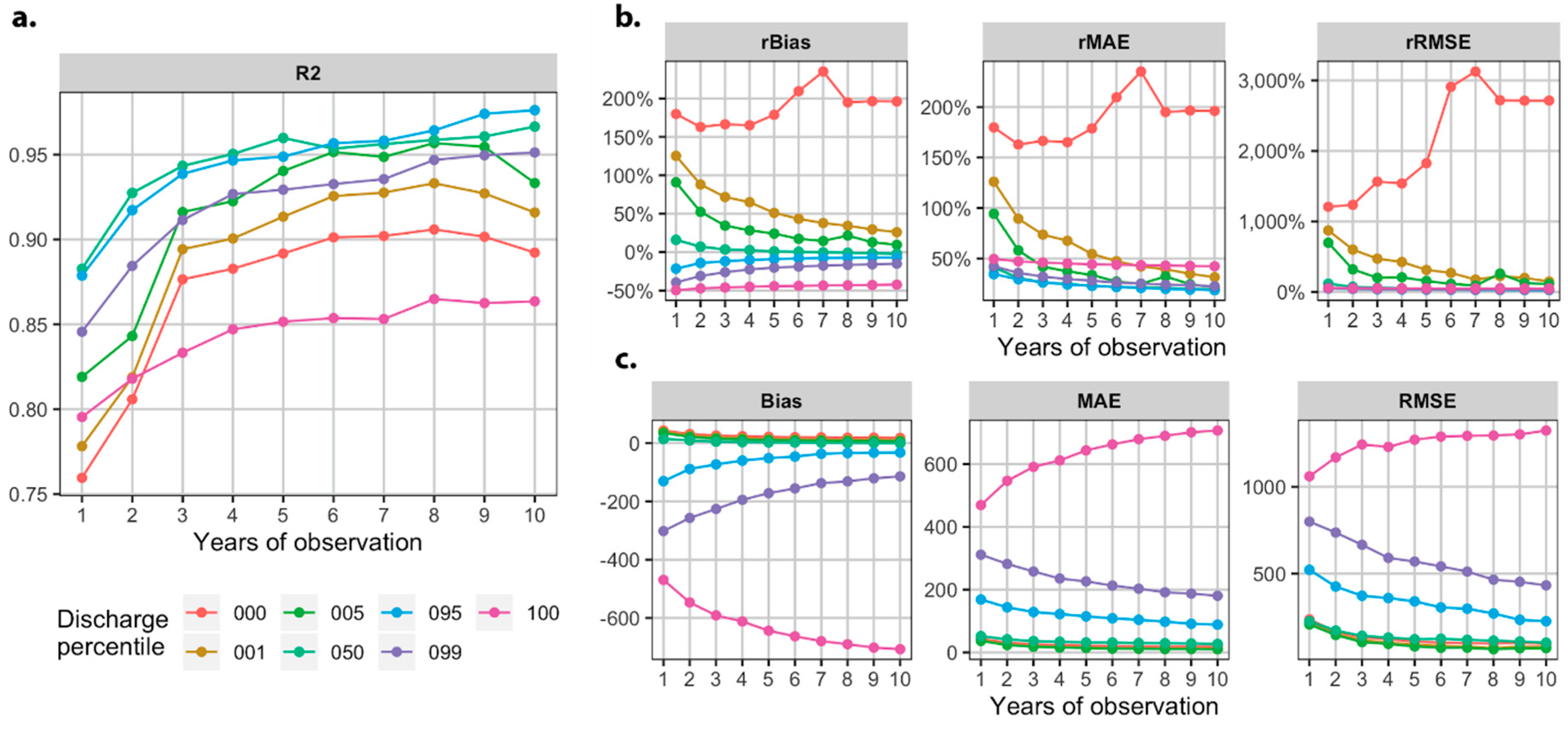
Our findings confirm that long periods of Landsat observation correspond with an improved ability of the Landsat archive to contain observations that can effectively represent river flow frequency. Generally, after 3 years of Landsat observation, all percentiles except for minimum and maximum flow are in close agreement with the reference values derived from the gauge record, with R2 values above 0.9 (Figure 5a). Moreover, with the exception of minimum and maximum flow, we find a general trend of decreasing relative error statistics (rBias, rMAE, and rRMSE; Figure 5b) and absolute error statistics (Bias, MAE, RMSE; Figure 5c) with increasing duration of observation. Thus, as satellite observation duration increases, the distribution of flow frequency observed by Landsat expectedly converges with the flow frequency of the daily gauge record, except for extreme flows like minimum and maximum discharge.
Additionally, our results reveal that the degree of increasing similarity between the Landsat sample and the gauge record flow frequency distributions strongly depends on the flow percentile being studied. With increasing observation duration, smaller percentile flows generally show a more dramatic improvement in performance relative to larger flows. For example, Figure 5a shows a more substantial increase in R2 for low flow percentiles (0%, 1%, and 5% flow) at a 3 year duration relative to the larger flow percentiles. This pattern also persists for the relative error metrics whereby the decreasing trend is greatest in smaller percentiles, with the exception of minimum and maximum flow. We note that low flow frequencies correspond to higher relative errors compared to higher flow frequencies, likely because of their smaller denominators in Equations (1) and (2). Conversely, high flow frequencies correspond to higher absolute error metrics relative to lower flow frequencies and the non-linear gap between the percentile curves may result from the positive skewness of flow frequency distributions in most rivers.
4. Discussion
4.1. Interpretations of Primary Findings
Our results indicate that Landsat can effectively capture river flow frequency over large spatial areas given an adequate duration of observation and accurate remote sensing and discharge algorithms. Although Landsat’s sampling capability varies at individual gauge sites, we find that spatially averaging over multiple gauges enables effective representation of flow frequency, with the exception of extremely high and low flows (Figure 4). Landsat more aptly captures flow frequency at the lowest flows rather than at the highest flows, likely because of the positive skew characteristic of flow frequency distributions (e.g., Figure 2b). Small changes in flow frequency at the highest flows represent large variations in discharge that are difficult to capture due to the 16 day repeat orbit of Landsat. Cloudy conditions often accompany high flows, which further inhibits Landsat’s ability to characterize the frequency of high flow events. The duration of observation also plays an important role in the ability of Landsat to capture river flow frequency. As expected, a longer observation duration will produce a better representation of river flow frequency, albeit with diminishing returns (Figure 5). Several error metrics initially improve rapidly with time until approximately a 3 year duration, after which they improve more gradually. Thus, we suggest that at least 3 years of Landsat observations should be aggregated before they adequately contain observations representative of river flow frequency.
4.2. Implications for River Remote Sensing Applications
River flow frequency analysis is a key tool for a variety of hydrological applications including flood hazard and risk evaluations, hydraulic engineering, and water resources management [50,51]. Flow frequency is also related to a river’s water quality and distribution of freshwater habitats [52,53,54]. While satellite remote sensing cannot measure discharge directly, it can measure other attributes of rivers that scale with discharge including river morphology and water quality [47,55]. For example, Landsat can observe surface water inundation extent from which river surface area and width can be extracted, which both scale with discharge [27,56,57,58].
This study’s findings indicate river water occurrence data derived from long-term aggregations of Landsat observations correspond to the flow frequency of Earth’s large rivers. For example, on average, median river width derived from long-term temporal composites of classified Landsat data [25,26] corresponds to median river flow. Our results also indicate that these same relationships can be extended to a wide range of flow frequencies, except for extremely high and low flows. This result has key utility for developing percentile-based width rating curves for estimating discharge [14,22] or for estimating variability in river surface area [59]. We emphasize that at any single given location, these relationships do not necessarily apply but rather that these relationships are valid when averaging over space. Thus, applying at-a-station hydraulic geometry [47] at individual single cross-sections solely from Landsat water occurrence data may often be invalid. However, our results suggest that developing at-a-station hydraulic geometry relationships across multiple cross-sections over a large area is valid for non-extreme flow frequencies and given an adequate Landsat sample size with potential implications for remote sensing of discharge approaches [15,37,38,39].
Our results also have implications for riparian ecology and river water quality applications. Flow is a “master” variable in river ecology and water quality [54] and, like river width and surface area, Landsat can also measure water quality parameters [31,60]. Specifically, Landsat imagery is commonly paired with in situ water samples to derive empirical relationships with optically-active constituents such as suspended sediment concentrations [61,62], chlorophyll-a [60,63], and colored dissolved organic matter (CDOM) [64,65]. While these water quality parameters generally vary with discharge, the relationship between river flow and water quality varies. Suspended sediment generally increases non-linearly with flow [66] but chlorophyll-a and CDOM can increase, decrease, or vary independently of flow depending on river size, season, and watershed properties [67,68,69,70]. Understanding flow conditions captured by satellite observations is therefore important for deriving representative surveys of river water quality measurements. The most extreme flow events are rarely observed by Landsat, but Landsat observes a wider range of flows (97% of flow percentiles at 90% of gauges) than well-designed water quality field sampling programs which sample 80% of flow percentiles at best [71]. Thus, as remote sensing of water quality methods typically relies on in situ field measurements, it is critical that field sampling programs collect measurements at high and low flows to match the wide range of hydrological conditions captured by Landsat observations.
4.3. Limitations and Future Directions
While the results of this study are encouraging for river remote sensing applications, our study does have limitations. First, we assume that daily discharge measured from the USGS study gauges represents the true flow frequency of rivers, but river gauges are biased in their placement and fluctuations in river discharge often can occur over subdaily timescale [5,72]. Related to this point, our results may differ in regions outside the US, which have dissimilar conditions. The gauge stations used in this study measure the majority (52%) of US Landsat-observable river reaches but only 6.6% of Earth’s observable rivers are located within the US, according to the GRWL database [28]. Future work could explore this uncertainty by using an international gauge database [73] or a global hydrological simulation [74] to sample streamflow worldwide. Second, we emphasize that Landsat will not necessarily produce a representative sample of flow at any given single location along a river network. However, our results indicate that, given an adequate period of observation, spatially-averaged Landsat observations can capture flow frequency distribution over large spatial areas. Further, Landsat does not adequately capture minimum and maximum flow conditions in most locations. Third, while this study does not assume stationarity, we emphasize that river flow frequency is non-stationary such that flow frequencies derived over one time period cannot necessarily be used to infer flow frequencies over another period [3]. Finally, this study does not consider the uncertainty associated with the Landsat remote sensing measurements themselves. So, while we find that the timing of Landsat observations is adequate to capture river flow frequency, the ability of Landsat to accurately measure the parameter of interest (e.g., river width, suspended sediment concentration, discharge) itself remains unconstrained here. Constraining this uncertainty is application and algorithm specific [7,20] and beyond the scope of this analysis. Additionally, determining the drivers of the heterogeneity in Landsat’s ability to represent flow frequency from location to location (Figure S1) is a recommended topic for further research.
Similar approaches to this study may be used to understand river sampling capabilities of satellite missions other than Landsat. Satellite programs with optical sensors and shorter revisit times, such as Sentinel 2 (2–5 days) and Planet (~1 day), likely capture river flow frequency over a shorter study duration, although this advantage of more frequent retrieval will be bottlenecked by persistent cloud cover in some regions. Other sensor technologies enable remote sensing of rivers over a broader array of atmospheric and solar illumination conditions. Indeed, thermal, passive microwave, radar and lidar remote sensing have distinct advantages over optical remote sensing and can provide alternative observations of river systems. Similar to this study, a recent analysis found that 3 years of SWOT data were sufficient to represent the flow frequency distribution over the Mississippi River basin [34]. SWOT will have a longer repeat orbit (21 days) and narrower swath width (100 km) than Landsat but these attributes are counterbalanced by the ability of its Ka-band radar instrument to collect surface returns during cloudy and nighttime conditions [11].
5. Conclusions
This study’s findings show that the Landsat archive can effectively represent river flow frequency over large areas given an adequate period of observation and accurate remote sensing and discharge algorithms. At individual locations, the ability of Landsat to capture flow frequency in large rivers is positively correlated with the cloud occurrence, weakly correlated with watershed area, and does not correlate with flow flashiness (Figure 3; Figure S1). While the Landsat record captures a wide range of flow conditions (97% of the flow percentiles at 90% of sites), its ability to capture the flow frequency distribution varies widely from location to location (KSD statistic ranges from 0.016–0.36). This implies that, at any single site along a river, the Landsat archive cannot be assumed to adequately capture flow frequency. Nevertheless, we find that spatially averaging over multiple locations effectively enables representation of hydrological conditions at a given flow frequency, with the exception of hydrological extremes like maximum and minimum flow (α = 0.5; Figure 4). Such an averaging process could hence be used to improve existing Landsat-based discharge algorithms. Landsat can better capture flow frequency at the lowest flows than at the highest flows likely because of the positive skew characteristic of river flow frequency distributions. We also find that a longer Landsat observation time period positively impacts the representation of river flow frequency, albeit with diminishing returns with increasing observation time (Figure 5). We suggest that, on average, a minimum of 3 years of aggregated observations is necessary if Landsat is used to reconstruct flow frequency distribution. We emphasize that this analysis only considers the timing of Landsat observations in relation to river flow frequency and does not consider the ability of Landsat to accurately measure the parameter of interest (e.g., river width, suspended sediment, discharge). We also note that the gauges used in this analysis only measure a relatively small portion of the global observable river network, solely located within the United States. Regardless, the results of this study support the hypothesis that long-term aggregations of Landsat data can be used to capture the flow frequency of Earth’s large rivers. Thus, Landsat-based surveys of river characteristics can be interpreted to be representative of the hydrological conditions present along Earth’s large rivers, with wide-ranging utility for river hydrology, water quality, and ecology.
Supplementary Materials
The following are available online at https://0-www-mdpi-com.brum.beds.ac.uk/2072-4292/12/9/1510/s1, Figure S1: Interactive map showing values of the KSD statistic over each gauge and the flow frequency distribution of the Landsat sample and the gauge record. The data produced in this study are openly available under a Creative Commons Attribution License at https://0-doi-org.brum.beds.ac.uk/10.5281/zenodo.3817346. The software used to analyze the data and produce the figures is available at https://github.com/geoallen/ROTFL/ under a Berkeley Software Distribution 3-Clause License.
Author Contributions
Conceptualization, G.H.A.; methodology, all authors; formal analysis, G.H.A., X.Y., J.G., and M.R.; data curation, J.H. and G.H.A.; writing—original draft preparation, G.H.A., X.Y., J.G., J.H., C.H.D., and M.R.; writing—review and editing, G.H.A., X.Y., J.G., J.H., C.H.D., and M.R.; visualization, G.H.A., M.R., X.Y., and J.G.; supervision, G.H.A. All authors have read and agreed to the published version of the manuscript.
Funding
This research was funded by NASA THP grant #NNH17ZDA001N. X.Y. was funded by a subcontract from the SWOT Project Office at the NASA/Caltech Jet Propulsion Laboratory to Tamlin M. Pavelsky and J.G. was funded by NSF-EAR Postdoctoral Fellowship grant #1806983. C.H.D. was supported by the Jet Propulsion Laboratory, California Institute of Technology, under a contract with NASA.
Acknowledgments
We thank Cassandra Nickles and Edward Beighley for providing helpful feedback during the initial phase of this project.
Conflicts of Interest
The authors declare no conflict of interest. The funders had no role in the design of the study; in the collection, analyses, or interpretation of data; in the writing of the manuscript, or in the decision to publish the results.
References
- Vorosmarty, C.J.; McIntyre, P.B.; Gessner, M.O.; Dudgeon, D.; Prusevich, A.; Green, P.; Glidden, S.; Bunn, S.E.; Sullivan, C.A.; Liermann, C.R.; et al. Global threats to human water security and river biodiversity. Nature 2010, 467, 555–561. [Google Scholar] [CrossRef] [PubMed]
- Wood, E.F.; Roundy, J.K.; Troy, T.J.; van Beek, L.P.H.; Bierkens, M.F.P.; Blyth, E.; de Roo, A.; Döll, P.; Ek, M.; Famiglietti, J.; et al. Hyperresolution global land surface modeling: Meeting a grand challenge for monitoring Earth’s terrestrial water. Water Resour. Res. 2011, 47. [Google Scholar] [CrossRef]
- Milly, P.C.D.; Betancourt, J.; Falkenmark, M.; Hirsch, R.M.; Kundzewicz, Z.W.; Lettenmaier, D.P.; Stouffer, R.J. Stationarity Is Dead: Whither Water Management? Science 2008, 319, 573. [Google Scholar] [CrossRef] [PubMed]
- Alsdorf, D.; Bates, P.; Melack, J.; Wilson, M.; Dunne, T. Spatial and temporal complexity of the Amazon flood measured from space. Geophys. Res. Lett. 2007, 34, L08402. [Google Scholar] [CrossRef]
- Park, C.C. World-wide variations in hydraulic geometry exponents of stream channels: An analysis and some observations. J. Hydrol. 1977, 33, 133–146. [Google Scholar] [CrossRef]
- Gudmundsson, L.; Do, H.X.; Leonard, M.; Westra, S. The Global Streamflow Indices and Metadata Archive (GSIM)—Part 2: Quality control, time-series indices and homogeneity assessment. Earth Syst. Sci. Data 2018, 10, 787–804. [Google Scholar] [CrossRef] [Green Version]
- Gleason, J.C.; Durand, T.M. Remote Sensing of River Discharge: A Review and a Framing for the Discipline. Remote Sens. 2020, 12, 1107. [Google Scholar] [CrossRef] [Green Version]
- Huang, C.; Chen, Y.; Zhang, S.; Wu, J. Detecting, Extracting, and Monitoring Surface Water from Space Using Optical Sensors: A Review. Rev. Geophys. 2018, 56, 333–360. [Google Scholar] [CrossRef]
- Twele, A.; Cao, W.; Plank, S.; Martinis, S. Sentinel-1-based flood mapping: A fully automated processing chain. Int. J. Remote Sens. 2016, 37, 2990–3004. [Google Scholar] [CrossRef]
- Lan Anh, D.T.; Aires, F. River Discharge Estimation based on Satellite Water Extent and Topography: An Application over the Amazon. J. Hydrometeorol. 2019, 20, 1851–1866. [Google Scholar] [CrossRef]
- Biancamaria, S.; Lettenmaier, D.P.; Pavelsky, T.M. The SWOT Mission and Its Capabilities for Land Hydrology. Surv. Geophys. 2016, 37, 307–337. [Google Scholar] [CrossRef] [Green Version]
- Cooley, W.S.; Smith, C.L.; Stepan, L.; Mascaro, J. Tracking Dynamic Northern Surface Water Changes with High-Frequency Planet CubeSat Imagery. Remote Sens. 2017, 96, 1306. [Google Scholar] [CrossRef] [Green Version]
- Vanderhoof, K.M.; Burt, C. Applying High-Resolution Imagery to Evaluate Restoration-Induced Changes in Stream Condition, Missouri River Headwaters Basin, Montana. Remote Sens. 2018, 10, 913. [Google Scholar] [CrossRef] [Green Version]
- Smith, L.C.; Pavelsky, T.M. Estimation of river discharge, propagation speed, and hydraulic geometry from space: Lena River, Siberia. Water Resour. Res. 2008, 44, W03427. [Google Scholar] [CrossRef]
- Tourian, M.J.; Schwatke, C.; Sneeuw, N. River discharge estimation at daily resolution from satellite altimetry over an entire river basin. J. Hydrol. 2017, 546, 230–247. [Google Scholar] [CrossRef]
- Kääb, A.; Altena, B.; Mascaro, J. River-ice and water velocities using the Planet optical cubesat constellation. Hydrol. Earth Syst. Sci. 2019, 23, 4233–4247. [Google Scholar] [CrossRef] [Green Version]
- Onderka, M.; Pekárová, P. Retrieval of suspended particulate matter concentrations in the Danube River from Landsat ETM data. Sci. Total Environ. 2008, 397, 238–243. [Google Scholar] [CrossRef]
- Smith, L.C. Satellite remote sensing of river inundation area, stage, and discharge: A review. Hydrol. Process. 1997, 11, 1427–1439. [Google Scholar] [CrossRef]
- Topp, N.S.; Pavelsky, M.T.; Jensen, D.; Simard, M.; Ross, R.V.M. Research Trends in the Use of Remote Sensing for Inland Water Quality Science: Moving Towards Multidisciplinary Applications. Water 2020, 12, 169. [Google Scholar] [CrossRef] [Green Version]
- Piégay, H.; Arnaud, F.; Belletti, B.; Bertrand, M.; Bizzi, S.; Carbonneau, P.; Dufour, S.; Liébault, F.; Ruiz-Villanueva, V.; Slater, L. Remotely sensed rivers in the Anthropocene: State of the art and prospects. Earth Surf. Process. Landf. 2020, 45, 157–188. [Google Scholar] [CrossRef]
- Tourian, M.J.; Sneeuw, N.; Bárdossy, A. A quantile function approach to discharge estimation from satellite altimetry (ENVISAT). Water Resour. Res. 2013, 49, 4174–4186. [Google Scholar] [CrossRef]
- Pavelsky, T.M. Using width-based rating curves from spatially discontinuous satellite imagery to monitor river discharge. Hydrol. Process. 2014. [Google Scholar] [CrossRef]
- Pavelsky, T.M.; Durand, M.T.; Andreadis, K.M.; Beighley, R.E.; Paiva, R.C.D.; Allen, G.H.; Miller, Z.F. Assessing the potential global extent of SWOT river discharge observations. J. Hydrol. 2014, 519 Pt B, 1516–1525. [Google Scholar] [CrossRef]
- Gorelick, N.; Hancher, M.; Dixon, M.; Ilyushchenko, S.; Thau, D.; Moore, R. Google Earth Engine: Planetary-scale geospatial analysis for everyone. Big Remote Sensed Data Tools Appl. Exp. 2017, 202, 18–27. [Google Scholar] [CrossRef]
- Pekel, J.-F.; Cottam, A.; Gorelick, N.; Belward, A.S. High-resolution mapping of global surface water and its long-term changes. Nature 2016, 540, 418–422. [Google Scholar] [CrossRef]
- Pickens, A.H.; Hansen, M.C.; Hancher, M.; Stehman, S.V.; Tyukavina, A.; Potapov, P.; Marroquin, B.; Sherani, Z. Mapping and sampling to characterize global inland water dynamics from 1999 to 2018 with full Landsat time-series. Remote Sens. Environ. 2020, 243, 111792. [Google Scholar] [CrossRef]
- Yang, X.; Pavelsky, T.M.; Allen, G.H.; Donchyts, G. RivWidthCloud: An Automated Google Earth Engine Algorithm for River Width Extraction from Remotely Sensed Imagery. IEEE Geosci. Remote Sens. Lett. 2019, 1–5. [Google Scholar] [CrossRef]
- Allen, G.H.; Pavelsky, T.M. Global extent of rivers and streams. Science 2018. [Google Scholar] [CrossRef] [Green Version]
- Lettenmaier, D.P.; Alsdorf, D.; Dozier, J.; Huffman, G.J.; Pan, M.; Wood, E.F. Inroads of remote sensing into hydrologic science during the WRR era. Water Resour. Res. 2015, 51, 7309–7342. [Google Scholar] [CrossRef]
- Jones, W.J. Improved Automated Detection of Subpixel-Scale Inundation—Revised Dynamic Surface Water Extent (DSWE) Partial Surface Water Tests. Remote Sens. 2019, 11, 374. [Google Scholar] [CrossRef] [Green Version]
- Ross, M.R.V.; Topp, S.N.; Appling, A.P.; Yang, X.; Kuhn, C.; Butman, D.; Simard, M.; Pavelsky, T.M. AquaSat: A Data Set to Enable Remote Sensing of Water Quality for Inland Waters. Water Resour. Res. 2019, 55. [Google Scholar] [CrossRef]
- Yamazaki, D.; Ikeshima, D.; Sosa, J.; Bates, P.D.; Allen, G.H.; Pavelsky, T.M. MERIT Hydro: A High-Resolution Global Hydrography Map Based on Latest Topography Dataset. Water Resour. Res. 2019, 55, 5053–5073. [Google Scholar] [CrossRef] [Green Version]
- Raymond, P.A.; Hartmann, J.; Lauerwald, R.; Sobek, S.; McDonald, C.; Hoover, M.; Butman, D.; Striegl, R.; Mayorga, E.; Humborg, C.; et al. Global carbon dioxide emissions from inland waters. Nature 2013, 503, 355–359. [Google Scholar] [CrossRef] [PubMed] [Green Version]
- Nickles, C.; Beighley, E.; Zhao, Y.; Durand, M.; David, C.; Lee, H. How Does the Unique Space-Time Sampling of the SWOT Mission Influence River Discharge Series Characteristics? Geophys. Res. Lett. 2019, 46, 8154–8161. [Google Scholar] [CrossRef]
- Allen, G.H.; Pavelsky, T.M. Patterns of river width and surface area revealed by the satellite-derived North American River Width data set. Geophys. Res. Lett. 2015, 42, 395–402. [Google Scholar] [CrossRef]
- Yang, X.; Pavelsky, T.M.; Allen, G.H. The past and future of global river ice. Nature 2020, 577, 69–73. [Google Scholar] [CrossRef]
- Gleason, C.J.; Smith, L.C. Toward global mapping of river discharge using satellite images and at-many-stations hydraulic geometry. Proc. Natl. Acad. Sci. USA 2014, 111, 4788–4791. [Google Scholar] [CrossRef] [Green Version]
- Feng, D.; Gleason, C.J.; Yang, X.; Pavelsky, T.M. Comparing Discharge Estimates Made via the BAM Algorithm in High-Order Arctic Rivers Derived Solely from Optical CubeSat, Landsat, and Sentinel-2 Data. Water Resour. Res. 2019, 55, 7753–7771. [Google Scholar] [CrossRef]
- Durand, M.; Gleason, C.J.; Garambois, P.A.; Bjerklie, D.; Smith, L.C.; Roux, H.; Rodriguez, E.; Bates, P.D.; Pavelsky, T.M.; Monnier, J.; et al. An intercomparison of remote sensing river discharge estimation algorithms from measurements of river height, width, and slope. Water Resour. Res. 2016, 52, 4527–4549. [Google Scholar] [CrossRef] [Green Version]
- Foga, S.; Scaramuzza, P.L.; Guo, S.; Zhu, Z.; Dilley, R.D.; Beckmann, T.; Schmidt, G.L.; Dwyer, J.L.; Joseph Hughes, M.; Laue, B. Cloud detection algorithm comparison and validation for operational Landsat data products. Remote Sens. Environ. 2017, 194, 379–390. [Google Scholar] [CrossRef] [Green Version]
- Maxwell, S.K.; Schmidt, G.L.; Storey, J.C. A multi-scale segmentation approach to filling gaps in Landsat ETM+ SLC-off images. Int. J. Remote Sens. 2007, 28, 5339–5356. [Google Scholar] [CrossRef]
- Massey, F.J. The Kolmogorov-Smirnov Test for Goodness of Fit. J. Am. Stat. Assoc. 1951, 46, 68–78. [Google Scholar] [CrossRef]
- Fasano, G.; Franceschini, A. A multidimensional version of the Kolmogorov–Smirnov test. Mon. Not. R. Astron. Soc. 1987, 225, 155–170. [Google Scholar] [CrossRef]
- Crutcher, H.L. A Note on the Possible Misuse of the Kolmogorov-Smirnov Test. J. Appl. Meteorol. 1975, 14, 1600–1603. [Google Scholar] [CrossRef] [Green Version]
- Baker, D.B.; Richards, R.P.; Loftus, T.T.; Kramer, J.W. A new flashiness index: Characteristics and applications to midwestern rivers and streams. JAWRA J. Am. Water Resour. Assoc. 2004, 40, 503–522. [Google Scholar] [CrossRef]
- Spearman, C. The Proof and Measurement of Association between Two Things. Am. J. Psychol. 1904, 15, 72–101. [Google Scholar] [CrossRef]
- Leopold, L.B.; Maddock, T., Jr. The Hydraulic Geometry of Stream Channels and Physiographic Implications; US Government Printing Office: Washington, DC, USA, 1953; p. 57.
- Mann, H.B.; Whitney, D.R. On a Test of Whether one of Two Random Variables is Stochastically Larger than the Other. Ann. Math. Stat. 1947, 18, 50–60. [Google Scholar] [CrossRef]
- Sen, P.K. Estimates of the Regression Coefficient Based on Kendall’s Tau. J. Am. Stat. Assoc. 1968, 63, 1379–1389. [Google Scholar] [CrossRef]
- Chow, V.T.; Maidment, D.R.; Mays, L.W. Applied Hydrology; McGraw-Hill Series in Water Resources and Environmental Engineering; McGraw-Hill: New York, NY, USA, 1988; ISBN 0-07-010810-2. [Google Scholar]
- Rao, A.R.; Hamed, K.H. Flood Frequency Analysis, 1st ed.; CRC Press: Boca Raton, FL, USA, 2000; ISBN 978-0-8493-0083-7. [Google Scholar]
- Bunn, S.E.; Arthington, A.H. Basic Principles and Ecological Consequences of Altered Flow Regimes for Aquatic Biodiversity. Environ. Manag. 2002, 30, 492–507. [Google Scholar] [CrossRef] [Green Version]
- Nilsson, C.; Renöfält, B.M. Linking Flow Regime and Water Quality in Rivers. Ecol. Soc. 2008, 13, 18. [Google Scholar] [CrossRef] [Green Version]
- Poff, N.L.; Allan, J.D.; Bain, M.B.; Karr, J.R.; Prestegaard, K.L.; Richter, B.D.; Sparks, R.E.; Stromberg, J.C. The natural flow regime. BioScience 1997, 47, 769–784. [Google Scholar] [CrossRef]
- Rijn, L.C. van Sediment Transport, Part II: Suspended Load Transport. J. Hydraul. Eng. 1984, 110, 1613–1641. [Google Scholar] [CrossRef]
- Hou, J.; van Dijk, A.I.J.M.; Renzullo, L.J.; Vertessy, R.A.; Mueller, N. Hydromorphological attributes for all Australian river reaches derived from Landsat dynamic inundation remote sensing. Earth Syst. Sci. Data 2019, 11, 1003–1015. [Google Scholar] [CrossRef] [Green Version]
- Isikdogan, F.; Bovik, A.; Passalacqua, P. RivaMap: An automated river analysis and mapping engine. Big Remote Sensed Data Tools Appl. Exp. 2017, 202, 88–97. [Google Scholar] [CrossRef]
- Pavelsky, T.M.; Smith, L.C. RivWidth: A Software Tool for the Calculation of River Widths from Remotely Sensed Imagery. Geosci. Remote Sens. Lett. IEEE 2008, 5, 70–73. [Google Scholar] [CrossRef]
- Allen, G.H.; Yang, X.; Lin, P.; Pan, M.; Holliman, J.; Yamazaki, D.; Liu, S.; Raymond, P.A. Seasonal variations in global river and stream inundation extent. In Proceedings of the Multisource Remote Sensing of Rivers, Lakes, Reservoirs, and Wetlands, San Francisco, CA, USA, 11 December 2019. [Google Scholar]
- Ritchie, J.C.; Zimba, P.V.; Everitt, J.H. Remote sensing techniques to assess water quality. Photogramm. Eng. Remote Sens. 2003, 69, 695–704. [Google Scholar] [CrossRef] [Green Version]
- Mertes, L.A.; Smith, M.O.; Adams, J.B. Estimating suspended sediment concentrations in surface waters of the Amazon River wetlands from Landsat images. Remote Sens. Environ. 1993, 43, 281–301. [Google Scholar] [CrossRef]
- Ritchie, J.C.; Cooper, C.M.; Yongqing, J. Using Landsat multispectral scanner data to estimate suspended sediments in Moon Lake, Mississippi. Remote Sens. Environ. 1987, 23, 65–81. [Google Scholar] [CrossRef]
- Kuhn, C.; de Matos Valerio, A.; Ward, N.; Loken, L.; Sawakuchi, H.O.; Kampel, M.; Richey, J.; Stadler, P.; Crawford, J.; Striegl, R. Performance of Landsat-8 and Sentinel-2 surface reflectance products for river remote sensing retrievals of chlorophyll-a and turbidity. Remote Sens. Environ. 2019, 224, 104–118. [Google Scholar] [CrossRef] [Green Version]
- Brezonik, P.L.; Olmanson, L.G.; Finlay, J.C.; Bauer, M.E. Factors affecting the measurement of CDOM by remote sensing of optically complex inland waters. Remote Sens. Environ. 2015, 157, 199–215. [Google Scholar] [CrossRef]
- Griffin, C.G.; McClelland, J.W.; Frey, K.E.; Fiske, G.; Holmes, R.M. Quantifying CDOM and DOC in major Arctic rivers during ice-free conditions using Landsat TM and ETM+ data. Remote Sens. Environ. 2018, 209, 395–409. [Google Scholar] [CrossRef]
- Asselman, N.E.M. Fitting and interpretation of sediment rating curves. J. Hydrol. 2000, 234, 228–248. [Google Scholar] [CrossRef]
- Creed, I.F.; McKnight, D.M.; Pellerin, B.A.; Green, M.B.; Bergamaschi, B.A.; Aiken, G.R.; Burns, D.A.; Findlay, S.E.; Shanley, J.B.; Striegl, R.G. The river as a chemostat: Fresh perspectives on dissolved organic matter flowing down the river continuum. Can. J. Fish. Aquat. Sci. 2015, 72, 1272–1285. [Google Scholar] [CrossRef] [Green Version]
- Dolph, C.L.; Hansen, A.T.; Finlay, J.C. Flow-related dynamics in suspended algal biomass and its contribution to suspended particulate matter in an agricultural river network of the Minnesota River Basin, USA. Hydrobiologia 2017, 785, 127–147. [Google Scholar] [CrossRef]
- Lucas, L.V.; Thompson, J.K.; Brown, L.R. Why are diverse relationships observed between phytoplankton biomass and transport time? Limnol. Oceanogr. 2009, 54, 381–390. [Google Scholar] [CrossRef]
- Moatar, F.; Abbott, B.W.; Minaudo, C.; Curie, F.; Pinay, G. Elemental properties, hydrology, and biology interact to shape concentration-discharge curves for carbon, nutrients, sediment, and major ions. Water Resour. Res. 2017, 53, 1270–1287. [Google Scholar] [CrossRef]
- Hooper, R.P.; Aulenbach, B.T.; Kelly, V.J. The National Stream Quality Accounting Network: A flux-based approach to monitoring the water quality of large rivers. Hydrol. Process. 2001, 15, 1089–1106. [Google Scholar] [CrossRef]
- Allen, G.H.; David, C.H.; Andreadis, K.M.; Hossain, F.; Famiglietti, J.S. Global Estimates of River Flow Wave Travel Times and Implications for Low-Latency Satellite Data. Geophys. Res. Lett. 2018, 45, 7551–7560. [Google Scholar] [CrossRef] [Green Version]
- Do, H.X.; Gudmundsson, L.; Leonard, M.; Westra, S. The Global Streamflow Indices and Metadata Archive (GSIM)-Part 1: The production of a daily streamflow archive and metadata. Earth Syst. Sci. Data 2018, 10, 765–785. [Google Scholar] [CrossRef] [Green Version]
- Lin, P.; Pan, M.; Beck, H.E.; Yang, Y.; Yamazaki, D.; Frasson, R.; David, C.H.; Durand, M.; Pavelsky, T.M.; Allen, G.H.; et al. Global Reconstruction of Naturalized River Flows at 2.94 Million Reaches. Water Resour. Res. 2019. [Google Scholar] [CrossRef] [Green Version]
Figure 1.
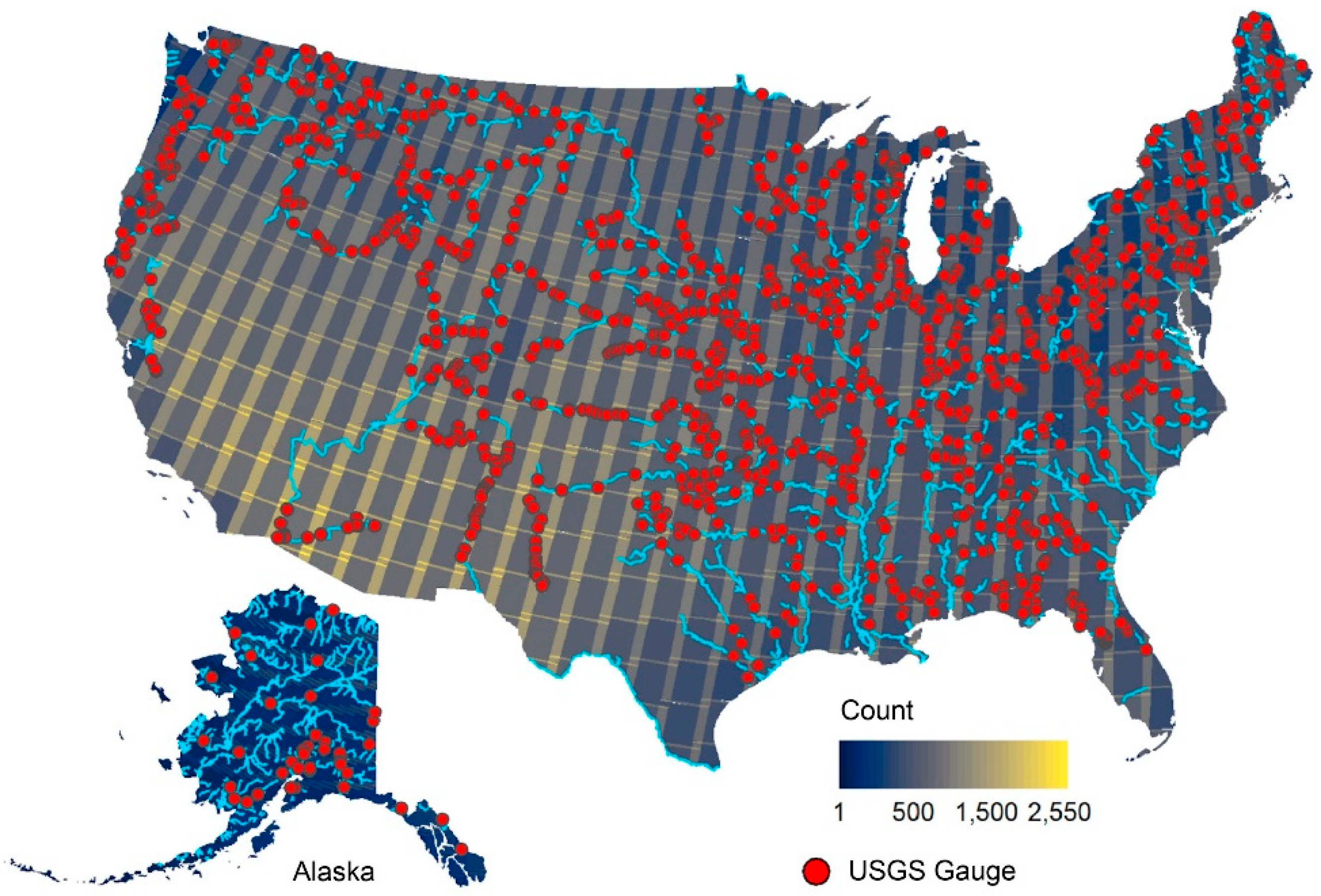
Map showing the United States Geological Survey (USGS) gauges used in this study and Landsat 5, 7, and 8 data availability based on the number of images with less than 30% cloud cover. Regions affected by cloud cover and low sun angle tend to have lower data availability. Rivers equal to or wider than Landsat’s 30 m resolution at mean discharge shown as blue lines [28].
Figure 1.
Map showing the United States Geological Survey (USGS) gauges used in this study and Landsat 5, 7, and 8 data availability based on the number of images with less than 30% cloud cover. Regions affected by cloud cover and low sun angle tend to have lower data availability. Rivers equal to or wider than Landsat’s 30 m resolution at mean discharge shown as blue lines [28].

Figure 2.
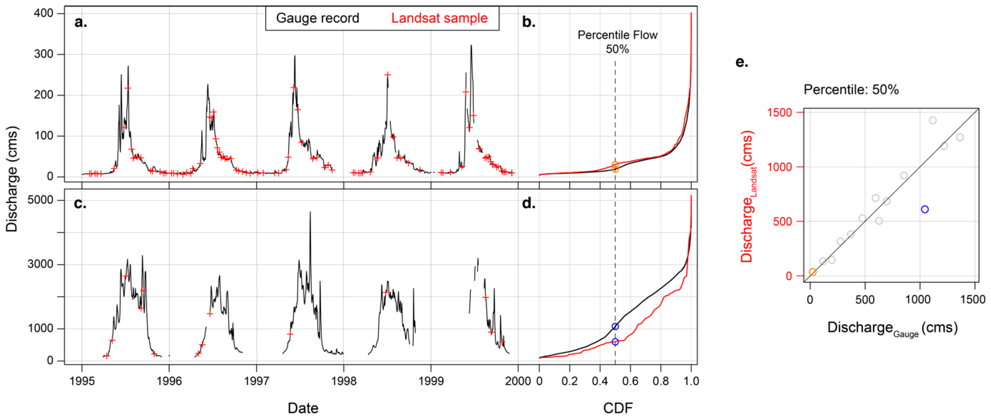
Hydrographs, cumulative density functions (CDFs), and a percentile plot from two example gauge stations. For visual clarity, hydrographs show a 5 year subset of the full record (1984–2019), while CDFs correspond to the full record length. Gaps in the hydrographs correspond to United States Geological Survey (USGS) flow observations that are estimated, provisional, and/or frozen. (a) Hydrograph of USGS Gauge 06225500 at Wind River near Crowheart, Wyoming, and (b) the corresponding flow frequency CDF (KSD statistic = 0.09, p-value < 0.001). (c) USGS Gauge 15129000 at Alsek River near Yakutat, Alaska, and (d) the corresponding flow frequency CDF (KSD statistic = 0.17, p-value = 0.055). (e) Fiftieth percentile (median) flow calculated from the full gauge record (x-axis) vs. from the Landsat sample (y-axis), with the two example gauge stations represented as colored circles. Gray circles represent median flows from other gauge stations.
Figure 2.
Hydrographs, cumulative density functions (CDFs), and a percentile plot from two example gauge stations. For visual clarity, hydrographs show a 5 year subset of the full record (1984–2019), while CDFs correspond to the full record length. Gaps in the hydrographs correspond to United States Geological Survey (USGS) flow observations that are estimated, provisional, and/or frozen. (a) Hydrograph of USGS Gauge 06225500 at Wind River near Crowheart, Wyoming, and (b) the corresponding flow frequency CDF (KSD statistic = 0.09, p-value < 0.001). (c) USGS Gauge 15129000 at Alsek River near Yakutat, Alaska, and (d) the corresponding flow frequency CDF (KSD statistic = 0.17, p-value = 0.055). (e) Fiftieth percentile (median) flow calculated from the full gauge record (x-axis) vs. from the Landsat sample (y-axis), with the two example gauge stations represented as colored circles. Gray circles represent median flows from other gauge stations.

Figure 3.
Individual gauge analysis, whereby each point represents metrics at a single gauge station. (a) Empirical CDF of the proportion of flow percentiles of the gauge record that the Landsat sample represents at each gauge. (b) Cloud occurrence correlates negatively with the ability of Landsat to capture flow frequency as represented by the KSD statistic. (c) Watershed area weakly correlates with the KSD statistic. (d) The Richards–Baker Flashiness Index does not correlate with the KSD statistic.

Figure 4.
Full gauge record flow percentiles vs. Landsat-sampled flow percentiles for each USGS gauge studied (N = 1134). The black line represents the 1:1 line and the red line represents the Theil–Sen median estimator best fit (equation shown in red). R2: coefficient of determination; rBias: relative bias; rRMSE: relative root mean square error; KSD: Kolmogorov–Smirnov D-statistic; MWW p: Mann–Whitney–Wilcoxon p-value.

Figure 5.
Landsat’s representation of flow conditions with increasing observation duration. (a) Variations in R2 value with increasing observation duration. (b) Relative metrics (rBias, rMAE, rRMSE) comparing gauge daily records and Landsat-sampled gauge records. (c) Absolute error metrics (Bias, MAE, RMSE, unit: cms) comparing gauge daily records and Landsat-sampled gauge records. Median statistical values plotted for each percentile.

© 2020 by the authors. Licensee MDPI, Basel, Switzerland. This article is an open access article distributed under the terms and conditions of the Creative Commons Attribution (CC BY) license (http://creativecommons.org/licenses/by/4.0/).
Share and Cite
MDPI and ACS Style
Allen, G.H.; Yang, X.; Gardner, J.; Holliman, J.; David, C.H.; Ross, M. Timing of Landsat Overpasses Effectively Captures Flow Conditions of Large Rivers. Remote Sens. 2020, 12, 1510. https://0-doi-org.brum.beds.ac.uk/10.3390/rs12091510
AMA Style
Allen GH, Yang X, Gardner J, Holliman J, David CH, Ross M. Timing of Landsat Overpasses Effectively Captures Flow Conditions of Large Rivers. Remote Sensing. 2020; 12(9):1510. https://0-doi-org.brum.beds.ac.uk/10.3390/rs12091510
Chicago/Turabian StyleAllen, George H., Xiao Yang, John Gardner, Joel Holliman, Cédric H. David, and Matthew Ross. 2020. "Timing of Landsat Overpasses Effectively Captures Flow Conditions of Large Rivers" Remote Sensing 12, no. 9: 1510. https://0-doi-org.brum.beds.ac.uk/10.3390/rs12091510
Note that from the first issue of 2016, this journal uses article numbers instead of page numbers. See further details here.