Effect of Image Fusion on Vegetation Index Quality—A Comparative Study from Gaofen-1, Gaofen-2, Gaofen-4, Landsat-8 OLI and MODIS Imagery

Abstract
:
1. Introduction
2. Materials and Methods
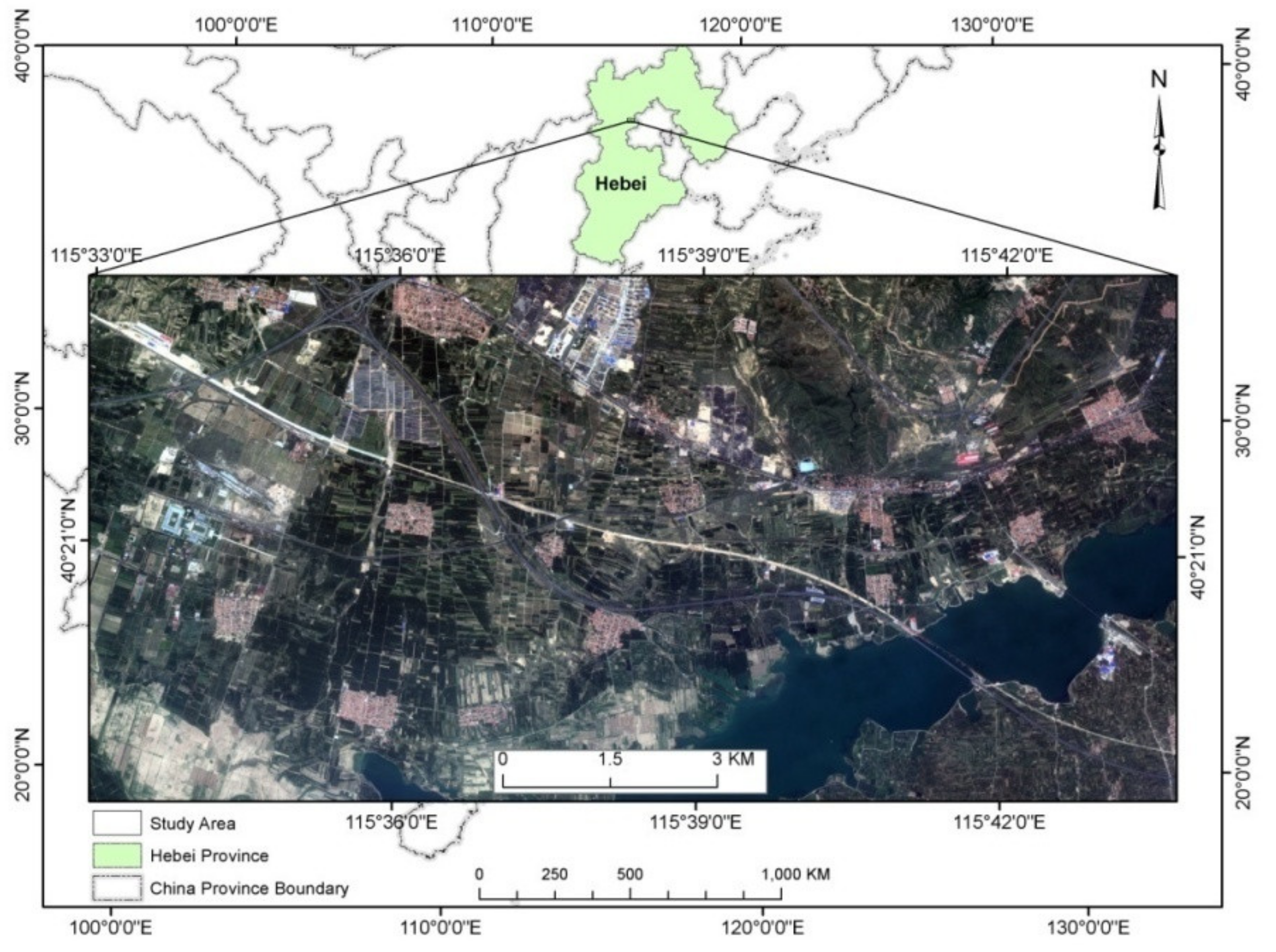
2.1. Study Area
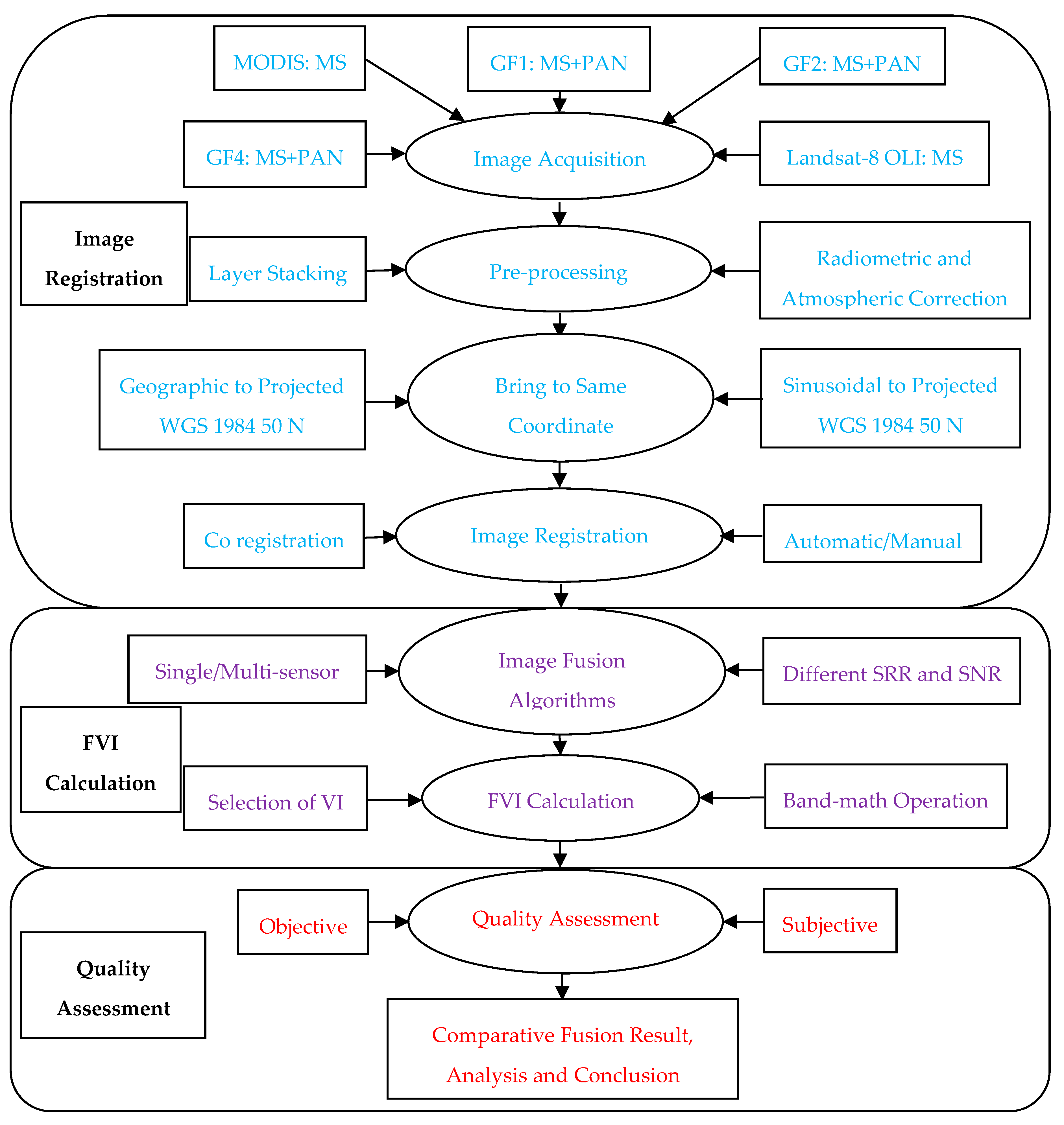
2.2. Methodology
2.2.1. Image Acquisition
2.2.2. Pre-processing
2.2.3. Same Coordinate System
2.2.4. Image Registration
2.2.5. Selection of Image Fusion Algorithms
2.2.6. Selection of VI
2.2.7. Strategy on Image Fusion and Quality Assessment
3. Results
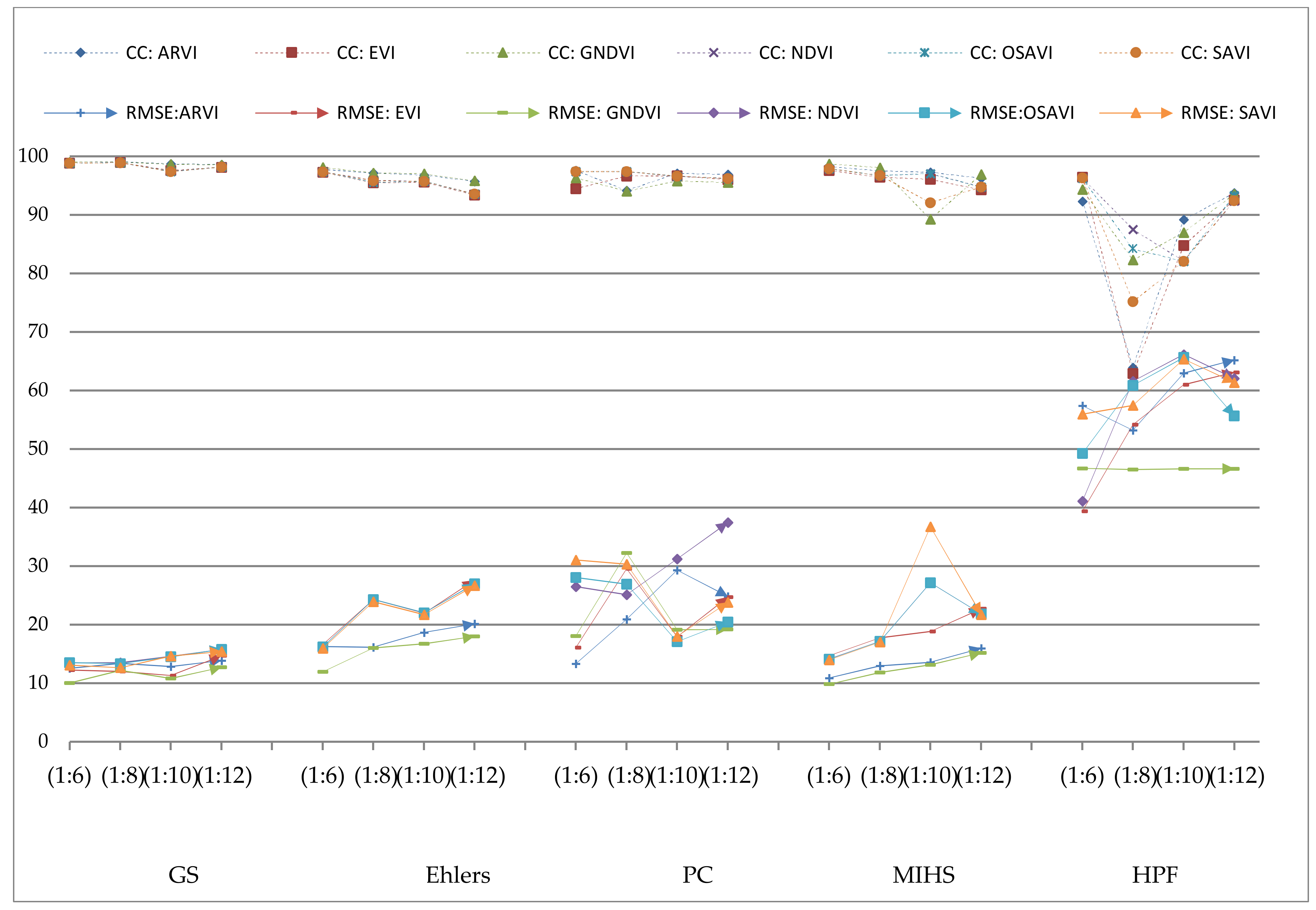
3.1. Single Sensor FVI Quality (Using Resampling)
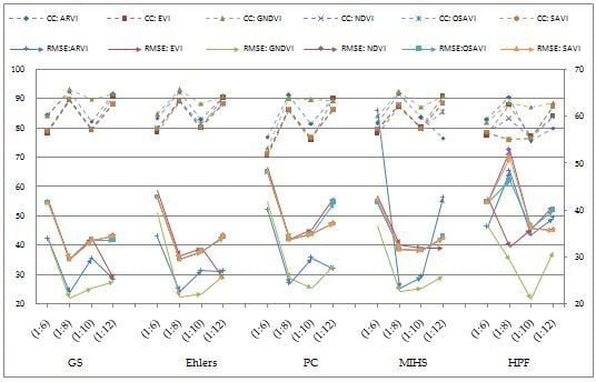
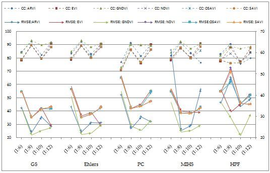
3.2. Multi-Sensor FVI Quality (Using Real Image)
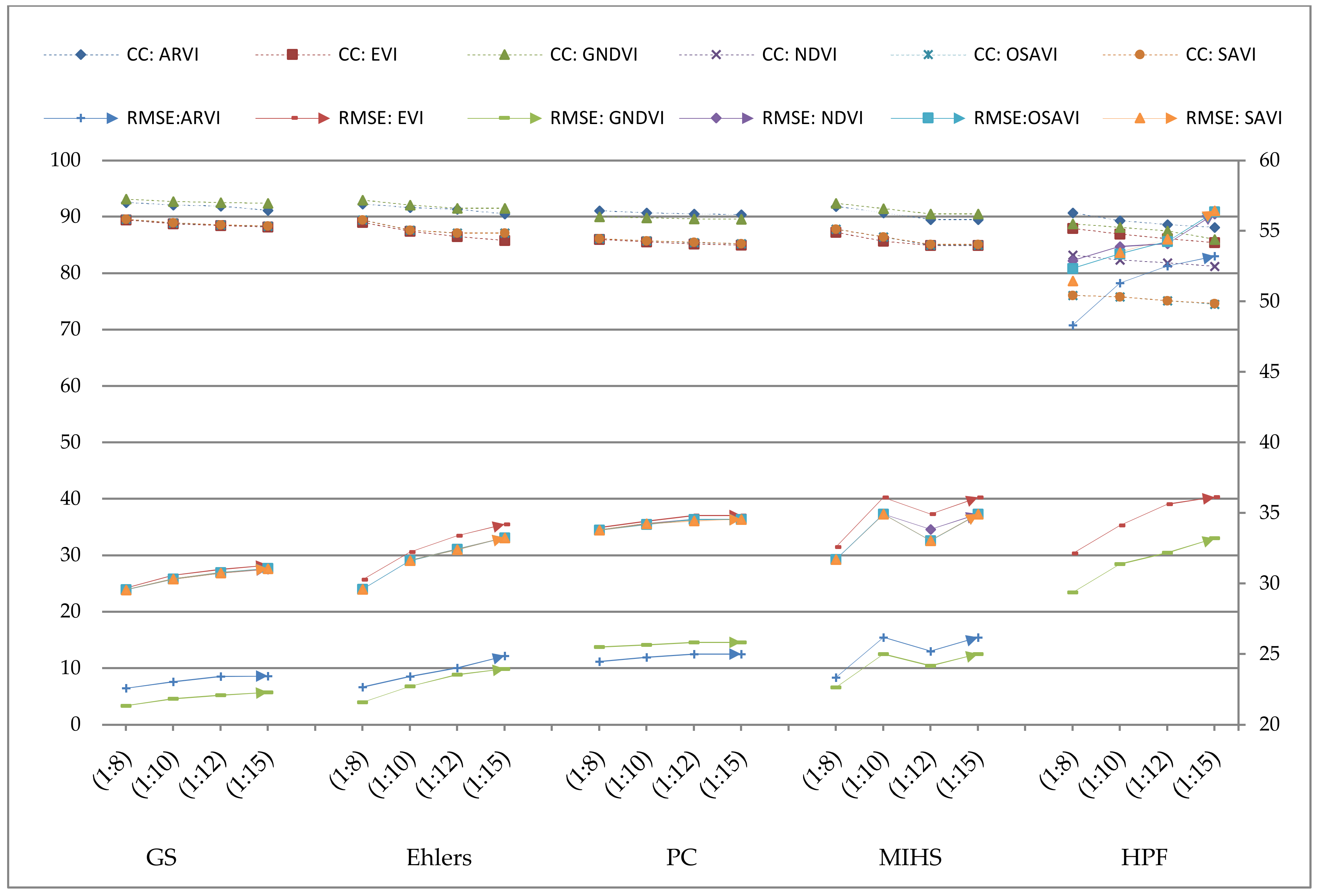
3.3. Multi-Sensor FVI Quality (Resampled)
3.4. Visual Quality Evaluation
4. Discussion
4.1. Quality Assessment
4.2. Influence of SRR (with Same SRF and Good SNR)
4.3. Influence of SRR (with different SRF and SNR (Good to Poor))
4.4. Influence of SRR (with constant SRF and Good SNR)
4.5. Limitations and Possible Future Study
5. Conclusions
Author Contributions
Funding
Acknowledgments
Conflicts of Interest
References
- El-mezouar, M.C.; Taleb, N.; Kpalma, K.; Ronsin, J. A high-resolution index for vegetation extraction in IKONOS images. In Proceedings of the SPIE on Remote Sensing for Agriculture, Ecosystems, and Hydrology, Toulouse, France, 22 October 2010; Volume 78242, pp. 1–9. [Google Scholar]
- Ehlers, M.; Klonus, S.; Astrand, P.J.; Rosso, P. Multi-sensor image fusion for pansharpening in remote sensing. Int. J. Image Data Fusion 2010, 1, 25–45. [Google Scholar] [CrossRef]
- Swathika, R.; Sharmila, T.S. Image fusion for MODIS and Landsat images using top hat based moving technique with FIS. Clust. Comput. 2019, 22, 12939–12947. [Google Scholar] [CrossRef]
- Jiang, D.; Zhuang, D.; Huang, Y. Investigation of Image Fusion for Remote Sensing Application. Available online: www.intechopen.com/books/new-advances-in-image-fusion/investigation-of-image-fusion-for-remote-sensing-application (accessed on 2 May 2020).
- Zeng, Y.; Zhang, J.; Genderen, J.L.; Zhang, Y. Image fusion for land cover change detection. Int. J. Image Data Fusion 2010, 1, 193–215. [Google Scholar] [CrossRef]
- Sarp, G. Spectral and spatial quality analysis of pan-sharpening algorithms: A case study in Istanbul. Eur. J. Remote Sens. 2014, 47, 19–28. [Google Scholar] [CrossRef] [Green Version]
- Sagan, V.; Maimaitijiang, M.; Sidike, P.; Maimaitiyiming, M.; Erkbol, H.; Hartling, S.; Peterson, K.T.; Peterson, J.; Burken, J.; Fritschi, F. Uav/satellite multiscale data fusion for crop monitoring and early stress detection. In Proceedings of the The International Archives of the Photogrammetry, Remote Sensing and Spatial Information Sciences, Enschede, The Netherlands, 10–14 June 2019; Volume XLII, pp. 715–722. [Google Scholar]
- Ghimire, P.; Deng, L. Image Fusion Technique: Algorithm to Application. Nepal. J. Geoinform. 2019, 18, 27–34. [Google Scholar]
- Gholinejad, S.; Fatemi, S.B. Optimum indices for vegetation cover change detection in the Zayandeh-rud river basin: A fusion approach. Int. J. Image Data Fusion 2019, 10, 199–216. [Google Scholar] [CrossRef]
- Roy, D.P.; Kovalskyy, V.; Zhang, H.K.; Vermote, E.F.; Yan, L.; Kumar, S.S.; Egorov, A. Characterization of Landsat-7 to Landsat-8 reflective wavelength and normalized difference vegetation index continuity. Remote Sens. Environ. 2016, 185, 57–70. [Google Scholar] [CrossRef] [Green Version]
- Xue, J.; Su, B. Significant Remote Sensing Vegetation Indices: A Review of Developments and Applications. J. Sens. 2017, 2017, 1–17. [Google Scholar] [CrossRef] [Green Version]
- Ahmad, F. Spectral vegetation indices performance evaluated for Cholistan Desert. J. Geogr. Reg. Plan. 2012, 5, 165–172. [Google Scholar]
- Johnson, B. Effects of pansharpening on vegetation indices. ISPRS Int. J. Geo-Inf. 2014, 3, 507–522. [Google Scholar] [CrossRef]
- Jagalingam, P.; Hegde, A.V. A Review of Quality Metrics for Fused Image. In Proceedings of the International Conference on Water Resources, Coastal and Ocean Engineering (ICWRCOE 2015), Mangalore, India, 12–14 March 2015; Elsevier: Amsterdam, The Netherlands, 2015; Volume 4, pp. 133–142. [Google Scholar]
- Zhu, X.X.; Bamler, R. A Sparse Image Fusion Algorithm With Application to Pan-Sharpening. IEEE Trans. Geosci. Remote Sens. 2013, 51, 2827–2836. [Google Scholar] [CrossRef]
- Liu, Y.; Chen, X.; Ward, R.K.; Wang, Z.J. Image Fusion With Convolutional Sparse Representation. IEEE Signal. Process. Lett. 2016, 23, 1882–1886. [Google Scholar] [CrossRef]
- Li, X.; Wang, L.; Cheng, Q.; Wu, P.; Gan, W.; Fang, L. Cloud removal in remote sensing images using nonnegative matrix factorization and error correction. ISPRS J. Photogramm. Remote Sens. 2019, 148, 103–113. [Google Scholar] [CrossRef]
- Li, X.; Shen, H.; Zhang, L.; Zhang, H.; Yuan, Q.; Yang, G. Recovering Quantitative Remote Sensing Products Contaminated by Thick Clouds and Shadows Using Multitemporal Dictionary Learning. IEEE Trans. Geosci. Remote Sens. 2014, 52, 7086–7098. [Google Scholar]
- Laben, C.A.; Brower, B.V. Process for Enhancing the Spatial Resolution of Multispectral Imagery using Pan-Sharpening. U.S. Patent 6011875, 4 January 2000. [Google Scholar]
- Klonus, S.; Ehlers, M. Performance of evaluation methods in image fusion. In Proceedings of the 12th International Conference on Information Fusion, Seattle, WA, USA, 6–9 July 2009; IEEE: Piscataway, NJ, USA, 2009; pp. 1409–1416. [Google Scholar]
- Klonus, S.; Ehlers, M. Image fusion using the Ehlers spectral characteristics preservation algorithm. Giscience Remote Sens. 2007, 44, 93–116. [Google Scholar] [CrossRef]
- Kang, T.; Zhang, X.; Wang, H. Assessment of the fused image of multispectral and panchromatic images of SPOT5 in the investigation of geological hazards. Sci. China Ser. E Technol. Sci. 2008, 51, 144–153. [Google Scholar] [CrossRef]
- Wu, J.; Jiang, P. A complete no-reference image quality assessment method based on local feature. Int. J. Image Data Fusion 2019, 10, 165–176. [Google Scholar] [CrossRef]
- Sahu, D.K.; Parsai, M.P. Different Image Fusion Techniques-A Critical Review. Int. J. Mod. Eng. Res. 2012, 2, 4298–4301. [Google Scholar]
- Jawak, S.D.; Luis, A.J. A Comprehensive Evaluation of PAN-Sharpening Algorithms Coupled with Resampling Methods for Image Synthesis of Very High Resolution Remotely Sensed Satellite Data. Adv. Remote Sens. 2013, 2, 332–344. [Google Scholar] [CrossRef] [Green Version]
- Nikolakopoulos, K.; Oikonomidis, D. Quality assessment of ten fusion techniques applied on Worldview-2. Eur. J. Remote Sens. 2015, 48, 141–167. [Google Scholar] [CrossRef]
- Sekrecka, A.; Kedzierski, M. Integration of Satellite Data with High Resolution Ratio: Improvement of Spectral Quality with Preserving Spatial Details. Sensors 2018, 18, 4418. [Google Scholar] [CrossRef] [PubMed] [Green Version]
- Ehlers, M. Multi-image Fusionin Remote Sensing: Spatial Enhancementvs. Spectral Characteristics Preservation. In Advances in Visual Computing, Proceedings of the 4th International Symposium, ISVC 2008,Part II, Las Vegas, NV, USA, 1–3 December 2008; Bebis, G., Parvin, B., Koracin, D., Boyle, R., Porikli, F., Peters, J., Klosowski, J., Rhyne, T.-M., Ams, L., Chun, Y.K., et al., Eds.; Springer: Berlin/Heidelberg, Germany, 2008; pp. 75–84. [Google Scholar]
- Ling, Y.; Ehlers, M.; Usery, E.L.; Madden, M. Effects of spatial resolution ratio in image fusion. Int. J. Remote Sens. 2008, 29, 2157–2167. [Google Scholar] [CrossRef]
- Zhou, J.; Civco, D.L.; Silander, J.A. A wavelet transform method to merge Landsat TM and SPOT panchromatic data. Int. J. Remote Sens. 1998, 19, 743–757. [Google Scholar] [CrossRef]
- Rahaman, K.R.; Hassan, Q.K.; Ahmed, M.R. Pan-Sharpening of Landsat-8 Images and Its Application in Calculating Vegetation Greenness and Canopy Water Contents. ISPRS Int. J. Geo-Inf. 2017, 6, 168. [Google Scholar] [CrossRef] [Green Version]
- Hwang, T.; Song, C.; Bolstad, P.V.; Band, L.E. Downscaling real-time vegetation dynamics by fusing multi-temporal MODIS and Landsat NDVI in topographically complex terrain. Remote Sens. Environ. 2011, 115, 2499–2512. [Google Scholar] [CrossRef]
- Hassan, Q.K.; Bourque, C.P.-A.; Meng, F.-R. Application of Landsat-7 ETM+ and MODIS products in mapping seasonal accumulation of growing degree days at an enhanced resolution. J. Appl. Remote Sens. 2007, 1, 013539. [Google Scholar] [CrossRef]
- Dao, P.D.; Mong, N.T.; Chan, H.-P. Landsat-MODIS image fusion and object-based image analysis for observing flood inundation in a heterogeneous vegetated scene. Giscience Remote Sens. 2019, 56, 1148–1169. [Google Scholar] [CrossRef]
- He, G.; Fang, H.; Bai, S.; Liu, X.; Chen, M.; Bai, J. Application of a three-dimensional eutrophication model for the Beijing Guanting Reservoir, China. Ecol. Model. 2011, 222, 1491–1501. [Google Scholar] [CrossRef]
- Wald, L.; Ranchin, T.; Mangolini, M. Fusion of satellite images of different spatial resolutions: Assessing the quality of resulting images. Photogramm. Eng. Remote Sens. 1997, 63, 691–699. [Google Scholar]
- Vermote, E.F.; Roger, J.C.; Ray, J.P. MODIS Surface Reflectance User’s Guide. Available online: https://lpdaac.usgs.gov/documents/306/MOD09_User_Guide_V6.pdf (accessed on 5 April 2020).
- Che, X.; Feng, M.; Sexton, J.O.; Channan, S.; Yang, Y.; Sun, Q. Assessment of MODIS BRDF/Albedo Model Parameters (MCD43A1 Collection 6) for Directional Reflectance Retrieval. Remote Sens. 2017, 9, 1123. [Google Scholar] [CrossRef] [Green Version]
- ENVI Atmospheric Correction Module: QUAC and FLAASH User’s Guide. Available online: http://www.harrisgeospatial.com/portals/0/pdfs/envi/flaash_module.pdf (accessed on 2 May 2020).
- Zhang, Z.; Han, D.; Dezert, J.; Yang, Y. A New Image Registration Algorithm Based on Evidential Reasoning. Sensors 2019, 19, 1091. [Google Scholar] [CrossRef] [PubMed] [Green Version]
- Feng, R.; Du, Q.; Li, X.; Shen, H. Robust registration for remote sensing images by combining and localizing feature- and area-based methods. ISPRS J. Photogramm. Remote Sens. 2019, 151, 15–26. [Google Scholar] [CrossRef]
- Murphy, J.M.; Moigne, J.; Le Harding, D.J.; Space, G. Automatic Image Registration of Multi-Modal Remotely Sensed Data with Global Shearlet Features. IEEE Trans. Geosci. Remote Sens. 2017, 54, 1685–1704. [Google Scholar] [CrossRef] [PubMed] [Green Version]
- Jin, X. ENVI Automated Image Registration Solutions. Available online: https://www.harrisgeospatial.com/portals/0/pdfs/ENVI_Image_Registration_Whitepaper.pdf (accessed on 5 April 2020).
- Kaufman, Y.J.; Tanre, D. Atmospherically Resistant Vegetation Index (ARVI) for EOS-MODIS. IEEE Trans. Geosci. Remote Sens. 1992, 30, 260–271. [Google Scholar] [CrossRef]
- Huete, A.; Didan, K.; Miura, T.; Rodriguez, E.P.; Gao, X.; Ferreira, L.G. Overview of the radiometric and biophysical performance of the MODIS vegetation indices. Remote Sens. Environ. 2002, 83, 195–213. [Google Scholar] [CrossRef]
- Gitelson, A.A.; Kaufman, Y.J.; Merzlyak, M.N. Use of a Green Channel in Remote Sensing of Global Vegetation from EOS-MODIS. Remote Sens. Environ. 1996, 58, 289–298. [Google Scholar] [CrossRef]
- Cheng, W.-C.; Chang, J.-C.; Chang, C.-P.; Su, Y.; Tu, T.-M. A Fixed-Threshold Approach to Generate High-Resolution Vegetation Maps for IKONOS Imagery. Sensors 2008, 8, 4308–4317. [Google Scholar] [CrossRef]
- Aiazzi, B.; Alparone, L.; Baronti, S.; Garzelli, A. Context-Driven Fusion of High Spatial and Spectral Resolution Images Based on Oversampled Multiresolution Analysis. IEEE Trans. Geosci. Remote Sens. 2002, 40, 2300–2312. [Google Scholar] [CrossRef]
- Huete, A.R. A Soil-Adjusted Vegetation Index (SAVI). Remote Sens. Environ. 1988, 25, 295–309. [Google Scholar] [CrossRef]
- Budhewar, S.T. Wavelet and Curvelet Transform based Image Fusion Algorithm. Int. J. Comput. Sci. Inf. Technol. 2014, 5, 3703–3707. [Google Scholar]
- Gamba, P. Image and data fusion in remote sensing of urban areas: Status issues and research trends. Int. J. Image Data Fusion 2014, 5, 2–12. [Google Scholar] [CrossRef]
- Ren, J.; Yang, W.; Yang, X.; Deng, X.; Zhao, H.; Wang, F.; Wang, L. Optimization of Fusion Method for GF-2 Satellite Remote Sensing Images based on the Classification Effect. Earth Sci. Res. J. 2019, 23, 163–169. [Google Scholar] [CrossRef]
- Pandit, V.R.; Bhiwani, R.J. Image Fusion in Remote Sensing Applications: A Review. Int. J. Comput. Appl. 2015, 120, 22–32. [Google Scholar]
- Fonseca, L.; Namikawa, L.; Castejon, E.; Carvalho, L.; Pinho, C.; Pagamisse, A. Image Fusion for Remote Sensing Applications. Available online: http://www.intechopen.com/books/image-fusion-and-its-applications/image-fusion-for-remote-sensing-applications (accessed on 2 May 2020).
- Vibhute, A.D.; Dhumal, R.; Nagne, A.; Gaikwad, S.; Kale, K.V.; Mehrotra, S.C. Multi-Sensor, Multi-Resolution and Multi-Temporal Satellite Data Fusion for Soil Type Classification. In Proceedings of the International Conference on Cognitive Knowledge Engineering, Aurangabad, India, 21–23 December 2016; pp. 27–32. [Google Scholar]
- Belgiu, M.; Stein, A. Spatiotemporal Image Fusion in Remote Sensing. Remote Sens. 2019, 11, 818. [Google Scholar] [CrossRef] [Green Version]
- Al-Wassai, F.A.; Kalyankar, N.V.; Al-Zaky, A.A. Spatial and Spectral Quality Evaluation Based on Edges Regions of Satellite Image fusion. In Proceedings of the 2012 Second International Conference on Advanced Computing and Communication Technologies (ACCT), Haryana, India, 7–8 January 2012; IEEE: Piscataway, NJ, USA, 2012; pp. 265–275. [Google Scholar]
- Zhang, D.; Xie, F.; Zhang, L. Preprocessing and fusion analysis of GF-2 satellite Remote-sensed spatial data. In Proceedings of the 2018 International Conference on Information Systems and Computer Aided Education (ICISCAE), Changchun, China, 6–8 July 2018; IEEE: Piscataway, NJ, USA, 2018; pp. 24–29. [Google Scholar]
- Sun, W.; Chen, B.; Messinger, D.W. Nearest-neighbor diffusion-based pan-sharpening algorithm for spectral images. Opt. Eng. 2014, 53, 013107. [Google Scholar] [CrossRef] [Green Version]
- Wang, Z.; Bovik, A.C.; Sheikh, H.R.; Simoncelli, E.P. Image Quality Assessment: From Error Visibility to Structural Similarity. IEEE Trans. Image Process. 2004, 13, 600–612. [Google Scholar] [CrossRef] [Green Version]


| Collection Date | Satellite Images | Resolution | Imager Type | Available Bands | Selected Bands for This Research |
|---|---|---|---|---|---|
| 2017/07/13 | Gaofen-1 | PAN-2 m, MS-8 m | Pushbroom with TDI capability | 4 | B1/blue 0.45-0.52 µm B2/green 0.52-0.59 µm B3/red 0.63-0.69 µm B4/NIR 0.77-0.89 µm PAN 0.45-0.90 µm |
| Gaofen-2 | PAN-1 m, MS-4 m | ||||
| Gaofen-4 | PAN-50 m, MS-50 m | ||||
| 2017/07/17 | Landsat-8 OLI | MS-30 m | Operational Land Imager (OLI) | 11 | B1/blue 0.45-0.51 µm B2/green 0.53-0.59 µm B3/red 0.64-0.67 µm B4/NIR 0.85-0.88 µm |
| 2017/07/13 | MODIS | MS-500 m | MODIS Payload Imaging Sensor | 7 | B3/blue 0.45-0.47 µm B4/green 0.54-0.56µm B1/red 0.62-0.67 µm B2/NIR 0.84-0.87 µm |
| Algorithms | Details | Advantages | References |
|---|---|---|---|
| GS | A generalization of PCA, in which PC1 may be arbitrarily chosen and the remaining components are calculated to be orthogonal or uncorrelated to one another. | Spectral characteristics of lower-spatial-resolution MS data are preserved. | [6,19,20] |
| Ehlers | Enhances high-frequency changes such as edges and grey level discontinuities in an image. | Spectral characteristic preserving. | [21] |
| PC | Replacement of PC1 by high-resolution image, which contains the most information of the image resembles. | Gives high-resolution MS images. | [6,22,23,24] |
| MIHS | Making forward PCA transform for both intensity component(I) and high-resolution panchromatic images getting the first component as I‘. Matching the histogram of I’ component with I to make I’’ and finally transferring I’’, H, S to RGB true color space. | Involves both HIS and PCA methods, Preserves both spatial and spectral details. | [25,26] |
| HPF | High-frequency spatial content of the pan image is extracted using a high-pass filter and transferred to the resampled MS image. | Preserves a high percentage of the spectral characteristics of the MS image. | [22,23] |
| VIs | Characteristics | Definition | References |
|---|---|---|---|
| ARVI | The improvement is much better for vegetated surfaces than for soils. | (NIR-2*R-B)/(NIR+2*R-B) | [44] |
| EVI | Estimates vegetation LAI, biomass and water content, and improve sensitivity in high biomass region. | 2.5*[(NIR-R)/(NIR+6*R-7.5*B+1)] | [45] |
| GNDVI | Has a wider dynamic range than the NDVI and is, on average, at least five times more sensitive to chlorophyll concentration. | (NIR-G)/(NIR+G) | [44,46] |
| NDVI | Detects change in the amount of green biomass efficiently in vegetation with low to moderate density. | (NIR-R)/(NIR+R) | [9,11,12,13,47] |
| OSAVI | OSAVI does not depend on the soil line and can eliminate the influence of the soil background effectively. Where L is around 0.16. | (L+1)*[(NIR-R)/(NIR+R+L+1) | [11,48] |
| SAVI | Minimizes soil brightness influences from spectral vegetation indices involving red and near-infrared (NIR) wavelengths. Where L is around 0.5. | (L+1)*[(NIR-R)/(NIR+R+L+1) | [22,49] |
| SRR | Fusion Type | Original Resolution | Resampled Resolution | Activity/ Computation | Quality Indices |
|---|---|---|---|---|---|
| 1:6 | Same-Sensor (GF2+GF2) | GF2 (PAN-1 m) GF2 (MS-4 m) | GF2 (MS-1 m) GF2 (MS-6 m) | 1. Compute 1 m RVI and 1 m FVI 2. Assess RVI and FVI | |
| Multi-Sensor (GF1+GF4) | GF1(PAN-2 m) GF1(MS-8 m) GF4( MS-50 m) | GF1(PAN-8 m) GF4( MS-50 m) | 1. Compute 8 m RVI and 8 m FVI 2. Assess RVI and FVI | ||
| 1:8 | Same-Sensor (GF2+GF2) | GF2 (PAN-1 m) GF2 (MS-4 m) | GF2 (MS-1 m) GF2 (MS-8 m) | 1. Compute 1 m RVI and 1 m FVI 2. Assess RVI and FVI | |
| Multi-Sensor (GF2+Landsat-8 OLI) | GF2 (PAN-1 m) GF2 (MS-4 m) LS-8 (MS-30 m) | GF2 (PAN-4 m) | 1. Compute 4 m RVI and 4 m FVI 2. Assess RVI and FVI | ||
| 1:10 | Same-Sensor (GF2+GF2) | GF2 (PAN-1 m) GF2 (MS-4 m) | GF2 (MS-1 m) GF2 (MS-10 m) | 1. Compute 1 m RVI and 1 m FVI 2. Assess RVI and FVI | 1.Objective (CC, RMSE) |
| Multi-Sensor (GF4+MODIS) | GF4 (PAN-50 m) GF4 (MS-50 m) MODIS (MS-500 m) | -- | 1. Compute 50 m RVI and 50 m FVI 2. Assess RVI and FVI | ||
| Multi-Sensor (GF2+Landsat-8 OLI) | GF2 (PAN-1 m) GF1(MS-4 m) LS-8( MS-30 m) | GF1(PAN-4 m) LS-8 (MS-40 m) | 1. Compute 4 m RVI and 4 m FVI 2. Assess RVI and FVI | ||
| 1:12 | Same-Sensor (GF2+GF2) | GF2 (PAN-1 m) GF2 (MS-4 m) | GF2 (MS-1 m) GF2 (MS-12 m) | 1. Compute 1 m RVI and 1 m FVI 2. Assess RVI and FVI | 2.Subjective (Visual Inspection) |
| Multi-Sensor (GF2+GF4) | GF2 (PAN-1 m) GF2 (MS-4 m) GF4( MS-50 m) | GF2 (PAN-4 m) | 1. Compute 4 m RVI and 4 m FVI 2. Assess RVI and FVI | ||
| Multi-Sensor (GF2+Landsat-8 OLI) | GF2 (PAN-1 m) GF1(MS-4 m) LS-8( MS-30 m) | GF2(PAN-4 m) LS-8 (MS-48 m) | 1. Compute 4 m RVI and 4 m FVI 2. Assess RVI and FVI |
| SRR | Indices (%) | Image Fusion | ARVI | EVI | GNDVI | NDVI | OSAVI | SAVI |
|---|---|---|---|---|---|---|---|---|
| 1:6 GF2+GF2 | CC | GS | 99.05 | 98.85 | 99.03 | 98.86 | 98.87 | 98.86 |
| Ehlers | 97.76 | 97.32 | 98.13 | 97.36 | 97.37 | 97.36 | ||
| PC | 97.62 | 94.47 | 96.34 | 97.39 | 97.40 | 97.40 | ||
| MIHS | 98.28 | 97.62 | 98.73 | 97.88 | 97.89 | 97.91 | ||
| HPF | 92.35 | 96.46 | 94.36 | 96.28 | 96.29 | 96.33 | ||
| RMSE | GS | 12.58 | 12.26 | 10.06 | 13.48 | 13.50 | 13.11 | |
| Ehlers | 16.30 | 16.65 | 11.96 | 16.19 | 16.19 | 16.00 | ||
| PC | 13.36 | 16.10 | 18.08 | 26.51 | 28.05 | 31.09 | ||
| MIHS | 10.90 | 14.75 | 9.85 | 14.16 | 14.14 | 14.00 | ||
| HPF | 57.43 | 39.39 | 46.71 | 41.13 | 49.30 | 55.96 | ||
| 1:8 GF2+GF2 | CC | GS | 99.08 | 98.94 | 99.04 | 98.93 | 98.94 | 98.93 |
| Ehlers | 97.15 | 95.48 | 97.18 | 95.93 | 95.53 | 95.83 | ||
| PC | 94.16 | 96.61 | 94.04 | 97.41 | 97.41 | 97.42 | ||
| MIHS | 97.56 | 96.44 | 98.05 | 96.77 | 96.77 | 96.78 | ||
| HPF | 63.97 | 62.91 | 82.30 | 87.53 | 84.20 | 75.19 | ||
| RMSE | GS | 13.40 | 12.00 | 12.19 | 13.54 | 13.35 | 12.66 | |
| Ehlers | 16.14 | 24.30 | 16.02 | 24.30 | 24.30 | 23.97 | ||
| PC | 40.94 | 29.58 | 32.28 | 25.16 | 26.93 | 30.33 | ||
| MIHS | 12.97 | 17.76 | 11.86 | 17.17 | 17.17 | 17.06 | ||
| HPF | 53.22 | 54.16 | 46.54 | 61.62 | 60.91 | 37.50 | ||
| 1:10 GF2+GF2 | CC | GS | 98.73 | 97.57 | 98.68 | 97.50 | 97.39 | 97.40 |
| Ehlers | 96.81 | 95.59 | 97.04 | 95.72 | 95.72 | 95.72 | ||
| PC | 97.13 | 96.68 | 95.8 | 96.60 | 96.61 | 96.61 | ||
| MIHS | 97.31 | 96.07 | 89.26 | 97.04 | 97.04 | 92.11 | ||
| HPF | 89.22 | 84.77 | 86.99 | 82.11 | 82.10 | 82.11 | ||
| RMSE | GS | 12.88 | 11.33 | 10.81 | 14.60 | 14.56 | 14.66 | |
| Ehlers | 18.68 | 21.98 | 16.73 | 22.00 | 22.21 | 21.75 | ||
| PC | 29.34 | 17.97 | 19.13 | 31.22 | 17.12 | 18.11 | ||
| MIHS | 13.60 | 18.84 | 13.17 | 27.15 | 27.15 | 36.74 | ||
| HPF | 63.00 | 61.12 | 46.65 | 66.17 | 65.65 | 65.38 | ||
| 1:12 GF2+GF2 | CC | GS | 98.59 | 98.15 | 98.53 | 98.17 | 98.17 | 98.17 |
| Ehlers | 95.72 | 93.41 | 95.88 | 93.57 | 93.57 | 93.57 | ||
| PC | 96.95 | 96.06 | 95.58 | 96.25 | 96.24 | 96.20 | ||
| MIHS | 96.29 | 94.29 | 96.91 | 94.78 | 94.78 | 94.78 | ||
| HPF | 93.76 | 92.55 | 93.57 | 92.36 | 93.37 | 92.43 | ||
| RMSE | GS | 13.86 | 14.70 | 12.77 | 15.78 | 15.78 | 15.43 | |
| Ehlers | 20.19 | 27.60 | 18.04 | 26.98 | 26.98 | 26.70 | ||
| PC | 14.85 | 24.70 | 19.24 | 47.47 | 20.45 | 23.85 | ||
| MIHS | 15.97 | 22.72 | 15.20 | 21.82 | 21.82 | 21.73 | ||
| HPF | 74.74 | 71.27 | 26.65 | 26.17 | 25.65 | 25.38 |
| SRR | Indices (%) | Image Fusion | ARVI | EVI | GNDVI | NDVI | OSAVI | SAVI |
|---|---|---|---|---|---|---|---|---|
| 1:6 (GF1+GF4) | CC | GS | 84.27 | 78.21 | 84.24 | 78.93 | 78.93 | 78.92 |
| Ehlers | 83.34 | 78.54 | 84.65 | 79.72 | 79.72 | 79.70 | ||
| PC | 77.00 | 70.47 | 73.21 | 71.04 | 71.04 | 71.04 | ||
| MIHS | 81.76 | 78.16 | 84.19 | 79.55 | 79.55 | 79.55 | ||
| HPF | 82.80 | 77.55 | 81.84 | 78.47 | 78.47 | 78.47 | ||
| RMSE | GS | 33.97 | 42.07 | 33.60 | 41.69 | 41.68 | 41.68 | |
| Ehlers | 34.42 | 44.23 | 39.47 | 42.79 | 42.79 | 42.79 | ||
| PC | 40.16 | 49.22 | 41.92 | 48.21 | 48.21 | 48.21 | ||
| MIHS | 61.33 | 43.06 | 36.61 | 41.77 | 41.79 | 42.52 | ||
| HPF | 36.59 | 42.97 | 36.62 | 41.73 | 41.74 | 41.74 | ||
| 1:8 (GF2+Landsat-8) | CC | GS | 92.56 | 89.45 | 93.13 | 89.57 | 89.57 | 89.57 |
| Ehlers | 92.26 | 89.02 | 92.98 | 89.44 | 89.44 | 89.44 | ||
| PC | 91.08 | 85.99 | 90.00 | 86.15 | 86.15 | 86.15 | ||
| MIHS | 91.82 | 87.23 | 92.38 | 87.81 | 87.82 | 87.82 | ||
| HPF | 90.69 | 87.97 | 88.78 | 83.23 | 76.06 | 76.08 | ||
| RMSE | GS | 22.59 | 29.69 | 21.35 | 29.57 | 29.57 | 29.56 | |
| Ehlers | 22.68 | 30.28 | 21.59 | 29.61 | 29.60 | 29.60 | ||
| PC | 24.47 | 33.97 | 25.51 | 33.81 | 33.81 | 33.81 | ||
| MIHS | 23.36 | 32.59 | 22.64 | 31.71 | 31.71 | 31.71 | ||
| HPF | 48.32 | 32.13 | 29.39 | 52.88 | 46.33 | 51.47 | ||
| 1:10 (GF4+MODIS) | CC | GS | 82.20 | 79.29 | 89.93 | 79.47 | 79.50 | 79.46 |
| Ehlers | 82.86 | 80.00 | 88.35 | 80.13 | 81.40 | 80.14 | ||
| PC | 81.56 | 75.84 | 89.68 | 76.45 | 76.64 | 76.77 | ||
| MIHS | 83.71 | 80.17 | 87.13 | 79.83 | 79.84 | 79.81 | ||
| HPF | 75.57 | 77.12 | 87.26 | 76.64 | 76.65 | 76.65 | ||
| RMSE | GS | 28.94 | 33.76 | 22.86 | 33.35 | 33.36 | 33.00 | |
| Ehlers | 28.35 | 33.07 | 24.34 | 32.69 | 31.68 | 31.65 | ||
| PC | 29.26 | 35.98 | 23.14 | 35.40 | 35.14 | 35.30 | ||
| MIHS | 27.72 | 33.27 | 25.43 | 33.20 | 33.21 | 33.21 | ||
| HPF | 35.11 | 35.83 | 25.33 | 36.12 | 36.12 | 36.11 | ||
| 1:12 (GF2+GF4) | CC | GS | 91.59 | 90.91 | 91.75 | 88.23 | 88.25 | 88.24 |
| Ehlers | 90.44 | 90.51 | 90.78 | 88.27 | 88.26 | 88.27 | ||
| PC | 90.00 | 90.21 | 89.21 | 86.24 | 86.22 | 86.24 | ||
| MIHS | 76.65 | 90.75 | 90.88 | 88.61 | 85.57 | 88.62 | ||
| HPF | 79.95 | 84.18 | 88.68 | 87.40 | 83.81 | 87.40 | ||
| RMSE | GS | 25.25 | 25.23 | 24.86 | 34.67 | 33.66 | 34.67 | |
| Ehlers | 27.09 | 25.23 | 26.32 | 34.67 | 34.34 | 34.66 | ||
| PC | 27.58 | 42.77 | 28.44 | 37.33 | 41.76 | 37.32 | ||
| MIHS | 42.77 | 31.94 | 26.10 | 34.18 | 34.39 | 34.18 | ||
| HPF | 38.41 | 40.94 | 31.38 | 35.83 | 40.12 | 35.83 |
| SRR | Indices (%) | Image Fusion | ARVI | EVI | GNDVI | NDVI | OSAVI | SAVI |
|---|---|---|---|---|---|---|---|---|
| 1:10 (GF2+Landsat-8 (40 m)) | CC | GS | 92.11 | 88.77 | 92.73 | 88.93 | 88.92 | 88.93 |
| Ehlers | 91.65 | 87.46 | 92.12 | 87.65 | 87.66 | 87.65 | ||
| PC | 90.74 | 85.58 | 89.81 | 85.76 | 85.76 | 85.77 | ||
| MIHS | 90.72 | 85.70 | 91.47 | 86.44 | 86.42 | 86.42 | ||
| HPF | 89.33 | 86.93 | 88.12 | 82.33 | 75.83 | 75.85 | ||
| RMSE | GS | 23.05 | 30.58 | 21.84 | 30.34 | 30.33 | 30.32 | |
| Ehlers | 23.42 | 32.24 | 22.72 | 31.65 | 31.63 | 31.65 | ||
| PC | 24.79 | 34.43 | 25.65 | 34.26 | 34.21 | 34.26 | ||
| MIHS | 26.18 | 36.12 | 25.01 | 34.94 | 34.93 | 34.93 | ||
| HPF | 51.32 | 34.13 | 31.39 | 53.89 | 53.36 | 53.47 | ||
| 1:12 (GF2+Landsat-8 (48 m)) | CC | GS | 91.88 | 88.43 | 92.54 | 88.60 | 88.59 | 88.60 |
| Ehlers | 91.34 | 86.52 | 91.52 | 87.15 | 87.15 | 87.16 | ||
| PC | 90.54 | 85.21 | 89.65 | 85.44 | 85.43 | 85.47 | ||
| MIHS | 89.54 | 84.92 | 90.52 | 85.00 | 85.00 | 85.11 | ||
| HPF | 88.63 | 86.13 | 87.52 | 81.83 | 75.13 | 75.15 | ||
| RMSE | GS | 23.43 | 31.02 | 22.10 | 30.75 | 30.79 | 30.75 | |
| Ehlers | 24.03 | 33.40 | 23.55 | 32.45 | 32.45 | 32.43 | ||
| PC | 25.00 | 34.82 | 25.84 | 34.55 | 34.55 | 34.44 | ||
| MIHS | 25.20 | 34.93 | 24.17 | 33.84 | 33.04 | 33.05 | ||
| HPF | 52.52 | 35.63 | 32.19 | 54.09 | 54.26 | 54.42 | ||
| 1:15 (GF2+Landsat-8 (60 m)) | CC | GS | 91.17 | 88.19 | 92.40 | 88.36 | 88.35 | 88.36 |
| Ehlers | 90.55 | 85.79 | 91.52 | 87.15 | 87.15 | 87.16 | ||
| PC | 90.42 | 84.98 | 89.55 | 85.25 | 85.24 | 85.24 | ||
| MIHS | 89.54 | 84.92 | 90.52 | 85.00 | 85.00 | 85.11 | ||
| HPF | 88.14 | 85.43 | 86.02 | 81.24 | 74.53 | 74.65 | ||
| RMSE | GS | 23.45 | 31.32 | 22.30 | 31.04 | 31.08 | 31.05 | |
| Ehlers | 24.87 | 34.21 | 23.96 | 33.24 | 33.24 | 33.25 | ||
| PC | 25.00 | 34.82 | 25.84 | 34.55 | 34.55 | 34.56 | ||
| MIHS | 26.18 | 36.12 | 25.01 | 34.94 | 34.93 | 34.92 | ||
| HPF | 53.21 | 36.13 | 33.21 | 56.21 | 56.36 | 56.43 |
| RVI and Fusion Algorithms | Same-Sen. ARVI(1 m) | Multi-Sen. EVI(8 m) | Same-Sen. NDVI(1 m) | Multi-Sen. GNDVI(8 m) | Same-Sen. OSAVI(1 m) | Multi-Sen. SAVI(8 m) |
|---|---|---|---|---|---|---|
| RVI (1 m, 8 m) |  |  |  |  |  |  |
| GS (1:6) |  |  |  |  |  |  |
| Ehlers (1:6) |  |  |  |  |  |  |
| PC ( 1:6) |  |  |  |  |  |  |
| MIHS (1:6) |  |  |  |  |  |  |
| HPF (1:6) |  |  |  |  |  |  |
| RVI and Fusion Algorithms | Same-Sen. ARVI(1 m) | Multi-Sen. EVI(4 m) | Same-Sen. NDVI(1 m) | Multi-Sen. GNDVI(4 m) | Same-Sen. OSAVI(1 m) | Multi-Sen. SAVI(4 m) |
| RVI (1 m, 4 m) |  |  |  |  |  |  |
| GS (1:8) |  |  |  |  |  |  |
| Ehlers (1:8) |  |  |  |  |  |  |
| PC ( 1:8) |  |  |  |  |  |  |
| MIHS (1:8) |  |  |  |  |  |  |
| HPF (1:8) |  |  |  |  |  |  |
| RVI and Fusion Algorithms | Same-Sen. ARVI(1 m) | Multi-Sen. EVI(50 m) | Multi-Sen(R) NDVI(4 m) | Same-Sen. GNDVI(1 m) | Multi-Sen. OSAVI(50 m) | Multi-Sen(R) SAVI(4 m) |
| RVI (1, 50, 4 m) |  |  |  |  |  |  |
| GS (1:10) |  |  |  |  |  |  |
| Ehlers (1:10) |  |  |  |  |  |  |
| PC ( 1:10) |  |  |  |  |  |  |
| MIHS (1:10) |  |  |  |  |  |  |
| HPF (1:10) |  |  |  |  |  |  |
| RVI and Fusion Algorithms | Same-Sen. ARVI(1 m) | Multi-Sen. EVI(4 m) | Multi-Sen(R) NDVI(4 m) | Same-Sen. GNDVI(1 m) | Multi-Sen. OSAVI(4 m) | Multi-Sen(R) SAVI(4 m) |
| RVI (1 m, 4 m) |  |  |  |  |  |  |
| GS (1:12) |  |  |  |  |  |  |
| Ehlers (1:12) |  |  |  |  |  |  |
| PC ( 1:12) |  |  |  |  |  |  |
| MIHS (1:12) |  |  |  |  |  |  |
| HPF (1:12) |  |  |  |  |  |  |
© 2020 by the authors. Licensee MDPI, Basel, Switzerland. This article is an open access article distributed under the terms and conditions of the Creative Commons Attribution (CC BY) license (http://creativecommons.org/licenses/by/4.0/).
Share and Cite
Ghimire, P.; Lei, D.; Juan, N. Effect of Image Fusion on Vegetation Index Quality—A Comparative Study from Gaofen-1, Gaofen-2, Gaofen-4, Landsat-8 OLI and MODIS Imagery. Remote Sens. 2020, 12, 1550. https://0-doi-org.brum.beds.ac.uk/10.3390/rs12101550
Ghimire P, Lei D, Juan N. Effect of Image Fusion on Vegetation Index Quality—A Comparative Study from Gaofen-1, Gaofen-2, Gaofen-4, Landsat-8 OLI and MODIS Imagery. Remote Sensing. 2020; 12(10):1550. https://0-doi-org.brum.beds.ac.uk/10.3390/rs12101550
Chicago/Turabian StyleGhimire, Prakash, Deng Lei, and Nie Juan. 2020. "Effect of Image Fusion on Vegetation Index Quality—A Comparative Study from Gaofen-1, Gaofen-2, Gaofen-4, Landsat-8 OLI and MODIS Imagery" Remote Sensing 12, no. 10: 1550. https://0-doi-org.brum.beds.ac.uk/10.3390/rs12101550