The Local Median Filtering Method for Correcting the Laser Return Intensity Information from Discrete Airborne Laser Scanning Data

Abstract

Laser return intensity (LRI) information obtained from airborne laser scanning (ALS) data has been used to classify land cover types and to reveal canopy physiological features. However, the sensor-related and environmental parameters may introduce noise. In this study, we developed a local median filtering (LMF) method to point-by-point correct the LRI information. For each point, we deduced the reference variation range for its LRI. Then, we replaced the outliers of LRI with their local median values. To evaluate the LMF method, we assessed the discrepancy of LRI information from the same and diverse land cover types. Moreover, we used the corrected LRI to distinguish points from grass, road, and bare land, which were classified as ground type in ALS data. The results show that using the LMF method could increase the similarity of pointwise LRI from the same land cover type and the discrepancy of those from different kinds of targets. Using the LMF-corrected LRI could improve the overall classification accuracy of three land cover types by about 3% (all over 81%, κ ≥ 0.73, p < 0.05), compared to those using the original and range-normalized LRI. The sensor-related metrics brought more noise to the original LRI information than the environmental factors. Using the LMF method could effectively correct LRI information from historical ALS datasets.

1. Introduction

The discrete point cloud data collected by airborne laser scanning (ALS) systems can depict the 3-D morphological features of the targets. The return signals of laser pulses can be pointwise interpreted as the laser return intensity (LRI) [1], the value of which is in theory related to the backscatter reflectance of scan targets to the laser pulse [2,3]. The LRI information from ALS data has been used to classify land cover types [4], identify tree species in large-scale forests [5,6], estimate the leaf area index [7,8], and monitor tree growth [9]. Some studies have used the LRI information of points from forest canopies to reveal the 3-D distribution features of some canopy physiological indices, such as the leaf nitrogen content [1], leaf water potential [10], canopy photosynthetic rate [11], and canopy functional traits [12].

However, some sensor-related and environmental factors, such as the surface slope of targets, scan angles, and atmospheric attenuation, may introduce noise to the LRI information [13,14,15]. For example, the automatic gain control (AGC) tool embedded in some ALS systems can adjust the emitting signal power of the laser pulse [13,16]. Ideally, it is preferable to synchronously calibrate LRI information during the data collection [17], which some sensor manufacturers have done [15]. However, the major obstacle to LRI calibration for historical ALS datasets is that some real-time sensor settings are unrecorded and non-backtracking. Furthermore, different sensor manufacturers use diverse and unpublished methods to interpret laser return signals into LRI values and store the values as specific data types. Thus, users always see the sensor-specific LRI interpretation methods as black boxes.

There is no universal way to precisely calibrate LRI information from the most historical ALS datasets [11]. With the hypothesis that the scan targets are of the near-Lambertian surface, existing studies were always based on the simplified Radar Equation [18] to correct LRI information. These methods firstly calculate the transmission range (R) of laser return signals [19,20], which are affected by the altitude of targets, surface slope, azimuth and roughness, flying attitude and altitude of sensors, and real-time scan angle. To calculate R, Yan and Shaker [21] rasterized the ALS data and calculated the surface inclination and azimuth angles of targets based on the digital surface model to deduce the incidence angle and transmission range of laser return singles at the pixel level. Then, the energy attenuation of laser return signals caused by R can be assessed to correct the original LRI values, which is the theoretical foundation of the range-normalized (RN) method [22,23,24]. During the ALS data collection, the emission power of the laser pulse can be adjusted in real-time by the AGC tool [16]. However, the sensor-related settings were assumed to be invariable for some LRI correction methods [2,23,25]. In addition, the points from one object may be collected at multiple timestamps with variable sensor-related parameters, which may introduce noise to the LRI information. Thus, some overlap-driven approaches have been proposed for correcting LRI information collected from overlapping flight lines [21,24]. However, the indexes in theoretical LRI correction methods need to be adjusted according to the morphological features and surface diameters of reflectors [18,19].

Some empirical LRI correction methods have also been proposed based on the correlation between the pointwise LRI values from targets and the backscatter reflectance of targets to laser pulses [16,26]. However, when lacking the synchronized field survey about the backscatter reflectance of ground objects, the LRI information of historical ALS datasets cannot be corrected by the empirical methods. Nowadays, most correction methods are only suitable for LRI information from targets with near-Lambertian surfaces, such as bare land and asphalt pavement [27,28]. It should be noted that the LRI correction method for ALS data collected from targets with permeable and non-Lambertian surfaces, such as tree crowns, still needs to be explored.

Thus, this research aims to design a new LRI correction method by considering the variable sensor-related metrics and environmental parameters during the ALS data collection. To evaluate the proposed method, we calculated the similarity of post-corrected LRI information from the same and diverse land types and compared the results with those of the original and RN-corrected LRI information. Furthermore, we assessed the accuracy of using the new LRI correction method to classify different land cover types from ALS data to verify its application in land resource management.

2. Materials and Methods

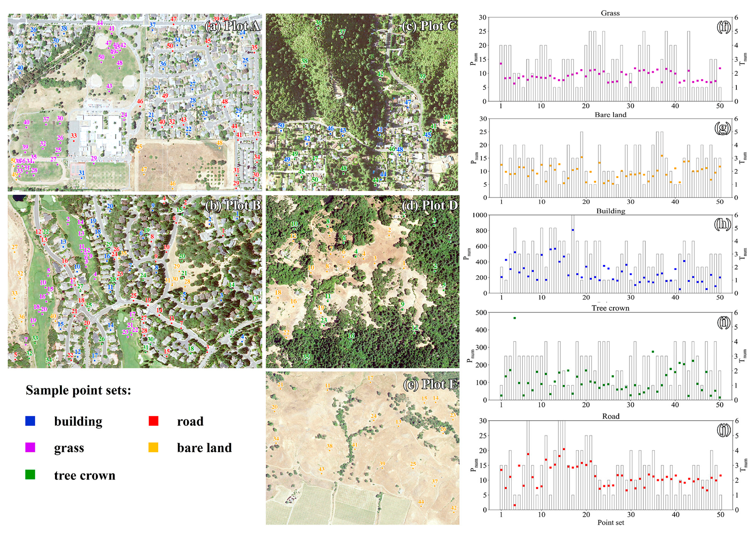
2.1. Study Sites

The study sites were located in Sonoma County, where is in northwestern California, the USA (Figure 1). We selected five plots, including three urban plots and two mountainous plots on the slope. There are multiple land cover types in each plot to validate the tested LRI correction methods. The statistical information of each plot is shown in

Table 1. Statistical information of five plots and their ALS data. FL_num means the number of flight lines when collecting point cloud data. MAX_scan means the maximum scan angle.

Plot	Site Condition	Area (km2)	Mean Slope (degree)	FLnum	MAXscan (degree)
A	urban	0.52	2	4	15
B	urban	0.45	9	2	20
C	forest and urban	0.57	18	5	13
D	forest and bare land	0.83	29	5	14
E	bare land	1.47	16	8	9

. Two urban plots (Plot A and B) are in Santa Rosa (122°44′41″ W, 38°27′23″ N), where is the county seat of Sonoma County. The other urban plot (Plot C) and a mountainous plot (Plot D) that has large-scale forests are near the Armstrong Redwoods State Natural Reserve. The dominant tree species are Coast redwood (Sequoia sempervirens), Douglas fir (Pseudotsuga menziesii), Coast live oak (Quercus agrifolia), and Blue oak (Quercus douglasii) [29]. Each urban plot mainly contains five land cover types, including road, building, grass, forest, and bare land. Plot E is close to bare land with a mean slope of about 16°.

2.2. ALS Data Collection

A compact laser-based system (ALS70-HA and ALS50-HA, Leica Geosystems AG, Heerbrugg, Switzerland) with the laser pulse wavelength of 1064 nm was used to collect discrete point cloud data on sunny days from 28 September to 28 October 2013. The scan angle was set lower than 30° during the data acquisition. All ALS data were collected at the flying altitude of 900 m. The overlapping rate between neighbor flight lines was set higher than 60%. Up to fourth-return signals were interpreted and recorded as the discrete ALS data in the LAS V1.2 format. By using 873 checkpoints to evaluate the vertical accuracy across the entire study area, the RMSE of vertical accuracy was 0.03 m (0.05 m at the 95% confidence level). Each point was automatically distinguished as a point from building, tree crown, or ground and denoted by different codes in the ALS datasets. However, the points from grass, bare land, and road were denoted as the ground type. The original pointwise LRI values were normalized into the range of [0, 255]. The pointwise 3-band true color information (in RGB format) and timestamp (the GPS time tag at which the data receiver acquired the laser return signals) were recorded as well. More detailed information about the data collection process and original ALS datasets used in this research can be found and open-source downloaded at http://sonomavegmap.org/.

2.3. The LRI Correction Method

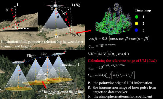
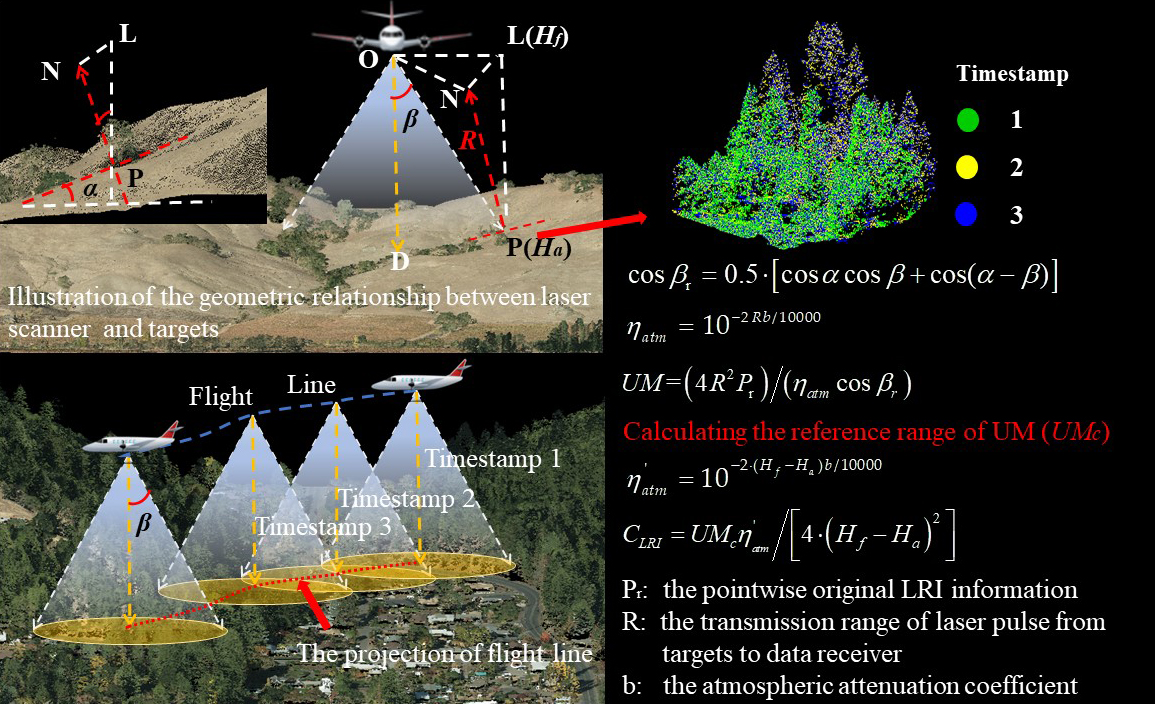
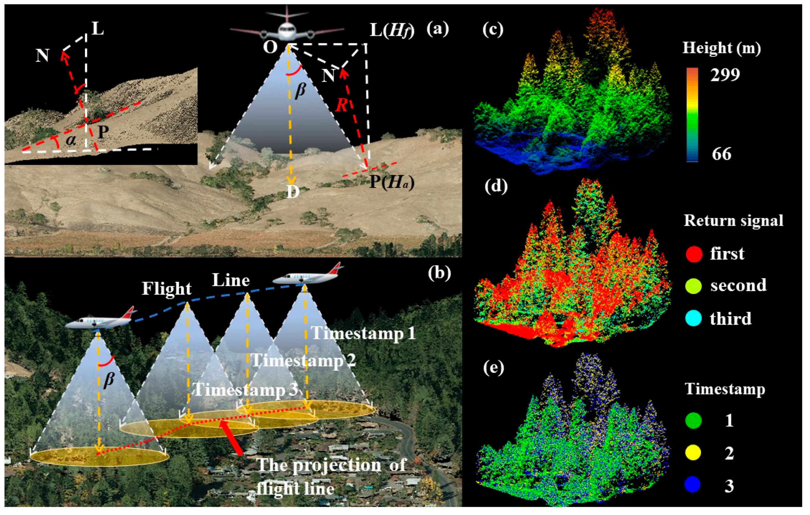
2.3.1. Background: The Simplified Radar Equation

The Radar Equation is the physical basis for interpreting the laser return signals into pointwise LRI information from a discrete ALS dataset [30]. The parameters of the simplified Radar Equation (Equation (1) include the real-time sensor-related metrics, environmental parameters, and backscatter reflectance of targets to the laser pulse [19,31]:

$$P_{\mathrm{r}}=\frac{P_t{D}_r^2{\eta }_{atm}{\eta }_{sys}\rho }{4R^2}\cos \beta ,$$

(1)

where P_t is the real-time transmitted power of laser pulse (in W), D_r is the aperture diameter of laser return signal receiver (in m), η_sys is the sensor-specific transmission factor (dimensionless), ρ is the backscatter reflectance of target to the laser pulse (dimensionless), R is the transmission range of laser pulse from targets to return signal receiver (in m), β is the scan angle (the angle at which the laser pulse emitting from the laser scanner, degrees), and η_atm is the atmospheric transmission factor (dimensionless). Theoretically, the pointwise LRI value from one ground object with a near-Lambertian surface is related to its R and ρ if the sensor-related metrics were invariable during the ALS data collection. However, η_atm and P_t are changeable when using a laser scanner having an embedded adjustment tool for sensor-related parameters, such as the AGC tool, while these two parameters are not pointwise recorded in a discrete ALS data. The altitude of each point (H_a) and its β value are recorded in the LAS file. We calculated η_atm by Equation (2):

$${\eta }_{atm}={10}^{-2Rb/10000},$$

(2)

where b = the atmospheric attenuation coefficient (in dB/km). Here, the b was set as 0.22 [14].

2.3.2. LRI Correction Methods

We designed a local median filter (LMF) method to point-by-point correct the LRI information from discrete ALS data. Presuming that the first-return points of trees are all from the canopy surface [23,31], we extracted those data relying on their classification and return-type codes stored in the LAS file (V1.2 version). As the return signal reflector within a forest canopy is always a mixture of woody and foliage components, we maintained the pointwise original LRI information of other returns from the inner canopy in the correction results. For ground objects except for tree crowns, we corrected their all-return LRI information by the following methods:

A. Calculating the Local Slope of Targets

We used the sphere searching method with a searching radius of 1.5 m to extract the local point set K = {p_i(x_i, y_i, z_i), i = 1, 2,…, n} for each point. Then, we pointwise calculated the local slope for each point, except for those points from tree crowns. In a local point set, the mean coordinatefor $\stackrel{\rightharpoonup }{C}$ for the n points in K was calculated as:

$$\stackrel{\rightharpoonup }{C}=\left(1/n\right)\cdot {\displaystyle \sum _{i=1}^n{\left(x_i,y_i,z_i\right)}^T},$$

(3)

and the local slope of target covered by n points in K could be calculated as:

$$Slope=(1/n)\cdot {\displaystyle \sum _{i=1}^n\arctan \left[\left|z_i-z_c\right|/\sqrt{{(x_i-x_c)}^2+{(y_i-y_c)}^2}\right]}.$$

(4)

Here, (x_c, y_c, z_c) is the Cartesian coordinate of the center point within a searching unit. When calculating the local slope of rooftops, we based on the pointwise classification codes stored in the LAS V1.2 file to remove the nearby points of ground in each searching unit. The height difference between rooftops and the ground surface might cause an overlarge slope near the boundaries of buildings. Similarly, we removed the points of buildings when calculating the local slope of road, bare land, and grass.

B. Calculating the Laser Incidence Angle

The surface slope of targets and scan angle (β) affect the incidence angle of laser return signal. As shown in Figure 2, the flight altitude of the laser scanner is H_f m (H_f = 900 for tested ALS dataset), NP is the normal vector of point P on the surface with the altitude of H_a m. The local slope (∠NPL) is equal to α°. For points with β equal to 0°, their locations are on the projection of flight lines of the laser scanner during the data collection (shown as the red dashed line in Figure 2b). However, for some clipped datasets that do not contain the projection of flight lines, we could not calculate the range between the emitting point of the laser pulse (O) and its sub-stellar point D and the angle ∠OLN. Owing to the fact that the distance OP can be calculated by β and LP, we deduced the variation range of ∠OPN, that is the incidence angle of laser return signal (β_r) [31]:

In ΔNPL and ΔOPL:

$$NP=\left(H_f-H_a\right)/\cos \alpha ,$$

(5)

$$OP=\left(H_f-H_a\right)/\cos \beta ,$$

(6)

$$NL=\left(H_f-H_a\right)\tan \alpha ,$$

(7)

$$\mathrm{and} OL=\left(H_f-H_a\right)\tan \beta .$$

(8)

Based on the law of cosines,

$$O{P}^2+N{P}^2-2(OP)(NP)(\cos \angle OPN)=N{L}^2+O{L}^2-2(NL)(OL)(\cos \angle OLN).$$

(9)

Substituting (5) to (8) into (9):

$$\cos {\beta }_r=\left(1+\tan \alpha \tan \beta \cos \angle OLN\right)\cos \alpha \cos \beta ,$$

(10)

the incidence angle could be calculated as:

$${\beta }_r={\cos }^{-1}(\cos \alpha \cos \beta +\sin \alpha \sin \beta \cos \angle OLN).$$

(11)

When using historical ALS data, users may only clip a part of the point cloud from the whole database, such as the point cloud data we used in this study. For each point, the clipped point cloud may not contain the projection of receiving the point of laser return signal (collected at the same timestamp and with 0° incidence angle, such as point D in Figure 2), especially for points at the edge of the clipped range. Another case is that multiple points were chosen as the projection of the receiving point as they collected at the same timestamp and with 0° incidence angle. Once the projection point cannot be extracted, or more than one point is selected, the azimuth of the laser return signal cannot be calculated. As shown in Figure 2, if $\angle OLN$ > 90°, the sensor cannot receive return signals from targets. Thus,

$$\cos {\beta }_r\in \left[\cos \alpha \cos \beta ,\cos (\alpha -\beta )\right],$$

(12)

and we calculated $\cos {\beta }_r$ as:

$$\cos {\beta }_{\mathrm{r}}=0.5\cdot \left[\cos \alpha \cos \beta +\cos (\alpha -\beta )\right].$$

(13)

C. The LRI Correction for Non-Forest Points

For non-forest points, we used β_r to replace β [21] in Equation (1). The product of unrecorded sensor-related measurements in ALS datasets (UM) is calculated as:

$$UM=P_t{D}_{\mathrm{r}}{}^2{\eta }_{sys}\rho =\left(4R^2{P}_r\right)/\left({\eta }_{atm}\cos {\beta }_r\right),$$

(14)

where P_r means the pointwise original LRI. Assuming that $\rho$ of local points in one searching unit were similar, we built the KD-tree index for the original ALS data to search the nearest four points for each point. Then, we calculated the reference range of UM for each point as [UM_min, UM_max]:

$$U{M}_{\min }=U{M}_{q1}-1.5\cdot U{M}_{QR},$$

(15)

$$U{M}_{\max }=U{M}_{q3}+1.5\cdot U{M}_{QR},$$

(16)

where UM_q1 and UM_q3 are the lower (i.e., 25%) quartile and upper (i.e., 75%) quartile of the nearest four UM values, respectively. The UM_QR means the interquartile range of four UM values [32]. We kept the original UM for the kernel point if it was within the reference range to avoid excessive correction. Otherwise, we used the local median UM value to replace it. The pointwise scan angle was extracted by the Laspy 1.5.1 software package (https://github.com/grantbrown/laspy) in Python 3.5 program environment.

Here, we redefined R as the vertical range between H_f and H_a to avoid setting a subjective reference plane for LRI correction. Finally, we recalculated LRI (LRI_C) point-by-point as:

$$LR{I}_C=U{M}_C{\eta }_{{}_{atm}}^{\prime }/\left[4\cdot {\left(H_f-H_a\right)}^2\right],$$

(17)

$${\eta }_{atm}^{\prime }={10}^{-2\cdot (H_f-H_a)b/10000},$$

(18)

where UM_C means the post-corrected UM. Thus, the correction results simulated the pointwise LRI information interpreted from the laser return signal with a 0° incidence angle and post-corrected UM. However, the original LRI would be kept for points with LRI_C over the predefined range of LRI values (from 0 to 255 for the tested ALS data).

D. The LRI Correction for Points from Tree Crowns

The incidence angle of laser return signals from tree crowns could not be deduced. For each first-return point from tree crowns, we used the method described in the previous section to search its nearest four first-return points. Then, we judged whether the LRI value of the center point in one searching unit was in its reference range. If its LRI value was within the range of $\left[LR{I}_{q1}-1.5\cdot I_{QR},LR{I}_{q3}+1.5\cdot I_{QR}\right]$ (LRI_q1 and LRI_q3 mean the lower and upper quartile of local four LRI values, and I_QR means the interquartile range of four LRI values), we maintained its original LRI. Otherwise, we used the local median LRI to replace its original LRI value. We programmed the LMF and RN correction methods in Python 3.5 using the Scikit-Learn 0.21.3 package [33].

2.4. The LRI Correction Results Evaluation

2.4.1. Random Sampling and Evaluation

To evaluate the LRI correction methods, we selected point sets from five land cover types. The points in each sample point set (with an area of 3 m $\times$ 3 m) were from the same land cover type. For points from one point set (from road, bare land, grass, tree crown, or building), the similarity among their post-corrected LRI values should be higher. Then, we calculated the mean ($\mu$), standard deviation ($\sigma$), and coefficient of variation (CV) of pointwise LRI for each point set:

$$CV=\sigma /\mu .$$

(19)

Furthermore, we used the coefficient of joint variation (CJV) [21] to evaluate the discrepancy of LRI information between two types of point sets (W and V). As some CJV values might overlarge if the average LRI values of pairs of point sets are close to each other, we optimized its calculating method as:

$$CJV=e^{\left|\mu (W)-\mu (V)\right|/{\left(\sigma (W)+\sigma (V)\right)}^2}-1.$$

(20)

Here, a higher CJV shows less between-class confusion of pointwise LRI information from W and V point sets.

The emission time tag of each laser pulse was not stored during the ALS data collection. Considering the propagation speed of the laser pulse (about 3 × 10⁸ m/s), we ignored the time difference between the emitting and receiving time of a laser pulse. Thus, we assumed that the points collected at the same timestamp were with the same UM. For each point set, we calculated the mean CV (T_CV) and mean CJV (T_CJV) of LRI values collected at different timestamps, except for those collected at only one timestamp.

$$T_{CV}=\left(1/N\right)\cdot {\displaystyle \sum _{i=1}^N\sigma (B_i)/\mu (B_i)}(N>1),$$

(21)

$$T_{CJV}=\left[2/(N-1)\cdot N\right]\cdot {\displaystyle \sum _{w,m\in N}^{(N-1)\cdot N/2}(e^{\left|\mu (B_w)-\mu (B_m)\right|/{\left(\sigma (B_w)+\sigma (B_m)\right)}^2}}-1)(N>1,w>m),$$

(22)

where N means the number of timestamps when collecting each point set, and B means the pointwise LRI values collected at the same timestamp. With the decreasing T_CV and T_CJV, the similarity among LRI values obtained at N timestamps would increase.

2.4.2. Land Cover Classification

To evaluate the contribution of LRI correction methods, we manually chose points from road, bare land, and grass as the training and test samples, which were all distinguished as ground type in the original datasets. There was no intersection between training and test points. We used the Laspy 1.5.1 software package to extract the points of ground type by the pointwise classification code stored in the LAS file. For training points, we combined their original, LMF-corrected, or RN-corrected LRI with the pointwise 3-D true color information to form the 4-D feature matrices as the input to the random forest (RF) classification model [34]. The RF classifier was programmed using the Scikit-Learn 0.21.3 [33]. We removed points from tree crowns and buildings, as they had been distinguished in the original datasets. Finally, we calculated the overall classification accuracy (OA), producer’s accuracy (PA), and user’s accuracy (UA) of points from each land cover type and the Kappa coefficient (κ) for the classification results. McNemar’s test [35] was used to evaluate the statistical significance between the classification results obtained by using different types of LRI information (original, LMF-corrected, or RN-corrected).

$$OA=\left(V_{RO}+V_L+V_G\right)/\left(T_{RO}+T_L+T_G\right),$$

(23)

$$PA=V_{type}/T_{type},$$

(24)

$$UA=V_{type}/\left(V_{type}+F_{type}\right),$$

(25)

where V_type means the number of test points that were correctly classified (RO: road, L: bare land, G: grass) in ALS data of one plot. T_type is the number of tested points from type V in the same dataset. F_type is the number of test points misclassified as type V in the same dataset. The κ statistic is computed as:

$$\kappa =\left(P_0-P_c\right)/\left(1-P_c\right),$$

(26)

$$P_0={\displaystyle \sum _{i=1}^r{X}_{ii}}/N,$$

(27)

$$P_c={\displaystyle \sum _{i=1}^r\left(X_{i+}\cdot X_{+i}\right)}/N^2,$$

(28)

where P₀ means the relative observed agreement among N samples in error matrices with r rows. P_c is the hypothetical probability of chance agreement. X_i+ and X_+i are the row probabilities and the column probabilities, respectively.

3. Results

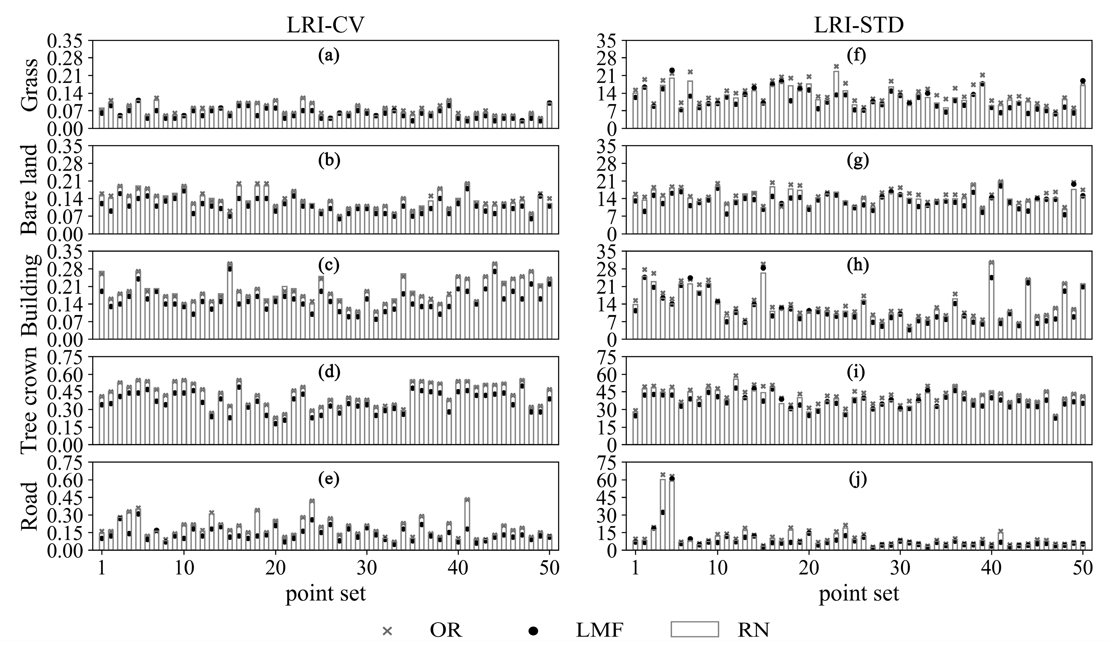
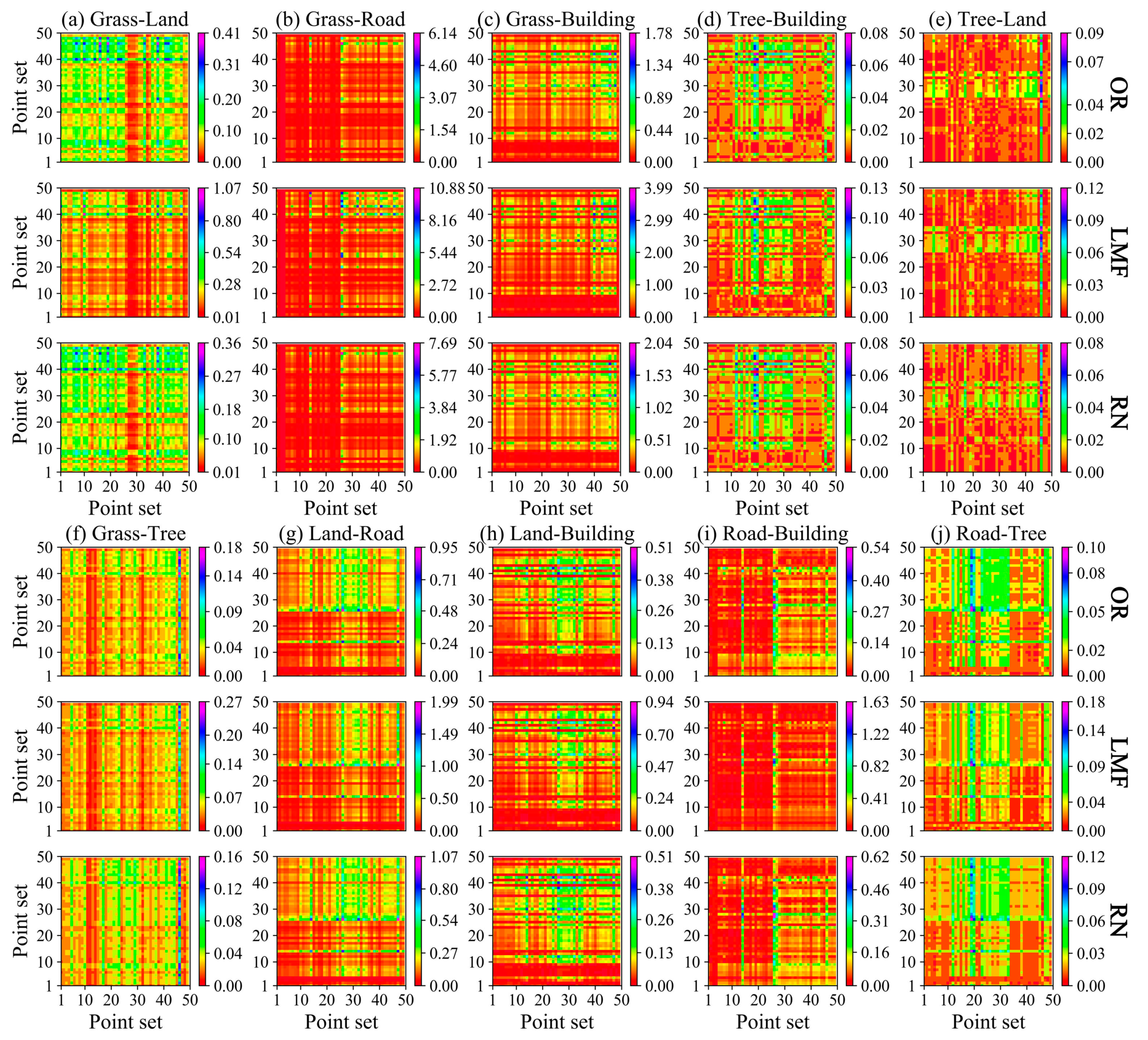
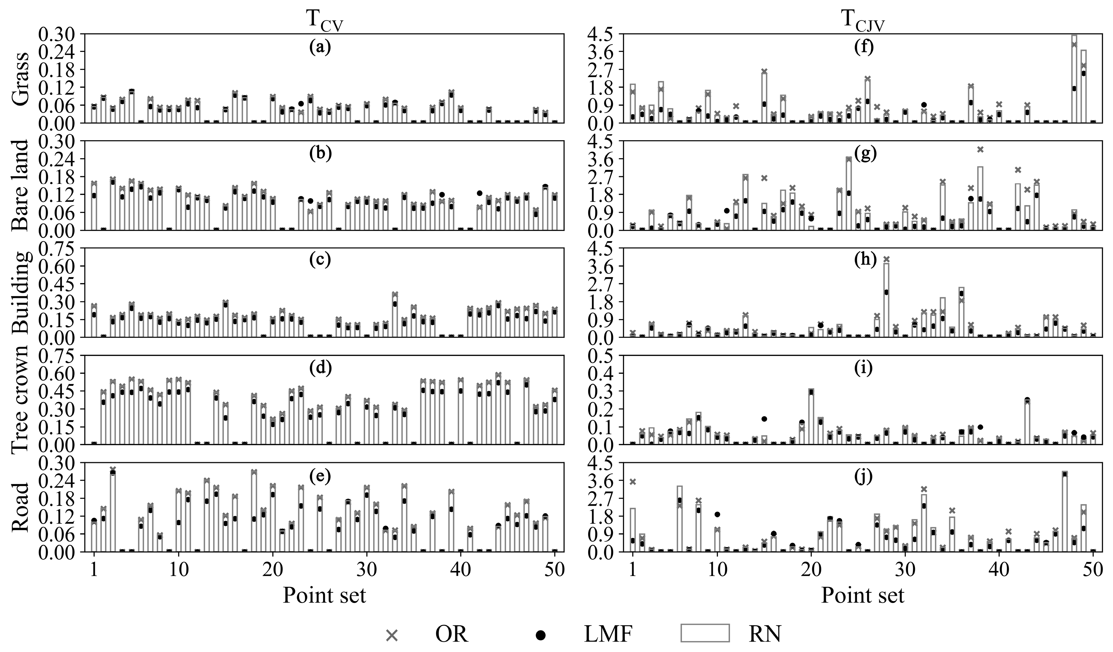
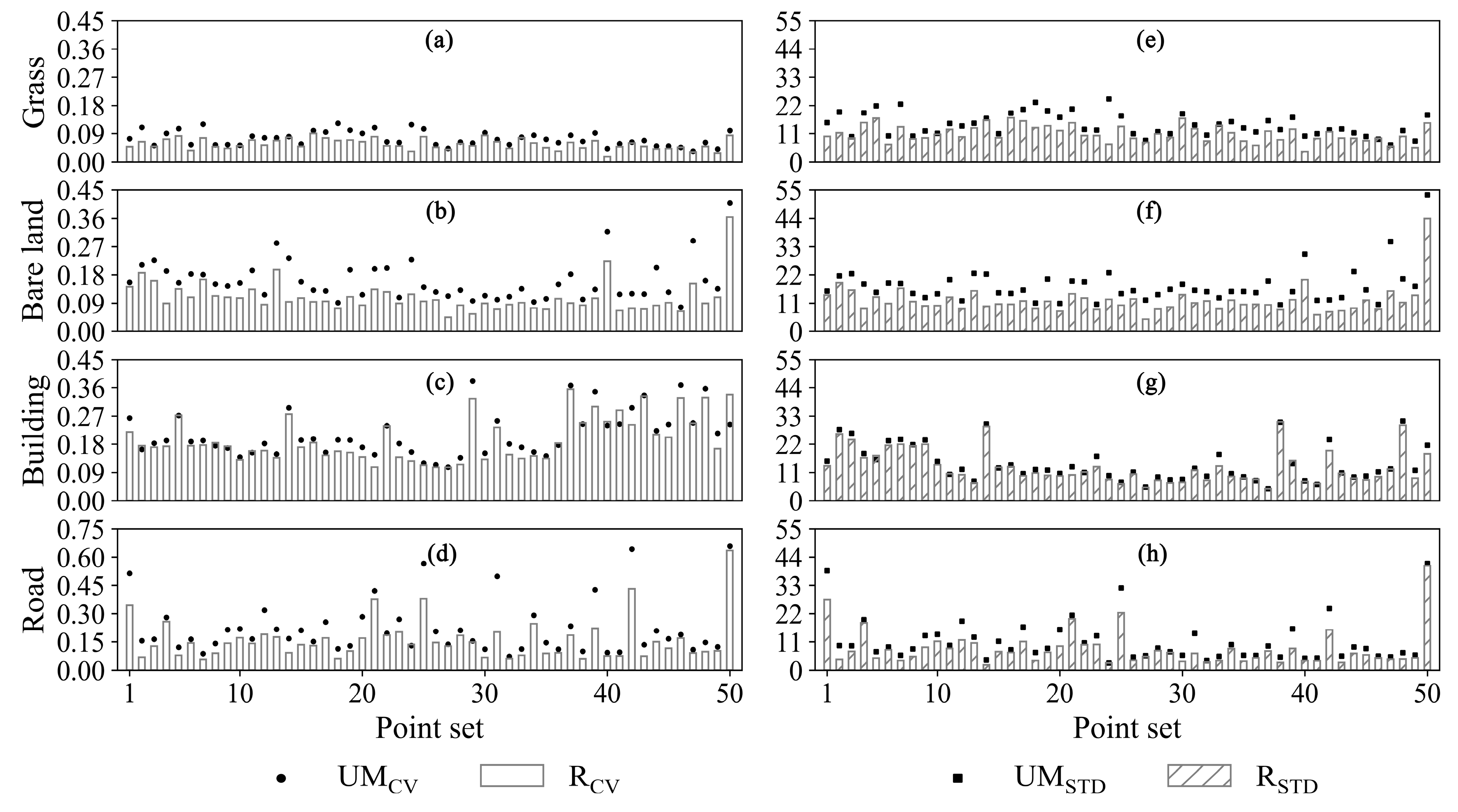
3.1. The LRI Correction Results of Sample Point Sets

The location of each point set is shown in Figure 3 as well as the number of timestamps and point density (the average number of points per square meter) information. The standard deviation (LRI-STD) and CV (LRI-CV) of original, LMF-corrected, and RN-corrected LRI information from each point set (total 250 point sets) selected in Plots A, B and C are shown in Figure 4 and

Table 2. Statistical information about the STD and CV of pointwise LRI values from selected point sets. Here, OR, LMF, and RN mean the original LRI information, the LRI information corrected by the local median filter method, and the LRI information corrected by the range-normalized method, respectively.

Types	LRI	LRI-STD		LRI-CV
		Max	Mean	Max	Mean
Grass	OR	24.60	14.33	0.12	0.07
	LMF	23.06	11.32	0.11	0.06
	RN	22.55	12.41	0.12	0.07
Bare land	OR	20.73	15.27	0.20	0.14
	LMF	19.76	13.03	0.18	0.11
	RN	20.73	14.44	0.20	0.13
Road	OR	66.46	11.43	0.43	0.19
	LMF	60.91	8.21	0.31	0.14
	RN	60.25	10.13	0.44	0.19
Building	OR	30.55	14.17	0.30	0.19
	LMF	28.35	12.03	0.28	0.15
	RN	30.60	13.11	0.30	0.19
Tree crown	OR	58.85	41.85	0.55	0.43
	LMF	48.18	36.55	0.50	0.36
	RN	55.84	39.66	0.56	0.43

. Each land cover type contains 50 sample point sets.

As shown in Figure 4, over 94% of point sets have lower LRI-CV and LRI-STD after the LMF correction than those of the original LRI information. Although over 72% of the RN-corrected point sets from five land cover types had lower LRI-CV, the LRI-STD of more than 70% of point sets witnessed increasing, which means the similarity of pointwise LRI values became lower after the RN correction. For a point set, using the LMF correction method could more robustly increase the similarity of LRI values (with decreasing LRI-CV and LRI-STD) compared to using the RN method.

The average LRI-STD dropped relatively severely for point sets from tree crowns but slightly for those from buildings and bare land in the LMF-corrected results. In Table 2, the mean LRI-STD decrease by 3.01 for point sets from grass, by 2.24 for point sets from bare land, by 3.22 for point sets from road, by 2.14 for point sets from buildings, and by 5.3 for point sets from tree crowns after being corrected by the LMF method. The LRI-CV of each point set also decrease after using the LMF correction method. The mean LRI-CV values decrease by 0.01 for point sets from grass, by 0.03 for point sets from bare land, by 0.04 for point sets from buildings, by 0.05 for point sets from road, and by 0.07 for point sets from tree crowns. However, the LRI-CV of each point set was nearly invariable after the RN correction compared with those of the original LRI information.

The confusion of LRI information between each pair of point sets from diverse land types was decreased after the LMF correction. As shown in

Table 3. Statistical analysis concerning the LRI-CJV for each pair of point sets from diverse land cover types (ten combinations).

Types	LRI	LRI-CJV		Types	LRI	LRI-CJV
		Max	Mean			Max	Mean
Building vs. Grass	OR	1.78	0.22	Grass vs. Bare land	OR	0.41	0.11
	LMF	3.99	0.41		LMF	1.07	0.16
	RN	2.04	0.25		RN	0.36	0.10
Building vs. Road	OR	0.54	0.06	Grass vs. Tree crown	OR	0.18	0.03
	LMF	1.63	0.15		LMF	0.27	0.05
	RN	0.62	0.07		RN	0.16	0.03
Building vs. Bare land	OR	0.51	0.08	Road vs. Bare land	OR	0.95	0.14
	LMF	0.94	0.18		LMF	1.99	0.24
	RN	0.51	0.08		RN	1.07	0.17
Building vs. Tree crown	OR	0.08	0.01	Road vs. Tree crown	OR	0.10	0.02
	LMF	0.13	0.02		LMF	0.18	0.03
	RN	0.08	0.01		RN	0.12	0.02
Grass vs. Road	OR	6.14	0.41	Bare land vs. Tree crown	OR	0.09	0.01
	LMF	10.88	0.93		LMF	0.12	0.01
	RN	7.69	0.51		RN	0.08	0.01

, for each pair of point sets selected from two land cover types except tree crowns, the mean LRI-CJV increase over 0.05 after the LMF correction compared to those from the original LRI information. However, the average LRI-CJV rising slightly (< 0.03) for pairs of point sets, including one from the tree crown. In the RN-corrected results, the mean LRI-CJV values increase slightly or keep invariable except for the pairs of point sets from grass and bare land. In Figure 5, we illustrated the result that the LRI-CJV values were always higher in the LMF-corrected results than those of the RN-corrected LRI information. Thus, the discrepancy in LRI information between each pair of point sets from diverse land cover types was relatively more significant in the LMF correction results, compared with those in the original and the RN-corrected LRI information.

As shown in Figure 6 and

Table 4. T_CV and T_CJV of LRI information from point sets collected within multiple timestamps. The data in the last four columns show the number of point sets that meet the condition shown in parentheses. For example, the T_CV (LMF ≤ OR) means the number of point sets in which the T_CV of LMF-corrected LRI information is lower than or equal to those of the original LRI information (OR).

Types	Number	LRI	Mean TCV	Mean TCJV	TCV (LMF≤OR)	TCV (LMF≤RN)	TCJV (LMF≥OR)	TCJV (LMF≥RN)
Grass	34	OR	0.06	0.98	29	30	32	31
		LMF	0.06	0.50
		RN	0.06	0.99
Bare land	41	OR	0.11	1.19	36	36	38	38
		LMF	0.10	0.62
		RN	0.11	1.06
Road	37	OR	0.15	1.08	31	32	29	30
		LMF	0.12	0.83
		RN	0.15	1.08
Building	40	OR	0.19	0.57	40	40	35	37
		LMF	0.16	0.38
		RN	0.19	0.58
Tree crown	38	OR	0.43	0.08	38	38	30	30
		LMF	0.36	0.07
		RN	0.43	0.08

, over 82% of the point sets have lower T_CV values after the LMF correction compared to those of the original and RN-corrected LRI. In the LMF-corrected results, the mean T_CV decrease by nearly 0.03 for point sets from road and building, by 0.07 for point sets from tree crowns, and by 0.01 for point sets from bare land. However, the mean T_CV of each point set from grass is nearly invariable after the LMF correction. In addition, the most significant declines of T_CV are 0.16 for point sets from road, 0.12 for point sets from tree crown, 0.08 for point sets from buildings, 0.04 for point sets from bare land, and 0.025 for point sets from grass after the LMF correction than using the original LRI information (shown in Figure 6a–e). It should be noted that the T_CV of each point set was almost unchanged after the RN correction. We found that the average T_CJV only decreased for point sets from bare land in the RN-correction results, but all types of point sets in the LMF-corrected results. As shown in Figure 6, the T_CJVs become lower for over 78% of the tested point sets when using the LMF method compared to those of the original and RN-corrected LRI. The average T_CJVs of LMF-corrected results drop dramatically for point sets from bare land (by from 1.19 to 0.62). Still, they vary slightly for those from tree crowns due to the high similarity (the average T_CJV = 0.07) of the original LRI information collected at different timestamps. For over 78% of the point sets collected within multiple timestamps, the similarity of pointwise LRI values was higher after the LMF correction than those corrected by the RN method.

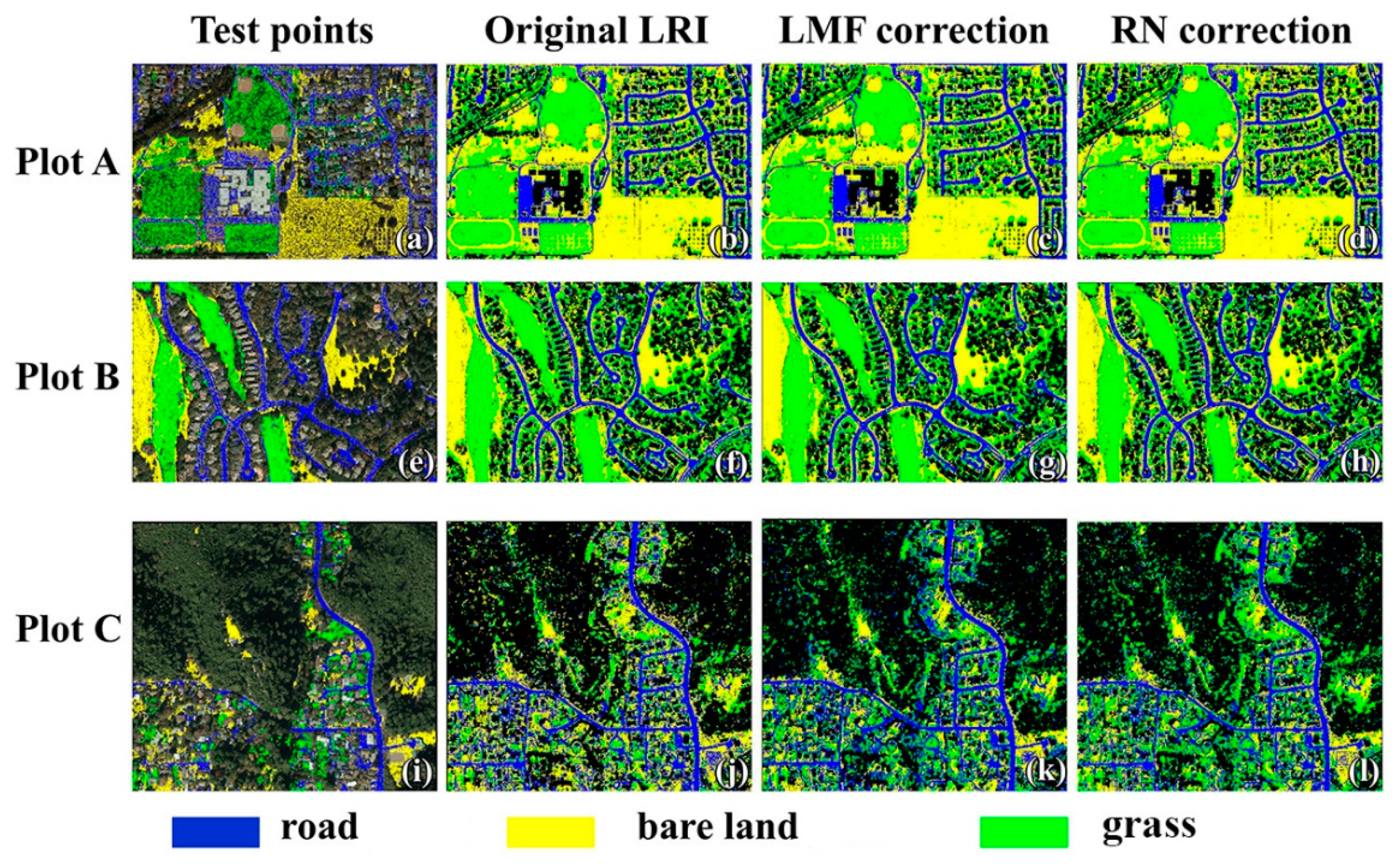
3.2. The Classification Accuracy of Ground Points

In Plots A, B, and C, we manually selected 30,000 test points for each of the three land cover types, including bare land, road, and grass, that were all denoted as ground type in the original LAS file. Then, the 90,000 test points were used to assess the classification accuracy of ground points by using the original and post-corrected (LMF- and RN-corrected) LRI information and the pointwise true color information. All results are shown in Figure 7 and

Table 5. Classification accuracy of grass, bare land, and road points. The OA means the overall classification accuracy. The G-PA, L-PA, and RO-PA mean the producer’s accuracy of tested points from grass, bare land, and road, respectively. The G-UA, L-UA, and RO-UA mean the user’s accuracy of tested points from grass, bare land, and road, respectively. By the McNemar’s test, the difference between each pair of classification results was significant with p < 0.05.

Plot	LRI	OA (%)	G-PA (%)	L-PA (%)	RO-PA (%)	G-UA (%)	L-UA (%)	RO-UA (%)	$\mathit{\kappa }$
A	OR	79.59	79.56	63.58	95.63	94.33	92.10	65.21	0.69
	LMF	81.83	83.01	64.36	98.12	97.46	95.56	66.52	0.73
	RN	80.32	80.80	64.80	95.35	94.22	93.32	65.84	0.70
B	OR	86.11	94.12	72.08	92.13	91.53	95.11	75.88	0.79
	LMF	88.65	97.41	74.04	94.49	94.51	98.24	77.72	0.83
	RN	87.29	94.84	74.36	92.67	92.86	95.17	77.40	0.81
C	OR	82.35	76.14	93.68	77.22	93.35	81.44	74.66	0.74
	LMF	85.27	76.71	95.55	83.56	95.91	85.96	76.75	0.78
	RN	82.90	77.20	90.45	81.04	93.08	83.92	74.15	0.74

. Using the corrected LRI could effectively increase the OA by about 3% (κ ≥ 0.73, p < 0.05) compared with the OA of using the original LRI information. Using the LMF-corrected LRI was better than the RN-corrected LRI for classifying ground points. The PA of road points (RO-PA) were higher in the classification results of Plots A and B by using the LMF-corrected LRI, while this index was lower than 84% when using different types of LRI information to distinguish the data of Plot C. The PA values of grass points (G-PA) were nearly invariant for the classification results of Plot C when using three types of LRI information. Still, this index increased by over 3% for the classification results of Plots A and B after using the LMF-corrected LRI information. The G-PA was slightly higher when using the RN-corrected LRI information to classify the ALS datasets of Plots C than using the LMF-corrected LRI information. The PA of points from bare land (L-PA) increased by less than 2% when using the post-corrected LRI. For the classification results of Plot C, the L-PA of LMF-corrected data increased by nearly 2% compared to those using the original LRI and by over 5% compared to those using the RN-corrected LRI. Thus, using the LMF-corrected LRI achieved higher accuracy when classifying the above three land cover types.

4. Discussion

4.1. Sensitivity Analysis: R vs. UM

According to Equation (1), increasing the transmission range (R) of the laser return signal would reduce the LRI value. The scanning angle, surface slope, and altitude of ground objects affect the variables θ_r and R of the laser return signal [20,36,37]. For point cloud data from a near-Lambertian surface, the variable scanning angle might be the main reason for a reduction in the similarity of pointwise LRI information from the same land cover type. However, the effects of variable UM to the pointwise LRI information are rarely explored in most range-based correction methods.

We calculated the mean STD and CV of the original pointwise LRI information collected at the same timestamp but with different R values (R_STD and R_CV) or with similar R values but changeable UM (UM_STD and UM_CV) in each point set from four land cover types. The points with a difference in R-values less than 0.1 m were assumed as points collected with similar R. We used the average values of these four metrics to do the sensitivity analysis, as each point set might contain multiple UM_STD, UM_CV, R_STD, and R_CV values. The results are shown in Figure 8 and

Table 6. Largest UM_STD, UM_CV, R_STD, and R_CV of LRI information from point sets except for those from tree crowns. The UM_STD and UM_CV mean the average LRI-STD and LRI-CV for points collected with the similar transmission range of laser return signal (R) at different timestamps in each point set. The R_STD and R_CV mean the average LRI-STD and LRI-CV for pointwise LRI information collected at the same timestamp but different R in each point set.

Types	Max UMSTD	Max UMCV	Max RSTD	Max RCV
grass	24.60	0.12	17.16	0.09
road	41.54	0.66	40.19	0.60
building	31.04	0.36	29.13	0.29
bare land	53.04	0.41	43.89	0.36

, in which the R_STDs and R_CVs of point sets collected at only one timestamp were calculated. In addition, we removed the point sets from tree crowns where the local points rarely had similar R during the sensitivity analysis.

We found that the UM introduced more noise than R to the original LRI information from the ALS datasets of Plots A to E. The UM_STD was larger than R_STD for each point set from four land cover types except for about 30% of the point sets from buildings. In addition, the UM_CV was slightly larger than R_CV for each point set except for 26% of the point sets from buildings. The UM_CV of LRI information from point sets of grass were lower than from the other three land cover types (i.e., bare land, building, and road). When using the laser pulse in the 1064-nm wavelength, the backscatter reflectance (ρ) of grass is theoretically higher than those of targets without vegetation coverage [38,39]. The AGC tool would adjust the sensor-related metrics when the data receiver could not capture laser return signals from targets with low ρ. It is reasonable that the average variable rate of pointwise LRI values with similar R collected at multiple timestamps from grass was lower than those from the other three land cover types (with lower UM_CV). We inferred that the variable UM might introduce more noise to the pointwise LRI information from targets with low ρ.

4.2. Comparison with the RN Method

The RN method is commonly used to correct the LRI information of discrete ALS data [3,40]. However, we found that the RN method contributed less than the LMF method in correcting the LRI information of tested ALS data. The RN and LMF methods both calculate R to correct the energy attenuation of laser return signals. When using the RN method, we set R as the difference in height between H_f and H_a. Thus, the index R used for the RN and LMF correction is equal. With the assumption that the variable R causes the outliers of LRI, the RN-corrected LRI values collected with similar R from the same targets should be the same. However, this was not the case for selected point sets.

Whether to assume that the pointwise UM values are invariable during the LRI correction is the main difference between the RN and LMF methods. Using the LMF correction method can detect the outliers of pointwise variable UM in original ALS data and replace them to suppress the noise caused by the variable sensor-related metrics. The original pointwise UM would be maintained if it was within its local reference range to avoid an excessive LRI correction. As shown in Figure 4, the LRI-STD and LRI-CV of RN-corrected results were always higher than those corrected by the LMF correction method. For ALS data collected with the fixed UM, using the RN and LMF methods can achieve the same results.

We also calculated the T_CV and T_CJV for point sets collected at multiple timestamps. Since the points in the same point set are of the same type and are distributed in the range of 3 m×3 m, their pointwise LRI values should be similar. For the point sets that were collected at more than one timestamp, the variable UM reduced the similarity of pointwise LRI values. As shown in Table 4 and Figure 6, the T_CV and T_CJV values were always higher for the original LRI information. It is sensible that the similarity of LMF-corrected LRI collected at different timestamps was increased (with lower T_CV and T_CJV) for over 78% of the tested point sets, compared with those of the original and RN-corrected LRI information. When using a laser scanner that can automatically adjust the emitting power of laser pulse (e.g., the ALS50-HA), it is necessary to suppress the noise introduced by the variable transmission range of return signals and sensor-related parameters. The results of this study also verify that using the LMF method can robustly correct the LRI information interpreted by different laser scanners.

4.3. The Sources of Outliers in the LMF-Corrected LRI Information

After the LMF correction, the LRI values of some points might surpass their predefined range from 0 to 255. Through visual detection, these points were always at the edges of rooftops, or grass area, or on the surfaces of vehicles parked on the road, but they were seldom from road and bare land. Yan and Shaker [21] also found some overlarge LRI values from grass and rooftops after the LRI correction. Furthermore, the LRI values of some points from tree crowns, which were misclassified as ground type in original ALS datasets, might be overlarge after the LMF correction.

We inferred that the sources of outliers were as follows: (1) we hypothesized that the flying altitude of the laser scanner was invariant during the data collection. However, the real-time flying altitude was not recorded in discrete ALS datasets. For return signals collected with lower R, the corresponding interpreted LRI values would be higher according to Equation (1) [41]. (2) The pointwise LRI values from targets with high ρ are larger than those from targets with lower ρ in theory. For example, the LRI values of points from tree crowns are higher than those of points from asphalt road when using the near-infrared laser pulse. Thus, we might not precisely detect the reference range of UM for some points on the boundaries of targets. (3) Setting the exponent of the denominator in Equation (1) as two (squared) is only suitable for the reflectors with near-Lambertian surfaces [3]. However, existing research has verified that this setting is not ideal for correcting LRI values from targets with a linear or point distribution, such as suspended electrical wires or upright stumps [19]. (4) The LRI information of scan targets located in the overlapping region of LiDAR data strips may be affected by line-stripping noise [21]. (5) The hotspot effect of received laser return signals. The LRI values dramatically increase naturally toward the zero-phase angle between the laser scanner and viewing directions. Without the synergy field survey for the ρ of ground objects to the laser pulse, we cannot quantitatively assess the hotspot effects of LRI information for historical ALS data. Moreover, the hotspot effect on LRI information seems more severe for near-infrared laser pulses according to the laboratory tests [17]. Thus, for points with overlarge post-corrected LRI values (>255), we maintained their original LRI in the results.

4.4. Limitations and Potential Applications

The LMF method is not suitable for correcting the LRI information interpreted from more than first-return signal from tree crowns, in which the return signals might be reflected from understory shrubs and soil background with diverse ρ. Thus, we did not calculate the UM for points from tree crowns, but replaced the outliers of related LRI information by their local median value. However, it should be noted that the relationship between the pointwise post-corrected LRI value and corresponding ρ was still unknown for historical ALS data [42].

When calculating the reference range of UM for non-forest points or LRI value for first-return points from tree crowns, we assumed that points in one searching unit have similar ρ. However, the reflectance among adjacent points may be different if the local point density was low, as they may from multi-class objects. We inferred that the variable local point density had an impact on the LRI correction results. To evaluate the effect of point density on the LRI correction results, we must consider the geometrical features of objects and the complexity of land cover types. It is challenging to evaluate the lowest available point density for ALS data collected by different laser scanners and from diverse regions. Assessing the effects of point density on the LMF correction results should be carried out by synchronously surveying the backscatter reflectance of ground objects to the emitting laser pulse during the data collection. At present, we cannot carry out this study by using a historical ALS dataset without a field survey of the backscatter reflectance of ground objects. We will attempt to do this in our future research.

The LRI-STD and LRI-CV of point sets from the same land cover type experienced a reduction after using the LMF correction method, especially for the pointwise LRI information from tree crowns, grass, and road. Using the LMF correction method could achieve higher accuracy when classifying land cover types from the ALS data. Existing research studies have attempted to use the multi-temporal and multispectral LRI information from ALS data collected in forests to reveal the spatiotemporal variation of canopy physiological and functional traits at the single crown level [43,44], for example, the chlorophyll content, the photosynthetic rate, and the equivalent water thickness of leaves [39,45]. Some studies have verified that using the corrected multispectral LRI information is superior to the multispectral images in depicting the 3-D distribution of physiological features at the singletree level in large-scale forests [12,46]. Theoretically, the LMF method also has the potential to correct the LRI information from multispectral ALS datasets, which needs to be verified in future ecological research.

5. Conclusions

To correct the pointwise LRI information from the discrete ALS dataset, we designed the LMF method, a semi-theoretical correction method without the requirement of synergy field surveys for the backscatter reflectance of targets to emitting laser pulses. Based on the simplified Radar Equation, we calculated, point-by-point, the local reference range of UM for each non-forest point, and then replaced the outliers with the local median UM to recalculate their LRI values. For the pointwise LRI from tree crowns that were beyond their reference range, we replaced these with the local median LRI values. The average LRI-CV and LRI-STD decreased by more than 0.01 and 2.14, respectively, for five types of point sets after using the LMF method. The discrepancy among the pointwise LMF-corrected LRI values from diverse land cover types became more significant (with higher LRI-CJV) compared to those corrected by the RN method and in original LRI information. Besides, for over 78% of the sample point sets, the similarity of pointwise LMF-corrected LRI values collected at different timestamps was increased (with lower T_CV and T_CJV). To classify the ground points into three land cover types (grass, road, and bare land) from ALS data, combining the pointwise LMF-corrected LRI with the 3-D true color information could increase the OA about 3% (κ ≥ 0.73, p < 0.05), compared with the results of using the original and RN-corrected LRI information. The variable pointwise UM introduced more noise than R to the original LRI information from the tested ALS data. The LMF method shows its ability to correct the outliers of LRI for the tested historical discrete ALS data collected by different laser scanners.

References

1. Nevalainen, O.; Hakala, T.; Suomalainen, J.; Mäkipää, R.; Peltoniemi, M.; Krooks, A.; Kaasalainen, S. Fast and nondestructive method for leaf level chlorophyll estimation using hyperspectral LiDAR. Agric. For. Meteorol. 2014, 198–199, 250–258. [Google Scholar] [CrossRef]
2. You, H.; Wang, T.; Skidmore, A.; Xing, Y. Quantifying the Effects of Normalisation of Airborne LiDAR Intensity on Coniferous Forest Leaf Area Index Estimations. Remote Sens. 2017, 9, 163. [Google Scholar] [CrossRef] [Green Version]
3. Eitel, J.U.H.; Höfle, B.; Vierling, L.A.; Abellán, A.; Asner, G.P.; Deems, J.S.; Glennie, C.L.; Joerg, P.C.; LeWinter, A.L.; Magney, T.S.; et al. Beyond 3-D: The new spectrum of lidar applications for earth and ecological sciences. Remote Sens. Environ. 2016, 186, 372–392. [Google Scholar] [CrossRef] [Green Version]
4. Yan, W.Y.; Shaker, A.; Habib, A.; Kersting, A.P. Improving classification accuracy of airborne LiDAR intensity data by geometric calibration and radiometric correction. ISPRS J. Photogramm. Remote Sens. 2012, 67, 35–44. [Google Scholar] [CrossRef]
5. Shi, Y.; Wang, T.; Skidmore, A.K.; Heurich, M. Important LiDAR metrics for discriminating forest tree species in Central Europe. ISPRS J. Photogramm. Remote Sens. 2018, 137, 163–174. [Google Scholar] [CrossRef]
6. Moffiet, T.; Mengersen, K.; Witte, C.; King, R.; Denham, R. Airborne laser scanning: Exploratory data analysis indicates potential variables for classification of individual trees or forest stands according to species. ISPRS J. Photogramm. Remote Sens. 2005, 59, 289–309. [Google Scholar] [CrossRef]
7. Luo, S.; Chen, J.M.; Wang, C.; Gonsamo, A.; Xi, X.; Lin, Y.; Qian, M.; Peng, D.; Nie, S.; Qin, H. Comparative Performances of Airborne LiDAR Height and Intensity Data for Leaf Area Index Estimation. IEEE J. Sel. Top. Appl. Earth Obs. Remote Sens. 2018, 11, 300–310. [Google Scholar] [CrossRef]
8. Grotti, M.; Calders, K.; Origo, N.; Puletti, N.; Alivernini, A.; Ferrara, C.; Chianucci, F. An intensity, image-based method to estimate gap fraction, canopy openness and effective leaf area index from phase-shift terrestrial laser scanning. Agric. For. Meteorol. 2020, 280. [Google Scholar] [CrossRef]
9. Zheng, N.; Zhigang, X.; Gang, S.; Wenjiang, H.; Li, W.; Mingbo, F.; Wang, L.; Wenbin, H.; Shuai, G. Design of a New Multispectral Waveform LiDAR Instrument to Monitor Vegetation. IEEE Geosci. Remote Sens. Lett. 2015, 12, 1506–1510. [Google Scholar] [CrossRef]
10. Wallace, A.M.; McCarthy, A.; Nichol, C.J.; Ximing, R.; Morak, S.; Martinez-Ramirez, D.; Woodhouse, I.H.; Buller, G.S. Design and Evaluation of Multispectral LiDAR for the Recovery of Arboreal Parameters. IEEE Trans. Geosci. Remote Sens. 2014, 52, 4942–4954. [Google Scholar] [CrossRef] [Green Version]
11. Kaasalainen, S.; Pyysalo, U.; Krooks, A.; Vain, A.; Kukko, A.; Hyyppa, J.; Kaasalainen, M. Absolute radiometric calibration of Als intensity data: Effects on accuracy and target classification. Sensors 2011, 11, 10586–10602. [Google Scholar] [CrossRef] [PubMed]
12. Hopkinson, C.; Chasmer, L. Testing LiDAR models of fractional cover across multiple forest ecozones. Remote Sens. Environ. 2009, 113, 275–288. [Google Scholar] [CrossRef]
13. Korpela, I.; Ørka, H.O.; Hyyppä, J.; Heikkinen, V.; Tokola, T. Range and AGC normalization in airborne discrete-return LiDAR intensity data for forest canopies. ISPRS J. Photogramm. Remote Sens. 2010, 65, 369–379. [Google Scholar] [CrossRef]
14. Ding, Q.; Chen, W.; King, B.; Liu, Y.; Liu, G. Combination of overlap-driven adjustment and Phong model for LiDAR intensity correction. ISPRS J. Photogramm. Remote Sens. 2013, 75, 40–47. [Google Scholar] [CrossRef]
15. Martin, P.; Andreas, U. Improving quality of laser scanning data acquisition through calibrated amplitude and pulse deviation measurement. In Proceedings of the SPIE, Laser Radar Technology and Applications XV, 76841F, Orlando, FL, USA, 29 April 2010. [Google Scholar] [CrossRef]
16. Vain, A.; Yu, X.; Kaasalainen, S.; Hyyppa, J. Correcting Airborne Laser Scanning Intensity Data for Automatic Gain Control Effect. IEEE Geosci. Remote Sens. Lett. 2010, 7, 511–514. [Google Scholar] [CrossRef]
17. Kaasalainen, S.; Ahokas, E.; Hyyppa, J.; Suomalainen, J. Study of Surface Brightness From Backscattered Laser Intensity: Calibration of Laser Data. IEEE Geosci. Remote Sens. Lett. 2005, 2, 255–259. [Google Scholar] [CrossRef]
18. Kashani, A.G.; Olsen, M.J.; Parrish, C.E.; Wilson, N. A Review of LIDAR Radiometric Processing: From Ad Hoc Intensity Correction to Rigorous Radiometric Calibration. Sensors 2015, 15, 28099–28128. [Google Scholar] [CrossRef] [Green Version]
19. Höfle, B.; Pfeifer, N. Correction of laser scanning intensity data: Data and model-driven approaches. ISPRS J. Photogramm. Remote Sens. 2007, 62, 415–433. [Google Scholar] [CrossRef]
20. Kukko, A.; Kaasalainen, S.; Litkey, P. Effect of incidence angle on laser scanner intensity and surface data. Appl. Opt. 2008, 47, 986. [Google Scholar] [CrossRef]
21. Yan, W.Y.; Shaker, A. Radiometric correction and normalization of airborne LiDAR intensity data for improving land-cover classification. IEEE Trans. Geosci. Remote Sens. 2014, 52, 7658–7673. [Google Scholar]
22. Kim, S.; Hinckley, T.; Briggs, D. Classifying individual tree genera using stepwise cluster analysis based on height and intensity metrics derived from airborne laser scanner data. Remote Sens. Environ. 2011, 115, 3329–3342. [Google Scholar] [CrossRef]
23. Gatziolis, D. Dynamic range-based intensity normalization for airborne, discrete return LiDAR data of forest canopies. Photogramm. Eng. Remote Sens. 2011, 77, 251–259. [Google Scholar] [CrossRef]
24. Kukkonen, M.; Maltamo, M.; Korhonen, L.; Packalen, P. Multispectral Airborne LiDAR Data in the Prediction of Boreal Tree Species Composition. IEEE Trans. Geosci. Remote Sens. 2019, 57, 3462–3471. [Google Scholar] [CrossRef]
25. Shaker, A.; Yan, W.Y.; El-Ashmawy, N. The Effects of Laser Reflection Angle on Radiometric Correction of the Airborne Lidar Intensity Data. ISPRS Int. Arch. Photogramm. Remote Sens. Spat. Inf. Sci. 2012, XXXVIII-5/W12, 213–217. [Google Scholar] [CrossRef] [Green Version]
26. Ahokas, E.; Kaasalainen, S.; Hyyppä, J.; Suomalainen, J. Calibration of the Optech ALTM 3100 laser scanner intensity data using brightness targets. Int. Arch. Photogramm. Remote Sens. Spat. Inf. Sci. 2006, 36, 1Á6. [Google Scholar]
27. Kaasalainen, S.; Hyyppa, H.; Kukko, A.; Litkey, P.; Ahokas, E.; Hyyppa, J.; Lehner, H.; Jaakkola, A.; Suomalainen, J.; Akujarvi, A.; et al. Radiometric Calibration of LIDAR Intensity With Commercially Available Reference Targets. IEEE Trans. Geosci. Remote Sens. 2009, 47, 588–598. [Google Scholar] [CrossRef]
28. Vain, A.; Kaasalainen, S.; Pyysalo, U.; Krooks, A.; Litkey, P. Use of naturally available reference targets to calibrate airborne laser scanning intensity data. Sensors 2009, 9, 2780–2796. [Google Scholar] [CrossRef]
29. Clark, M.L.; Kilham, N.E. Mapping of land cover in northern California with simulated hyperspectral satellite imagery. ISPRS J. Photogramm. Remote Sens. 2016, 119, 228–245. [Google Scholar] [CrossRef]
30. Wagner, W. Radiometric calibration of small-footprint full-waveform airborne laser scanner measurements: Basic physical concepts. ISPRS J. Photogramm. Remote Sens. 2010, 65, 505–513. [Google Scholar] [CrossRef]
31. Brell, M.; Segl, K.; Guanter, L.; Bookhagen, B. Hyperspectral and Lidar Intensity Data Fusion: A Framework for the Rigorous Correction of Illumination, Anisotropic Effects, and Cross Calibration. IEEE Trans. Geosci. Remote Sens. 2017, 55, 2799–2810. [Google Scholar] [CrossRef] [Green Version]
32. McGill, R.; Tukey, J.; Larsen, W. Variations of Box Plots. Am. Stat. 1978, 32, 12–16. [Google Scholar]
33. Pedregosa, F.; Varoquaux, G.; Gramfort, A.; Michel, V.; Thirion, B.; Grisel, O.; Blondel, M.; Prettenhofer, P.; Weiss, R.; Dubourg, V. Scikit-learn: Machine learning in Python. J. Mach. Learn. Res. 2011, 12, 2825–2830. [Google Scholar]
34. Breiman, L. Random forests. Mach. Learn. 2001, 45, 5–32. [Google Scholar] [CrossRef] [Green Version]
35. Dietterich, T.G. Approximate statistical tests for comparing supervised classification learning algorithms. Neural Comput. 1998, 10, 1895–1923. [Google Scholar] [CrossRef] [PubMed] [Green Version]
36. Keränen, J.; Maltamo, M.; Packalen, P. Effect of flying altitude, scanning angle and scanning mode on the accuracy of ALS based forest inventory. Int. J. Appl. Earth Obs. Geoinf. 2016, 52, 349–360. [Google Scholar] [CrossRef]
37. Coren, F.; Sterzai, P. Radiometric correction in laser scanning. Int. J. Remote Sens. 2007, 27, 3097–3104. [Google Scholar] [CrossRef]
38. García, M.; Riaño, D.; Chuvieco, E.; Danson, F.M. Estimating biomass carbon stocks for a Mediterranean forest in central Spain using LiDAR height and intensity data. Remote Sens. Environ. 2010, 114, 816–830. [Google Scholar] [CrossRef]
39. Wei, G.; Shalei, S.; Bo, Z.; Shuo, S.; Faquan, L.; Xuewu, C. Multi-wavelength canopy LiDAR for remote sensing of vegetation: Design and system performance. ISPRS J. Photogramm. Remote Sens. 2012, 69, 1–9. [Google Scholar] [CrossRef]
40. Jutzi, B.; Gross, H. Normalization of Lidar Intensity Data Based On Range and Surface Incidence Angle. Comptes Rendus Mec. 2014, 6, 407–414. [Google Scholar]
41. Hopkinson, C. The influence of flying altitude, beam divergence, and pulse repetition frequency on laser pulse return intensity and canopy frequency distribution. Can. J. Remote Sens. 2007, 33, 312–324. [Google Scholar] [CrossRef]
42. Qin, Y.; Yao, W.; Vu, T.T.; Li, S.; Niu, Z.; Ban, Y. Characterizing Radiometric Attributes of Point Cloud Using a Normalized Reflective Factor Derived From Small Footprint LiDAR Waveform. IEEE J. Sel. Top. Appl. Earth Obs. Remote Sens. 2015, 8, 740–749. [Google Scholar] [CrossRef]
43. Shi, Y.; Skidmore, A.K.; Wang, T.; Holzwarth, S.; Heiden, U.; Pinnel, N.; Zhu, X.; Heurich, M. Tree species classification using plant functional traits from LiDAR and hyperspectral data. Int. J. Appl. Earth Obs. Geoinf. 2018, 73, 207–219. [Google Scholar] [CrossRef]
44. Schneider, F.D.; Morsdorf, F.; Schmid, B.; Petchey, O.L.; Hueni, A.; Schimel, D.S.; Schaepman, M.E. Mapping functional diversity from remotely sensed morphological and physiological forest traits. Nat. Commun. 2017, 8, 1441. [Google Scholar] [CrossRef] [PubMed] [Green Version]
45. Kaasalainen, S.; Niittymaki, H.; Krooks, A.; Koch, K.; Kaartinen, H.; Vain, A.; Hyyppa, H. Effect of Target Moisture on Laser Scanner Intensity. IEEE Trans. Geosci. Remote Sens. 2010, 48, 2128–2136. [Google Scholar] [CrossRef]
46. Pérez-Harguindeguy, N.; Díaz, S.; Garnier, E.; Lavorel, S.; Poorter, H.; Jaureguiberry, P.; Bret-Harte, M.S.; Cornwell, W.K.; Craine, J.M.; Gurvich, D.E.; et al. New handbook for standardised measurement of plant functional traits worldwide. Aust. J. Bot. 2013, 61, 167. [Google Scholar] [CrossRef]
Figure 1. Locations and airborne laser scanning (ALS) datasets of five plots. Subfigure (a) shows the locations of five plots. For tested ALS datasets, their pointwise height, laser return intensity (LRI), and categories (forest, ground, and building) information are shown in subfigures (bp).
Remotesensing 12 01681 g001
Figure 2. The geometric relationship between sensor and targets is illustrated in subfigure (a). In subfigure (b), the flight line of the sensor and its projection are shown as the blue and red dashed lines. Subfigure (c) shows the point cloud data collected from a forest. The pointwise return signal and timestamp information of the ALS data shown in (c) are shown in subfigures (d,e), respectively.
Remotesensing 12 01681 g002
Figure 3. Locations and statistical metrics of selected point sets. All point sets are chosen from five land cover types. The subfigures (fj) show the number of timestamps (Tnum, shown as the bar figures) and the point densities (Pnum, shown as scatter figures) for the corresponding point set located in subfigures (ae). The ordinal of each point set shown in (ae) corresponds to the ordinal of point set shown in Figure 4, Figure 5, Figure 6 and Figure 8.
Remotesensing 12 01681 g003
Figure 4. The standard deviation (STD) and coefficient of variation (CV) of original and post-corrected LRI from selected point sets. The point sets are chosen from five land cover types. Here, the OR means the original LRI information.
Remotesensing 12 01681 g004
Figure 5. These subfigures show the LRI-coefficient of joint variations (CJVs) from pairs of point sets selected from diverse land cover types. The subfigures in each row show the CJV of the original LRI information (OR), LMF-corrected LRI (LMF), and RN-corrected LRI (RN), respectively. Each title of subfigures (aj) means the tested two types of point sets. For example, the Tree-Land subfigure shows the LRI-CJV of point sets from tree crowns (Tree) and bare land (Land).
Remotesensing 12 01681 g005
Figure 6. TCV and TCJV of each point set collected within various timestamps. Here, the point sets collected at only one timestamp during the analysis are shown with TCV and TCJV equal to zero.
Remotesensing 12 01681 g006
Figure 7. Classification results of three land cover types. All test points are shown in subfigures (a,e,i). The subfigures (bd), (fh), and (jl) show the classification results of using the original, LMF-corrected, and RN-corrected LRI information, respectively.
Remotesensing 12 01681 g007
Figure 8. UMSTD, UMCV, RSTD, and RCV of original LRI information from selected point sets.
Remotesensing 12 01681 g008