Article

Feasibility Study Using UAV Aerial Photogrammetry for a Boundary Verification Survey of a Digitalized Cadastral Area in an Urban City of Taiwan

Department of Land Economics, National Chengchi University, No. 64, Sec. 2, ZhiNan Rd., Wenshan District, Taipei 11605, Taiwan
*
Author to whom correspondence should be addressed.
Remote Sens. 2020, 12(10), 1682; https://0-doi-org.brum.beds.ac.uk/10.3390/rs12101682
Submission received: 29 March 2020 / Revised: 19 May 2020 / Accepted: 22 May 2020 / Published: 25 May 2020

Abstract

:
In conducting land boundary verification surveys in digitalized cadastral areas in Taiwan, possible parcel points must be surveyed. These points are employed in the overlap analysis and map registration of possible parcel points and digitalized cadastral maps to identify the coordinates of parcel points. Based on the computed horizontal distance and angle between control points and parcel points, parcels are staked out using ground surveys. Most studies survey possible parcel points using ground surveys with, for example, total stations. Compared with ground surveys, UAV (Unmanned Aerial Vehicle) aerial photogrammetry can provide more possible parcel points. Thus, an overlap analysis of digitalized cadastral maps, combined with the collection of possible parcel points, will be more comprehensive. In this study, a high-quality-medium format camera, with a 55 mm focal length, was carried on a rotary UAV to take images, with a 3 cm ground sampling distance (GSD), flying 300 m above the ground. The images were taken with an 80% end-lap and side-lap to increase the visibility of the terrain details for stereo-mapping. According to the test conducted in this study, UAV aerial photogrammetry can accurately provide supplementary control points and assist in the boundary verification of digitalized cadastral areas in Taiwan.

1. Introduction

Boundary verification surveys determine the officially recognized boundaries of people’s property. Depending on the survey method and the way cadastral maps are stored in Taiwan, they can be categorized into digital cadastral areas, graphic cadastral areas, and digitalized graphic cadastral areas. In Taiwan, the digital cadastral map coordinate system has been unified as the TWD97 coordinate system, so that surveyors can use digital methods, such as Virtual Base Stations RTK (called the eGNSS survey in Taiwan) or the radiation method, using total stations to verify property boundaries. While graphic cadastral maps have been digitalized as digitalized graphic cadastral maps, they still cannot shield the original maps from differential shrinkage, wrinkles, folds, and damage and give rise to problems, such as a difference between maps and land details in the real world, map joins, and changes to an area after map registration [1]. Since graphic cadastral maps have been digitalized into digital form, the digital survey method for boundary verification can be adopted. In the digital boundary verification survey method, surveyors must compute the horizontal distance and angles among control points and parcel points for verification, according to their coordinates. After this, based on the computed distances and angles, the surveyors can stake out the parcel points for verification. Since digitalized graphic cadastral maps still cannot shield the original maps from differential shrinkage, wrinkles, folds, and damage, the possible parcel points along the parcel boundaries must be surveyed for overlap analysis and map registration of the digitalized cadastral maps and land details (possible parcel points) in order to eliminate inconsistencies between the cadastral maps and actual land details. Surveyors can then record the parcel point coordinates for verification. Essentially, the horizontal distances and angles among the control points and parcel points for verification are calculated in order for ground surveyors to stake out those points. However, control points near a parcel boundary may be lost during verification. Therefore, the collection of the coordinates of supplementary control points and the surveying of possible parcel points along the parcel boundaries are two important issues. Most studies examining these issues focused on ground survey methods in a local area using ground instruments, such as the GNSS systems or total stations. However, because the current approaches only focus on local areas, a local area may fit the parcels surveyed for boundary verification, while the relationship between the digitalized graphic maps and land details in other areas might be destroyed.
Unmanned aerial vehicles (UAVs) are aircraft without pilots. UAVs can be remotely controlled (e.g., flown by a pilot at a ground control station), or they can fly autonomously using pre-programmed flight plans or more complex dynamic automation systems [2]. UAVs can carry optical sensors, thermal sensors, multispectral sensors, and Lidar sensors [3,4]. They can also be used for close-range photogrammetry to collect close-range images for mapping man-made objects and the 3-D modeling of natural objects [5,6]. Compared with traditional aerial photogrammetry, UAVs are a novel platform for carrying sensors and flying at the required altitudes. Therefore, with the recent rapid development of UAVs and the improvement of automatic navigation technology and stable imaging devices, UAVs can be used to obtain aerial images from below the cloud cover, with a high ground resolution and in a safer and more affordable manner than manned aircraft. Thus, UAVs can perform aerial operations at different altitudes, according to the mission requirements, and they are able to obtain high-spatial-resolution images and produce orthophotos [7], digital surface models [8], and topographic maps [9].
In addition, UAV aerial photogrammetry has been studied in relation to its application in cadastral surveys in recent years. For example, Manyoky et al. [10] used a multi-rotor drone to carry a Panasonic Lumix DMC-LX3 camera at an altitude of 40 m in order to dronestagram and test the cadastral survey of two test areas, namely, a TS2 construction site, and TS3 dense agricultural and forestry land. The results achieved for the tests in the TS2 and TS3 test areas demonstrated a plane accuracy of 1.8 cm and 2.0 cm, respectively. These figures were in line with the specification of the cadastral planar accuracy of 3.5 cm in TS2 areas and 7 cm in TS3 areas, required by the technical ordinance for cadastral surveying (TVAV) in the Swiss cadastral measurement technology section. In the process of boundary verification, landowners and related persons are often unable to attend a survey set at the specified time, often resulting in lost time and further incurred costs. In order to improve the efficiency of the survey process, Rijsdijk et al. [11] explored the use of UAV aerial photogrammetry for the boundary verification process. A four-rotor UAV was used to carry an Olympus E-P3 OG camera at an altitude of 50 m, obtaining images of Ningspet in the Netherlands, with an 80% end-lap and side-lap. After aerotriangulation using a bundle adjustment and DTM (Digital Terrain Model) generation, the generated orthoimages had a geometrical accuracy of 3 cm. This demonstrated that it was possible to generate high-accuracy orthophotos of a cadastral area during boundary verification and parcel surveying. Crommelinck et al. [12] noted that the current procedures for boundary verification often involve a large number of on-site surveys and many procedures. The use of drones for cadastral surveys could automate parts of the process based on cadastral boundaries and natural objects and artifacts. Based on the assumption that terrain objects are visible in UAV images, agricultural land test areas were selected from three different UAV data sources for testing. Their methods for verifying the cadastral boundaries proved that the cadastral mapping process could be automated.
Based on the above, the accuracy of UAV aerial photogrammetry has been verified for application in cadastral surveys. Moreover, UAV aerial photogrammetry can quickly provide images with a high spatial resolution and generate detailed maps more flexibly than ground surveys and traditional aerial photogrammetry, with a lower cost [9]. Compared to ground survey methods using total stations or GNSS systems, which can only collect the possible parcel points in a local area, UAV aerial photogrammetry can provide many more possible parcel points and generate orthoimages. Actual global land details and the generated orthoimages can then help to identify the relationship between the original cadastral map and the current land use. Thus, in this study, the results of our overlap analysis of digitalized cadastral maps show more collected possible parcel points along the parcel boundaries. After that, map registration is performed to increase the consistency between the map and current actual land details. Thus, the reliability and accuracy of the map registration is improved compared with the overlap analysis, with fewer possible points than ground surveys. Additionally, UAV aerial photogrammetry can obtain the coordinates of distinct terrain object points, e.g., road corners or roof corners, as supplementary control points by space intersection using multiple bundles of photogrammetry. For these reasons, this study focuses on the use of UAV aerial photogrammetry in a survey for the boundary verification of urban digitalized cadastral areas in Taiwan. The aim is to produce the coordinates of supplementary control points using UAV aerial photogrammetry and verify the feasibility of the survey for boundary verification using UAV aerial photogrammetry.

2. Methodology

This study focuses on the use of UAV aerial photogrammetry in boundary verification surveys of urban digitalized cadastral areas in Taiwan. The results should comply with the accuracy requirements, as specified in Articles 75 and 76 of the “Regulations for the Implementation of Cadastral Surveys” in Taiwan, and overcome the difficulties associated with conducting detailed surveys of Taiwan’s urban areas. A flowchart of the study is illustrated in Figure 1. The test area, shown in the red polygon in Figure 2, was in the 4th subsection, ChengDa section, Wensang District, Taipei City, Taiwan. Firstly, data related to the test area should be collected, including the announced coordinates of the control points in the cadastral coordinate system surveyed using a ground survey by the Land Administration Bureau, Taipei City Government in Taiwan, the land detailed points surveyed by total stations, and digitized cadastral maps. The planning and execution of UAV aerial photogrammetry is described in Section 2.1, including the planning and dronestagramming, setting and surveying of the aerial photogrammetric targets, aerial triangulation, coordinate measurements of supplementary control points, and detailed map generation by UAV aerial photogrammetric stereo-mapping. The boundary verification surveys in digitalized cadastral areas in Taiwan are described in Section 2.2, including map registration and boundary verification surveys.

2.1. Planning and Execution of UAV Photogrammetry

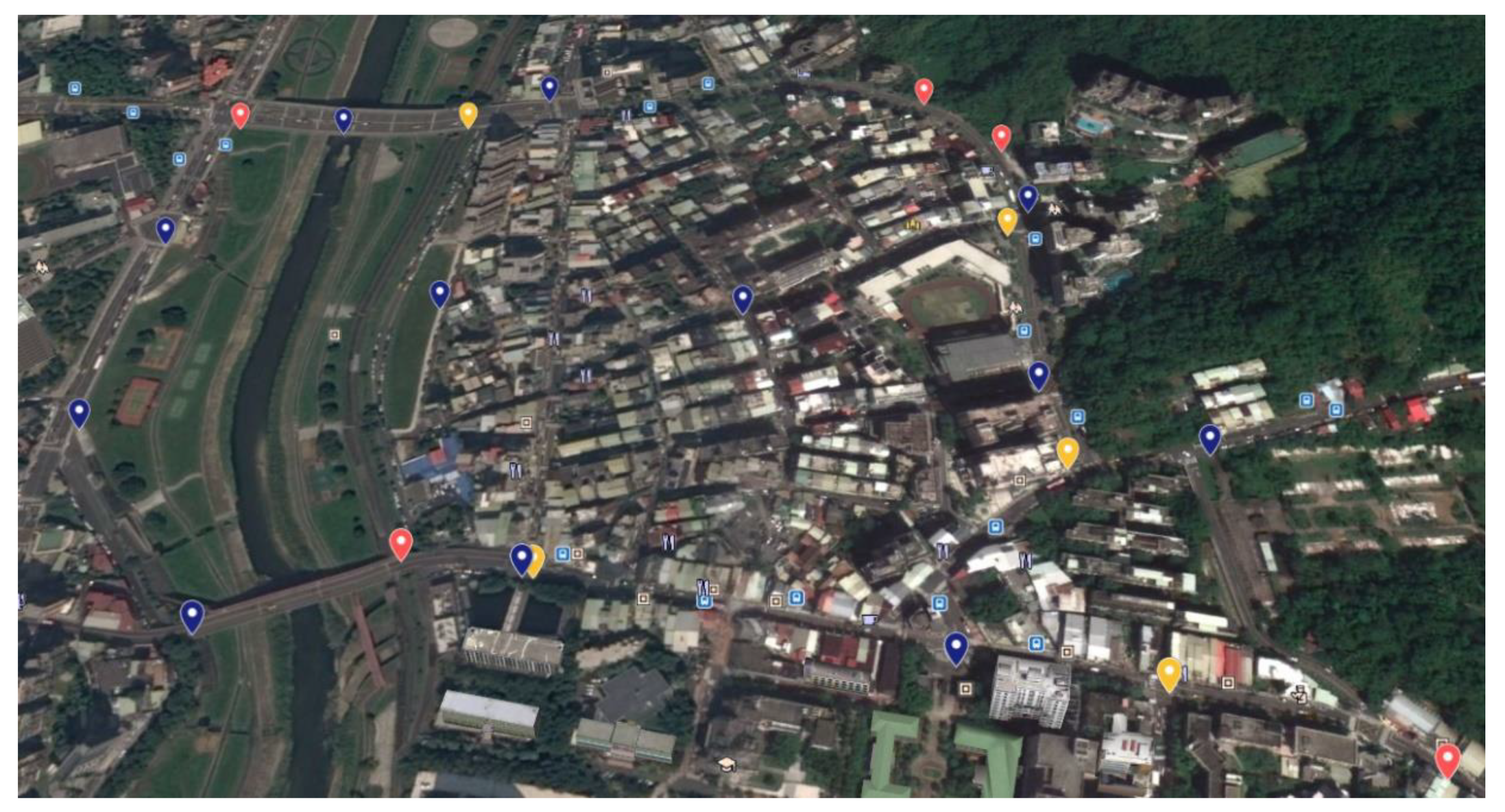
2.1.1. Planning and Dronestagramming

This study used the highly mobile AI-RIDER YJ-1000-HC multi-rotor UAV (performance shown in Table 1; devices shown in Figure 3a–c); and a PhaseOne iXU150 medium format camera, with a 55 mm fixed-focus lens shown in Figure 3d). The camera without a lens weighed 0.75 kg. Its image size was 8280 pixels × 6208 pixels, and the cell size was 5.3 microns, while the corresponding sensor size was 43.8 mm × 32.9 mm.
A UAV flight control computer was connected through the camera’s external shutter release. When the UAV reached the test area, the flight control computer triggered the camera to capture images and store them according to the flight plan. An AHRS (attitude and heading reference system), integrated with GPS signals, was installed on the drone. The flight control computer recorded the camera position by GPS and AHRS data, when each shot was triggered, for subsequent UAV aerial photogrammetric processing. The altitude was set to 300 m, and the ground resolution was set to about 3 cm in order to collect images and obtain high-precision aerial triangulation adjustment results economically. The waypoints were planned using a side-lap and end-lap of about 80% to reduce shadows and increase the visibility of objects and landmarks in order to more easily stereo-map more terrain details. Additionally, the dronestagramming range was expanded beyond the test area to ensure the quality and reliability of the UAV aerial photogrammetry.

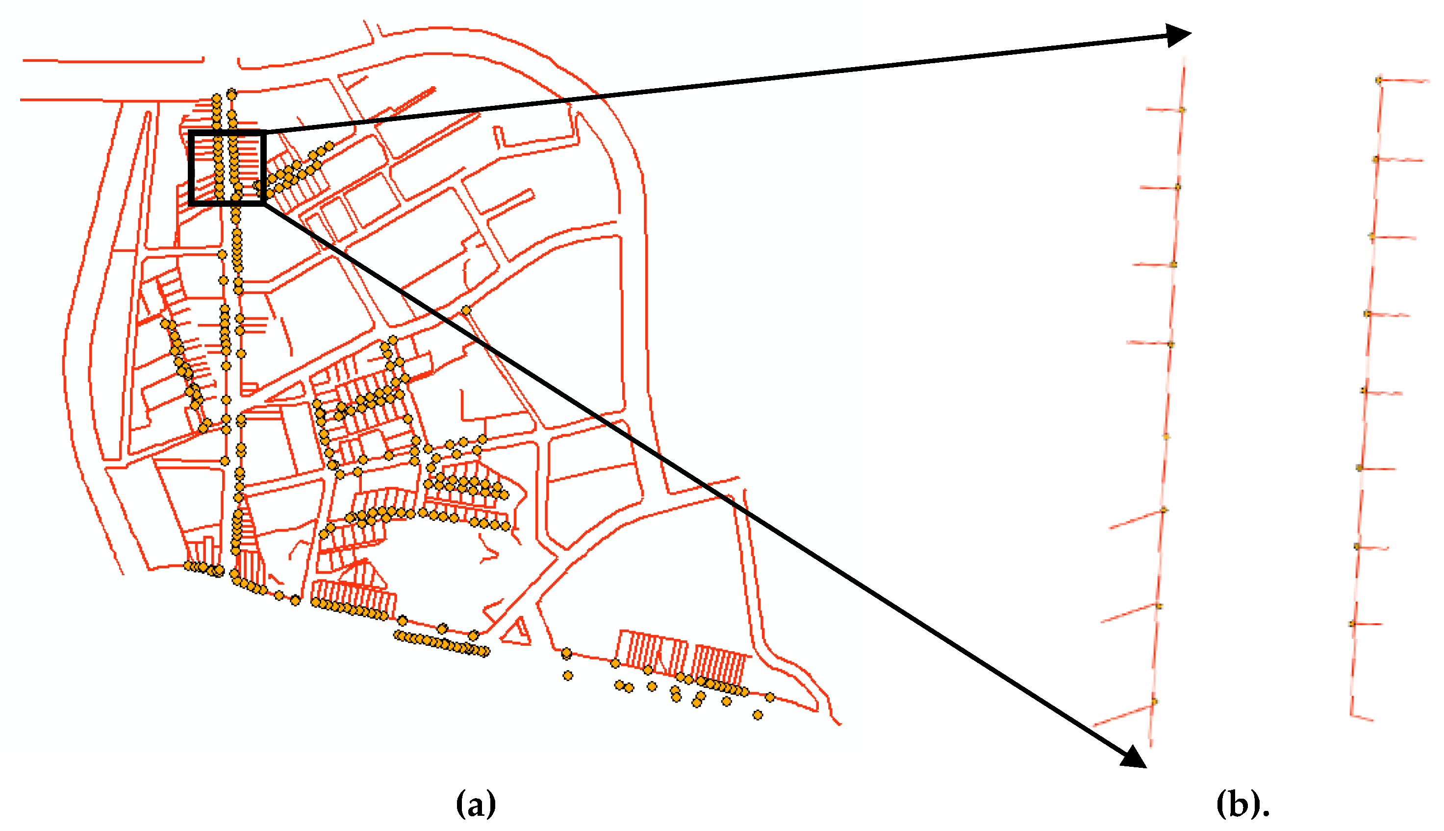
2.1.2. Setting and Surveying Aerial Photogrammetric Targets

Based on the Work Manual of One Thousand Digital Aerial Photogrammetric Topographical Maps in Urban Areas in Taiwan [13], more commonly known as the “Aerial Photogrammetric Work Manual”, the aerial photogrammetric targets in this study were set up at open locations. Meanwhile, the existing control points of the area were preferentially used as control points and checkpoints for aerial triangulation. Full control points were set up about 4~5 baselines from each other (baselines must be computed with a 60% image overlap).
Once the aerial photogrammetric targets were set, a material that was durable and had sufficient contrast with the ground color was selected for a clear identification and measurement. According to our experience, white painted squares could achieve the above-mentioned purpose. The size was designed based on the GSD (Ground Sampling Distance) of the images at about 3 cm, and the planned side length of the target was thus 20 cm. After imaging, the side consisted of about 6 pixels and could be clearly and easily identified in the image, shown in Figure 4.
Considering the accuracy, cost, and ease of operation, and with reference to the Handbook for Densified and Complementary Control Points with Virtual Base Station Real-Time Kinematic Positioning (VBS-RTK) Technology [14], VBS-RTK technology, called the e-GNSS survey in Taiwan, was used to determine the coordinates of the aerial photogrammetric targets in this study. e-GNSS is the name of the high-precision electronic global satellite real-time dynamic positioning system, constructed by the National Land Surveying and Mapping Center of the Ministry of the Interior, Taiwan. It is basically defined as the satellite real-time dynamic positioning system, based on Internet communication and wireless data transmission technology, in which the letter “e” means “electronic” and “networked”. GNSS stands for multi-satellite navigation and positioning systems (GPS + GLO + GAL + BDS + QZSS). If VBS-RTK was affected by poor mobile communication, and the original observation data were received from more than five satellites and with a PDOP (Position Dilution of Precision) value of less than 5, then OTF (On-The-Fly) post-processing was employed to determine the coordinates. The aerial photogrammetric targets were surveyed twice for averaging. Meanwhile, the differences in the horizontal position and elevation between the two surveys were not less than 3 cm and 5cm, respectively.
When e-GNSS was used to determine the coordinates of the aerial photogrammetric targets, the 3D coordinates of the locations with known announced control points in the cadastral coordinate system, surveyed using a ground survey by the Land Administration Bureau, Taipei City Government in Taiwan, were surveyed by a e-GNSS survey. The purpose was for the horizontal coordinate conversion to estimate and eliminate the systematic error between the cadastral coordinate system and e-GNSS coordinate system, while verifying the correctness of the coordinate conversion. Specifically, the eGNSS survey and least-squares collocation adjustment were used to obtain the cadastral coordinates of the aerial photogrammetric targets. Least-squares collocation is a combination of least squares adjustment, estimation, and filtering. Compared with the traditional adjustment method, which can only deal with random errors in observation [15], the least squares collocation method can also estimate the systematic error between two kinds of coordinates, namely, the cadastral coordinate system and the e-GNSS coordinate system, where observations were not made [16].
In this study, the TWD97 coordinate system was used for horizontal coordinates, and the TWVD2001 system was used for elevation. Therefore, the surveyed elevation was converted to the ortho-height system, according to the geoid model announced by the Ministry of the Interior (Taiwan).

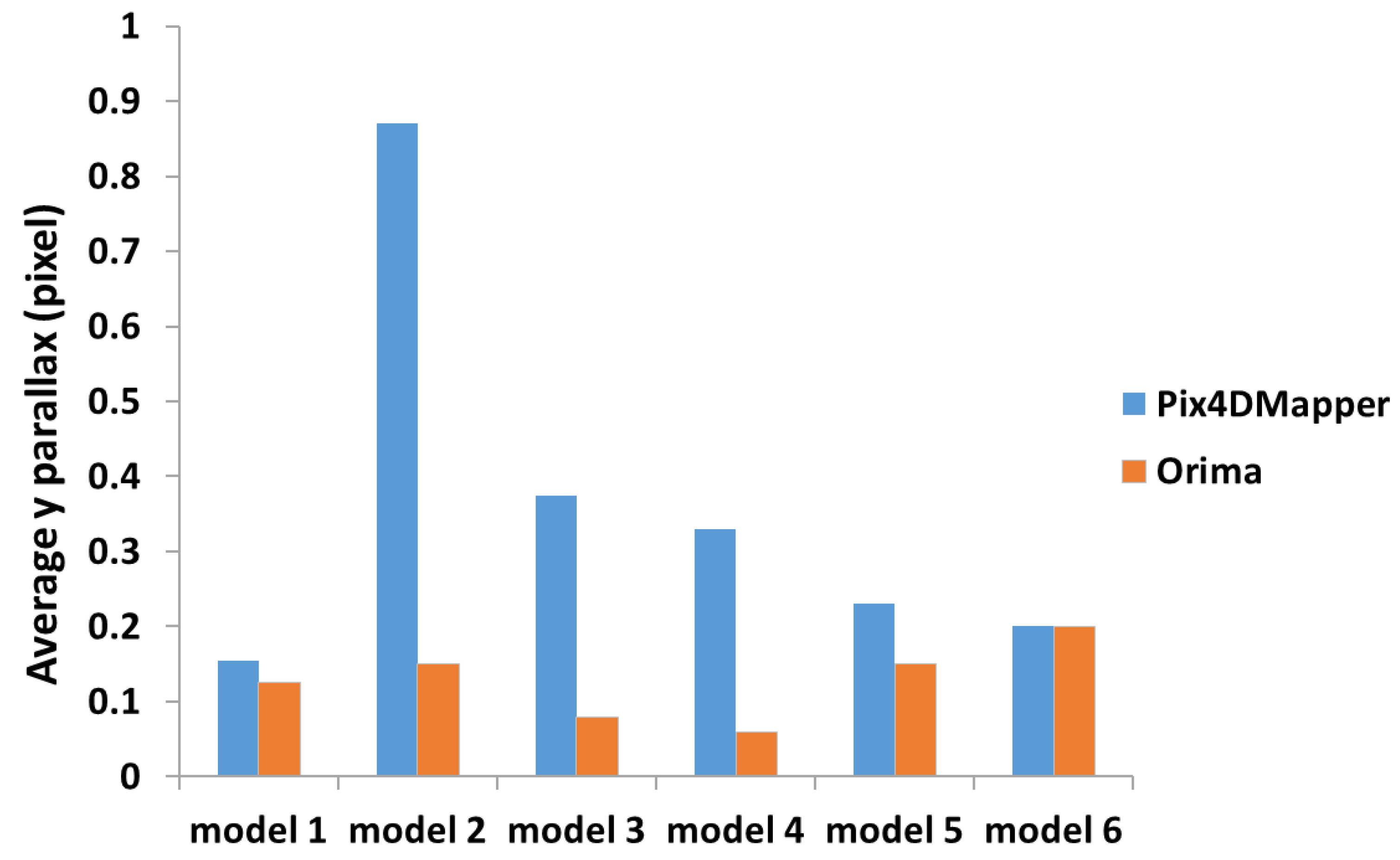
2.1.3. Aerial Triangulation (AT)

Once the UAV images were obtained, they were processed according to the AT work items described in the Aerial Photogrammetric Work Manual. The main processing steps of the self-calibration bundle adjustment include (1) the initial camera parameter inputs, (2) automatic tie point extraction, (3) free net adjustment, (4) automatic or manual blunder detection, (5) tie point manual measurement and deletion, (6) image point measurement of GCPs, and (7) self-calibration bundle adjustment for camera calibration.
Two AT results are presented and compared in this study. One was obtained using Pix4Dmapper [17], which is completely automated. The other was obtained using the Leica Photogrammetry Suite Orientation Management (ORIMA) [18] photogrammetric software, a conventional semi-automatic software for AT in aerial photogrammetry. Both AT processing procedures were implemented using the self-calibration bundle adjustment [19], which can not only determine the exterior parameters of images, but also the camera parameters, including the principal focal length, principal point location and system errors from lens or film distortions. This means that the basic collinearity equation is augmented by the additional terms, Δx and Δy. The Δx and Δy terms consist of various additional parameters based on different models. The camera model or camera parameters used by the Pix4Dmapper is as shown in Equations (1)–(4), and the output unit of the camera parameters is pixels [17].
x d = x ( 1 + d r + d t x ) O o a y d = y ( 1 + d r + d t y )
d r = r 3 R 1 + r 5 R 2 + r 7 R 3
d t x = 2 t 1 x y + t 2 ( r 2 + 2 x 2 )
d t y = 2 t 2 x y + t 1 ( r 2 + 2 y 2 )
where ( x d , y d ) : the image coordinates after correcting the lens distortion. ( x , y ) : the image coordinates before correcting the lens distortion. R 1 ~ R 3 : the radial parameters of the lens distortion. t 1 ~ t 2 : the decentering parameters of the lens distortion. r = x 2 + y 2 : the radial distance.
The ORIMA photogrammetric software for AT adapts the Brown physical model. Equation (5) shows the Brown mathematical model, which was originally developed for frame camera calibration.
Δ x = x 0 + x [ a 1 ( r 2 r 0 2 ) + a 2 ( r 4 r 0 4 ) + a 3 ( r 6 r 0 6 ) ] + b 1 x + b 2 y                           + x c [ c 1 ( x 2 y 2 ) + c 2 x 2 y 2 + c 3 ( x 4 y 4 ) ] + d 1 x y + d 2 y 2 + d 3 x 2 y + d 4 x y 2 + d 5 x 2 y 2 Δ y = y 0 + y [ a 1 ( r 2 r 0 2 ) + a 2 ( r 4 r 0 4 ) + a 3 ( r 6 r 0 6 ) ]                           + y c [ c 1 ( x 2 y 2 ) + c 2 x 2 y 2 + c 3 ( x 4 y 4 ) ] + d 6 x y + d 7 x 2 + d 8 x 2 y + d 9 x y 2 + d 10 x 2 y 2
where, Δ x , Δ y : the corrected image point coordinate observations; x 0 , y 0 : the principal point coordinates; c: the calibrated focal length; r , r 0 : the radial distance from the measurement point to the image center and principal point, respectively; a 1 , a 2 , a 3 : the radial lens distortion polynomial coefficients; b 1 , b 2 : the affinity and non-orthogonality of the image system; c 1 , c 2 , c 3 : the unflatness of the image plane; d 1 d 10 : the regular and irregular film deformations.
When ORIMA was used, AT was performed using the free-net and constraint bundle adjustment first, while the final solution was solved by the self-calibration bundle adjustment. In self-calibration bundle adjustment, the high correlation, significance and determinability of the self-calibration parameters were carefully analyzed, and then appropriate parameters were selected for the final adjustment. However, Pix4Dmapper is automated, so these issues in the ORIMA software were not considered. Meanwhile, five checkpoints were selected for each AT result to verify the AT accuracy.

2.1.4. Supplementary Control Point Measurements for the Boundary Verification Survey

After AT, this study discusses two approaches to obtaining supplementary control point coordinates for boundary verification. Because the Pix4Dmapper software has a user-friendly interface and function for measuring the coordinates by space intersection using multiple bundles, it was used in this study to measure the coordinates of supplementary control points (Figure 5). In the first approach, the coordinates of supplementary control points were measured using the AT results directly from Pix4Dmapper. In the second approach, the coordinates of supplementary control points were measured using the AT results from ORIMA. The reason is the AT results obtained from ORIMA are more suitable for stereo-mapping. An advanced discussion will be presented in Section 3.1.5 using the approach described in Section 2.1.5. Because the camera parameters adopted by ORIMA and Pix4Dmapper are different (see Equations (1)–(5)), as described in Section 2.1.3, the camera parameters of ORIMA cannot be imported into Pix4Dmapper. Therefore, the second approach should firstly obtain the undistorted images by resampling the original images based on the calibrated camera parameters, and then all the undistorted images, including the exterior parameters and pixel size, can be imported into Pix4Dmapper to measure the supplementary control point coordinates (see Figure 5). For comparison, the coordinates of the same supplementary control points were surveyed in the cadastral coordinate system using a total station by the Land Administration Bureau, Taipei City Government in Taiwan. After the tests described in Section 2.1.5, the approach with the best results was chosen to provide supplementary control coordinates for boundary verification.

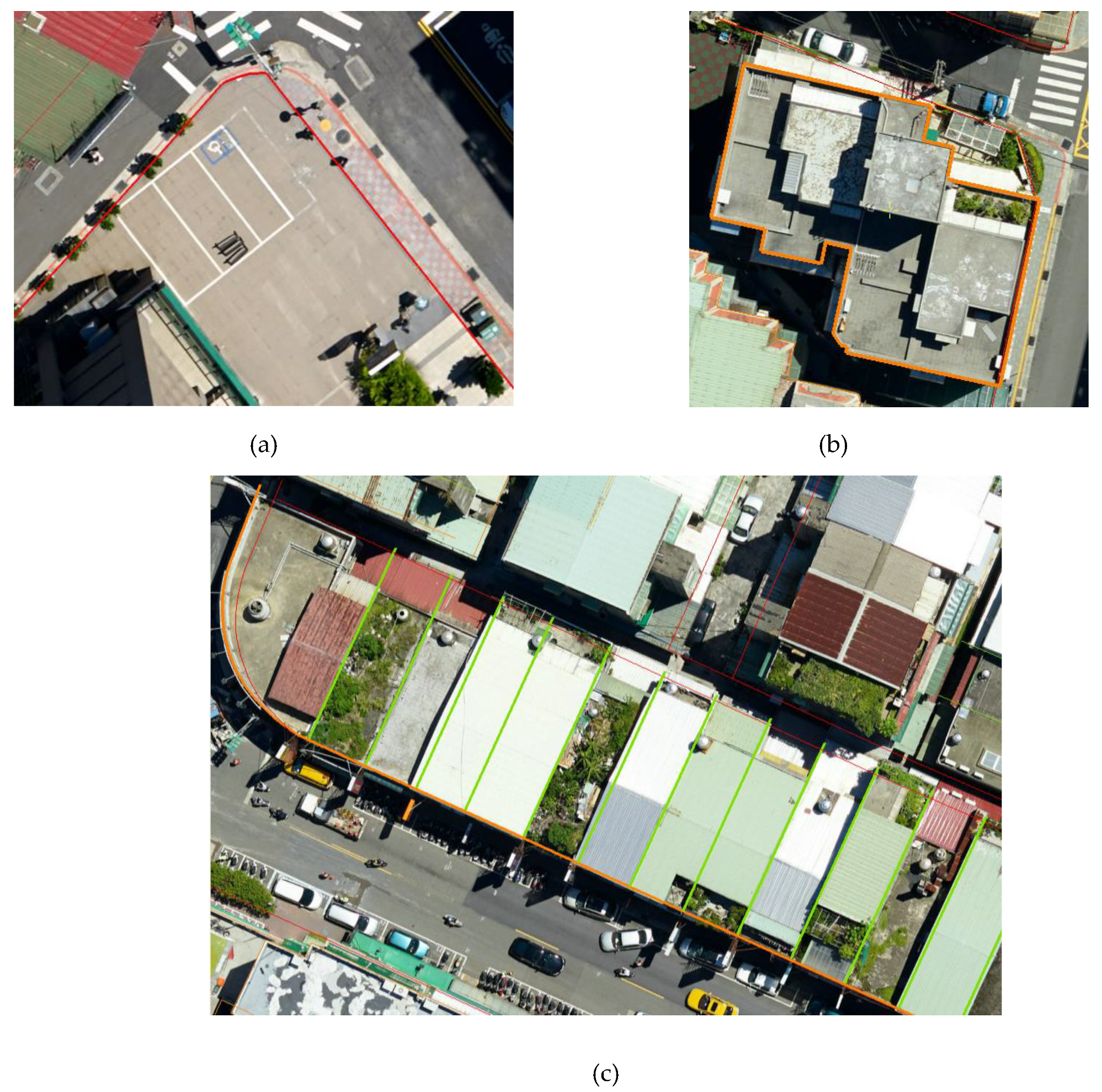
2.1.5. Detailed Map Generation by UAV Aerial Photogrammetric Stereo-mapping

A detailed survey measures the coordinates of topographic detail points that are possible locations of parcel lines, including the parcel corners. The purpose of a detail survey is to provide possible parcel points, including the possible parcel corners or parcel points on the parcel boundary, for map registration, after the overlap analysis of the possible parcel points and the digitalized graphic cadastral map, in order to identify the coordinates of the parcel corners for boundary verification. UAV aerial photogrammetry was used in this study to globally measure the terrain detail points to conduct a global overlap analysis in order to perform map registration and further confirm the consistency between the digitized cadastral map and current actual land details in the TWD97 coordinate system. This method is unlike a traditional ground detail survey for boundary verification, in which only local detail points are surveyed, meaning there will only be local consistency between a cadastral map and land details. The abovementioned detail points are usually located on the boundary of natural terrain features (such as ridges, valleys, waterways, etc.) or artificial features (such as ditches, road boundaries, ridge footpaths, embankments, or crop boundaries). In a detail survey using UAV aerial photogrammetry, the 3D cadastral lines were generated and overlapped on stereo models in order to obtain references to stereo-map the positions of the detail points near the parcel lines. The elevation of the 2D cadastral lines was interpolated from DSM (Digital Surface Model) data, generated from the dense matching of UAV images, to form 3D cadastral lines.
The principle of stereo mapping is derived from the principles of field surveying in subsection 807 of the Resurvey Handbooks of Cadastral Maps by the Digital Method in Taiwan. Moreover, based on the characteristics of digitalized graphic urban cadastral maps in Taiwan, urban terrain details were stereo-mapped to identify possible parcel points on the parcel boundaries, for example, (1) road boundaries (Figure 6a); (2) the centerline of a wall on the top of a building of the same style, except for the wall on the outermost boundary of the top of the building; (3) the outer edge of a wall on the outermost boundary of the top of a building of the same style (red lines in Figure 6c), and the outer edge of a wall of a single building (red lines in Figure 6b), except the wall attached to exposed steel reinforcing; (4) roof eaves (green lines in Figure 6c); (5) an embankment within the scope of a waterway and bounded by the lower foot of its embankment; and (6) the location of changes of vegetation covers and topographical change boundaries.
Because two AT results were obtained from ORIMA and Pix4Dmapper, one must be chosen for detailed map generation by stereo-mapping. Because y parallax in the stereo model will cause discomfort during stereo-mapping, six well-distributed models were selected for the comparison of the y parallax of the two AT results. Six evenly distributed checkpoints in each model verified the y parallax. The method for checking the y parallax involves stereoscopic observation and then splitting the model into left and right images, as shown in Figure 7. The difference between a floating mark in the left and right images in the y direction are measured as the y parallax. Each checkpoint was observed and measured 3 times to average the results. The stereoscopic observation was performed using the PRO600 software. PRO600 is an integrated suite of software applications from Hexagon Geospatial, which optimizes MicroStation for photogrammetric vector data collection and editing.
The AT result with the smallest y parallax was used to generate a detailed map and orthoimage using the Pix4Dmapper software. The detailed map generated by UAV aerial photogrammetry was then compared with the one surveyed by ground surveying using a total station.

2.2. Survey for the Boundary Verification of a Digitalized Cadastral Area of Taiwan

2.2.1. Map Registration

Map registration is performed after overlapping the detailed map and generating orthoimage with digitized cadastral maps. The goal of map registration is to identify the relationship between the digitized cadastral maps and actual terrain details. Thus, the relationship between digitalized cadastral maps and current land detail situations should be as consistent as possible, thus increasing the reliability and accuracy of the digitized cadastral map. Before map registration, area partitions are used to divide all the digitalized graphic cadastral areas into several subareas. This makes them compatible with affine transformation, with a different scale factor for each axis, in ArcMap software to absorb errors, including map shrinkage and deformation, and it also allows them to better fit with the cadastral maps and the actual land details in the TWD97 coordinate system. Once the partitions were determined, the suitable and evenly distributed points between the digitalized cadastral maps and current land detailed maps in each subarea were selected for affine transformation. Then, before and after map registration, the vertical distances from the detail points to the cadastral lines in each subarea were calculated to determine whether the actual land details were consistent with the cadastral maps.

2.2.2. Survey for Boundary Verification

In this stage, the coordinates of the supplementary control points were measured for boundary verification by the space intersection of multiple bundles in UAV aerial photogrammetry, and the measurement tool is the same as that shown in Figure 5. The computed horizontal distances and angles among the measured coordinates of the supplementary control points and the measured coordinates of the parcel points from the cadastral map were used to stake out the parcel points in the real world by the radiation or free station method using a total station. The radiation method using a total station is the most usual method for verification surveys. The total station was set up on the control point. Then, the parcel points were verified by the computed horizontal distance and angle. The free station method using a total station set up the total station where it could see the control points and parcel points. At this moment, the total station was not set up on the control point. The free station method is more convenient than the radiation method, but the coordinates of the free station have to be determined after observing at least two control points. Meanwhile, the desired horizontal distances and angles among the control points and the parcel points have to be calculated on site. If the observation sight among the control points and parcel points is clear, the radiation method using a total station is recommended. The results of the boundary verification survey presented in this study were checked according to Articles 75 and 76 of the Regulations for the Implementation of Cadastral Surveys in Taiwan.

3. Results and Discussion

The following sections will present the test results. The first section gives the UAV aerial photogrammetry results, and the second gives the boundary verification survey results.

3.1. UAV aerial Photogrammetry

3.1.1. Planning and Dronestagramming

Based on the plan, it was estimated that 250 images would be taken (see the designed waypoints in Figure 8). However, only 230 images were actually collected. The final dronestagramming locations by UAV are shown as red points in Figure 9. In addition, the blue “+” marks indicate the control and checkpoints for AT, and the yellow circles indicate the models selected for the stereoplotting test described in Section 3.1.4.

3.1.2. Setting and Surveying of Aerial Photogrammetric Targets

Using the principles of control point selection described in Section 2.1.2, Figure 10 demonstrates 16 control points (red and blue marks) and 5 checkpoints (yellow marks), where the red marks are the 5 announced control points that are also used for the subsequent least squares collocation in the next step to confirm the consistency of the coordinate reference system between the cadastral map system and e-GNSS coordinate system. The relationship between all control points and dronestagramming locations is shown in Figure 9.
The TWD97 coordinates of 21 aerial photogrammetric targets were obtained after two e-GNSS surveys of each target. The maximum difference of the horizontal position and elevation between two e-GNSS surveys were 2.9 cm and 2.7 cm, respectively. This meets the requirements and subsequent least squares collocation based on the affine transformation of the five announced control points (red marks shown in Figure 10) to confirm the consistency of the coordinate reference system. The results of the least squares collocation are shown in Table 2. GA0476, GA0477, GA0494, 100010 and QT79 were the five announced control points. Ntran (m) and etran (m) indicated the (N, E) coordinates before the least squares collocation, and ninterp (m) and einterp (m) showed the (N, E) coordinates after the least squares collocation. Ndef (m) and edef (m) were the system error between the cadastral coordinate system and e-GNSS coordinate system. The system error between the cadastral coordinate system and e-GNSS coordinate system for the five announced control points was not so obvious, because the maximum error was −0.009 m in the E coordinate component at Point No. 10010.
After the least squares collocation, the ratio of the distance difference between any two points was calculated for analysis. The maximum ratio of the distance difference between any two points (baseline) was 1/21535, which meets the 1/5000 requirement of the Handbook for Densified and Complementary Control Points with Virtual Base Station Real-Time Kinematic Positioning (VBS-RTK) Technology [14]. The obtained coordinates after the least squares collocation, based on affine transformation, were also verified by the horizontal distances measured by a total station. Table 3 shows the check results. The maximum relative ratio of the distance difference for five ground surveyed horizontal distances was 1/3335, which meets the 1/3000 requirement of the Handbook for Densified and Complementary Control Points with Virtual Base Station Real-Time Kinematic Positioning (VBS-RTK) Technology [14].

3.1.3. Aerial Triangulation (AT)

As mentioned in Section 2.1.3, two AT results are presented and compared in this study. One was obtained using Pix4Dmapper, which is completely automated. The other was obtained using the ORIMA photogrammetric software, a conventional semi-automatic software package for AT in aerial photogrammetry. Pix4Dmapper is automated, and the camera parameters, after automatic self-calibration, are shown in Table 4. While using the ORIMA software, the high correlation, significance, and determinability of the self-calibration parameters were carefully analyzed, and then the final appropriate parameters were selected for the final adjustment. The calibrated camera parameters are tabulated in Table 5, indicating that radial lens distortion was the main error source. A comparison of the camera parameters determined by self-calibration from Pix4Dmapper and ORIMA would be meaningless, because the camera model adopted by Pix4Dmapper and ORIMA is different (see Equations (1)–(5)). Thus, it was difficult to compare the camera parameters determined by these two software packages. Therefore, the same checkpoints were used to analyze the AT results. The AT check results, obtained using Pix4Dmapper and ORIMA, are shown in Table 6. In Table 6, the RMSE (Root Mean Square Error) values of the checkpoints for the Pix4Dmapper result were 0.0087 m in the E direction and 0.0110 m in the N direction, while the RMSE values of the checkpoints for the ORIMA result were 0.0103 m in the E direction and 0.0091 m in the N direction. Neither result exhibits a significant difference. This indicates a high-quality camera calibration. In particular, the camera parameters calibrated by ORIMA were only the focal length (f), principal point coordinates (x0, y0), and radial lens distortion (a1, a2, a3), after the high correlation, significance, and determinability of the self-calibration parameters were carefully analyzed.

3.1.4. Measurements of the Supplementary Control Points for the Boundary Verification Survey

Six announced control points were selected for comparison in the tests for the measurements of supplementary control points for the boundary verification survey using UAV aerial photogrammetry. The six announced control points are shown as the cyan-blue pin marks in Figure 11. After aerotriangulation, the difference analyses of the two compared coordinate methods are tabulated in Table 7. Table 7 shows that the RMSE of the E coordinate differences were 0.005 m and 0.006 m, and the RMSE of the N coordinate differences were 0.008 m and 0.011 m. The results of the two methods are thus almost the same.

3.1.5. Detailed Map of UAS Aerial Photogrammetric Stereo Mapping

This subsection presents the detailed map results achieved using stereo-mapping. As mentioned in Section 2.1.5, two AT results were obtained, and one was chosen for detailed map generation by stereo-mapping. Six well-distributed models (see the yellow ovals in Figure 9) were selected for a comparison of the y parallax in these two AT results, and there were six evenly distributed checkpoints in each model. The result is shown below in Figure 12, in which the average y parallax values are all less than 1 pixel in the six models from the two AT results, and the ORIMA AT result had a smaller y parallax value to that achieved by Pix4Dmapper. The average y parallax of all points in the six models was 0.36 pixels using the AT results from Pix4Dmapper and 0.13 pixels using the AT results from ORIMA. All the y parallax values in model 1, 3, 4, 5, 6 in six locations of each model were less than 1 pixel, except for model 2. A y parallax value larger than 1 pixel will cause discomfort while stereo-mapping. Figure 13 shows a comparison of the y parallax for six locations in model 2, and the y parallax is larger than 1 pixel at points 2 and 5. This means that stereo-mapping using the Pix4Dmapper AT result may cause discomfort. The reason is that while the AT for the Pix4Dmapper was fully automatic, some incorrect tie points were not completely removed. Based on the above analysis, this study used the AT result of ORIMA to generate the detailed map manually, and the orthoimage automatically by Pix4Dmapper. The results are shown in Figure 14. Meanwhile, the coordinate measurement of the supplementary control points for the boundary verification survey also used the ORIMA AT results. According to the computed camera parameters, the undistorted images were resampled from the original images. These undistorted images, including the exterior parameters and pixel size, were imported into Pix4Dmapper to measure the coordinates of the supplementary control points by space intersection using multiple bundles of the tool, as shown in Figure 5.
A comparison of the detailed map surveyed by ground surveying and UAV aerial photogrammetry is shown in Figure 15a. Local enlargement is demonstrated in Figure 15b. The red lines define the detailed map stereo-mapped by UAV aerial photogrammetry, and the orange points are the points of the detailed map surveyed by a total station. It is clear that the detailed map stereo-mapped by UAV aerial photogrammetry includes much more detailed data than the details obtained by a total station, which could only collect data near roads. As shown in Figure 15b, there is no difference between the two kinds of data by visual verification. Quantity verification was conducted using the vertical distances from the points surveyed by a total station to the lines of the detailed map stereo-mapped by UAV aerial photogrammetry. The result is demonstrated in Figure 16. For the comparison, 187 detail points were surveyed. There were 77 points at a distance of less than 10 cm, 73 points between 10 and 20 cm, and 28 points between 20 to 30 cm, while only 9 points were over 30 cm apart. Most of the distance differences were less than 20 cm. This shows that the detailed map data using UAV aerial photogrammetry are suitable for the map registration of digitalized graphic maps with a 1/500 map scale. The difference between the two kinds of data was due to the identification of possible parcel points. The ground survey identified them on the ground, while UAV photogrammetry identified them from the stereo model, which is effectively from the sky. Even the identification was quite different; 77 points at a distance of less than 10 cm meant that the ground survey and UAV aerial photogrammetry were consistent.

3.2. Survey for the Boundary Verification of a Digitalized Cadastral Area of Taiwan

3.2.1. Map Registration

Before the boundary verification survey, map registration must be performed, as described in Section 2.2.1, in order to identify the coordinates of the parcel points for boundary verification. Based on the street layout, 11 subareas, as shown in the left of Figure 17, were partitioned. Figure 18 shows that the average distance difference in most areas is more than 15 cm, with the exception of areas A, G, and H, before map registration. After map registration with affine transformation in each subarea, the average distance difference in each area is reduced by 2 to 9 cm, and all values were less than 15 cm (see the red bars in Figure 18). After each subarea was transformed using affine transformation, and all subareas were merged into one cadastral map (see the right of Figure 17), which was the final version of the boundary verification survey.

3.2.2. Boundary Verification Survey

In a boundary verification survey, surveyors must stake out the parcel points according to the computed horizontal distances and angles from the coordinates of the parcel points in a cadastral map and the coordinates of the control points. This study used building corners and ground road corners as supplementary control points, and their coordinates were determined by space intersection from multiple bundles of UAV aerial photogrammetry. The parcel points were also staked out by the radiation method or free station method using a total station. The radiation method using a total station is the most common methodology for verification surveys. The total station was set up on the control point. Then, the parcel points were verified by the computed horizontal distance and angle. The free station method using a total station set up the total station where it could see the control points and parcel points. At this moment, the total station was not set up on the control point. The free station method is more convenient than the radiation method, but the coordinates of the free station have to be determined after observing at least two control points. Meanwhile, the desired horizontal distances and angles among the control points and the parcel points have to be calculated on site.
The test area is shown in Figure 19, where S is the surveying station and points 1–6 are the parcel points for the boundary verification survey. The ground road corners selected as supplementary control points are shown in Figure 19a, and the building corners used as supplementary control points are shown in Figure 19b. According to the Regulations for the Implementation of Cadastral Surveys in Taiwan, the difference between the surveyed and computed horizontal distance from a supplementary control point to the parcel point must be less than 0.3 mm in the cadastral map coordinates, where the surveyed horizontal distance was measured by a total station, and the computed horizontal distance was calculated from the 2D coordinates of a supplementary control point to the 2D coordinates of the parcel point. Because the map scale is 1/500, the distance difference between the surveyed and computed horizontal distance must be less than 0.15 m in the object space after the boundary verification survey. In addition, the difference between the computed horizontal distance between the coordinates of adjacent parcel points in a cadastral map and the horizontal distance measured by a ground survey should satisfy the following formula:
4   cm + 1   cm L + 0.02   cm M
where L is the horizontal distance, the measurement unit is meters, and M is the map scale denominator. The horizontal distance between adjacent parcel points for verification is about 5 m (see “Computed horizontal distance” fields in the right part of Table 8), and the difference threshold of each side must therefore be less than 0.162 m after the boundary verification survey. The result is shown in Table 8, in which all of the results meet the required standards. Specifically, using building roof corners as controls is feasible and makes a boundary verification survey more flexible, even though it is more difficult to find suitable corners as controls.
The parcel points after a boundary verification survey using road corners as controls, staked out by the free station method, are shown in Figure 20. The locations after the verification staking survey were located at the centers of walls, indicated by the red arrows, and are consistent with the cadastral reconnaissance data. This demonstrated the feasibility of a boundary verification survey using a detailed map and orthoimage generated by UAV aerial photogrammetry in digitalized urban cadastral areas.

4. Conclusions

In this study, the feasibility of a boundary verification survey using UAV aerial photogrammetry in a digitalized urban cadastral area of Taiwan was investigated. A high-quality-medium format camera, with a 55 mm focal length, was carried on a rotary UAV to record 3 cm GSD (ground sampling distance) images, flying at an altitude of 300 m. The images were taken with an 80% end-lap and side-lap to increase the visibility of more terrain details for stereo-mapping. While the AT results from the Pix4Dmapper and ORIMA software were almost the same, the y parallax from the AT result achieved using the ORIMA software was lower than that achieved using Pix4Dmapper. Therefore, the detailed map was produced by the AT achieved using ORIMA. According to the test conducted in this study, UAV aerial photogrammetry can generate many more land detail points globally, i.e., more detailed maps, and orthoimages for map registration, ensuring that the resulting digitalized cadastral maps are much more consistent with the collected possible parcel points after map registration. In the map registration stage, after determining 11 partitions for map registration in order to absorb errors using affine transformation, the distance differences were reduced by 2-9 centimeters in different partitions after map registration. After this, the coordinates of the parcel points for the verification survey were obtained after map registration. Additionally, UAV aerial photogrammetry provided the coordinates of the supplementary control points using the AT result from ORIMA. Then, all the resampled undistorted images based on the computed camera parameters, including the exterior parameters and pixel size, were imported into the Pix4Dmapper software to measure the coordinates of the supplementary control points by space intersection using multiple bundles (see Figure 5). Finally, the distance and angle between the parcel points of the verification and supplementary control points were calculated for the boundary verification survey by the radiation method using a total station. Even the building corners were used as controls for the boundary verification survey by the free station method, using a total station to complete the boundary verification survey process. The results all met the standards required by the Regulations for the Implementation of a Cadastral Survey, art. 75 and art. 76, in Taiwan. This proved the feasibility of a boundary verification survey using UAV aerial photogrammetry in digitalized urban cadastral areas. Simultaneously, the proposed approach was able to generate one cadastral map that was consistent with the actual terrain details, meaning that while boundary verification surveys are necessary, surveyors do not need to locally survey the terrain represented in the detailed map. Therefore, the proposed approach can reduce labor costs and improve the efficiency of future boundary verification surveys.

Author Contributions

S.-H.C. conceived and designed the experiments; S.-H.C. and C.-C.C. together performed the test, analyzed the data, and wrote the paper. All authors have read and agreed to the published version of the manuscript.

Funding

This research received no external funding.

Acknowledgments

A special thanks is extended to AI-RIDER Corp for the UAS. The detail surveying data from ground surveys were provided by the Land Development Agency, Department of Land Administration, Taipei City Government, Taiwan (R.O.C). The detailed map was produced by YuDa Co. Ltd. The authors would also like to thank their supporters.

Conflicts of Interest

The supporters had no role in the design of the study, in the analyses, or interpretation of data, in the writing of the manuscript, nor in the decision to publish the results.

References

  1. Wu, T.P.; Kao, S.P.; Ning, F.S. Study on Computer Registering for Land Revision of Digitialized Graphic Maps. J. Cadastr. Surv. 2003, 22, 1–23. (In Chinese) [Google Scholar]
  2. Eisenbeiss, H. A mini Unmanned Aerial Vehicle (UAV): System overview and image acquisition. Int. Arch. Photogramm. Remote Sens. 2004, XXXVI-5/W1, 36, unpaginated CD-ROM. [Google Scholar]
  3. Berni, J.; Zarco-Tejada, P.; Suárez, L.; Fereres, E. Thermal and narrowband multispectral remote sensing for vegetation monitoring from an unmanned aerial vehicle. IEEE Trans. Geosci. Remote Sens. 2009, 47, 722–738. [Google Scholar] [CrossRef] [Green Version]
  4. Lin, Y.; Hyyppä, J.; Jaakkola, A. Mini-UAV-Borne LIDAR for Fine-Scale Mapping Geoscience and Remote Sensing Letters. IEEE Trans. Geosci. Remote Sens. 2011, 8, 426–430. [Google Scholar] [CrossRef]
  5. Lerma, J.; Navarro, S.; Cabrelles, M.; Villaverde, V. Terrestrial laser scanning and close range photogrammetry for 3D archaeological documentation: The Upper Palaeolithic cave of Parpall as a case study. J. Archaeol. Sci. 2010, 37, 499–507. [Google Scholar] [CrossRef]
  6. Reich, M.; Wiggenhagen, M.; Muhle, D. Filling the holes—Potential of UAV-based photogrammetric facade modeling. In Proceedings of the Tagungsband des 15, 3D-NordOst Workshops der GFaI, Berlin, Germany, 6–7 December 2012. unpaginated CD-ROM. [Google Scholar]
  7. Mesas-Carrascosa, F.; Rumbao, I.; Berrocal, J.; Porras, A. Positional Quality Assessment of Orthophotos Obtained from Sensors Onboard Multi-Rotor UAV Platforms. Sensors 2014, 14, 22394–22407. [Google Scholar] [CrossRef] [PubMed]
  8. Remondino, F.; Barazzetti, L.; Nex, F.; Scaioni, M.; Sarazzi, D. Uav photogrammetry for mapping and 3d modeling-current status and future perspectives. Int. Arch. Photogramm. Remote Sens. Spat. Inf. Sci. 2011, 38, C22. [Google Scholar] [CrossRef] [Green Version]
  9. Ahmad, A. Digital Mapping Using Low Altitude UAV. Pertanika J. Sci. Technol. 2011, 19, 51–58. [Google Scholar]
  10. Manyoky, M.; Theiler, P.; Steudler, D.; Eisenbeiss, H. Unmanned aerial vehicle in cadastral applications. In Proceedings of the International Archives of the Photogrammetry, Remote Sensing and Spatial Information Sciences, ISPRS Zurich 2011 Workshop, Zurich, Switzerland, 14–16 September 2011; Volume XXXVIII-1/C22. [Google Scholar]
  11. Rijsdijk, M.; van Hinsbergh, W.H.M.; Witteveen, W.; ten Buuren, G.H.M.; Schakelaar, G.A.; Poppinga, G.; van Persie, M.; Ladiges, R. Unmanned aerial systems in the process of juridical verification of cadastral border. Remote Sens. Spat. Inf. Sci. 2013, 11, W2. [Google Scholar] [CrossRef] [Green Version]
  12. Crommelinck, S.; Bennett, R.M.; Gerke, M.; Yang, M.Y.; Vosselman, G. Contour Detection for UAV-Based Cadastral Mapping. Remote Sens. 2017, 9, 171. [Google Scholar] [CrossRef] [Green Version]
  13. Work Manual of One Thousandth of Digital Aerial Photogrammetric Topographical Maps in Urban Area; Ministry of the Interior: Taipei City, Taiwan, 2010. (In Chinese)
  14. Handbook for Densified and Complementary Control Points with Virtual Base Station Real Time Kinematic Positioning (VBS-RTK) Technology; Land Surveying and Mapping Center, Ministry of the Interior, Ministry of the Interior: Taipei City, Taiwan, 2010.
  15. Moritz, H. Advanced Least-Squares Methods; Reports of the Department of Geodetic Science; The Ohio State University: Columbus, OH, USA, 1972; NO.175. [Google Scholar]
  16. Ruffhead, A. An introduction to least-squares collocation. Surv. Rev. 1987, 29, 85–94. [Google Scholar] [CrossRef]
  17. Pix4Dmapper Software Manual. Retrieved from Taiwan on the World Wide Web. Available online: https://support.pix4d.com/hc/en-us/articles/202558109-Pix4Dmapper-Software-Manual-Index-View (accessed on 28 August 2019).
  18. Erdas, I.N.C. LPS Project Manager User’s Guide; Erdas Inc.: Norcross, Georgia, 2008. [Google Scholar]
  19. Wolf, P.R.; Dewitt, B.A. Elements of Photogrammetry: With Applications in GIS, 3rd ed.; McGraw-Hill Publisher: New York, NY, USA, 2000. [Google Scholar]
Figure 1. Study flowchart.
Remotesensing 12 01682 g001
Figure 2. Test area (in red polygon).
Remotesensing 12 01682 g002
Figure 3. AI-RIDER YJ-1000-HC Multi-Rotor UAV and PhaseOne iXU150 Camera. (a) Body; (b) Remote controller; (c) Ground control station; (d) Camera.
Remotesensing 12 01682 g003
Figure 4. Diagrams of the square aerial photogrammetric targets. (a) Example 1 of square targets; (b) Example 2 of square targets; (c) Local enlargement of example 1; (d) Local enlargement of example 2.
Remotesensing 12 01682 g004aRemotesensing 12 01682 g004b
Figure 5. The interface for measurements of supplementary control points.
Remotesensing 12 01682 g005
Figure 6. Illustration of urban terrain details for stereo-mapping to identify possible parcel points: (a) road boundaries (red lines), (b) outer edge of a wall of a single building (red lines), and (c) the outer edge of a wall on the outermost boundary (red lines) and roof eaves (green lines).
Remotesensing 12 01682 g006
Figure 7. Schematic diagram for y parallax measurement.
Remotesensing 12 01682 g007
Figure 8. Planned waypoints for dronestagramming.
Remotesensing 12 01682 g008
Figure 9. Final dronestagramming locations. (Red points: actual dronestagramming locations; Blue “+”: control and checkpoints for AT; Yellow ovals: models selected for the stereoplotting test.).
Remotesensing 12 01682 g009
Figure 10. The locations of the control points and checkpoints (control points: red and blue marks; checkpoints: yellow marks).
Remotesensing 12 01682 g010
Figure 11. The distribution of the six announced control points.
Remotesensing 12 01682 g011
Figure 12. Average y parallax comparison results for two AT results.
Remotesensing 12 01682 g012
Figure 13. The y parallax in six locations of model 2.
Remotesensing 12 01682 g013
Figure 14. Left: the stereo-mapped detailed map; Right: the generated orthoimage.
Remotesensing 12 01682 g014
Figure 15. Comparison of the detailed map surveyed by (a) ground surveying and (b) UAV aerial photogrammetry. Local verification of the detailed map by ground surveying and UAV aerial photogrammetry. (Orange points: the points of the detailed map surveyed by a total station; Red lines: the detailed map stereo-mapped by UAV aerial photogrammetry).
Remotesensing 12 01682 g015
Figure 16. Analysis of the detailed map stereo-plotted by UAV aerial photogrammetry.
Remotesensing 12 01682 g016
Figure 17. Left: partitions in the test area; Right: merged results, after map registration, as one cadastral map.
Remotesensing 12 01682 g017
Figure 18. The average distance differences, before and after map registration.
Remotesensing 12 01682 g018
Figure 19. The distribution of the supplementary control points, surveying station and parcel points for the boundary verification survey test. (a) Ground road corners as supplementary control points (C1, S, C2); (b) building corners as supplementary control points (C3 and C4).
Remotesensing 12 01682 g019
Figure 20. Parcel points (indicated by the red arrows) after the boundary verification survey using road corners as controls, staked out by the free station method.
Remotesensing 12 01682 g020
Table 1. Performance of the AI-RIDER AI-1100-QC multi-rotor UAV.
Net WeightMaximum PayloadDimensionsVehicle MaterialFlight Duration (with Maximum Payload)
≦4500 g4000 g152 cm × 152 cm × 45 cmCarbon fiberUp to 25 min
Flight RadiusFlight AssistanceGPS Position AccuracyWind Tolerance in Steady WindWind Tolerance in Gusts
Up to 750 mAAHRS, DPH, DFC≦2.5 m CEPUp to 12 m/sUp to 18 m/s
Table 2. The results of the least squares collocation.
Name Ntran(m)Etran(m)Ndef(m)Edef(m)Ninterp(m)Einterp(m)
GA04762,764,984.255308,173.634−0.0030.0082,764,984.252308,173.642
GA04772,764,471.257308,372.4730.0040.0012,764,471.261308,372.474
GA04942,764,965.349307,666.1460.0050.0002,764,965.354307,666.146
1000102,764,933.564308,222.567−0.001−0.0092,764,933.563308,222.558
QT792,764,586.628307,834.778−0.0060.0002,764,586.622307,834.778
12,764,657.954307,623.524−0.0020.0002,764,657.952307,623.524
2_12,764,838.716307,638.1600.0020.0002,764,838.718307,638.160
32,764,961.889307,738.5610.0030.0012,764,961.892307,738.562
42,764,985.151307,901.4470.0000.0032,764,985.151307,901.450
62,764,716.818308,229.0280.000−0.0042,764,716.818308,229.024
72,764,657.885308,319.3910.001−0.0032,764,657.886308,319.388
82,764,509.097308,157.8090.000−0.0012,764,509.097308,157.808
92,764,572.245307,910.526−0.0050.0002,764,572.240307,910.526
102,764,530.021307,726.858−0.0050.0002,764,530.016307,726.858
112,764,790.893307,839.159−0.0010.0012,764,790.892307,839.160
122,764,774.589308,034.377−0.0020.0002,764,774.587308,034.377
GA04672,764,569.415307,917.941−0.0040.0002,764,569.411307,917.941
NA02752,764,963.031307,831.9990.0010.0022,764,963.032307,832.001
Q15142,764,495.534308,274.9680.0020.0002,764,495.536308,274.968
NA05862,764,648.629308,238.5610.001−0.0032,764,648.630308,238.558
NA05852,764,853.906308,220.866−0.001−0.0062,764,853.905308,220.860
Table 3. Verification of the coordinates after the least squares collocation by ground surveying the horizontal distances (m) with a total station.
Point-to-PointHorizontal Distance (m)The Horizontal Distance Calculated from the Transformed Coordinates (m)Difference (m)Relative Ratio of the Difference
GA0494-NA0275165.864165.8700.0061/27644
GA0476-10001070.44870.4560.0081/8806
100010-NA058579.69879.6750.0231/3335
1514-GA0477100.497100.4820.0151/6700
QT79-GA046784.92884.9260.0021/42464
Table 4. Camera parameters calibrated by Pix4Dmapper.
Camera ParametersValues
Calibrated Principal Distance (mm)55.028
Principal Point Offsets (x0, y0) (mm)(21.831, 16.482)
Radial distortion (pixel)K1−7.3159 × 10−002
K29.6799 × 10−002
K31.9326 × 10−002
Decentering distortion (pixel)T12.9746 × 10−004
T22.5307 × 10−004
Table 5. Camera parameters calibrated by ORIMA.
Camera ParametersValues
Calibrated Focal Length (f)55.0023 mm
Principal Point Offsets (x0, y0)(−0.1352 mm, −0.0063 mm)
Radial Lens Distortiona1−2.010 × 10−05
a2−5.810 × 10−09
a31.978 × 10−11
Table 6. Results of the checkpoints in both Pix4Dmapper and ORIMA.
Pix4DmapperORIMA
Check PointsE Difference (m)N Difference (m)E Difference (m)N Difference (m)
GA04670.00770.00720.00190.015
NA02750.01190.01960.01220.0075
Q15140.00150.00480.00720.0037
NA05860.00940.00260.00450.003
NA05850.00320.00380.01430.0055
Mean0.00670.00760.0080.0069
RMSE0.00870.01100.01030.0091
|MAX|0.01190.01960.01430.0091
Table 7. Results for the supplementary control points measured by UAV aerial photogrammetry with two different methods.
AT from Pix4DmapperAT from ORIMA
Name of PointE Coordinate Difference (m)N Coordinate Difference (m)E Coordinate Difference r(m)N Coordinate Difference (m)
QT750.0030.0010.0080.006
NA05880.0010.0000.0050.005
1000050.0070.0180.0010.024
NA05910.0050.0040.0080.006
NA05830.0030.0050.0070.003
NA05840.0080.0030.0020.009
MEAN0.0050.0050.0050.008
RMSE0.0050.0080.0060.011
Table 8. Analysis of the parcel points after being staked out.
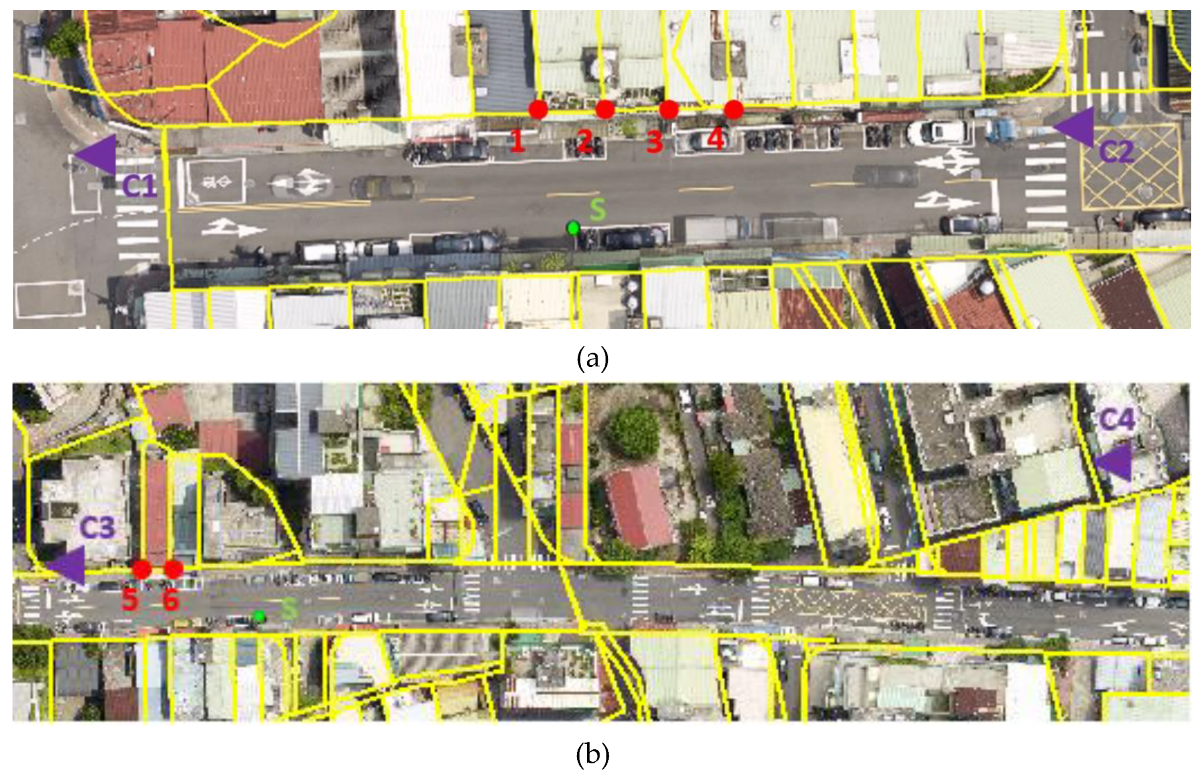
Road corners as supplementary control points, staked out by the free station method
(C1 and C2: control points, S: free station)
LineSurveyed horizontal distance (m)Computed horizontal distance (m)Difference
(m)
SideSurveyed horizontal distance (m)Computed horizontal distance (m)Difference
(m)
S-114.92114.7860.1351–24.8744.8530.021
S-211.35911.2320.1272–35.0274.9940.033
S-39.0628.9330.1293–44.8494.8360.013
S-49.1899.0660.123
Road corners as supplementary control points, staked out by the radiation method
(C1 and S: control points, S: surveying station)
LineSurveyed horizontal distance (m)Computed horizontal distance (m)Difference
(m)
SideSurveyed horizontal distance (m)Computed horizontal distance (m)Difference
(m)
S-114.89014.7780.1121–24.8484.8530.005
S-211.36011.2230.1372–35.0254.9940.031
S-39.0658.9230.1423–44.8094.7780.031
S-49.1359.0570.078
Building corners as supplementary control points, staked out by the free station method
(C3 and C4: control points, S: surveying station
LineSurveyed horizontal distance(m)Computed horizontal distance (m)Difference
(m)
SideSurveyed horizontal distance (m)Computed horizontal distance (m)Difference (m)
S-521.66921.8080.1415–64.944.8240.116
S-617.21417.3420.128

